The IASI Water Deficit Index to Monitor Vegetation Stress and Early Drying in Summer Heatwaves: An Application to Southern Italy

Abstract

The boreal hemisphere has been experiencing increasing extreme hot and dry conditions over the past few decades, consistent with anthropogenic climate change. The continental extension of this phenomenon calls for tools and techniques capable of monitoring the global to regional scales. In this context, satellite data can satisfy the need for global coverage. The main objective we have addressed in the present paper is the capability of infrared satellite observations to monitor the vegetation stress due to increasing drought and heatwaves in summer. We have designed and implemented a new water deficit index (wdi) that exploits satellite observations in the infrared to retrieve humidity, air temperature, and surface temperature simultaneously. These three parameters are combined to provide the water deficit index. The index has been developed based on the Infrared Atmospheric Sounder Interferometer or IASI, which covers the infrared spectral range 645 to 2760 cm⁻¹ with a sampling of 0.25 cm⁻¹. The index has been used to study the 2017 heatwave, which hit continental Europe from May to October. In particular, we have examined southern Italy, where Mediterranean forests suffer from climate change. We have computed the index’s time series and show that it can be used to indicate the atmospheric background conditions associated with meteorological drought. We have also found a good agreement with soil moisture, which suggests that the persistence of an anomalously high water deficit index was an essential driver of the rapid development and evolution of the exceptionally severe 2017 droughts.

1. Introduction

The ECMWF (European Centre for Medium-Range Weather Forecasts) has determined that the winter of 2020 was the hottest winter season ever recorded in Europe (e.g., see https://climate.copernicus.eu/boreal-winter-season-1920-was-far-warmest-winter-season-ever-recorded-europe-0 (accessed on 15 August 2022)). This is an event that is now repeated year after year [1,2], as evidenced by the Copernicus Climate Change Service (C3S) dataset (e.g., see https://climate.copernicus.eu/esotc/2021/globe-in-2021 (accessed on 15 August 2022)), which shows that the last seven years have been the warmest on record, with 2021 varying from the fifth to the seventh warmest.

The present analysis is most relevant to temperate regions and the Mediterranean vegetation. In this respect, ref. [3] discussed the risks of climate change altering sustainable development in the Mediterranean area. Furthermore, in [4], it has been shown that long-lasting droughts induce dieback phenomena in temperate and Mediterranean climate regions, an issue that has also been addressed in [5], which analysed the effect of the 2017 summer heatwave in Europe.

The continental extension of the phenomenon calls for tools and techniques capable of monitoring the global to regional scales. For this reason, we have set up a methodology based on satellite data with the objective of using infrared satellite observations to monitor early drying in summer because of drought and heatwaves.

Vegetation stress due to water deficit is widespread in many countries due to climate change (e.g., see [4,5]). Drought is an extreme natural event typical of semi-arid areas and much of the Mediterranean, especially regions located at middle latitudes. The lack of rain for long periods increases the danger and risk of forest fires in lands rich in vegetation and wooded areas [6]. Furthermore, the lack of rain in semi-arid regions causes water stress (e.g., [7,8]). Therefore, the deficit of rainfall and/or water, in general, requires specific actions to monitor and detect drought conditions aiming to mitigate its adverse impacts on human health, wildlife, and plant communities.

Water deficit can be estimated using (1) meteorological data (e.g., [9,10,11]); and (2) remote sensing (e.g., [12,13,14,15]).

The present study aims at a synergetic use of these two different methods to develop new vegetation dryness indices based on the surface temperature, complemented with atmospheric temperature and the water vapor mixing ratio or parameters depending on it, such as dew point temperature.

In general, the problem has been studied through the use of indexes such as the vegetation dryness index (or VDI), the temperature vegetation dryness index (TVDI), and the improved TVDI (or iTVDI) (among many others, see [16,17,18]). These indices are based on the NDVI (normalized differential vegetation index), the surface temperature, T_s, and the air temperature close to the surface, or T_a. The problem with NDVI is that it is a greenness index and cannot distinguish bare soil from senescent vegetation (e.g., see [19]). In addition, neither T_s nor T_a are directly linked with soil moisture. It should be observed that the use of T_s-NDVI relationships has been long investigated for application to drought assessment, and it has been found to produce inconsistent results in some specific situations (e.g., [20]).

Conversely, we propose to follow the strategy of using surface temperature (T_s), and the dew point temperature (T_d), which are more closely related to surface type and coverage, and soil moisture. The water deficit index is then defined according to the linear difference T_s − T_d.

The water deficit index is meant for analysis at the regional scale; therefore, we need the use of satellite data to ensure the correct spatial coverage and time sampling. Toward this objective, we have used the hyper-spectral satellite infrared sounder (Infrared Atmospheric Sounder Interfemoter or IASI, e.g., [21]) flying on board the European Meteorological Platforms (MetOp). By adequately exploiting IASI observations, we can simultaneously retrieve T_s and T_d, which limit problems of time-space colocation. However, satellite data are available at uneven grid points, making it challenging to check spatial patterns. In this respect, our objective is two-fold: first, we want to define and compute a suitable water deficit index based on direct satellite soundings; and second, we want to define a strategy to resample the sparse satellite retrievals on a regular grid for the better understanding of spatial patterns.

We acknowledge that water deficit indices are common in-field analyses related to horticulture, e.g., irrigation management, evaluation of crop water stress, and so on (e.g., see [6] and references therein). However, in these cases, we are generally in the presence of temporary water deficit anomalies. In contrast, our approach is meant to account for the background atmospheric humidity and temperature related to drought onset and development (e.g., see [22]). For satellite-based analysis, a similar approach has been proposed in [23], using the concept of vapour pressure deficit (VPD), the difference between the saturation and actual vapour pressure for a given time. In contrast, our approach uses T_d, which is related to VPD, and T_s to build the difference T_s − T_d, allowing us to better separate the hot-dry from humid-warm weather conditions.

The paper is organized as follows. Section 2 deals with data and methods; in particular, the section illustrates the IASI retrieval system we have developed and used for the present analysis. Results are shown in Section 3 and discussed in Section 4. Finally, conclusions are drawn in Section 5.

2. Materials and Methods

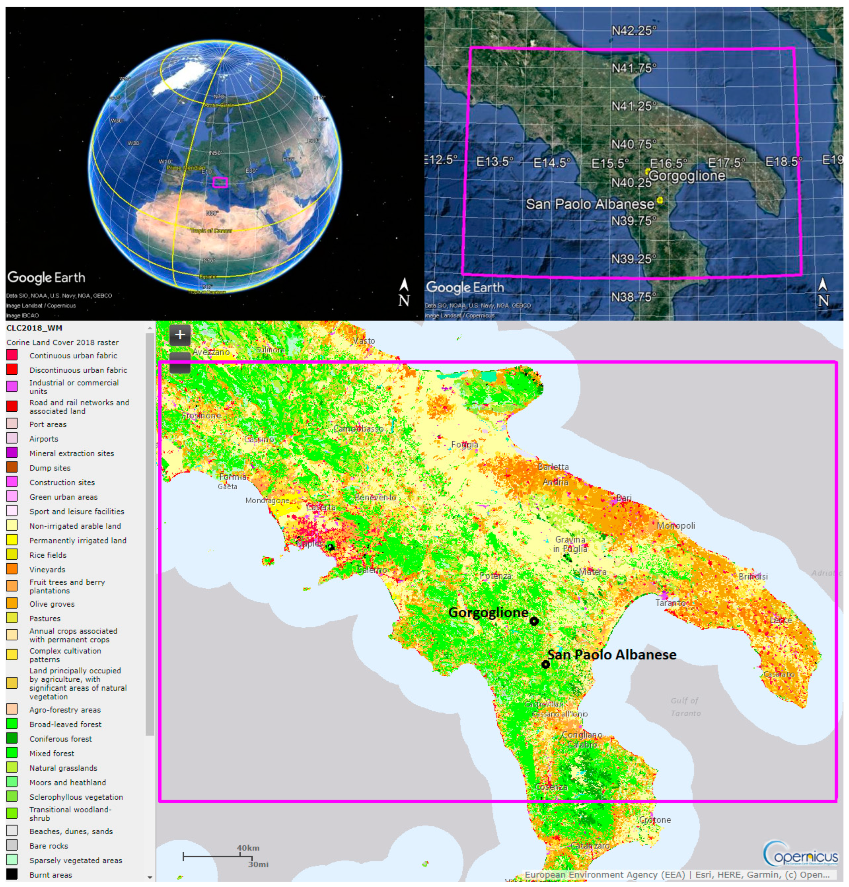
2.1. Material and Data

The retrieval from space observations of T_s and T_d have been performed using the Infrared Atmospheric Sounder Interferometer (or IASI) [21]. IASI has been developed in France by CNES and is flying on board the Metop platforms, which are satellites of the EUMETSAT European Polar System (EPS). IASI has been primarily designed as a meteorological mission; hence, its main objective is to provide relevant information on temperature and water vapour profiles. The spectral coverage of the instrument extends from 645 to 2760 cm⁻¹, and its sampling interval is Δσ = 0.25 cm⁻¹; therefore, the instrument provides 8461 channels, i.e., spectral observations for every spectrum.

IASI is a cross-track scanner with 30 adjacent fields of regard (FOR) per scan, spanning an angular range of ±48.33° on either side of the nadir. The FOR viewing geometry consists of a 2 × 2 matrix of instantaneous fields of views (IFOVs). In turn, the single IFOV has a diameter of 0.8394°, corresponding to a ground resolution of 12 km per nadir for a satellite altitude of 819 km. The 2 × 2 IFOV matrix is centered on the viewing direction. At nadir, a FOR of 4 IASI IFOVs (or pixels) covers the ground a square area of ≈50 × 50 km². The corresponding FORs (among the 30 views) are ±1.67° on each side from the nadir direction. Further details about IASI and its mission objectives are referred to in [21].

Figure 1 shows the target area we have focused on in the paper. The site corresponds to southern Italy, with the Apennine chains covered by forest, as exemplified by the 2018 CORINE land cover (https://land.copernicus.eu/pan-european/corine-land-cover (accessed on 15 August 2022)). The black dots identify two dieback forest areas, where forest monitoring, by ecophysiological and dendrochronological approaches, has been running since 2013 [24].

The two locations circled in the maps of Figure 1 correspond to the forest stands of San Paolo Albanese (40.02° N, 16.34° E, 950–1050 m.a.s.l.) and Gorgoglione (40.40° N, 16.14° E, 800–850 m.a.s.l.), which are suffering from long-lasting drought-induced tree mortality (e.g., [4]). In the San Paolo Albanese site, the vegetation is formed by a pure high forest of Quercus frainetto Ten. for a stand density of 348 trees ha⁻¹. As far as the most affected stands are concerned, recent studies observed that more than 50% of the mature specimens showed symptoms of death, while about 15% died recently [25]. On the other hand, the Gorgoglione woodland is a highly mixed forest, with an average density of about 600 stems ha⁻¹. The vegetation is dominated by Quercus cerris L. (71%), followed by Quercus pubescens L. (25%) and, at a lower density (4%), other species of deciduous trees [25].

The two main studied tree species (i.e., Quercus cerris L. and Quercus pubescens L.) have shown recent drought-induced decline symptoms since the early 2000s (shoot dieback, summer leaf loss, withering, growth decline, and high mortality). According to local reports about the study area, the yearly oak mortality affected ca. 450 ha. The incidence of the decline syndrome raised mortality from 5 to 10%, from 2002 to 2004 [24].

IASI soundings have been acquired for the whole year of 2017 when an intense heat wave hit Europe and the Mediterranean area in summer (e.g., see [5]). For comparison, we have also acquired IASI data for 2020 and 2021.

For a proper comparison with our IASI T_s − T_d index, for the same target area and the year 2017, the Copernicus Global Land Service (https://land.copernicus.eu/global/products (accessed on 15 August 2022)) was used to obtain data about the surface soil moisture ($ssm$) and the leaf area index ($LAI$).

The surface soil moisture was derived by observing the band C SAR onboard the satellite Sentinel-1. Data were provided with a timeliness of one day at a spatial resolution of ~1 km. For details about the $ssm$ product, we refer the interested reader to [26].

The leaf area index was globally estimated at a spatial resolution of about 300 m through a neural net approach. The input to the net was obtained from instantaneous top-of-canopy reflectances from the OLCI (Ocean and Land Colour Imager) instrument onboard the Sentinel-3 satellite, or daily top-of-aerosol reflectances from the PROBA-V satellite. We refer the interested reader to [27] for further details about the LAI data.

Finally, data about the ecophysiological responses of trees for the forest stands of San Paolo Albanese and Gorgoglione were measured and used in the present analysis during two field campaigns performed from July–September in 2020 and 2021.

2.2. Methods

IASI will add unique capabilities to the present study because we were able to simultaneously retrieve $T_s$ and $T_d$ (e.g., [28,29,30,31,32]) from this instrument. To this end, we developed two retrieval prototypes: one for simultaneous inversion of infrared observations (level 2 or L2 prototype), and the second for remapping L2 products on a regular grid (L3 prototype).

The layout of the overall scheme we developed is sketched in Figure 2. The procedure consists of three main steps identified in Figure 2 with grey boxes.

The IASI Level 2 and 3 prototypes have been developed in previous studies. The most up-to-date versions of both schemes can be found in [30,33] for the L2 package and [34] for Level 3 Optimal Interpolation. The digital object identifier (doi) shown in Figure 2 allows the interested reader to open online references where the two schemes are analytically presented. For this reason, they are just summarized in the present paper. In contrast, the Pre-OI scheme is described in more detail, as it implements the equations and formulas needed for calculating the state vector and associated covariance matrix, which are passed to the OI scheme to compute the maps of the water deficit index.

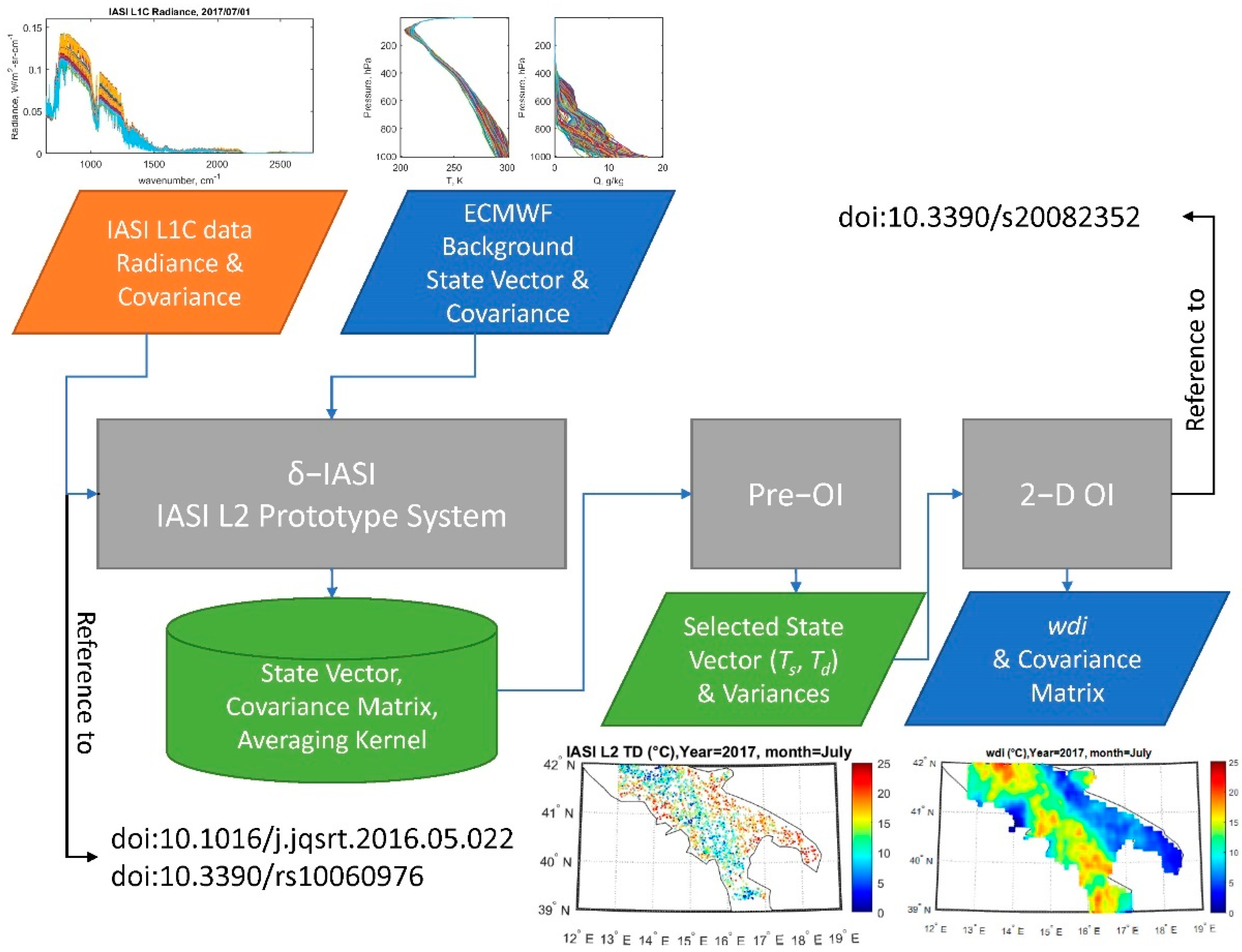
2.2.1. The L2 Retrieval System

The L2 prototype, which we also call δ-IASI, consists of an optimal estimation scheme (e.g., [35]), which simultaneously inverts the full IASI spectrum to retrieve the state vector, which is made up of the surface emissivity ($\epsilon$), the surface temperature ($T_s$), the atmospheric profiles of temperature ($T$), water vapour ($Q$), ozone ($O$), HDO ($D$), carbonyl sulfide or OCS, and scalar scaling factors for the column amount of CO₂, CO, N₂O, CH₄, SO₂, HNO₃, NH₃, and CF₄. However, the parameters relevant to the present analysis are $T_s$, and the atmospheric profiles for $T$ and $Q$. Our L2 prototype for IASI has been variously validated as far as the surface parameters and $T$ and $Q$ profiles are concerned. Validation for surface parameters can be found, e.g., in [32,33], whereas for $T$ and $Q$ they can be found in [30,36].

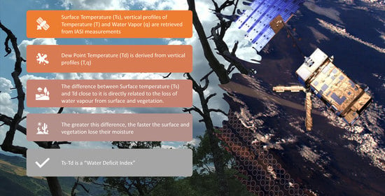
2.2.2. The L2 Pre-OI and the Definition of the Water Deficit Index

Regarding Figure 2, the Pre-OI acts on the IASI Level 2 data to extract the geophysical parameters close to the surface and compute the water deficit index and its variance to input the final optimal interpolation scheme. From the profiles of $T$ and $Q$, we considered only the elements, which correspond to the lowermost atmospheric layer, say $T_1$ (in units of K) and $Q_1$ (in units of gr/Kg). The corresponding layer pressure was denoted with $P_1$ (in units of hPa). From the L2 products, we also extracted the surface temperature, $T_s$. The three parameters ($T_s, T_1,Q_1)$ were piled up in a vector, ${\mathit{x}}_1$ of size $n=3$, whose covariance matrix was denoted with ${\mathit{S}}_1,$ whose size was $n\times n.$ Both ${\mathit{x}}_1$, ${\mathit{S}}_1$ are outputs of the IASI L2 system.

The computation of the dew point temperature, $T_d$, involves the calculation of the actual and saturation water vapour pressures. These are referred to as $P_w$and $P_{ws}$, respectively. From $Q_1$, we can compute $P_w$ according to:

$$P_w={10}^{-3}{P}_1{Q}_1\frac{R_w}{R_{air}}=\beta P_1{Q}_1;\beta ={10}^{-3}\frac{R_w}{R_{air}}$$

(1)

with $P_w$ in hPa and where $R_w=461.5$ J K⁻¹ Kg⁻¹ and $R_{air}=286.9$ J K⁻¹Kg⁻¹ are the specific gas constants of water vapour and air, respectively. According to [37], $P_{ws}$ is computed with the formula:

$$P_{ws}={10}^{-2}\frac{\exp \left(a_1-\frac{a_2}{t_1+a_3}\right)}{{\left(t_1+a_4\right)}^{a_5}}$$

(2)

with $t_1=T_1-273.15$ (temperature in degrees Celsius) and $P_{ws}$ in hPa. Equation (2) is valid for $t_1>0$ (vapor pressure of water), and where $a_1=34.494, a_2=4924.99, a_3=237.1, a_4=105, a_5=1.57$ are fit parameters that in case $t_1$ are expressed in degrees Celsius. From (1) and (2), we obtain the fractional relative humidity:

$$rh=\frac{P_w}{P_{ws}}$$

(3)

From (1) and (2), we can also compute the vapour pressure deficit or $VPD=P_{ws}-P_w$. Finally, the dew point temperature, $T_d$ can be calculated by using the well-known Magnus formula (e.g., [38]):

$$t_d=\frac{cx}{b-x}, x=\ln \left(rh\right)+\frac{b{t}_1}{c+t_1}$$

(4)

where $t_d$ is in degrees Celsius (we will use $T_d$ when referring to degrees Kelvin units), and $b=17.62$ (dimensionless), $c=243.12$ C. Finally, the IASI-based water deficit index, $wdi$, is defined according to:

$$wdi=T_s-T_d=t_s-t_d$$

(5)

Equation (5) stresses that the index can be computed indifferently with both temperatures in K or C degrees, although the computation of the dew point temperature has to be performed in C, according to Equation (4), before converting it to K.

For the application of the optimal interpolation to the mapping of the water deficit index, we also need the variance of the index, ${\sigma }_{wdi}^2$. Considering the chain of equations from (2) to (5), we can formally write $wdi$ as a function $wdi=f\left(T_s, T_1,Q_1\right)$, from which, using the usual rule of variance propagation (see, e.g., [39]), we obtain:

$${\sigma }_{wdi}^2={\mathit{g}}^{\mathit{t}}{\mathit{S}}_1\mathit{g}$$

(6)

with the superscript t indicating the transpose operation, and

$$\mathit{g}={\left(\frac{\partial f}{\partial T_s},\frac{\partial f}{\partial T_1},\frac{\partial f}{\partial Q_1}\right)}^t$$

(7)

We stress that the parameters defined by Equations (5) and (6) have to be computed for the IASI retrievals and the ECMWF background, as shown in the diagram of Figure 2. For the background, the covariance matrix is assumed to be diagonal, as we use background derived from climatology (see [29]) for which we do not consider correlation among air temperature, humidity, and surface temperature.

Considering that

$$f\left(T_s, T_1,Q_1\right)=T_s-T_d=t_s-t_d=t_s-\frac{cx}{b-x}$$

(8)

we have

$$\begin{array}{cc}\frac{\partial f}{\partial T_s}=\frac{\partial f}{\partial t_s}=1& \\ \frac{\partial f}{\partial T_1}=\frac{\partial f}{\partial t_1}=\frac{\partial f}{\partial x}\frac{\partial x}{\partial t_1}=-\frac{cb}{{\left(b-x\right)}^2}\left(-\frac{a_2}{{\left(t_1+a_3\right)}^2}+\frac{a_5}{\left(t_1+a_4\right)}+\frac{bc}{{\left(t_1+c\right)}^2}\right)& \\ \frac{\partial f}{\partial Q_1}=\frac{\partial f}{\partial x}\frac{\partial x}{\partial Q_1}=-\frac{cb}{{\left(b-x\right)}^2}\frac{1}{Q_1}& \end{array}$$

(9)

The parameter $wdi,$ when referring to a surface covered by vegetation or crops, can help to understand the water stress or deficit during long-lasting droughts or heatwaves. This is because vegetation releases water into the atmosphere through transpiration. The process involves the vaporization of liquid water in plant tissues and the consequent release of vapour into the atmosphere (for example, see [40])). Similar to direct evaporation, transpiration depends on the amount of energy available: solar radiation, wind, and vapour pressure gradient at the surface–atmosphere interface. Consequently, solar radiation, air temperature and humidity, and wind velocity must be considered when evaluating and assessing a satellite-based index to quantify water deficit.

In Equation (5), the role of energy supply is modelled with $T_s$. The sun’s radiation will cause a rapid increase in the surface temperature of the land. On the other hand, $T_d$ will take into account both air temperature and air humidity. The effect of wind is more difficult to introduce. However, drought and heatwave conditions minimize the spatial gradient and wind intensity. The air subsidence and low intense pressure gradients characterize meteorological conditions that favour summer heatwaves.

It is also important to stress that evaporation and transpiration co-occur, and it is not easy to distinguish between the two processes. For this reason, we mention evapotranspiration when referring to the water exchange between vegetation and the air. In addition to water availability in the topsoil, evaporation from the cultivated terrain depends, as already mentioned, on the amount of impinging solar radiation. The solar energy at the surface decreases during crop growth because its foliage or canopy shadows the area below from the sun’s rays as the crop develops. Therefore, water is predominately lost by soil evaporation when the crop is small, or when the leaves are not well developed. However, transpiration becomes the main process once the crop and leaves are well developed and completely cover the soil.

With this in mind, the parameter $wdi$ can help to identify different regimes of water deficit:

1.

$wdi\gg 0;$this regime characterizes very hot and dry conditions that favour evapotranspiration. Furthermore, in this regime, the evapotranspiration increases almost linearly with the wind speed (e.g., [40]);

2.

$wdi\ge 0$; this regime characterizes warm and humid conditions when the air is already close to saturation; therefore, less additional water can be stored, so the evapotranspiration rate is even lower than for arid land;

3.

$wdi\le 0;$this is the regime $T_s<T_d$, and therefore the vapour condenses in liquid water at the surface.

2.2.3. The 2-D OI scheme

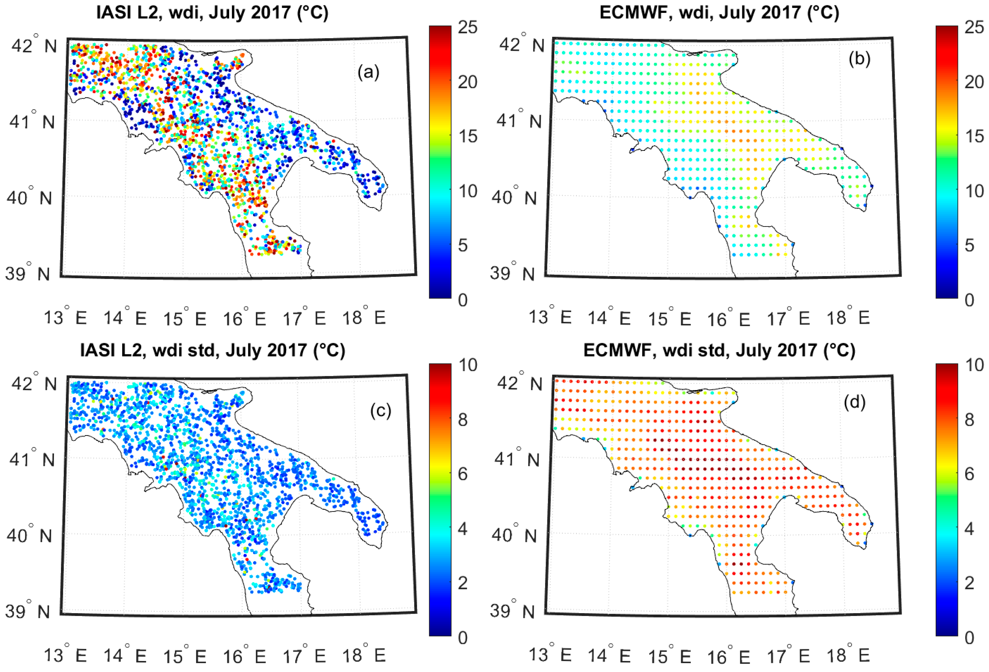
It is worth noting that when $wdi$ is determined by L2 satellite observations, as in our case, we obtain data that are sparse and not homogeneously covering a given spatial region. Therefore, to better compare with other data sources and perform a correct collocation with stations at the ground, we used a resampling tool, which can remap $wdi$ data to a regular grid. To this end, we used the tool developed in [34]. The technique is based on a 2-dimensional (2D) optimal interpolation (OI) scheme, and is derived from the broad class of Kalman filter or Bayesian estimation theory. For further details, we refer the interested reader to [34].

The steps involved in the mapping on a regular grid are exemplified in Figure 3 using the IASI retrieval for $wdi$ for July 2017. Figure 3a,c show the IASI data points for $wdi$, and its square root of the variance (standard deviation) as estimated by the L2 retrieval scheme and the Pre-OI step (see Figure 2). These values are accumulated considering all the IASI overpasses for July 2017. As said before, the IASI scan pattern is made up of footprints with circular diameters of about 12 km at nadir, and the scanning lines are 50 km apart along the flight direction of the satellite. The IASI scan pattern over the target area for a single overpass is shown in Figure 4 for the benefit of the reader. Comparing Figure 3 with Figure 3a,c, it can be seen that after one month, the IASI clear sky footprints (we stress that we use only observations in a clear sky, which is diagnosed based on a stand-alone algorithm for cloud detection, e.g., [41]) are densely distributed over the area much more than the single IASI scan pattern overpass. The monthly ensemble of satellite overpasses improves the sampling of spatial data, and therefore allows, for example, a better comparison with in situ observations. We use the ensemble of multiple observations to build a map with a better spatial sampling. Towards this objective, we use the 2-D OI method, which remaps the data into a grid with a finer mesh than the original data.

The final mesh we use has a spatial sampling of 0.05° × 0.05°. Another important aspect of OI remapping is the use of background fields. These fields are built up by using the time and space co-located ECMWF (European Centre for Medium-Range Weather Forecasts) analysis. The ECMWF fields are available on a grid-mesh of 0.125° × 0.125°, and, for the case at hand, the values for $wdi$ and its square root of the variance, i.e., standard deviation, are exemplified in Figure 3b,d, respectively. Based on the coarse ECMWF background, the un-gridded L2 IASI observations and the 2-D OI yields the results are shown in Figure 5; that is, the maps of $wdi$ (panel (a)) and its standard deviation (panel (b)) at a sampling of 0.05° × 0.05°. In this process, we lose temporal resolution, but we obtain a map with improved spatial sampling and precision, as shown by the standard deviation map, which, apart from boundary effects, is one °C or less.

3. Results

The rise and fall of the exceptionally hot and dry summer are well captured by the monthly time series of $wdi$ maps shown in Figure 6. Of particular interest for us is the Apennine chain, which is covered by broad-leaved, deciduous forests. If we compare Figure 5 to the land cover map shown in Figure 1, we see that the $wdi$ closely follows the forested area in the summer season. In July and August 2017, the index was above ~10 °C in the regions covered by forests, which shows that the vegetation ecosystem was suffering from a water deficit.

To understand the index’s sensitivity to heat waves, we have compared the $wdi$ parameter over three consecutive years, 2017, 2020, and 2021, for July. We know that July 2020 has been relatively wetter than 2017 and 2021 (e.g., see https://climate.copernicus.eu/esotc/2021 (accessed on 15 August 2022)). The comparison is shown in Figure 7, and we see that $wdi$ is able to indicate that the year 2020 was less warm than the other two. This situation is reflected in the soil moisture maps shown for the same target area and year and month. When we focus on the forested area, especially in the southern part of the map, we see that the soil moisture follows the same spatial-time evolution as $wdi$ and, in particular, the soil moisture is lower in 2017 and 2021 than in 2020. This is a significant result because it shows that the $wdi$ is capable of capturing processes at the surface–atmosphere interface. A large $wdi$ means a high rate of evapotranspiration; that is, trees lose water in the atmosphere. The fact that the soil moisture is getting lower means that the vegetation can catch less water from the surface.

The anti-correlation between $wdi$ and soil moisture proves that $wdi$ is a good metric for monitoring water deficit during intense heatwaves. The more significant values we saw in summer are not merely a consequence of the hotter weather, but also reflects the decrease in water vapour exchange between the surface and the atmosphere. We stress that, unlike other indices, $wdi$ considers the surface-air temperature and humidity fields simultaneously.

A further comparison with other parameters sensitive to vegetation stress is shown in Figure 8 and Figure 9. Concerning the 2017 heatwave, Figure 8 compares the surface soil moisture ($ssm$) against $wdi$ for the period June to August. It is seen that while $wdi$ tends to increase with time, $ssm$ does the opposite. The leaf area index (LAI) is another crucial parameter to be monitored for investigating vegetation stress. Indeed, under the action of an intense heat wave, trees tend to lose leaves to protect from the fierce evapotranspiration. Trees use this mechanism, e.g., in winter, when the light is not enough to sustain the photosynthesis activity. The comparison with $\mathrm{LAI}$is shown in Figure 9, and we see that consistently with the increasing $wdi$ behaviour, $\mathrm{LAI}$ is decreasing from June to July. In normal situations, the $\mathrm{LAI}$. decrease is not expected in the summer when there is a more significant availability of light to sustain photosynthesis.

We have checked that the good consistency among $ssm$, $\mathrm{LAI},$ and $wdi$ also persists at the local scale. In fact, for the two stations of S. Paolo Albanese and Gorgoglione, shown in Figure 1, we have computed the monthly time series of $ssm$ and $wdi$ for 2017. The time series are shown in Figure 10, and we see that starting from May until September, $wdi$ goes up, whereas $ssm$ has the opposite behaviour. Again, this is an important result because it shows that the $wdi$ is capturing a water deficit condition for the vegetation, especially in the area where we know there are declining trees [6,24].

The most striking agreement is seen when comparing in situ observations for the flux exchange of CO₂ and H₂O from trees to the $wdi$ parameter. In the summers of 2020 and 2021, CO₂ exchange measurements were performed at the leaf scale on declining and non-declining Q. frainetto trees growing at the S. Paolo Albanese study site. In each tree, net photosynthesis rate (An, µmolCO₂ m⁻² s⁻¹), stomatal conductance (gsw, mmolH₂O m⁻² s⁻¹), and intrinsic water use efficiency (WUEi, µmolCO₂ mmol⁻¹ H₂O) were measured by using a portable Photosynthesis System LiCOR 6400xt equipped with a 6400-40 Leaf Chamber Fluorometer.

In the summers of 2020 and 2021, the ecophysiological response of Q. frainetto trees exhibiting decline and non-decline symptoms is shown in Figure 11. In 2020, when no heatwave occurred, Q. frainetto ecophysiological responses were similar for declining and non-declining trees, suggesting that there was no evident sign of water stress in the summer of 2020. From Figure 7, we see that $wdi$is in fact below 10 °C in July. In contrast, in 2021, not only is the water vapour exchange more than doubled, showing that the evapotranspiration has increased because of the larger difference $T_s-T_d$, but also the declining trees behave differently with respect to the non-declining vegetation, showing that the non-declining trees are suffering from the water deficit much more than the healthy vegetation.

It is also interesting to note that CO_2, flux exchange exhibited the opposite behaviour to H₂O. In the summer of 2020, when there were good climatic conditions, we observed an exchange larger than in 2021. In 2021, the results showed that the vegetation had reduced photosynthesis activity because of stress conditions.

4. Discussion

In the summer of 2017, southern Europe and the Euro-Mediterranean were hit by an exceptional heat wave [6,42]. After an outstandingly warm June in western Europe, the heat returned to southern Italy in July. It contributed to more than 400 wildfires, which destroyed approximately 800 km² of forest and vegetated areas. The number of fires has been unprecedented in the last 20 years. Furthermore, early August saw a particularly intense heat wave described as the “worst heat wave since 2003”, with the air temperature above 40 °C in many parts of Italy [42].

In the quest for possible satellite indices to assess and possibly mitigate the effect of long-lasting drought on vegetation, we have devised an index, $wdi,$ which takes advantage of the IASI capability to retrieve surface data simultaneously with atmospheric parameters. Other methods that use satellite data exploit the visible region of the electromagnetic spectrum (e.g., NDVI, NDMI, and related indices) or the microwave band (e.g., $ssm$ and LAI). The normalized difference moisture index (NDMI) (e.g., [43]) is mainly intended to detect humidity in vegetation using a combination of near-infrared (NIR) and short-wave infrared (SWIR) spectral bands. The index NDMI and the original greenness index, NDVI, with the same $ssm$, have also been used coupled to surface temperature and air temperature (e.g., see [8,11,12,13,14,18]). Other tools have tried to couple surface temperature and the humidity field, e.g., [6].

In contrast, our $wdi$ exploits the thermal band of the Earth’s emission spectrum and simultaneously uses the surface temperature, air temperature, and humidity. To our knowledge, this combination is unique. In effect, the water deficit index we have defined can monitor water deficit and assess vegetation stress, as the comparison with in situ measurements has demonstrated. It can be used complementary to $ssm$, LAI, and the set of NDVI-related indices to better understand the intensity and danger of heatwaves for the vegetation. Sequences of increasing $wdi$ can help to identify the onset of water deficit for the vegetation, hence the increased risk of fire, especially in forests.

The $wdi$ index is meant to identify regions where particular weather conditions can produce water deficits. The index is not intended as an estimate or an estimator of evapotranspiration. This process is also affected by vegetation/crop characteristics, environmental conditions, and cultivation types. Therefore, there is too much variability, which cannot be condensed into a single index. The $wdi$ parameter is a bulk index, which can help to monitor forest and wood regions suffering from long-lasting droughts because of adverse weather conditions. It can be mapped on a regional and even global scale, allowing us to monitor drought processes at a glance. The $wdi$ maps could be important to monitor and evaluate the risk of fires in the large forested area, which is otherwise inaccessible. In addition, we have shown that in regions where the vegetal ecosystem has a particular fragility to water deficit, the index can soon quantify the possible danger and require more accurate in situ observations.

In this respect, $wdi$ is most effective in the case of a heatwave. In the wintertime, for example, large values of $wdi$ could be linked to a dry atmosphere and low air temperature. In effect, this is the case in January 2017 for the more southern area on the map of Figure 5, which belongs to the high mountains of the Sila chain. Additionally, in summer, very humid and warm conditions could lead to $wdi~0$. For example, this is the case for the coastal regions in July–August 2017, as seen again in the map in Figure 5. For these cases, it is better to look separately at the maps of $T_s$and $T_d$. In this respect, we observe that the dew point temperature has been individuated as a key parameter to compute sophisticated indicators of health stress for human beings during heatwaves [44].

Some words of caution should also be said about the temporal sampling of $wd$i. The occasional occurrence of a high $wdi$ for one day should be of no concern. Drought is a process that takes several days or months. The severity of the process depends on its time continuity and persistence. Therefore, it is crucial to assess the persistence of the process, which can be done by looking at the time series. Averaging over several days can help to understand the persistence of the phenomenon. Another important point concerns the capability of the retrieval system to solve the daily cycle, which cannot be done with the present polar satellite IASI instrument. During the night, the surface temperature could go below the dew point temperature and cause water vapour to condense at the surface. Therefore, it could be interesting to examine day and night separately. Hopefully, this could be the case when the MTG-IRS (https://www.eumetsat.int/mtg-infrared-sounder (accessed on 15 August 2022)) is put in orbit.

5. Conclusions

Exploiting the capability of the IASI instrument to perform simultaneous retrievals of surface and thermodynamical parameters, we have developed an index called the water deficit index, or $wdi$. The index is intended to be used in the case of evident droughts, as it can assess the severe water deficit of vegetation, and in particular, forests.

The tool has been exemplified in a target area in the south of Italy, which suffered from an intense drought and heatwave in 2017. When the heatwave is developing, we have shown, with the help of correlative observations of surface soil moisture and the leaf area index, that $wdi$ can assess the severity of the water deficit. Of particular interest is the anti-correlation with the surface soil moisture. The soil water content and the ability of the soil to transport water to the roots govern the transpiration rate of vegetation. In cases where the $wdi$ becomes large, we have found that $ssm$gets smaller, which shows how $wdi$ is capable of capturing processes occurring at the surface–atmosphere interface.

The possible usage of $wdi$ includes monitoring large forested areas for the increased risks of wildfire and assessing mitigation measures for regions whose green ecosystems are more fragile and in danger because of climate change.

References

1. Voosen, P. Global Temperatures in 2020 Tied Record Highs. Science 2021, 371, 334–335. [Google Scholar] [CrossRef] [PubMed]
2. Cheng, L.; Abraham, J.; Trenberth, K.E.; Fasullo, J.; Boyer, T.; Mann, M.E.; Zhu, J.; Wang, F.; Locarnini, R.; Li, Y.; et al. Another Record: Ocean Warming Continues through 2021 despite La Niña Conditions. Adv. Atmos. Sci. 2022, 39, 373–385. [Google Scholar] [CrossRef] [PubMed]
3. Cramer, W.; Guiot, J.; Fader, M.; Garrabou, J.; Gattuso, J.-P.; Iglesias, A.; Lange, M.A.; Lionello, P.; Llasat, M.C.; Paz, S.; et al. Climate Change and Interconnected Risks to Sustainable Development in the Mediterranean. Nat. Clim. Chang. 2018, 8, 972–980. [Google Scholar] [CrossRef]
4. Rita, A.; Camarero, J.J.; Nolè, A.; Borghetti, M.; Brunetti, M.; Pergola, N.; Serio, C.; Vicente-Serrano, S.M.; Tramutoli, V.; Ripullone, F. The Impact of Drought Spells on Forests Depends on Site Conditions: The Case of 2017 Summer Heat Wave in Southern Europe. Glob. Chang. Biol. 2020, 26, 851–863. [Google Scholar] [CrossRef]
5. Anderegg, W.R.L.; Trugman, A.T.; Badgley, G.; Anderson, C.M.; Bartuska, A.; Ciais, P.; Cullenward, D.; Field, C.B.; Freeman, J.; Goetz, S.J.; et al. Climate-Driven Risks to the Climate Mitigation Potential of Forests. Science 2020, 368, eaaz7005. [Google Scholar] [CrossRef]
6. Mishra, A.K.; Singh, V.P. A Review of Drought Concepts. J. Hydrol. 2010, 391, 202–216. [Google Scholar] [CrossRef]
7. Feiziasl, V.; Jafarzadeh, J.; Sadeghzadeh, B.; Mousavi Shalmani, M.A. Water Deficit Index to Evaluate Water Stress Status and Drought Tolerance of Rainfed Barley Genotypes in Cold Semi-Arid Area of Iran. Agric. Water Manag. 2022, 262, 107395. [Google Scholar] [CrossRef]
8. Spinoni, J.; Barbosa, P.; De Jager, A.; McCormick, N.; Naumann, G.; Vogt, J.V.; Magni, D.; Masante, D.; Mazzeschi, M. A New Global Database of Meteorological Drought Events from 1951 to 2016. J. Hydrol. Reg. Stud. 2019, 22, 100593. [Google Scholar] [CrossRef]
9. Sutanto, S.J.; van der Weert, M.; Wanders, N.; Blauhut, V.; Van Lanen, H.A.J. Moving from Drought Hazard to Impact Forecasts. Nat. Commun. 2019, 10, 4945. [Google Scholar] [CrossRef]
10. Stoyanova, J.S.; Georgiev, C.G. SVAT Modelling in Support to Flood Risk Assessment in Bulgaria. Atmos. Res. 2013, 123, 384–399. [Google Scholar] [CrossRef]
11. Gouveia, C.; Trigo, R.M.; DaCamara, C.C. Drought and Vegetation Stress Monitoring in Portugal Using Satellite Data. Nat. Hazards Earth Syst. Sci. 2009, 9, 185–195. [Google Scholar] [CrossRef]
12. Bento, V.; Trigo, I.; Gouveia, C.; DaCamara, C. Contribution of Land Surface Temperature (TCI) to Vegetation Health Index: A Comparative Study Using Clear Sky and All-Weather Climate Data Records. Remote Sens. 2018, 10, 1324. [Google Scholar] [CrossRef]
13. Stoyanova, J.; Georgiev, C.; Neytchev, P.; Kulishev, A. Spatial-Temporal Variability of Land Surface Dry Anomalies in Climatic Aspect: Biogeophysical Insight by Meteosat Observations and SVAT Modeling. Atmosphere 2019, 10, 636. [Google Scholar] [CrossRef]
14. Feldman, A.F.; Short Gianotti, D.J.; Trigo, I.F.; Salvucci, G.D.; Entekhabi, D. Land-Atmosphere Drivers of Landscape-Scale Plant Water Content Loss. Geophys. Res. Lett. 2020, 47, e2020GL090331. [Google Scholar] [CrossRef]
15. Vicente-Serrano, S.M.; Pons-Fernández, X.; Cuadrat-Prats, J.M. Mapping Soil Moisture in the Central Ebro River Valley (Northeast Spain) with Landsat and NOAA Satellite Imagery: A Comparison with Meteorological Data. Int. J. Remote Sens. 2004, 25, 4325–4350. [Google Scholar] [CrossRef]
16. Vicente-Serrano, S.M.; Cuadrat-Prats, J.M.; Romo, A. Aridity Influence on Vegetation Patterns in the Middle Ebro Valley (Spain): Evaluation by Means of AVHRR Images and Climate Interpolation Techniques. J. Arid Environ. 2006, 66, 353–375. [Google Scholar] [CrossRef]
17. Chen, S.; Wen, Z.; Jiang, H.; Zhao, Q.; Zhang, X.; Chen, Y. Temperature Vegetation Dryness Index Estimation of Soil Moisture under Different Tree Species. Sustainability 2015, 7, 11401–11417. [Google Scholar] [CrossRef]
18. Masiello, G.; Cersosimo, A.; Mastro, P.; Serio, C.; Venafra, S.; Pasquariello, P. Emissivity-Based Vegetation Indices to Monitor Deforestation and Forest Degradation in the Congo Basin Rainforest. In Proceedings of the Remote Sensing for Agriculture, Ecosystems, and Hydrology XXII, Online, 20 September 2020; Neale, C.M., Maltese, A., Eds.; p. 17. [Google Scholar]
19. Karnieli, A.; Agam, N.; Pinker, R.T.; Anderson, M.; Imhoff, M.L.; Gutman, G.G.; Panov, N.; Goldberg, A. Use of NDVI and Land Surface Temperature for Drought Assessment: Merits and Limitations. J. Clim. 2010, 23, 618–633. [Google Scholar] [CrossRef]
20. Ru, C.; Hu, X.; Wang, W.; Ran, H.; Song, T.; Guo, Y. Evaluation of the Crop Water Stress Index as an Indicator for the Diagnosis of Grapevine Water Deficiency in Greenhouses. Horticulturae 2020, 6, 86. [Google Scholar] [CrossRef]
21. Hilton, F.; Armante, R.; August, T.; Barnet, C.; Bouchard, A.; Camy-Peyret, C.; Capelle, V.; Clarisse, L.; Clerbaux, C.; Coheur, P.-F.; et al. Hyperspectral Earth Observation from IASI: Five Years of Accomplishments. Bull. Am. Meteorol. Soc. 2012, 93, 347–370. [Google Scholar] [CrossRef]
22. Behrangi, A.; Loikith, P.; Fetzer, E.; Nguyen, H.; Granger, S. Utilizing Humidity and Temperature Data to Advance Monitoring and Prediction of Meteorological Drought. Climate 2015, 3, 999–1017. [Google Scholar] [CrossRef]
23. Gentilesca, T.; Camarero, J.; Colangelo, M.; Nolè, A.; Ripullone, F. Drought-Induced Oak Decline in the Western Mediterranean Region: An Overview on Current Evidences, Mechanisms and Management Options to Improve Forest Resilience. iForest 2017, 10, 796–806. [Google Scholar] [CrossRef]
24. Ripullone, F.; Camarero, J.J.; Colangelo, M.; Voltas, J. Variation in the Access to Deep Soil Water Pools Explains Tree-to-Tree Differences in Drought-Triggered Dieback of Mediterranean Oaks. Tree Physiol. 2020, 40, 591–604. [Google Scholar] [CrossRef] [PubMed]
25. Colangelo, M.; Camarero, J.J.; Borghetti, M.; Gentilesca, T.; Oliva, J.; Redondo, M.-A.; Ripullone, F. Drought and Phytophthora Are Associated with the Decline of Oak Species in Southern Italy. Front. Plant Sci. 2018, 9, 1595. [Google Scholar] [CrossRef] [PubMed]
26. Bauer-Marschallinger, B.; Freeman, V.; Cao, S.; Paulik, C.; Schaufler, S.; Stachl, T.; Modanesi, S.; Massari, C.; Ciabatta, L.; Brocca, L.; et al. Toward Global Soil Moisture Monitoring with Sentinel-1: Harnessing Assets and Overcoming Obstacles. IEEE Trans. Geosci. Remote Sens. 2019, 57, 520–539. [Google Scholar] [CrossRef]
27. Fuster, B.; Sánchez-Zapero, J.; Camacho, F.; García-Santos, V.; Verger, A.; Lacaze, R.; Weiss, M.; Baret, F.; Smets, B. Quality Assessment of PROBA-V LAI, FAPAR and FCOVER Collection 300 m Products of Copernicus Global Land Service. Remote Sens. 2020, 12, 1017. [Google Scholar] [CrossRef]
28. Amato, U.; Masiello, G.; Serio, C.; Viggiano, M. The σ-IASI Code for the Calculation of Infrared Atmospheric Radiance and Its Derivatives. Environ. Model. Softw. 2002, 17, 651–667. [Google Scholar] [CrossRef]
29. Carissimo, A.; De Feis, I.; Serio, C. The Physical Retrieval Methodology for IASI: The δ-IASI Code. Environ. Model. Softw. 2005, 20, 1111–1126. [Google Scholar] [CrossRef]
30. Liuzzi, G.; Masiello, G.; Serio, C.; Venafra, S.; Camy-Peyret, C. Physical Inversion of the Full IASI Spectra: Assessment of Atmospheric Parameters Retrievals, Consistency of Spectroscopy and Forward Modelling. J. Quant. Spectrosc. Radiat. Transf. 2016, 182, 128–157. [Google Scholar] [CrossRef]
31. Serio, C.; Masiello, G.; Liuzzi, G. Demonstration of Random Projections Applied to the Retrieval Problem of Geophysical Parameters from Hyper-Spectral Infrared Observations. Appl. Opt. 2016, 55, 6576–6587. [Google Scholar] [CrossRef]
32. Masiello, G.; Serio, C.; Venafra, S.; DeFeis, I.; Borbas, E.E. Diurnal Variation in Sahara Desert Sand Emissivity during the Dry Season from IASI Observations: Diurnal Emissivity Variation. J. Geophys. Res. Atmos. 2014, 119, 1626–1638. [Google Scholar] [CrossRef]
33. Masiello, G.; Serio, C.; Venafra, S.; Liuzzi, G.; Poutier, L.; Göttsche, F.-M. Physical Retrieval of Land Surface Emissivity Spectra from Hyper-Spectral Infrared Observations and Validation with In Situ Measurements. Remote Sens. 2018, 10, 976. [Google Scholar] [CrossRef]
34. De Feis, I.; Masiello, G.; Cersosimo, A. Optimal Interpolation for Infrared Products from Hyperspectral Satellite Imagers and Sounders. Sensors 2020, 20, 2352. [Google Scholar] [CrossRef] [PubMed]
35. Rodgers, C.D. Inverse Methods for Atmospheric Sounding: Theory and Practice; Series on Atmospheric, Oceanic and Planetary Physics; World Scientific: Singapore, 2000; ISBN 978-981-02-2740-1. [Google Scholar]
36. Masiello, G.; Serio, C.; Deleporte, T.; Herbin, H.; Di Girolamo, P.; Champollion, C.; Behrendt, A.; Bosser, P.; Bock, O.; Wulfmeyer, V.; et al. Comparison of IASI Water Vapour Products over Complex Terrain with COPS Campaign Data. Meteorol. Z. 2013, 22, 471–487. [Google Scholar] [CrossRef]
37. Huang, J. A Simple Accurate Formula for Calculating Saturation Vapor Pressure of Water and Ice. J. Appl. Meteorol. Climatol. 2018, 57, 1265–1272. [Google Scholar] [CrossRef]
38. Sonntag, D. Important New Values of the Physical Constants of 1986, Vapour Pressure Formulations Based on the ITS-90, and Psychrometer Formulae. Z. Meteorol. 1990, 40, 340–344. [Google Scholar]
39. Tellinghuisen, J. Statistical Error Propagation. J. Phys. Chem. A 2001, 105, 3917–3921. [Google Scholar] [CrossRef]
40. Allen, R.G.; Pereira, L.S.; Raes, D.; Smith, M. Crop Evapotranspiration: Guidelines for Computing Crop Water Requirements; FAO Irrigation and Drainage Paper; Food and Agriculture Organization of the United Nations: Rome, Italy, 1998; ISBN 978-92-5-104219-9. [Google Scholar]
41. Amato, U.; Lavanant, L.; Liuzzi, G.; Masiello, G.; Serio, C.; Stuhlmann, R.; Tjemkes, S.A. Cloud Mask via Cumulative Discriminant Analysis Applied to Satellite Infrared Observations: Scientific Basis and Initial Evaluation. Atmos. Meas. Tech. 2014, 7, 3355–3372. [Google Scholar] [CrossRef]
42. Kew, S.F.; Philip, S.Y.; Jan van Oldenborgh, G.; van der Schrier, G.; Otto, F.E.L.; Vautard, R. The Exceptional Summer Heat Wave in Southern Europe 2017. Bull. Am. Meteorol. Soc. 2019, 100, S49–S53. [Google Scholar] [CrossRef]
43. 4Khanmohammadi, F.; Homaee, M.; Noroozi, A.A. Soil Moisture Estimating with NDVI and Land Surface Temperature and Normalized Moisture Index Using MODIS Images. J. Water Soil Resour. Conserv. 2015, 4, 37–45. [Google Scholar]
44. Lee, S.-Y.; Lung, S.-C.C.; Chiu, P.-G.; Wang, W.-C.; Tsai, I.-C.; Lin, T.-H. Northern Hemisphere Urban Heat Stress and Associated Labor Hour Hazard from ERA5 Reanalysis. IJERPH 2022, 19, 8163. [Google Scholar] [CrossRef] [PubMed]
Figure 1. Target region for which IASI data have been selected for the present analysis. The figure also shows the CORINE land cover for 2018 to help identify forest regions, which are primarily of interest for this study. The two upper panels help to determine the target area (magenta square) on the globe and Italy.
Land 11 01366 g001
Figure 2. Schematic flow chart of the methodology developed in the present study to yield Level 3 monthly maps of the water deficit index [30,33,34].
Land 11 01366 g002
Figure 3. July 2017. IASI L2 products for w d i (panel (a)) and its standard deviation (panel (c)) over the target area. The figure also shows the ECMWF background field (both mean (panel (b) and standard deviation (d)) at its native spatial resolution of 0.125° × 0.125°.
Land 11 01366 g003
Figure 4. Target region showing the IASI footprint scan pattern (red ovals) for one single overpass. The IASI morning overpass for May, the first of 2020 is shown in the figure.
Land 11 01366 g004
Figure 5. Level 3 map at a grid step of 0.05° for the index w d i obtained from the source data shown in Figure 3 (panel (a)) and its standard deviation (panel (b)). The map is exemplified for July 2017.
Land 11 01366 g005
Figure 6. Level 3 map at a grid step of 0.05 degrees for the index w d i for 2017.
Land 11 01366 g006
Figure 7. Exemplifying the w d i evolution through the years. From left to right: July 2017, 2020, and 2021.
Land 11 01366 g007
Figure 8. Comparison of s s m vs. w d i for the period of June to August in 2017. Top to bottom, June to August.
Land 11 01366 g008
Figure 9. Comparison of LAI (m2/m2) vs. w d i for the period of June to August in 2017. Top to bottom, June to August.
Land 11 01366 g009
Figure 10. Monthly time series of s s m and w d i in 2017 for the two-tower stations of Gorgoglione (left) and S. Paolo Albanese (right). Data points are the mean values from a circle of diameter 0.1° around the stations. The error bars represent the variability (standard deviation) of the samples.
Land 11 01366 g010
Figure 11. Ecophysiological responses of declining (D) and non-declining (ND) Q. frainetto trees of the San Paolo Albanese forest stand site. Panels (ad) present the net photosynthesis curve (An, µmolCO2 m−2 s−1), while panels (e,f) show the average values of stomatal conductance (gsw, mmolH2O m−2 s−1) and intrinsic water use efficiency (WUEi, µmolCO2 mmol−1 H2O) measured in the summers of 2020 and 2021. PPFD represents the photosynthetic photon flux density (µmol photons m−2 s−1). The black vertical bar represents the 1st deviation standard.
Land 11 01366 g011
Publisher’s Note: MDPI stays neutral with regard to jurisdictional claims in published maps and institutional affiliations.