The Use of High-Resolution Remote Sensing Data in Preparation of Input Data for Large-Scale Landslide Hazard Assessments

Abstract

The objective of the study is to show that landslide conditioning factors derived from different source data give significantly different relative influences on the weight factors derived with statistical models for landslide susceptibility modelling and risk analysis. The analysis of the input data for large-scale landslide hazard assessment was performed on a study area (20.2 km²) in Hrvatsko Zagorje (Croatia, Europe), an area highly susceptible to sliding with limited geoinformation data, including landslide data. The main advantage of remote sensing technique (i.e., LiDAR, Light Detection and Ranging) data and orthophoto images is that they enable 3D surface models with high precision and spatial resolution that can be used for deriving all input data needed for landslide hazard assessment. The visual interpretation of LiDAR DTM (Digital Terrain Model) morphometric derivatives resulted in a detailed and complete landslide inventory map, which consists of 912 identified and mapped landslides, ranging in size from 3.3 to 13,779 m². This inventory was used for quantitative analysis of 16 input data layers from 11 different sources to analyse landslide presence in factor classes and thus comparing landslide conditioning factors from available small-scale data with high-resolution LiDAR data and orthophoto images, pointing out the negative influence of small-scale source data. Therefore, it can be concluded that small-scale landslide factor maps derived from publicly available sources should not be used for large-scale analyses because they will result in incorrect assumptions about conditioning factors compared with LiDAR DTM derivative factor maps. Furthermore, high-resolution LiDAR DTM and orthophoto images are optimal input data because they enable derivation of the most commonly used landslide conditioning factors for susceptibility modelling and detailed datasets about elements at risk (i.e., buildings and traffic infrastructure data layers).

1. Introduction

Sustainable strategic spatial planning and management requires knowing the spatial distribution of geohazards in populated areas and systematic mapping of landslide phenomena [1,2]. One of the priorities for an action plan in the Sendai Framework for Disaster Risk Reduction 2015–2030 [3] is understanding disaster risk in all its dimensions of vulnerability, capacity, exposure of persons and assets, hazard characteristics, and the environment. Based on this data, it is important to disseminate location-based disaster risk information to decision makers, the general public, and communities at risk. Therefore, one of the first prerequisites for risk reduction measures and mitigation of the landslide’s consequences is creating prognostic landslide maps that should be implemented into the spatial planning system for restricting development in landslide-prone areas and defining building conditions with respect to the landslide hazard. Reliable prognostic landslide maps on a large scale (≤1:5000) are the result of landslide susceptibility, hazard, and risk assessment, which requires good-quality input data, that is, detailed and complete landslide inventories [4,5] and appropriate resolution and spatial accuracy of geoenvironmental factors, triggering factors, and elements at risk [6,7]. Ref. [6] stated that the most crucial step in landslide susceptibility modelling is the identification and mapping of a suitable set of instability factors. Almost 20 years later, ref. [8] conducted a critical review of statistical methods for landslide susceptibility modelling and pointed out that, nowadays, landslide investigators are more interested in experimenting with different modelling techniques than acquiring good-quality input data. Commonly used landslide conditioning factors for landslide susceptibility on a large scale are addressed in numerous recommendations, overviews, guidelines, and review papers, such as [5,8,9,10,11,12]. As stated in [5], the optimal selection of the scale and method of landslide susceptibility assessment is strongly dependent on the availability of spatial information, which is confirmed by several studies where the lack of data created serious limitations in research and, consequently, a decrease in the quality of landslide susceptibility models [13]. For large-scale landslide susceptibility assessments, researchers use a large spectre of different resolutions, from 1 m [14,15,16] to 5 m [17,18], 10 m [19,20], 12.5 m [21], 15 m [16], 20 m [22], and 25 m [23]. Geoenvironmental input data needed for landslide hazard assessment should be acquired using the same or similar scale [24], because inconsistency in geographic precision can lead to severe errors in susceptibility models [8].

Various remote sensing techniques and applications have been discussed in the last 15 years, considering their usefulness for landslide hazard mapping [25,26,27,28,29]. The main advantage of remote sensing techniques is that they enable 3D surface models with high precision and spatial resolution that can be used for an extensive area coverage analysis. The advantage of the LiDAR (Light Detection and Ranging) technique and data derived by ALS (Airborne Lidar Scanning) compared with other remote sensing techniques is ground detection in forested terrain and the possibility of creating high-resolution bare-earth digital elevation models (DEMs), which enables the identification and mapping of small and shallow landslides in densely vegetated areas [30,31,32,33,34]. Furthermore, the landslide maps obtained through the visual analysis of LiDAR-derived DTMs have better statistics for the landslide size (area) than the inventories obtained through field mapping or the interpretation of aerial photographs [31,32,35,36].

DEMs used for landslide susceptibility assessment are generated from different source data in various scales, that is, contours with (or without) points from topographic maps [17,18,20,22], aerial photographs based on traditional photogrammetry, LiDAR data [14,15,16], and satellite images in a resolution ranging from 25 cm [20] up to 15 or 30 m [23]. The accuracy of DEMs derived from space images mainly depends upon the image resolution, the height-to-base relation, and the image contrast. Geological and/or soil cartographic data are often available on smaller scales, such as 1:25,000 [17,18,19], 1:50,000 [19,20], or 1:100,000 [17]. Besides these, several other types of source data are used on scales smaller than suggested for large-scale landslide susceptibility assessments, such as 1:100,000 [23] or even 1:200,000 [22,23]. Consequently, a solution used in the literature is to apply the ‘average’ resolution, that is, 10 m resolution for landslide susceptibility assessment if the input data layers are stretched from 1:5000 to 1:50,000 [19], or from 0.25 m resolution to 1:50,000 [20], or from 1 m resolution to 1:50,000 [15], and from 1:5000 to 1:100,000 [17], respectively.

Usually, landslide conditioning factors are derived from different source data available for the subject study area, and are grouped in several categories [5,11] used by most researchers [8]. To overcome the problem of data unavailability or inadequate data resolution for the particular scale of landslide susceptibility assessment, researchers started implementing models without certain geoenvironmental factors [37].

The main objective of the paper is to show that landslide factor maps and elements at risk derived from different source data give significantly different relative influences on the parameters for landslide susceptibility modelling and landslide risk analysis. To achieve this, a set of data layers was derived from high-resolution remote sensing data that served as an indicator of quality required for large-scale landslide hazard assessment: landslide inventory as well as geomorphological, geological, hydrological, and anthropogenic factors and elements at risk. LiDAR DTM-derived conditioning maps, as most precise, are compared with the factor maps of different resolutions and precisions by analysing landslide presence in factor classes. The analyses of available input data for the landslide hazard assessment were done for the study area in Croatia, located in the Pannonian Basin in Europe [38,39,40]. A study area of 20 km² in Hrvatsko Zagorje is highly susceptible to sliding and limited with geoinformation data, including landslide data. Therefore, the primary motivation for this study was to overcome the problem of having limited information for landslide hazard assessment often mentioned by researchers [13,17]. Furthermore, using high-resolution remote sensing data to the full extent and as a primary source should reduce the time and required resources for acquiring the necessary input data [29]. For this specific reason, airborne laser scanning (ALS) was undertaken during the leaf-off period in March 2020 for a study area of approximately 20 km² in the framework of the scientific research project methodology development for landslide susceptibility assessment for land use planning based on LiDAR technology (LandSlidePlan IP-2019-04-9900) funded by the Croatian Science Foundation [41].

The first step of the study was determining the quality of purchased LiDAR data for landslide inventory mapping of small and shallow landslides and the influence of resolution and interpolation methods on the accuracy of LiDAR DTM to enable further derivation of landslide conditioning factors. In addition to LiDAR data, other available DEMs and input data sets were used to derive several combinations of landslide conditioning factor maps to test different source data and various data processing settings. Additionally, it is important to emphasise that the study focuses on input data for large-scale landslide hazard assessment, meaning 1:5000 scales or larger, by analysing their applicability to the susceptibility modelling. In this study, we present a variety of landslide conditioning factors, despite what might be relevant for susceptibility modelling in the study area and their correctness. Furthermore, to address the geographic and thematic consistency of different geoenvironmental input data sets, which are usually not considered by landslide researchers [8], we present the adequate scale of input data to minimise deviations from actual environmental conditions. Moreover, using a complete LiDAR-based landslide inventory map, we compare the spatial distribution of the classes in landslide conditioning factors, pointing out the influence of small-scale input data sets often used by researchers on a large-scale landslide susceptibility assessment. The research hypothesis is that high-resolution remote sensing data (i.e., LiDAR DTM and orthophoto images) are optimal input data sets for large-scale landslide hazard assessments. The novelty of the study is that the analyses of landslide conditioning factors will prove that there is a difference between the relative influences of factor classes depending on the data source and that this difference can have a significant impact on the result in the form of weight factors for landslide susceptibility analysis. The contributions of the comprehensive analyses of 16 factors from 11 sources are to get concrete proof about what is usable for landslide hazard assessment on a large scale and opposite and which resources should not be used. Moreover, one of the innovations of the study is how to acquire good-quality input data by the improvement of the existing small-scale input data layers by LiDAR DTM-derived maps.

Additionally, presented landslide research deals with land use and land cover data. Derived input data layers are needed for large-scale landslide hazard assessments, enabling better input data for urban planning and development. Therefore, we emphasised elements at risk (buildings and roads) and anthropogenic input data layers (land-use) preparation, analysis, and usage in landslide research. Moreover, a finalised landslide inventory map detected a significant amount of landslide occurrences resulting from extreme rainfall events in the last decade, that is, addressing the aim of the land–climate interaction.

2. Materials

2.1. Study Area

The study area comprises 20.2 km² of hilly terrain in the Hrvatsko Zagorje region in the northwestern part of Croatia (Figure 1). The study area belongs to the Varaždin County, that is, the Bednja Municipality (14.2 km²) and the City of Lepoglava (6.0 km²). According to the land-use planning maps from the Bednja Municipality [42] and Lepoglava City [43], the study encompasses 10.53 km² of forests (52%), 8.02 km² of agricultural areas (40%), and 1.63 km² of artificial surfaces (8%). The study area has an elevation range of 222–682 m a.s.l with slope angles of 0°–85°. Furthermore, approximately 10% of the study area has slope angles <5°, 72% of the study area has 5°–32°, and 18% of the area has slope angles >32°, making most of the study area potentially prone to sliding. Most of the study area elevation ranges from 220 to 330 m a.s.l, with the exception of the northern part (southern slopes of Ravna Gora Hill) and, to a smaller extent, the southeast (Črešnjava Hill), where elevation values reach 682 and 430 m a.s.l., respectively. Despite this, all slope angles, including steep and very steep slopes, are equally distributed throughout the study area. The river Bednja and the Kamenica stream are the two main permanent water flows located at the western and eastern edge of the study area, respectively. Several temporary streams, mainly flowing south, and the Kamenica stream are tributaries to the Bednja river, with a general direction downstream to the east of the study area.

The area is composed of Miocene (78%), Quaternary (14%), and Triassic sediments (7% of the study area) [44,45]. The Triassic sediments, located in the northeastern part of the study area, are composed of Lower Triassic sandstones, shales, dolomites, and limestones and Middle Triassic dolomites, limestones, and dolomitized breccias [46]. Dominantly, the Triassic sediments incline mainly towards the southwest with dip angles of 35–60°. The Miocene sediments are sandstones; marls; sands; tuffs (Burdigalian); biogenic, sandy, and marly limestones; calcareous marls; and sandstones (Tortonian). The Miocene sediments are horizontal (in the western part of the study area) to steeply inclined (40–55°) in the northeastern and eastern parts of the study area [46,47]. The Quaternary sediments, composed of sands, silts, and gravels, are located in the valleys.

The study area is characterized by a typical continental climate with a mild maritime influence. According to 59 years of meteorological data from the Varaždin station (approximately 30 km east of the study area), the mean annual precipitation is 861 mm. The majority of precipitations (approximately 70%) fall mainly from May to November [48]. Precipitations and human activity are the primary triggers of landslides in northwestern Croatia [49]. For example, in the winter of 2012/2013, in the same area, the prolonged heavy rainfall periods and the rapid melting of a thick snow cover caused abundant landslide events [50].

2.2. Data Availability

Landslide conditioning factors and a landslide inventory map present key data layers for landslide susceptibility assessments. According to [5], landslide conditioning factors used in landslide susceptibility analysis usually depend on resources and data availability. For that reason, several data sources were used in this study to ensure high-quality input data for future landslide hazard research and assessment. This chapter gives an overview of available data for deriving landslide conditioning factors and an inventory map as a preparatory phase for landslide hazard assessments on a large scale. The summary describes the data type, possibilities of data usage, availability, and scale (Table 1).

EU Digital Elevation Model (EU-DEM) [51] and Corine Land Cover (CLC) [52] are available data on a regional scale as a part of the Copernicus Land Monitoring Service (CLMS). The CLMS provides different types of geographical information without use restriction for a wide range of areas [53]. The EU-DEM was derived from the Shuttle Radar.

Table 1. Overview of available data for the study area.

Data	Type of Data	Availability	Scale	Reference
EU-DEM	DTM	Free access	25 m resolution (small)	[51]
Elevation points, contours, and break lines	Input data for deriving DTMs	Free for scientific use	10 m resolution (medium)	[54]
Topographic Map (TK25) of Croatia	Topographic map	Free access *	1:25,000 (small)	SGA WMS server [55]
Croatian Basic Map (HOK)	Topographic map	Free access *	1:5000 (large)	SGA WMS server [56]
LiDAR point cloud	Input data for deriving HR-DTMs	Airborne laser scanning	From 0.15 to 5 m resolution (detailed)	Institutional data
Sentinel-2 orthophoto imagery	Orthophoto	Free access	10, 20, and 60 m resolution (small)	[57]
Digital Orthophoto Map (DOF)	Orthophoto	Free access *	1:5000 (large)	SGA WMS server [58]
Croatian Basic Geological Map	Geological map	Free for scientific use	1:100,000 (small)	[44,45]
CLC	Land use	Free access	Vector data 1:100,000 (small)	[51]
Open Street Map (OSM)	Traffic infrastructure, buildings	Free access	Vector data (large)	[59]
Land-use planning maps	Land use, traffic infrastructure	Free access	1:25,000 (small)	[42,43]

* View only for public use, for scientific use free upon request.

Table 1. Overview of available data for the study area.

Data	Type of Data	Availability	Scale	Reference
EU-DEM	DTM	Free access	25 m resolution (small)	[51]
Elevation points, contours, and break lines	Input data for deriving DTMs	Free for scientific use	10 m resolution (medium)	[54]
Topographic Map (TK25) of Croatia	Topographic map	Free access *	1:25,000 (small)	SGA WMS server [55]
Croatian Basic Map (HOK)	Topographic map	Free access *	1:5000 (large)	SGA WMS server [56]
LiDAR point cloud	Input data for deriving HR-DTMs	Airborne laser scanning	From 0.15 to 5 m resolution (detailed)	Institutional data
Sentinel-2 orthophoto imagery	Orthophoto	Free access	10, 20, and 60 m resolution (small)	[57]
Digital Orthophoto Map (DOF)	Orthophoto	Free access *	1:5000 (large)	SGA WMS server [58]
Croatian Basic Geological Map	Geological map	Free for scientific use	1:100,000 (small)	[44,45]
CLC	Land use	Free access	Vector data 1:100,000 (small)	[51]
Open Street Map (OSM)	Traffic infrastructure, buildings	Free access	Vector data (large)	[59]
Land-use planning maps	Land use, traffic infrastructure	Free access	1:25,000 (small)	[42,43]

* View only for public use, for scientific use free upon request.

Topography Mission (SRTM), ASTER Global Digital Elevation Map (GDEM), and Russian topographic maps, providing elevation data in 25 × 25 m raster cells. With a vertical accuracy of ± 7 m root-mean-square deviation (RMSE), the EU-DEM is divided into 100 × 100 km tiles as GeoTIFF 32 bits [60].

The Geoportal of the State Geodetic Administration (SGA) represents the central access point for spatial data on a national level in Croatia. The SGA open-access data layers via Web Map Service (WMS) include the Basic Map of Croatia on a scale of 1:5000, topographic maps on scales of 1:25,000 and 1:100,000, a high-resolution digital orthophoto images of 0.5 m resolution for different periods, a digital cadastral plan, and the register of geographic names. In addition, named layers are available as WMS for either anonymous or registered users with restrictions about their usage (view only). Moreover, the SGA provides data (point elevation data, contour lines, and break lines) for DTM derivation, mainly obtained from digital photogrammetry, where image resolution must be at least 30 cm. After evaluating the source data, an SGA DTM in a 10 × 10 m resolution was derived using ArcGIS 10.8 Create TIN and TIN to Raster tools.

LiDAR data needed for deriving High-Resolution Digital Terrain Models (HR-DTMs) were acquired in the framework of the project ‘Methodology development for landslide susceptibility assessment for land-use planning based on LiDAR technology (LandSlidePlan)’ founded by the Croatian Science Foundation. Airborne laser scanning (ALS) was undertaken in March 2020, corresponding to Croatia’s winter leaf-off period. The ALS was performed with a Eurocopter EC120B flying at 60 km/h at an altitude of 700 m a.s.l. The aircraft was equipped with a foto camera Hasselbad H60 and a Riegl LMS-Q780 long-range airborne laser scanner. The laser used a pulse rate frequency of 400 kHz and an average interval of 3.6 s between the shots. The number of satellites used for positioning ranged between 9 and 15, resulting in position accuracies of 0.03, 0.03, and 0.04 m for latitude, longitude, and elevation, respectively. The distance between the flight lines was approximately 400 m, followed by one cross-section flight line. The azimuth of the main direction was 115–295 and for the cross-section 44–224.

The Sentinel-2 mission supports land monitoring services, ensuring frequent and systematic coverage to support land cover mapping. Geoinformation data are available in 100 × 100 km tiles, in three resolutions, consisting of 13 spectral bands with a repeat cycle of 5 days [61].

The Basic Geological Map, Sheet Varaždin [45] and Sheet Rogatec [44], on a scale of 1:100,000 covers the study area and presents the only available source of geological information. Descriptions of geological settings for both sheets are given in geological notes [46,47]. Maps containing geological profiles and columns and geological notes provide spatial distribution and descriptive information about geological units, geological structures, and tectonics in the study area. However, considering the scale of the analyses, the data from the geological maps should be used with caution, especially regarding spatial precision, for example, positions of geological contact and faults are in the precision of ± 100 m.

Corine Land Cover (CLC) [52] for the 2018 period was derived by dominantly using satellite data, Sentinel-2, and Landsat-8 for gap filling. As a result, the geometric accuracy of CLC data is better than 100 m, and the thematic accuracy is greater than or equal to 85%. Furthermore, the CLC is available in vector type (shapefile) on three classification levels, ranging from a minimum of 5 robust classes in the first level to 44 detailed classes in the third level.

Open Street Map (OSM) is a community-driven initiative providing map data for various applications, including spatial files in polygon, line, or point type (shapefile) about buildings, roads, traffic infrastructure, transports, and several other spatial information. The data include classes, for example, subdivisions of each file, as presented in the [60].

Land-use planning maps for the City of Lepoglava [42] and the Bednja Municipality [43] contain information about the usage and purpose of the area inside the administrative boundary. Land-use planning maps on a scale of 1:25,000 divide land use into several hierarchical levels. Moreover, city and municipality land-use planning maps provide up-to-date data about transportation routes, all types of roads, and railways, which could be useful for large-scale analyses.

3. Methodology

3.1. Processing LiDAR Data, DTM Derivation, and Verification

The LiDAR data were separated into sheets 500 × 500 m as LAS files for more convenient data management. Processing was performed by the vendor in the software MicroStation CONNECT (Exton, PA, USA) in Terrasolid, followed by GPS information processing in Grafnaw and IGI Aerooffice software (Kreuztal, Germany). Data processing included automatic classification and manual verification of the automated classification. The LiDAR point cloud was classified into four classes (

Table 2. LiDAR point cloud data overview, classification, and quantitative distribution.

LiDAR Point Cloud			Default Class (Classified Points)	Ground Class (Bare-Earth Points)			Vegetation Class (Automatically Classified)	Noise Class
Amount (mil)	Point Density (N/m2)	Average Point Spacing (m)	Percentage (%)	Percentage (%)	Point Density (N/m2)	Average Point Spacing (m)	Percentage (%)	Percentage (%)
~623	30.84	0.18	24.20	52.19	16.09	0.28	23.34	0.26

).

LiDAR DTM for landslide inventory mapping was derived in 0.3 m resolution applying the Kriging interpolation method on point cloud of 16 points/m². Considering small and shallow landslides that dominantly occur in the study area, we performed detailed landslide mapping using the highest possible resolution of DTM. However, the derived 0.3 m resolution LiDAR DTM was not considered in further analyses because it is a too detailed topographic input data set for landslide susceptibility analysis on a large scale (i.e., 1:5000). Therefore, LiDAR DTMs needed for deriving landslide hazard assessment input data layers were derived in 1, 2, and 5 m resolutions using the IDW, Kriging, natural neighbor, ANUDEM, and local polynomial interpolation methods. DTM derivation was performed in the ArcGIS 10.8 software (Redlands, CA, USA) using multipoint files for IDW, natural neighbor, Topo to Raster, and Kriging tools, and in the Surfer software (Golden, CO, USA), using the source las file as input data for the local polynomial method.

For selecting the optimal DTM interpolation method, quantitative assessments were applied, combined with assessing technical limitations and difficulties encountered in used software. Fifteen different DTM combinations used for deriving landslide hazard assessment input data layers were assessed on the full extent of the study area. The quantitative assessment included a comparison of minimum, maximum, mean, and standard deviation values of HR-DTMs and available DTMs. Furthermore, by comparing source LiDAR data and interpolated DTM elevation values, mean absolute error (MAE) and root mean square error (RMSE) were calculated using Equations (1) and (2) [62], respectively, as applied by [63]:

$$MAE=\frac{{\sum }_{i=1}^n|z_i-{\widehat{z}}_i|}{n}$$

(1)

$$RMSE={\left[\frac{{\sum }_{i=1}^n{\left(z_i-{\widehat{z}}_i\right)}^2}{n}\right]}^{0.5}$$

(2)

where $z_i$ is the elevation value of the source LiDAR point, ${\widehat{z}}_i$ the interpolated elevation value of the HR-DTM or DTM raster, and n is the amount of sampled points. The amount of sampled points ($n$ parameter) was calculated for DTM quantitative assessment by using an expertly defined Equation (3):

$$n=\frac{A\times n_l}{A_l}$$

(3)

where $A$ (m²) is the study area surface, $n_l$ (-) the number of mapped landslides, and $A_l$ (m²) the total area of mapped landslides in the finalized landslide inventory map.

Slope maps for each of the 15 derived DTMs were reclassified into 5-degree classes, and each class’s percentage area was calculated. Histograms were defined to distinguish slope classes and landslide distribution within each slope class. Furthermore, the optimal LiDAR DTM was compared with EU-DEM and SGA DEM regarding the differences in slope histograms and landslide distributions.

3.2. Landslide Inventory Mapping

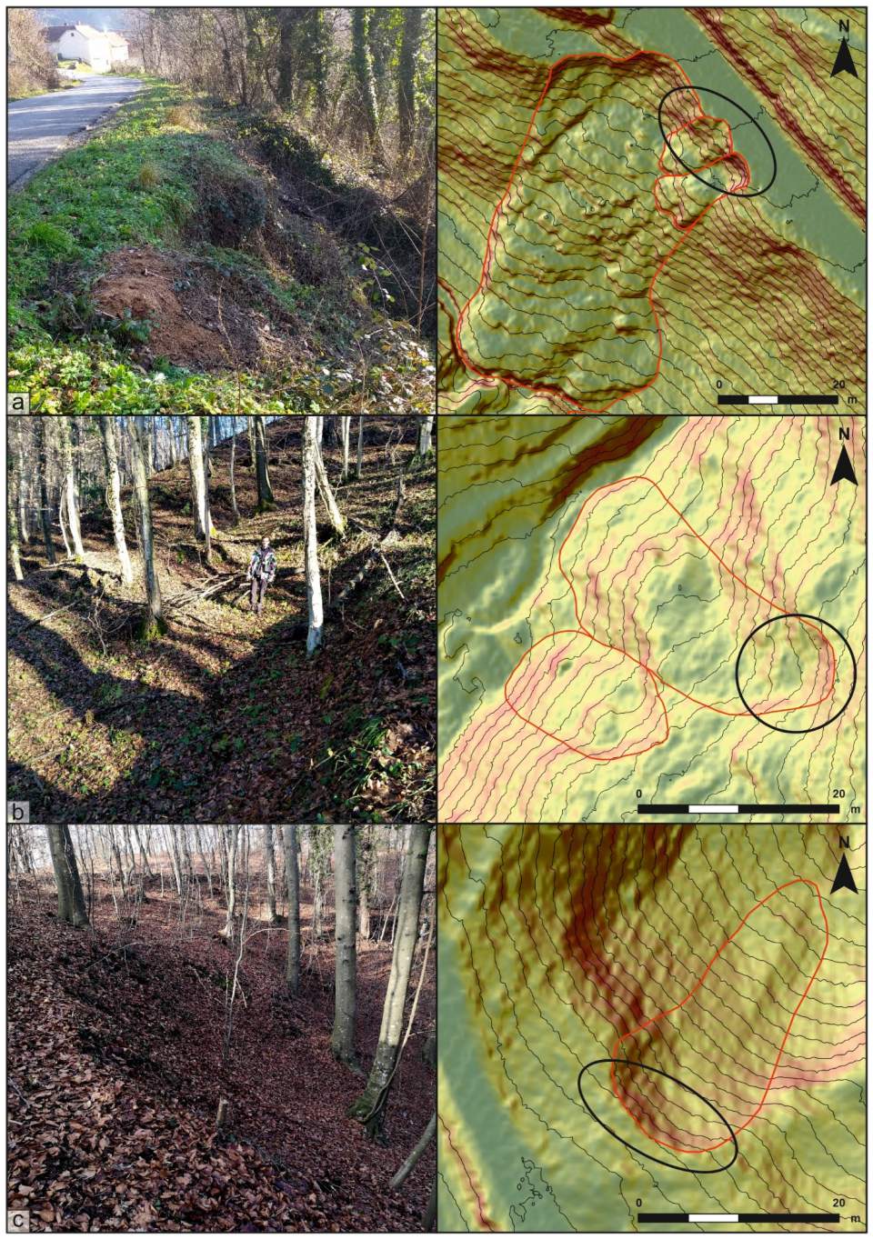
The topographic derivative datasets, derived from LiDAR DTM 0.3 m resolution, used to interpret the landslide morphology were: hillshade maps with different sun azimuth angles of 315°, 135°, and 45° and a constant altitude angle of 45°, slope maps, and 0.5 m contour lines. In addition, orthophoto images from 2014–2016 were used to check the morphological forms along roads and houses, such as artificial fills and cuts, similar to landslides on DTM derivatives. Landslide identification on the LiDAR DTM derivatives was based on visual interpretation of landslide features (e.g., concave main scarps, hummocky landslide bodies, and convex landslide toes). The mapping was performed at a large scale (1:100–1:500) to ensure the correct delineation of the landslide boundaries. As a result, each mapped landslide polygon was assigned with the confidence of landslide identification. The confidence in landslide identification was expressed as ‘high confidence’, where the landslide parts and morphology are clearly visible and easy to interpret, and ‘low confidence’, where the landslide parts are not clearly visible or missing and the landslide morphology is unclear [34,35]. Additionally, remediated landslides were not mapped because on the 0.3 m LiDAR DTM was impossible to identify the typical landslide morphology. Visually interpreted landslides on LiDAR DTM derivative maps were field-checked in December 2021 and January 2022 (Figure 2). However, systematic field mapping of all landslides from the inventory could not be carried out due to a relatively large area of the entire pilot area (20.2 km²) and impassable parts of the terrain (neglected and overgrown land parcels).

3.3. Deriving Input Data Layers for Landslide Conditioning Factors and Elements at Risk

Ref. [5] states that landslide conditioning factors are not a prescribed uniform list, and their selection differs due to several factors [64]. For that reason, landslide susceptibility assessment input data layers were selected considering the scale, the purpose, suggested methods, and available data, and expertly based on the study area conditions. Moreover, according to [5], most of the conditioning factors presented in this study are highly applicable for large-scale landslide susceptibility assessments. Examining the study area as a part of landslide inventory verification and considering the application of the results, which are land-use spatial planning, special attention was given to anthropogenic conditioning factors. A total of 16 data layers for deriving landslide hazard assessment input data were selected and grouped into four categories: geomorphological, geological, hydrological, and anthropogenic (

Table 3. Source of input data layers for landslide hazard assessment in the study area.

Group	Source	Input Data Layer for Landslide Hazard Assessment
Geomorphological factors	25 m EU-DEM 10 m SGA DEM HR-LiDAR DTM	Elevation Slope gradient Slope orientation Terrain curvature Terrain roughness Terrain dissection
Geological factors	Basic Geological Maps (OGK) 1:100,000 HR-LiDAR DTM	Lithology (rock type) Geological contacts
	Basic Geological Maps (OGK) 1:100,000	Faults
Hydrological factors	25 m EU-DEM 10 m SGA DEM HR-LiDAR DTM	Drainage network Topographic wetness
	Topographic Map of Croatia 1:25,000 (TK25) Croatian Basic Map 1:5000 (HOK)	Springs Permanent and temporary streams
Anthropogenic factors	Sentinel-2 orthophoto imagery Digital Orthophoto Map (DOF) 1:5000 HR-LiDAR point cloud HR-LiDAR DTM Corine Land Cover Open Street Map (OSM) Land-use planning maps	Land-use Buildings Roads

). Data preparation and digitalization for all four groups of input data layers were performed in a wider study area. As a result, a larger extent of vector data, such as roads, faults, and streams, was used to derive proximity factor maps. In addition, the spatial distribution of input data on a wider area enabled the proximity classes to be more accurate.

The geomorphological group of input data layers includes elevation, slope gradient, slope orientation, curvature, roughness, and terrain dissection. The elevation map is defined as raw DTM, used to prepare slope gradient, slope orientation, contour, and curvature map using Slope, Aspect, Contour, and Curvature tools in the 3D Analyst toolbox. Geomorphometry and Gradient Metrics Toolbox v2 [65] were used to apply the Surface Area Ratio and Dissection tool, which resulted in the roughness and terrain dissection conditioning factors, respectively.

The preliminary analysis showed deviations in geological contacts on the Basic Geological Map [44,45] in the geomorphological environment visible on the slope-hillshade map. Field verification of the Basic Geological Map confirmed that the deviations are significant and cannot be neglected. Moreover, in many landslide susceptibility assessments, stratigraphic units presented in geological maps are aggregated and used to describe rock characteristics [66], that is, forming engineering geological formations. Therefore, engineering geological formations were additionally mapped using LiDAR DTM derivatives to modify the geological contact, according to a suggestion by [67,68]. The suggested methodology demonstrated efficacy in forested areas and resulted in an engineering geological map. After the visual interpretation of LiDAR DTM derivatives, the engineering geological units and their contacts were chosen as the landslide input data. Faults were obtained by digitizing the Basic Geological Maps since their deviation is difficult to estimate by both field surveys and map comparison.

The hydrological group of input data layers consists of a drainage network, springs, permanent and temporary streams, and topographic wetness. The drainage network was derived using DTMs following the ArcGIS 10.8 tools procedure: (i) Fill, (ii) Flow Direction, (iii) Flow Accumulation, (iv) Greater Than, (v) Stream Link, (vi) Stream Order, and (vii) Stream To Feature. Different variations regarding constant values in step iv were tested, and validation was performed visually by overlaying the drainage network over a hillshade map. By observing the drainage network density, the average distance between different network orders, and the morphological fitting of the network on the convex and concave parts of the slope, we were able to determine the optimal solution subjectively. The topographic wetness was derived using DTMs as input for the Compound Topographic Index (CTI) tool available in the Geomorphometry and Gradient Metrics Toolbox v2 [65]. Springs and temporary and permanent streams were obtained by digitizing the available topographic map on a scale of 1:25,000. Two types of input data layers were selected: (i) permanent streams, which represent more particularly defined information, and (ii) permanent and temporary streams, which represent all streams, that is, water flows in the study area.

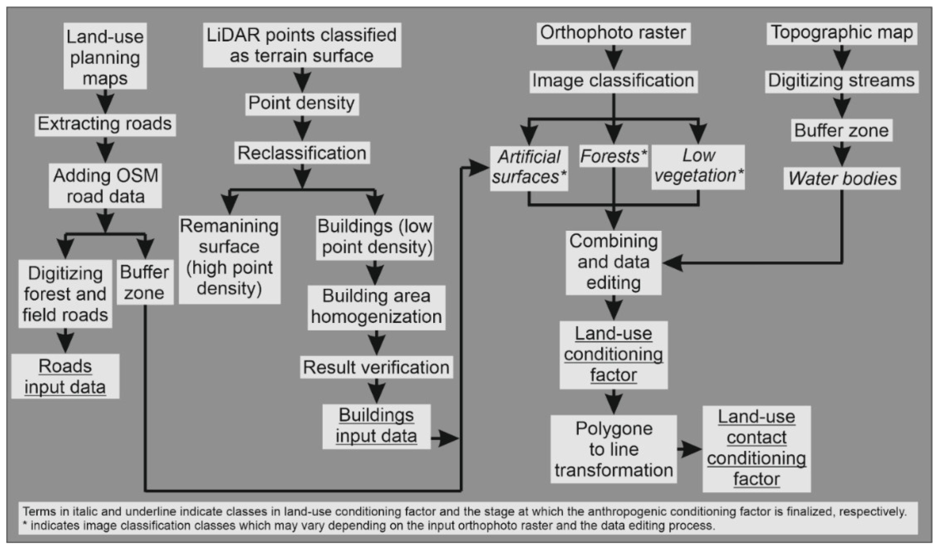
Anthropogenic input data layers were the most demanding to derive as they required four different input data sets and different processing methods, as shown in Figure 3. Starting from the LiDAR points, reaching robust buildings as a raster file is not an unambiguous process. Getting satisfactory results using verification to determine homogenization quality can differ depending on the LiDAR classification quality. Tools such as Focal statistics and Smooth in ArcGIS 10.8 and selecting vector files by their surface area allow a significant upgrade from the preliminary results after the reclassification stage. In the end, manually adding and removing buildings in the verification stage remained necessary to finalise input data. Considering the previous steps, this is achieved by overlaying the buildings on an up-to-date, high-resolution SGA orthophoto where buildings are well distinguished.

Official city and municipality land-use planning maps present the most detailed source of information about roads and traffic infrastructure. However, since the availability depends on each administrative unit, the best alternative is OSM road data [60]. Therefore, after extracting the roads from the official land-use planning maps [42,43], OSM roads were added to supplement the data in a populated area. Furthermore, to complete the road network, the forest and field roads in unpopulated areas were digitized on a hillshade map and up-to-date orthophoto imagery WMS [59].

The land-use input data layer is the most complex to derive as it usually consists of artificial areas, agricultural areas, forest areas, and water bodies. Applying an Image classification tool in ArcGIS 10.8 on high-resolution orthophoto imagery enables the creation of a raster file consisting of several classes. Since the only water bodies in the study area are relatively small streams, they are indistinguishable on the SGA orthophoto and had to be acquired using a different input map. After prospecting the study area using available data layers presenting water bodies, the topographic map on a scale of 1:25,000 [56] was used for digitizing streams that were buffered to an estimated width, presenting the water body class in the land-use data layer. Artificial surfaces consist of the building data layer and the buffer zone around road data layers, combined with the image classification results. The study area is low urbanized, so artificial surfaces are relatively small, and successful sampling for image classification was challenging. After successfully preparing individual classes of the land-use input data, the combining and data editing process consisted of homogenising the classes, that is, aggregation using the tool Focal statistics in the ArcGIS 10.8 software. Additionally, manual corrections were needed on the parts of the terrain where the previous methods showed poor results because of data preparation for landslide hazard assessments on a large scale.

The correlation between landslides and morphometric factors (elevation, curvature, roughness, dissection, and slope orientation), geological factors (lithological units based on the Basic Geological Map 1:100,000 and engineering geological units interpreted from LiDAR DTM), hydrological factors (drainage network and topographic wetness), and anthropogenic factors (land-use) derived from different input data sources is analysed and expressed through landslide percentage for each factor class. By comparing the area distribution of each factor map class and the landslide presence, that is, landslide number, it is possible to analyse the influence of the quality and resolution of input data on the accuracy and precision of landslide hazard assessment on a large scale.

4. Results

4.1. Landslide Inventory Map

In the study area in Hrvatsko Zagorje, initially, 904 landslides were identified and mapped on a scale of 1:100 to 1:500 on the LiDAR DTM derivatives. During the winter period in 2021/2022, 24% of the randomly selected landslides were checked on the field. From the 214 checked phenomena, 20 phenomena were rejected as landslides. Additionally, 28 phenomena were mapped in the field and added to the inventory, making the total number of landslides in the inventory 912 (Figure 4). Regarding the reliability of all mapped landslides, 525 landslides (58%) were identified as ‘high confidence’, and 387 landslides (42%) were identified as ‘low confidence’, that is, preassumed landslides.

During field verification, 4.9 km² or approximately 25% of the study area was checked. Of 912 interpreted landslides on LiDAR DTM, 24% or 222 randomly selected landslides were verified. A total of 163 verified landslides i.e., 73% were evaluated with ‘high confidence’ of visual identification on LiDAR DTM, and 59 or 27% landslides with ‘low certainty’ (Figure 5). Field checking resulted in 168 confirmed landslides (76%) and 35 presumed landslides (16%) based on hummocky morphology, while 19 landslides (8%) were not accessible due to neglect and overgrown land parcels. Furthermore, results from field checking were compared with the confidence of visual landslide identification on LiDAR DTM and 128 or 76% of confirmed landslides were evaluated with ‘high confidence’. In total, 35 landslides preassumed and not accessible during field checking were evaluated with ‘high confidence’, while 14 preassumed landslides and 5 inaccessible landslides were evaluated with ‘low confidence’ on LiDAR DTM. Most landslides can be dated as recently (re)activated due to the sharp appearance or a high degree of preservation of the landslide morphology. Therefore, the landslide inventory map of the study area represents a combination of seasonal inventory, landslides (re)activated in the winter of 2012/2013 and March 2018 [39], and historical landslide inventory.

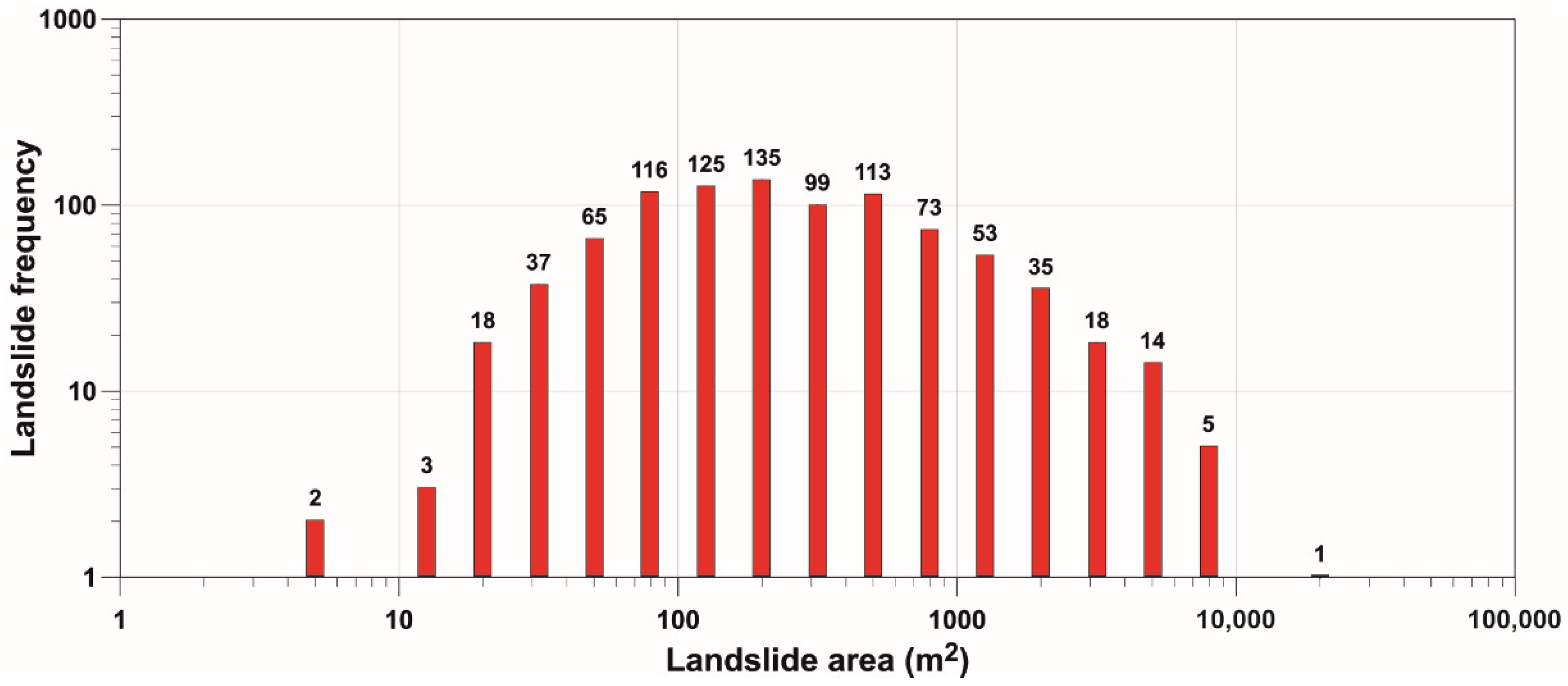
The total area of mapped landslides is 0.408 km² or 2.02% of the study area. The mean landslide density is 45.1 slope failures per square kilometre. The size of the recorded landslides ranges from a minimum value of 3.3 m² to a maximum of 13,779 m², whereas the average area is 448 m² (median = 173 m², std. dev. = 880 m²). The most frequent landslides in the inventory have an area of approximately 200 m², and almost 85% of the landslide bodies show a size between 40 and 2000 m². The small size of the landslides results from geological conditions (mainly Miocene marls covered with residual soils) and geomorphological conditions, where the differences between the valley bottoms and the top of the hills are rarely higher than 100 m [69].

The frequency–size distribution of all mapped landslides in the pilot area (Figure 6) shows two scaling regimes: a positive power-law scaling for small landslides and a negative power-law scaling for medium and large landslides. The transition between the positive and the negative power-law relations can be used to distinguish between small and medium landslides. Based on the rollover at approximately 200 m², 48% of the mapped landslides are small (<200 m²), and 52% are medium and large (>200 m²) in size. The prevailing dominant type of landslides are shallow soil slides.

4.2. LiDAR DTMs

Results of a quantitative assessment for 15 LiDAR DTMs derived in three raster resolutions (1, 2, and 5 m), using five interpolation methods, and 0.3 Kriging LiDAR DTM used for landslide inventory mapping, 10 m SGA DEM and 25 m EU-DEM, are presented in

Table 4. Comparison of DTM statistical parameters for the study area.

Interpolation Method	Resolution	Min	Max	Mean	St.Dev.	MAE	RMSE
Inverse Distance Weighted	1	119.57	682.54	304.46	77.35	1.99	137.81
	2	222.39	681.64	304.45	77.35	3.22	176.55
	5	224.41	680.03	304.45	77.35	6.02	242.82
					SUM	11.40	555.19
Natural Neighbor	1	119.59	682.29	304.72	78.01	1.98	137.81
	2	222.40	681.70	304.98	78.64	3.21	176.55
	5	222.41	680.02	305.75	80.44	6.18	242.82
					SUM	11.38	557.19
ANUDEM	1	222.44	682.10	304.45	77.36	2.00	137.81
	2	222.60	680.94	304.41	77.29	2.44	146.40
	5	223.00	679.93	304.43	77.32	7.05	252.57
					SUM	11.50	536.78
Kriging	1	222.30	682.59	304.45	77.35	1.70	128.27
	2	222.39	682.58	304.45	77.34	3.16	175.38
	5	222.76	679.82	304.42	77.31	5.51	228.35
					SUM	10.37	532.00
Local Polynomial	1	222.32	682.73	304.45	77.34	1.70	128.27
	2	222.51	680.95	304.38	77.21	2.39	146.40
	5	222.50	679.84	304.42	77.31	5.51	228.35
					SUM	9.60	503.01
Kriging	0.3	116.77	682.77	304.45	77.35	0.27	50.11
SGA DEM	10	222.25	680.79	304.72	77.23	12.89	334.40
EU-DEM	25	226.72	679.71	311.48	78.18	38.56	291.50

. Interpolation of high point density las point cloud to lower resolution LiDAR DTMs induces smoothing of the extreme values, causing similar results and almost negligible differences in minimum, maximum, mean (μ), and standard deviation (σ) values. Apparent exceptions regarding the lowest minimum values are present for 1 m IDW and natural neighbor DTMs due to a few pixels with significantly lesser values than in other DTMs. Moreover, the standard deviation and mean values in the natural neighbor interpolation show slightly higher values (σ = 78–80.4; μ = 304.7–305.8) compared with the other interpolation methods’ stable values (σ = 77.2–77.4; μ = 304.4–304.5). For all interpolation methods, minimum and maximum values reach their lowest, that is, highest values, in the 1 m resolution.

The n value (Equation (3)) for the MAE and RMSE analyses was 45,140. As expected, the MAE and RMSE values generally increase in lower resolutions. Local polynomial and Kriging interpolation methods show similar MAE and RMSE values, lower than the other interpolation methods. The highest difference between the local polynomial and Kriging interpolation was for the 2 m resolution, where MAE and RMSE of the local polynomial are lower and somewhat similar to ANUDEM values. Observing the sum of the MAE and RMSE values, the local polynomial interpolation method proved to be the most accurate, with the lowest values. IDW, natural neighbor, and ANUDEM showed similar results in the MAE values, somewhat higher than for a Kriging interpolation. Considering RMSE values, IDW and natural neighbor interpolation methods have the highest values compared to the local polynomial interpolation.

The 0.3 m Kriging DTM resulted in minimal MAE and RMSE values due to its high resolution. As expected, 10 m SGA DEM has significantly higher MAE and RMSE values compared with the 5 m LiDAR DTMs. The RMSE analyses for the 25 m EU-DEM resulted in a lower value than for a 10 m SGA DTM. However, the MAE value for 25 m EU-DEM is the highest among all analysed DTMs.

The 15 LiDAR DTMs in resolutions 1, 2, and 5 m derived using five different interpolation methods, 0.3 m Kriging LiDAR DTM, 10 m SGA DEM, and 25 m EU-DEM (URL-3) were used to produce slope gradient maps. The slope maps were classified into 5° classes and overlain with the landslide inventory map of the study area (Figure 7). The five interpolation methods (Figure 7A–E) are characterised by: (i) similar trends regarding slope classes and landslide area distribution; (ii) slight differences between different resolutions; (iii) the highest area percentages in lower (<10°) and higher (>30°) slope classes for the 1 m resolutions and the highest area percentages in 10–30° classes for 5 m resolutions; (iv) the most significant differences in slope classes between different resolutions present in 15–20° and 20–25° classes; (v) landslide area percentage showing minimum differences in the 0–5° and 25–30° slope classes; (vi) landslides being mostly present in the 15–20° slope class; (vii) landslide presence in 5 m resolution slope map being predominant in the 10–35° range, and least present in the <10° and >35° classes; (viii) the percentage of landslides and slope classes in the >60° zones being neglectable; (ix) landslide percentage steeply increasing until 15–20° class, compared with a mild decrease trend following, reaching a minimum at 60°.

The 10 m SGA DEM shows similar slope class areas and landslide area distributions compared with the 5 m LiDAR DTMs. On the other hand, 25 m EU-DEM depicts the most extreme values, with the most abundant slope class being 5–10°, reaching nearly 35% in landslide area and slope area distributions. Moreover, the 0–5° class of 25 m EU-DEM includes almost 10% of landslide areas, whereas, in all other scenarios, the 0°–5° class contains around 2.5% or less of the landslide areas. The 0.3 m Kriging LiDAR DTM has the most gentle decreasing trend in slope class distribution and the lowest maximum value of landslide presence in the 15–20° slope class (15%).

Overall, the comparison of slope class and landslide area distributions for different resolutions and interpretation methods shows that the resolution of DEM is the most significant factor and, consequently, has an important impact on a landslide hazard assessment. Therefore, considering minimal differences in the slope class area and landslide area distribution between interpolation methods, the relatively lowest values of MAE and RMSE parameters, the local polynomial interpolation, was chosen as the optimal method for deriving landslide conditioning factors in 1, 2, and 5 m resolutions.

4.3. Input Data Layers and Elements at Risk for Landslide Hazard Assessment

4.3.1. Geomorphological Input Data Layers

Six landslide geomorphological factors were derived using local polynomial LiDAR DTM in 1, 2, and 5 m resolutions; 10 m SGA DEM; and 25 m EU-DEM. DTMs and DEMs were used to derive slope gradient, slope orientation, terrain curvature, terrain dissection, and terrain roughness map. A comparison of minimum, maximum, mean, and standard deviation values for five continuous geomorphological factor maps is given in

Table 5. Comparison of statistical parameters calculated from geomorphological landslide conditioning factors.

Input Data Layer	Statistical Parameter	Elevation	Slope Gradient	Terrain Curvature	Terrain Dissection	Terrain Roughness
1 m LiDAR DTM	min	222.32	0.00	−2860	0	1
	max	682.73	83.66	1699	1	9.05
	mean	304.45	19.71	−6 × 10−12	0.50	1.09
	st.dev.	77.35	11.22	13.51	0.13	0.11
2 m LiDAR DTM	min	222.51	0.00	−1464	0	4
	max	680.95	79.42	562	1	21.79
	mean	304.38	19.50	2 × 10−16	0.49	4.35
	st.dev.	77.21	10.90	9.67	0.14	0.39
5 m LiDAR DTM	min	222.51	0.00	−124	0	25
	max	679.84	71.46	142	1	78.63
	mean	304.42	18.95	7 × 10−17	0.48	26.99
	st.dev.	77.31	10.21	4.97	0.18	2.04
10 m SGA DEM	min	222.25	0	−27.62	0	100
	max	680.79	58.23	30.63	1	182.93
	mean	304.72	17.01	0	0.46	106.18
	st.dev.	77.23	8.93	2.38	0.20	6.30
25 m EU-DEM	min	226	0	−2.08	0	625
	max	681	44.80	3.20	1	880.80
	mean	311.04	10.79	2.58	0.46	642.32
	st.dev.	78.25	7.24	0.37	0.22	27.90

. Terrain elevation, slope gradient, and terrain dissection maps show minimum differences in the studied statistical parameters. In addition, terrain curvature parameters follow a gradually decreasing trend in values as raster resolution increases, whereas terrain roughness parameters gradually increase. The resulting geomorphological input data layers were classified as depicted in Figure 8A–E.

In total, four classes were defined for the elevation map using an increment of 25 m a.s.l., and setting two edge classes at <250 and >300 m a.s.l., 1, 2, and 5 m LiDAR DTMs show (nearly) identical values, for both area distribution classes and landslide presence. All three DTMs reach maximum landslide presence in >300 m a.s.l class, slightly more than in the 250–275 m a.s.l. class. Compared with the LiDAR DTM, the 10 m SGA DEM depicts lower differences in landslide presence and no differences in elevation classes area distribution, following the same trend. On the contrary, the 25 m EU-DEM has an increasing trend from first to last class, in both landslide presence and elevation classes distribution, reaching the maximum in the >300 m a.s.l. class.

The terrain curvature map was classified into six classes with a 0.5 increment. As a result, the class area distribution on LiDAR DTMs shows a high area percentage in the edge classes of terrain curvature and a lower area percentage in the middle classes (from −1 to 1). Additionally, the LiDAR DTMs show identical landslide presence distribution in all terrain curvature classes, reaching the maximum in the edge classes, that is, classes with values lower than −1 and higher than 1. On the contrary, terrain curvature derived from 25 m EU-DEM shows opposite class area distribution and landslide presence than LiDAR DTM terrain curvature with maximum values of landslide presence and class area distribution in the middle −0.5–0 class. Therefore, the terrain curvature from 10 m SGA DEM shows a more uniform landslide presence and class area distribution than LiDAR DTMs and 25 m EU-DEM.

The terrain roughness map was normalized by equal classification in 50 classes. For practical comparison, 50 equal classes were resampled into six classes, where the 6th class represents the merged class from the 6th to the 50th classes. Significant differences are present in the first roughness class, even between the LiDAR DTMs. A 1 m LiDAR DTM depicts maximum landslide presence and class area percentage in the 1st class, followed by 2 and 5 m LiDAR DTMs. On all three LiDAR DTMs, landslide presence and class area percentage values are gradually reduced, reaching minimum values in the 6th class. On the contrary, 10 m SGA DEM and 25 m EU-DEM show a more uniform distribution of landslide presence and class area percentage across all roughness classes. The 25 m EU-DEM has maximum values of landslide presence in the 1st and 6th classes, whereas the 10 m SGA DEM has minimum landslide presence in the 1st class and maximum in the 6th class.

The terrain dissection map was classified into five classes, with a 0.2 increment. All five studied DTMs and DEMs have similar distribution trends of landslide presence and class area percentage. For example, the 1 m LiDAR DTM shows minimum values of area percentage in all terrain dissection classes, except the middle class 0.4–0.6, where it is depicted with maximum value. Similarly, the 25 m EU-DEM shows the highest area percentage values in all terrain dissection classes except in the middle 0.4–0.6 class, where it depicts the lowest area percentage value compared with the other three LiDAR DTMs and SGA DEM. All derived terrain dissection maps show a gradual increase in landslide presence in the terrain dissection classes, starting from minimum values in the 0–0.2 class, reaching maximum in the middle 0.4–0.6 class, followed by a gradual decrease into minimum values in the 0.8–1 class.

The slope orientation map was classified into nine standard classes, that is, flat areas, north, northeast, east, southeast, south, southwest, west, and northwest. All five analysed slope orientation maps derived from DTMs and DEMs have similar distribution trends of landslide presence and class area percentage, with maximum values in the SW class and minimum values in the flat areas. An exception is the 25 m EU-DEM slope orientation map that shows lower landslide presence values in the SE and W classes and moderately higher values in the SW and S classes compared with the other LiDAR DTMs and 10 m SGA DEM.

Figure 9 presents derived geomorphological input data and close-up extents in the study area. Terrain curvature and terrain roughness maps seem less detailed than the rest of the landslide input data. However, all maps present detailed information about geomorphological settings by examining in a close-up view, that is, on a large scale. In general, maps present different relief settings, such as valleys, slopes, and hill ridges. Moreover, disturbed and nondisturbed terrain characteristics are visible, as well as sudden changes in the relief. Examining all maps, while giving extra attention to slope areas where landslides are likely to occur, it is visible that each map provides different information regarding the slope terrain, making the combination of selected geomorphological input data suitable for landslide hazard assessments.

Low slope gradient and terrain dissection values are highly represented in gullies and narrow valleys following main water flows. Moreover, low slope gradient values and continuous elevation values depict plains, larger valleys, and agricultural areas. Low terrain roughness values and close-to-zero values of terrain curvature maps are most widespread throughout the study area. However, examining the close-up extent of the terrain roughness map, the values drastically change on slopes, reaching maximum values near low slope locations. Likewise, terrain curvature values vary from low to high on slopes, depicting ridges and gullies. The morphological features of the terrain on the LiDAR DTM are sufficiently detailed to allow landslide hazard modelling on a large scale.

4.3.2. Geological Input Data Layers

Lithological units and faults were digitized from the Basic Geological Maps sheets Varaždin and Rogatec [44,45]. Due to the inexact contact of the two sheets, subjective interpretation of a few faults and chronostratigraphic units was performed to unify data for the entire study area extent. In total, seven chronostratigraphic units providing soil and rock information and 48.62 km of faults were digitized (Figure 10). The small scale of the Basic Geological Maps (1:100,000) leads to an inaccurate geological contact deviating up to several hundred meters from actual environmental conditions.

Therefore, LiDAR DTM derivatives, such as hillshade, slope, curvature, and roughness map, were used to modify chronostratigraphic units and interpret engineering geological units. Based on visual interpretation of LiDAR DTM derivatives, five engineering geological units were identified in the pilot area, namely, (i) alluvium sediments; (ii) slopewash and older talus; (iii) sands, sandstones, and sandy marls; (iv) limestones; and (v) dolomites and limestones (Figure 10). Based on the homogeneity of identified lithologies forming the engineering geological units, they represent the engineering formations [70]. The interpreted engineering formations are briefly described in

Table 6. Description of engineering formations interpreted from LiDAR DTM derivatives.

Engineering Formations		Description
Name	Label	Geomorphological Setting and Origin	Engineering Material		Area
					km2	%
Alluvial sediments	M, S, Gal	Soils in flood plains trans- ported by fluvial processes	Fine and coarse-grained soils	Silt, sand, gravel	2.36	11.7
Slopewash and older talus	MS, Cbd	Soils on slopes transported by sheet erosion and gravitation	Composite soil	Sandy silt with dolomite and limestone cobbles	1.88	9.3
Sands, sandstones, and sandy marls	S, Ss, SMs	Marine sediments and poorly cemented sedimentary rock	Coarse-grained soil, hard soil-soft rock	Sand, sandstone, sandy marl, clay	13.77	68.1
Limestones	Ls	Carbonaceous sedimentary rock; medium bedded to massive	Rock	Sandy limestone, marly limestone, calcareous marl	0.83	4.1
Dolomites and limestones	Dl, Ls	Carbonaceous sedimentary rock; thinly to thickly bedded and massive	Rock	Dolomite, limestone, dolomitic breccia	1.38	6.8

. Compared with chronostratigraphic units, the engineering geological units provide minimum deviations from the actual environmental conditions. Moreover, the spatial distribution of units’ mapped LiDAR DTM derivatives is more accurate and detailed, especially in the alluvium sediments. The Holocene alluvium chronostratigraphic class is robustly represented in more extensive valleys. In contrast, the engineering formation of alluvium sediments from the engineering geological unit map is depictable in narrow valleys and plain areas, mapped based on the slope class 0–5°, providing the needed spatial distribution and accuracy for landslide hazard assessment on a large scale. Slopewash and older talus are an engineering geological unit that was not mapped on the Basic Geological Map and represent engineering soils on slopes transported by sheet erosion and gravitation. The presence of slopewash and older talus deposits was confirmed during the field surveys, and it was possible to determine the contact on the LiDAR DTM derivatives, such as the roughness and curvature maps. Limestone engineering geological formation was mapped by observing an area with sinkhole presence, mainly in the eastern part of the study area, in correspondence with the Tortonian chronostratigraphic class. Dolomite and limestone engineering formation depict Triassic deposits in the northern part of the study area, mapped in more detail using LiDAR DTM derivatives (e.g., slope map), since the slopes built from Triassic dolomite and limestone are steeper than surrounding clastic engineering formations. Sand, sandstone, and sandy marl classes represent Burdigalian deposits mapped on the Basic Geological Map, following the previously mapped engineering formation units. Finalized geological input data layers consist of digitized chronostratigraphic units, geological contacts, and faults from the Basic Geological Maps; engineering geological units interpreted from LiDAR DTM derivatives; and the engineering geological unit contacts.

The lithology input data layers, that is, the chronostratigraphic units from the digitized Basic Geological Map and the engineering geological units interpreted based on LiDAR DTM, minimally differ considering area class distribution (Figure 11). Exceptions are slopewash and older talus sediments, which are not mapped on the Basic Geological Map. Regardless of the similar area class distribution, the difference in spatial distribution, that is, geographic accuracy, is significant, as shown in Figure 10. Both lithological input data layer maps show high landslide presence in the sand, sandstone, and marl class and none or minimal landslide presence in the alluvial sediments, limestone, and dolomite and limestone classes. The Basic Geological Map has more landslides than the engineering formations map in the sand, sandstone, and marl class. Moreover, the slopewash and other talus class have significant landslide presence considering the low area percentage of the class.

4.3.3. Hydrological Input Data Layers

Based on the topographic map on a scale of 1:25,000, 43 springs and 55.10 km of streams (Figure 12A) were digitized. All digitized streams were classified as permanent (19.57 km) and temporary (35.53 km) streams. After digitizing, the Smooth tool in ArcGIS 10.8 was applied to stream a polyline data layer. Smoothing decreased the rough edges and sudden direction changes caused by digitizing, leading to more representative environment conditions. As a result of digitizing, it was possible to derive two types of landslide conditioning factors: proximity to all streams and proximity to permanent streams.

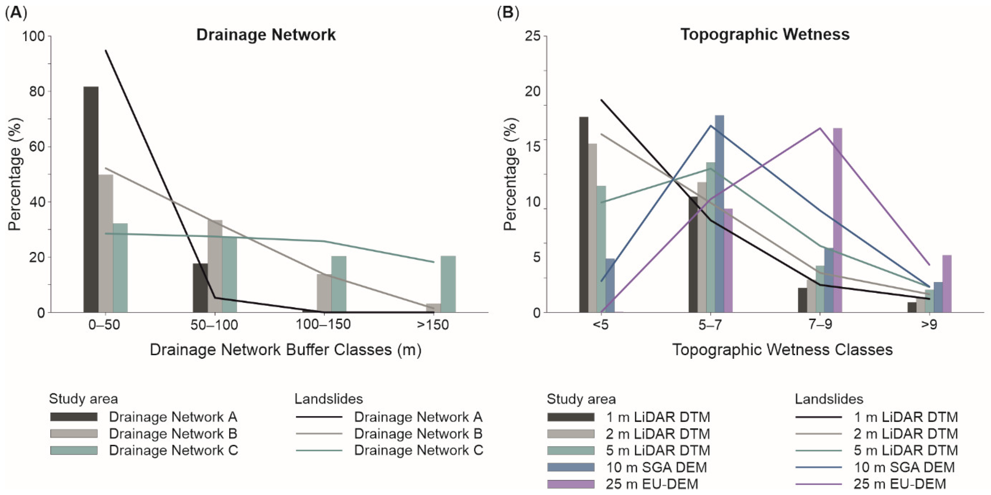
Figure 12B depicts topographic wetness derived from a 5 m LiDAR DTM of the study area, followed by a close-up extent. Hilltops and ridges are visible as areas with low topographic wetness values. The values increase on downhill slopes, reaching the maximum in gullies and valleys, whereas medium values are present on undisturbed slopes.

A topographic wetness input data layer derived in 1, 2, and 5 m resolutions resulted in uncategorical rasters with generally low differences in statistical information, except for minimum values (

Table 7. Comparison of topographic wetness statistical parameters derived from 1, 2, and 5 m LiDAR DTM, 10 m SGA DEM, and 25 m EU-DEM.

Input Data Layers	Topographic Wetness
	Min	Max	Mean	St.Dev.
1 m LiDAR DTM	−0.94	20.12	4.93	1.76
2 m LiDAR DTM	0.21	19.90	5.3	1.80
5 m LiDAR DTM	1.70	19.42	5.87	1.88
10 m SGA DEM	3.16	18.45	6.48	1.74
25 m EU-DEM	4.55	17.01	7.85	1.54

). 10 m SGA DEM and 25 m EU-DEM topographic wetness maps show moderate differences compared with the LiDAR DTMs, having relatively higher minimum and mean values and moderately lower maximum values. The most significant changes in statistical parameters are depicted when comparing the 1 m LiDAR DTM topographic wetness to the 25 m EU-DEM. An exception is the standard deviation value, where the most significant difference is between 5 m LiDAR DTM and 25 m EU-DEM.

The drainage networks (Figure 12C) were derived from 1, 2, and 5 m LiDAR DTMs. Visually examining the results and comparing the drainage networks, priority was given to the resolution that reflects actual environmental conditions in the best way. Finally, the 5 m resolution LiDAR DTM was used as the input for further deriving drainage network variations, depending on the methodology step iv Greater Than tool in ArcGIS 10.8 (Section 3.3), using three values for deriving different drainage network branchings. That is, the three selected options included constant values of 100, 500, and 1500, resulting in Drainage Network A, Drainage Network B, and Drainage Network C classes (Figure 12C). The necessity to iteratively test the options when deriving the drainage network is easily depictable in the close-up extent (Figure 12C), where Drainage Network A describes the gullies in distributed slopes, followed by losing much of the branching details in Drainage Network B, and finally describing only main water flows in valleys, that is, ignoring disturbed terrain in the slopes, in Drainage Network C. Drainage Network A contain 265 km of polyline data and a density of 13.1 km/km². In contrast, Drainage Network B includes 118 km of polyline data with a density of 5.8 km/km², and Drainage Network C has 72 km of polylines with a density of 3.6 km/km².

For further analysis, buffer zones of 50 m were derived around all three drainage network data layers. As a result, proximity to drainage network maps with four classes were defined and compared regarding class area distribution and landslide presence. Distribution trends (Figure 13) indicate that class area distribution follows the landslide presence in all four classes for all three proximity-to-drainage-network maps. In other words, high-class area percentage values result in high landslide presence and vice versa. Drainage Networks A and B depict steep and moderate decreases in the class area from the first 0–50 m to the last class of more than 150 m. On the contrary, Drainage Network C has a gentle decrease, that is, nearly equal class area distribution. All three proximity-to-drainage-network maps have the highest landslide presence in the class 0–50 m. Proximity-to-drainage-network map A has nearly 100% of landslides in the 0–50 m class, that is, reaching the minimum value in the 50–100 m class and having the classes 100–150 m and more than 150 m without landslides. Proximity-to-drainage-network maps B and C reach minimum landslide presence in the class of more than 150 m.

4.3.4. Anthropogenic Input Data Layers and Elements at Risk

Available information for deriving anthropogenic input data were: (i) 10 m Sentinel-2 orthophoto, (ii) 0.5 m SGA orthophoto, (iii) LiDAR point cloud and LiDAR DTM, (iv) Open Street Map (OSM), (v) land-use planning maps, and (vi) Corine Land Cover. A comparison of the 10 m Sentinel-2 orthophoto imagery and 0.5 m SGA orthophoto imagery on a close-up extent (Figure 14) demonstrated the importance of the orthophoto resolution for preparing data layers for landslide hazard assessments on a large scale. For deriving input data for landslide input data maps and elements at risk, Sentinel-2 orthophoto with low resolution makes buildings, roads, and other relevant information indistinguishable. On the contrary, the high-resolution SGA orthophoto provides reliable information about environmental conditions and the degree of urbanisation. In this study, SGA orthophoto in resolution 0.5 m enables verification of several derived input data and automated mapping of anthropogenic data, that is, building, roads and infrastructure, and land use.

Using LiDAR points classified as terrain, a point density raster (Figure 15A) was derived using the Point Density tool in ArcGIS 10.8. LiDAR point cloud with high average point distance exposed nonterrain surface. Using near-minimum point density value as a cut-off reclassification value resulted in a two-class raster. One class contained mainly buildings and a significant amount of small-area artefacts. The artefacts mainly presented areas of high-density vegetation where ALS captured a few or no terrain surface points, resulting in minimum point density values. Since most of these areas were smaller than the average building size, they were successfully removed by selecting polygons with a predefined minimum surface size. Results were verified with 0.5 m SGA orthophoto, and minimum changes were made to finalize the building data layer, such as removing excess areas and manually adding buildings. The used methodology provided automatic detection of most buildings with high precision on a large scale. As a result, 2017 individual building polygons were defined, ranging from 2 to 2620 m² and with a mean value of 63.12 m². Buildings were generally adequately located, and the process reduced manual digitizing. However, building boundaries are often irregular and show deviations from the actual building appearance on the SGA orthophoto. However, for creating input data maps for landslide hazard assessment, that is, deriving buffer zones for proximity to buildings, these deviations are neglectable. Furthermore, smoothing building polygons would solve the problem of boundary irregularity if the resulting data layer is used to define elements at risk in the presented study area.

Since the land-use planning maps of the City of Lepoglava do not contain roads, OSM roads were used. In combination with the road data layer from the land-use planning map of the Bednja Municipality, a draft version of the road data layer for the study area extent was derived. Prospecting the derived road data layer on SGA orthophoto showed low spatial deviation, that is, a satisfactory level of precision for large-scale landslide hazard assessment. However, further digitizing on orthophoto maps (Figure 15B) and hillshade (Figure 15C) was needed to complete the data since the prospection revealed unmapped roads in forested and low-populated areas. These mainly included forest pathways, unregistered roads, field roads, and similar, clearly visible on the hillshade map derived from 1 m LiDAR DTM and orthophoto imagery. Furthermore, applying the smoothing tool on the digitized road polylines increased the road curvature to actual conditions in the terrain. Therefore, the prepared road data layer for the subject study area can be used for further derivation of landslide conditioning factors and elements at risk. In total, 218.43 km of roads were identified, out of which 38.06 km are from the OSM (City of Lepoglava), 53.09 km of roads are from the land-use planning map of Bednja Municipality, and 127.28 km were digitized from high-resolution remote sensing data (Figure 15D).

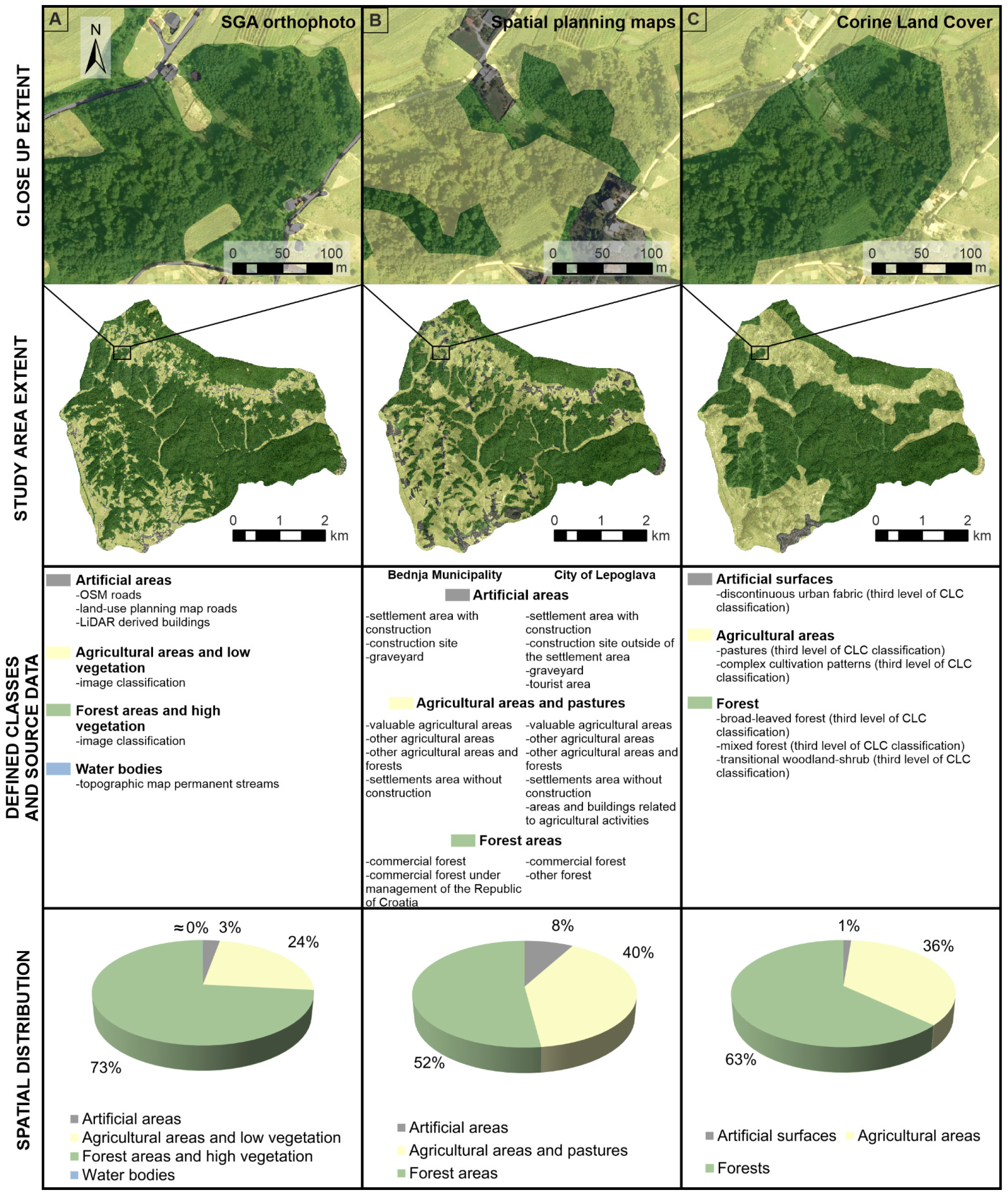
SGA orthophoto with a resolution of 0.5 m was prospected to determine which land use classes are possible to capture using the Image classification tool in ArcGIS 10.8 to derive land-use map A (Figure 16A) using the suggested methodology described in Section 3.3 (Figure 3). Moreover, the prospection provided the information on which colour combinations, that is, different samples, represent land-use classes. Considering the high resolution and quality of the SGA orthophoto, three land-use categories were defined, that is, agricultural areas and low vegetation, forest areas and high vegetation, and artificial areas. After verification of the resulting land-use map, it was concluded that two classes, agricultural areas and low vegetation and forest areas and high vegetation, show relatively high accuracy and precision, while artificial areas were mapped with reduced success. To minimise the manual editing and digitizing process, the sample-taking process for each land-use class was performed iteratively, visually prospecting the results after each iteration by comparing them to the SGA orthophoto imagery. Despite the optimization iterations, the process resulted in a significant amount of small polygons improperly classified. To address the issue and aggregate the final land-use classes of agricultural areas and low vegetation, and forest areas and high vegetation, Focal statistics and Selecting by area tools in ArcGIS 10.8 were used. The artificial area class was finalized by merging the building data and a buffer zone of the road data layer. Furthermore, the water bodies class was defined using the buffer zone around digitized permanent streams from hydrological input data layers. After finalizing all four land-use classes, data merging included verification of land-use boundary zones, that is, checking overlaps and gaps.

Land-use map B was derived using the most recent land-use spatial planning maps (Figure 16B) for the City of Lepoglava and the Bednja Municipality. The spatial planning maps consist of a large number of classes, which were generalized into four land-use classes to ease usage for landslide hazard assessment. After combining original spatial planning classes, the three final classes were artificial areas, agricultural areas and pastures, and forest areas (Figure 16B). The main problem on the derived land-use map is the artificial area, which is largely oversized, often including agricultural areas in the buildings’ immediate proximity. Moreover, the contact between the agricultural area and pasture class and forest area class deviates from the environmental conditions on high-resolution SGA orthophoto imagery. This resulted in agricultural area and pasture class overspread in the forest area class, which drastically influenced the spatial accuracy of the derived land-use map B in the study area.

Corine Land Cover (CLC) presents land use map C (Figure 16C). Considering large-scale landslide hazard assessment, all levels of classification showed little difference regarding land-use classes in the study area. Therefore, the first hierarchy level was selected for a representative CLC land-use map (Figure 16C). Regardless of the information details, the distribution of the land-use classes was unprecise, with extensive deviations from theactual environmental conditions. Unlike land-use map B, derived from current spatial planning maps, land-use C resulted in a relatively similar spatial distribution to our proposed methodology (land-use A). However, the deviations in land-use contact on CLC are even more severe than the spatial planning maps (land-use B map), which is expected considering the scale and the source of data used to prepare the CLC data layer. The CLC land-use map does not consist of roads or buildings in the artificial surfaces class, as it only captured discontinuous urban fabric at the very south of the study area. Moreover, the agricultural area class on CLC does not contain low vegetation pastures and valleys, which are well captured in land-use maps A and B. Land-use maps B and C provide too generalized and homogenous land-use class distribution compared with high-resolution SGA orthophoto imagery. Moreover, land-use boundary lengths between classes derived from land-use maps A, B, and C are 357.48, 233.64, and 55.73 km. Having the most extended contact length, land-use map A represents the optimal input data layer for preparing the anthropogenic landslide conditioning factors.

Land-use maps B and C show similar class area distribution and minimum landslide presence difference (Figure 17). On the contrary, land-use map A has moderate differences in class area distribution in the agricultural area and low vegetation class and forest area and high vegetation class compared with land-use maps B and C, and significant differences in landslide presence. Based on the conducted analysis, all three land-use data layers have the highest landslide presence in the forest area and high vegetation class. In the artificial area class, land-use maps A and C depict no landslide presence, whereas land-use map B shows a small landslide presence.

5. Discussion

5.1. Landslide Inventory Map Interpreted Based on LiDAR DTM Derivatives

Landslide inventory mapping for this study was performed on the LiDAR DTM derivatives for the 20.2 km² area in the Hrvatsko Zagorje region. Geomorphological mapping of the landslide inventory was inadequate because most landslides are located in forested and seminatural areas. The ability to follow a landslide boundary accurately in the forest is limited by the reduced visibility of the slope, a failure due to dense vegetation cover, the local perspective, the size of the landslide, and the fact that the landslide boundary is often indistinct [71]. Automated landslide mapping using vegetation cover algorithms or interpretation of landslides using SAR (Synthetic Aperture Radar) images is not possible due to dense vegetation cover and specific landslide morphology, that is, small and shallow landslides characterized by small displacements. LiDAR DTM enables a distant view of the slope and the landslide phenomena, which is preferable during landslide inventory mapping to reach better results, and a more accurate and complete landslide inventory map [25]. However, the accuracy of landslide inventories made by visual interpretation of LIDAR DTM largely depends on the researcher’s experience in landslide identification and mapping [72]. That is, certain practice and expertise in landslide identification on morphometric maps are needed to interpret the characteristic landslide morphology on maps derived from LiDAR DTM.

During the landslide inventory mapping, the landslide identification procedure was carried out several times for the entire study area. Each time, ‘new’ landslides were identified, which were not observed in the previous process of interpretation of a morphometric map derived from LiDAR DTM. Results from field checking were compared with the confidence of visual landslide identification on LiDAR DTM, and 76% of confirmed landslides were evaluated with ‘high confidence’. Based on the landslide identification confidence, percentage of confirmed landslides during field checking, and the landslide frequency–normal size distribution, it can be concluded that LiDAR DTM is a very useful tool for landslide mapping in the Neogen sediments of NW Croatia [35], despite the landside characteristics (small and shallow landslide bodies) and the dense vegetation cover (forested areas). Furthermore, the landslide inventory derived by visual interpretation of LiDAR DTM contains a representative number of all landslide sizes in the pilot area, which is necessary for a reliable landslide hazard assessment on a large scale.

5.2. LiDAR DTM for Landslide Susceptibility Assessment

Statistical parameters combined with the nearly identical slope histograms and landslide distribution indicate minimal differences between analysed LiDAR DTMs. However, in all interpolation methods, the 1 m resolution shows the highest value for the maximum and the lowest for the minimum parameter. The 0.3 m resolution Kriging DTM histogram confirms that higher resolutions enable reaching more extreme values and capture relief details in the study area more evenly. However, the quantity of landslide presence is different as the extreme values are lost, that is, losing the relief details due to lower resolution. Finally, the 25 m EU-DEM significantly deviates from the actual environment conditions compared with the LiDAR DTMs and 10 m SGA DEM.

The RMSE and MAE parameters were applied to determine minimum deviations of the interpolation methods. The 0.3 m Kriging LiDAR DTM resulted in the lowest RMSE and MAE values, utilizing the high-density points. However, LiDAR DTMs with a very high resolution will result in too fragmented landslide susceptibility zones in large-scale modelling. For that reason, 1 to 5 m resolution LiDAR DTMs should be used in a large-scale landslide hazard assessment depending on the average landslide size in the research area. Furthermore, considering the tested variations of the LiDAR data, we concluded that if the LiDAR data density matches the landslide hazard assessment scale, the selection of interpolation method for deriving LiDAR DTM will not have an influence. However, this would likely not be the case with limited and insufficient point density LiDAR data. Therefore, determining the minimum point density of LiDAR data for specific scales of landslide hazard assessment and deriving input data layers remain an open question.

5.3. Input Data Layers for Landslide Conditioning Factors and Elements at Risk

The geomorphological (elevation, slope orientation, terrain curvature, terrain dissection, terrain roughness) and hydrological (topographic wetness) input data layers derived from LiDAR DTM have the trend of minimum differences in mean and standard deviation values between resolutions. Based on the comparison of class area distribution for all geomorphological and hydrological input data layers, it can be concluded that there are significant differences between LiDAR DTMs and available 10 m and 25 DEMs because actual environment conditions are represented with significant limitations. Different resolutions and sources, that is, spatial accuracy of the input data, will affect the landslide susceptibility modelling because most statistical methods are based on landslide density in the conditioning factor class. In other words, different conditioning factor class areas and landslide densities in one of the landslide conditioning factor maps directly affect the estimated landslide susceptibility, which is especially pronounced in large-scale assessments. The influence of the input data spatial accuracy on the final susceptibility map should be the subject of quantitative analysis and further research.

Subjective interpretation of the only available geological data for the study area, the Basic Geological Map, leads to significant data loss and results in deviations from actual environmental conditions that should be avoided when conducting large-scale landslide susceptibility assessments. Using geological data from small-scale geological maps and information from the geological data sheets enables the researchers to get acquainted with the terrain and the geological settings. LiDAR data, that is, high-resolution DTM derivatives, enable distinguishing the geological settings in more detail, improving geological contacts, and aggregating chronostratigraphic units into engineering formation units, which are more suitable for landslide susceptibility assessments. The limitations of this approach could be the presence of different geological settings across the study area, in which engineering units cannot be distinguished from the LiDAR DTM derivatives. Moreover, field mapping as an alternative to small-scale robust geological data would be too time-consuming, and using only LiDAR DTM derivative maps alone cannot provide sufficient data. Without LiDAR DTM derivatives, the geological data on a scale of 1:100,000 could be used only for small-scale landslide susceptibility assessments. However, the process described in our study showed that combining small-scale geological maps and LiDAR DTM derivatives resulted in significantly reduced deviations from the actual environmental conditions, except for the geological structures, that is, fault data set. In our study area, in Hrvatsko Zagorje, it was impossible to map structural elements such as faults on LiDAR DTM derivatives due to the geological setting in which they are not clearly visible, that is, 93% of the study area is covered with Miocene and Quaternary sediments.

Streams displayed on the topographic maps on a scale of 1:25,000 are visible in the LiDAR DTM derivatives, such as hillshade maps. Moreover, streams on the LiDAR DTM derivatives sometimes can be similar to forest paths, and field checking is necessary. Additionally, the topographic map legend enables more information about streams, enabling their classification into permanent and temporary, which is impossible from the digitisation of LiDAR DTM derivatives. On the other hand, digitized streams from the topographic maps present higher-order flow in the drainage network, providing roughly five times fewer streams in length than the drainage network. For that reason, determining the robustness of input data is crucial to making it fit for the selected scale of the analysis. For example, comparing the three different drainage networks, we concluded that the scenario that manages to cover gullies in steep slopes without having the drainage network edges too close to each other should be considered optimal. However, testing the values of the buffer zones around the drainage network was not in the scope of this study, except for comparative purposes, and they should be further analysed because they could significantly impact the landslide susceptibility model. Therefore, combining small-scale topographic data and LiDAR DTM derivatives can provide optimal hydrological input data layers for landslide susceptibility assessment on a large scale. An exception is spring data that are impossible to map by the interpretation of LiDAR DTM derivatives and should be digitized from topographic maps.

Almost all roads (except forest roads and paths) in the study area are well distinguishable on the 50 cm SGA orthophoto imagery. However, available city and municipality land-use planning maps and OSM road data layers were used to reduce the digitising process. Furthermore, OSM data are satisfactorily precise but generally incomplete, missing buildings and roads in rural study areas. In that case, LiDAR point cloud and a hillshade map can be used to complement building and road data layers. The object-based classification of land-use classes depends on the quality of capturing the most common land-use classes, such as artificial surfaces and agricultural and forest areas. Moreover, the accuracy of the derived land-use data highly depends on the researchers’ ability to select necessary samples of each class on the orthophoto. We suggest prospecting the study area to determine the distribution of each class and in what manner each class is visible on the high-resolution orthophoto. The results are often heterogeneous and misleading, especially for agricultural and forest classes. We found that homogenizing the preliminary results to remove misleading polygons, to the extent that the data are still as heterogeneous as possible, provides the most detailed information for large-scale landslide hazard assessments. That is, artificial areas, agricultural areas and low vegetation, forest areas and high vegetation, and water bodies are the four defined classes, giving descriptions accordingly to the areas they cover, compared with the actual environment conditions presented in the orthophoto imagery. Streams and similar water bodies on LiDAR DTM derivatives often look similar to other natural shapes, such as gullies or forest paths, so we suggest prospecting the source files to mitigate the misinterpretation. In any case, spatial distribution can be misleading, as two different land-use maps could have a similar class area distribution, whereas their spatial distribution in the study area can deviate significantly. Applying the proposed method to derive building and road data layers and land-use maps from LiDAR data and high-resolution orthophoto images reduces the number of manual corrections needed in larger study areas. Moreover, the proposed methodology results in optimal input data considering the amount of detail and minimum deviations to the actual environmental conditions.

6. Conclusions

The preparation of input data and cartographic thematic layers is the most important and demanding step in the framework of landslide hazard assessment because all applied methodologies and derived results strongly depend on the quality of input data. Therefore, the input data for landslide hazard assessment on a large scale were prepared and analysed for the study area (20.2 km²) in Hrvatsko Zagorje (Croatia), where only limited medium-scale topographic and small-scale geological data are available.

The result of the visual interpretation of LiDAR DTM morphometric derivatives is the landslide inventory map, which consists of 912 identified and mapped landslides, ranging in size from 3.3 to 13,779 m² and with an average landslide density 45.1 landslides/km². Based on the normal distribution of mapped landslides and the assessment that 65% of landslides are reliably identified, it can be concluded that the inventory of visually mapped landslides for the study area of the 20.2 km² is detailed and complete. The prevailing landslide types are shallow and small to medium-sized soil slides that cause minor property and infrastructure damages. However, due to high landslide density, small and shallow landslides can cause significant damage on local roads in Hrvatsko Zagorje, and should not be neglected during landslide susceptibility analysis. Considering the preservation of landslide morphology throughout the study area, it can be concluded that most of the landslides in the inventory are recent and (re)activated by extreme hydrometeorological events in the winter of 2012/2013 and February 2018. The result is a combination of seasonal and historical landslide inventory, which are high-quality and representative input data for further landslide hazard assessment on a large scale. The quality of the inventory was also proved by field-checking, which confirmed the methodology of landslide identification and mapping as well as resulting high-quality inventory and its representativeness as input data for further testing of landslide conditioning factors and verification of the relative importance of factor classes.

Prior to deriving all the landslide conditioning factors, the analysis of how the interpolation method and resolution affect the quality of the LiDAR DTMs was performed. The LiDAR DTMs’ statistical parameters, the area distribution of slope map classes derived from LiDAR DTMs, and the landslide presence in slope classes showed that high-density LiDAR point cloud enables the derivation of high-quality DTMs at an appropriate resolution, regardless of the interpolation method. Furthermore, 15 LiDAR DTMs were compared with available DEMs, that is, 10 m SGA DEM and 25 m EU-DEM. As a result, 10 m and 25 m available DEMs significantly differ from LiDAR DTMs, considering landslide presence in slope class area distribution, indicating that they should not be used as input data for landslide hazard assessment on a large scale.

The high-resolution remote sensing data, LiDAR DTM, and orthophoto images are optimal input data sets for large-scale landslide hazard assessments because they enable the following: (i) derivation of geomorphological, geological, hydrological, and anthropogenic input data layers on a large scale, except geological structures and spring data; (ii) verification of input data layers; (iii) derivation of input data layers with the best fit to the actual environmental conditions (spatial accuracy testing); and (iv) efficient derivation of input data layers considering both price and time. Having representative spatial data depicting actual environmental conditions in the needed scale enables unambiguous selection of the optimal input data layers for landslide mapping, landslide susceptibility, and hazard modelling, as well as for the derivation of accurate data on elements at risk for landslide risk assessment. The resolution and spatial accuracy of input data layers for landslide hazard assessment, class area distribution of landslide conditioning factors, and landslide number in a single landslide factor class directly affect the susceptibility assessment in statistics-based models. Furthermore, for iterative processes, such as drainage network derivation or object-based image classification of land-use data, high-resolution input data used for verification enable optimization of the settings needed for the scale of the analysis. Moreover, when preparing geological data or mapping engineering geological units, the LiDAR DTM derivatives allow significant corrections of imperfections in the spatial accuracy of the robust small-scale geological information.

The presented research study in a relatively small study area (20.2 km²) in Hrvatsko Zagorje showed that the high-resolution remote sensing data provide a quick and affordable tool that enables derivation of the most commonly used landslide conditioning factors and elements at risk for landslide risk analysis on a large scale, regardless of geomorphological and geological settings and the degree of urbanization. Furthermore, high-resolution LiDAR data are the only possible solution for landslide inventory mapping in highly vegetated and unreachable areas, which can be applied in NW Croatia (approximately 7000 km²) based on similar geomorphological and geological characteristics and the landslide type. The LiDAR-based landslide inventory and all other landslide maps produced from landslide conditioning factors and elements at risk, derived from high-resolution remote sensing data, enable a high confidence level during the spatial planning system implementation.