
Comparison of Selected Mathematical Programming Models Used for Sustainable Land and Farm Management


Department of Agricultural Economics, Aristotle University of Thessaloniki, 54124 Thessaloniki, Greece
Land 2022, 11(8), 1293; https://doi.org/10.3390/land11081293
Submission received: 28 July 2022
/
Revised: 4 August 2022
/
Accepted: 9 August 2022
/
Published: 11 August 2022
(This article belongs to the Section Landscape Ecology)
Abstract
:The aim of this study is to compare three mathematical programing models used for sustainable land and farm management. The sample for the comparison was 219 agricultural holdings participating as beneficiaries of the measure ‘Modernization of agricultural holdings’ in the Rural Development Plan at the Region of Central Macedonia in Greece. Using the crop plan of the agricultural land of these farms the mathematical programming models calculate the optimum solution under different and conflicting goals. The results of the methodologies of Linear Programming (LP), of Positive Mathematical Programming (PMP) and Weighted Goal Programming (WGP), are compared in terms of the proposed agricultural land changes. The sustainability of farms is measured with the use of eleven economic, social, and environmental indicators. Each model has some unique advantages and disadvantages that can enable it to be implemented in particular situations. In the conclusions to this research the characteristics of each model are highlighted.
1. Introduction
There are many studies in literature regarding sustainable farm management, although in most cases it is examined as sustainability of agricultural holdings in relation to the implementation of various agricultural policies [1]. Additionally, mathematical programming models are frequently used in these kinds of studies as the proper methodological framework as they may be developed with a minimum amount of data and constraints in order to match the structure of such models [2,3,4,5]. Moreover, mathematical models increase farm management capabilities [6] and offer optimal solutions to important economic issues [7]. The majority of mathematical programming models are used mainly in combination with other approaches. In addition, Reidsma et al. [3] suggest that the sustainable farm management “needs to be based on farming systems analysis and integrated assessment”. By “integrated assessment” they mean an assessment that makes use of a number of combined mathematical models that are influenced by a number of different factors [8]. The mathematical programming models have been used in many studies for assessing the sustainability of farms by measuring several impacts [9,10,11,12,13,14], for policy changes [15,16] and other factors [17,18,19,20].
On the other hand, sustainable farm management is measured using various sustainability indicators. The literature review highlighted many attempts to record sustainability indicators. Bell and Morse [21] in their book Sustainability Indicators: Measuring the Immeasurable answer the problem if it is possible to measure what is difficult to measure. In their paper Pinar et al. [22] present the evolution of the FEEM (Fondazione Eni Enrico Mattei) Sustainability Index, a complex content, including 19 different indicators that are grouped into the three pillars of sustainability—economic, social, and environmental. To measure the farms’ sustainability many indicators have been developed. Many authors in various works [23,24,25,26] classify the sustainability indicators of agricultural holdings as follows: economic indicators (e.g., gross income, gross margin etc.); social indicators (e.g., family and foreign work); and environmental indicators (e.g., irrigation water use, use of nitrate fertilizers). Additionally, Gómez-Limón and Sanchez-Fernandez [27], in their paper, develop a practical methodology to assess the sustainability of agricultural holdings using composite indicators. Dantsis et al. [28] in their study combined 21 indicators expressed in one, in order to evaluate and compare the level of sustainability of agricultural plant production systems using a proposed methodology at the regional level.
Following the wide use of mathematical programming models for sustainable farm management, in this paper a comparison is made between different forms of mathematical programming methods. The comparison of different methodologies is very common in the literature [29]. In particular, the aim of this research is to compare the results in terms of economic, social, and environmental impacts, of three widely used mathematical programming methodologies: the first is the methodology of Linear Programming (LP) which is the most common approach of mathematical programming; the second is the Positive Mathematical Programming (PMP); and finally Multi-criteria Mathematical Programming solved as Weighted Goal Programming (WGP). The data for the comparison came from a sample of 219 farms participating as beneficiaries of the measure ‘Modernization of agricultural holdings’ in the Rural Development Plan at the Region of Central Macedonia in Greece. From the crop plans of these farms the average crop plan for the agricultural holdings was derived. The land changes in the average crop plan, after the implementation of each model, was the basis for our conclusions. Finally, the sustainability of farms was calculated using a set of eleven economic, social, and environmental indicators.
In the following section the literature review is presented. Section 3 describes the mathematical programming models used for comparison. The next Section 4 and Section 5 present the methodology used and the results obtained from the implementation of the models. The final section offers a set of conclusions.
2. Literature Review
Mathematical programming is the use of mathematical models, particularly model optimization, to aid decision making. Bradley et al. [30] present mathematical programming in their book as one of the best developed and most used branches of management science. It is the optimal allocation of limited resources, among competing activities, according to a set of constraints imposed by the nature of the problem under study. These constraints could reflect economic, technological, marketing, organizational, or many other issues. In general, mathematical programming can be defined as a mathematical representation, aimed at planning or designing the best possible allocation of limited resources.
2.1. Linear Programming (LP)
Linear Programming was first used as a method of maximizing or minimizing an outcome with the limited means available during the Second World War, and used for war purposes. Linear Programming, in its simple form, is a mathematical method that gives a defined combination of production factors and maximizes the economic result of the exploitation, subject to a set of constraints [31]. More specifically, Manos and Papanagiotou define Linear Programming in farm management [32] as the method that provides the best possible combination of production factors, that ensures the maximum total or per unit limited rate income or the minimum possible cost for the production. Linear Programming is used to organize new farms and reorganize old ones, with the goal of helping farmers achieve the maximum possible income or the minimum possible cost with a better use of existing inputs.
The use of Linear Programming is observed in several works in the Greek and foreign literature. For example, in his study Manos [33] uses linear mathematical programming to make economic use of available production factors and achieve a greater economic result, as well as to investigate the effect of changes in production factors and gross margin of production branches in the composition of the production plans and in the economic result of the whole region and its sectors. Rozakis et al. [34] in their study use a linear mathematical programming model to determine the optimal crop plan for each of the cotton farms they examine, maximizing the annual gross margin.
2.2. Positive Mathematical Programming (PMP)
Positive Mathematical Programming has been widely used in studies regarding sustainable farm management [35]; also, in recent years several variants of Positive Mathematical Programming have been developed and used in bioeconomic analysis [36,37,38]. These variations aim to overcome the limitations of the standard Positive Mathematical Programming approach and to improve the predictive ability of the models by using additional available information. In their study, Petsakos and Rozakis [39] integrate risks and uncertainty into the PMP approach. The same authors [40] compare two different PMP methods for their ability to predict changes in crop mix due to measures of decoupling and cross-compliance. Two different variants of Positive Mathematical Programming were also used by Kanellopoulos et al. [41] to evaluate the yield prediction of a general farm bio-economic model. A farm bio-economic model for farm level analysis was also developed by Janssen et al. [42] and Louhichi et al. [43]. Positive Mathematical Programming is widely used in the analysis of economic, social and environmental problems, in the context of the Common Agricultural Policy [44,45,46]. Arfini et al. [47] try to present a PMP model, suitable for estimating the variable cost of agricultural production linked to the different agricultural activities. This model was applied in three regions of Italy. Finally, Howitt et al. [48] in their work describe calibration methods for models of agricultural production and water use, where economic variables can directly interact with models of biophysical systems.
2.3. Weighted Goal Programming (WPG)
The complexity of decision systems, as well as the competitive conditions under which decisions are made, led to the development of the theory of Linear Programming with multiple decision criteria. The application of multi-criteria analysis (solving with the method of weighted goal programming) does not have as its sole objective the maximization of gross margin, as is the case in simple Linear Programming, but uses more than one criterion to find the optimal crop plan [49]. The model calculates the farmers’ utility function, considering various conflicting criteria, which seem to explain the producers’ decisions (e.g., maximizing farm income, minimizing risk, minimizing labor, etc.). In their paper Bournaris et al. [50] use multi-criteria mathematical programming to assess the effects of the measure “setting up young farmers”. Moreover, in the work of Manos et al. [51] a multi-criteria model was applied to study the impacts of tobacco decoupling on the income, employment of tobacco farmers, and also on the environment. In their work, Manos et al. [52] simulate the impact of different water price policies on agricultural production and analyze the economic, social and environmental impacts of alternative irrigation water policies using a multi-criteria analysis model. Bournaris et al., [53] present a fuzzy multi-criteria mathematical programming model, applied to an area of northern Greece with irrigated agriculture, where the optimal crop plan is achieved. Manos et al., [54] in their work, use a multi-criteria mathematical programming model to estimate the farmer’s utility function and simulate various scenarios and policies, as well as to synthesize alternative production plans. Additionally, Manos et al. [55] present a decision support system (DSS) in their work based on a multi-criteria optimization model. Its aim is to optimize the crop plan of the rural area considering the available resources. Finally, multi-criteria techniques with other methods have been used in such problems [56].
3. Mathematical Programming Models
Arriaza and Gómez-Limón [57] compared the predictive performance of various mathematical models (including PMP, LP and WGP), and using the production plans, crop yields, and gross margins of 18 farms over a five-year period; the optimal solutions of the mathematical models were compared with observed crop distributions after the 1992 reform of the EU’s Common Agricultural Policy. The following comparison of the results of the three Mathematical Programming methods is based on this work. In the following sections the mathematical models for the three mentioned mathematical programming methods are presented.
3.1. Linear Programming (LP) Model
In a linear programming problem with n variables and m linear constraints (equations or inequalities), we want to find the nonnegative values (≥0) of those variables that will satisfy those constraints and maximize or minimize some linear function of those variables.
We request the values of the variables xj that satisfy the following linear constraints:
and the non-negativities xj ≥ 0, j = 1, 2, …, n which give the maximum or minimum of the linear function
3.2. Positive Mathematical Programming (PMP) Model
Howitt [58] proposes a different perspective on mathematical programming, using more flexible specifications than the traditional linear constraints that, as mentioned, lead to the above problem. The Positive Mathematical Programming approach uses the farms’ existing crop plans to create self-calibrating models of agricultural production and resource use, consistent with microeconomic theory. The Positive Mathematical Programming approach is used to calibrate the model and guarantees the exact reproduction of the existing production plan without the use of additional calibration constraints that are difficult to justify in a manner consistent with existing economic theory [59]. One of the advantages of the method is that it achieves accurate calibration of linear programming models, even when there is a lack of sufficient data to choose appropriate constraints.
This model is a deterministic linear model, which maximizes the total gross margin of an average farm, given a set of policy and resource constraints [41].
where:
- z is the objective function,
- x is an n × 1 vector of production activities,
- r is an n × 1 vector of gross margins of production activities,
- c is an n × 1 vector of variable costs,
- A is an m × n matrix of technoeconomic coefficients,
- b is an m × 1 vector of output and policy constraints, and
- π is an m × 1 vector of the shadow values of factor constraints (e.g., marginal productivity of exhausted constraints).
3.3. Weighted Goal Programming (WGP) Model
Sumpsi et al. [60] and Amador et al. [61] proposed the methodology of weighted goal programming for the analysis and simulation of agricultural production systems based on multi-criteria techniques. The weighted goal programming methodology is used to study farmers’ decision-making.
The methodology of weighted goal programming can be summarized in three steps:
- Initially a set of objectives is determined that are considered the most important for farmers;
- Then the pay-off matrix of the above objectives is determined;
- Finally, the pay-off matrix is used to calculate a set of weights that optimally reflect farmers’ preferences.
Thus, the first step in our analysis consists of defining the set of objectives f1(X)… fi(X) fn(X) that represents the farmers’ true objectives (e.g., profit maximization, minimization of fertilizer use, minimization of labor use, etc.).
Table elements must be calculated by optimizing one objective in each row. Thus, fij is the value of the i-th feature when the j-th objective is optimized. When the payoff table is complete, we solve the following system of q (number of targets) equations:
where wj are the weights attached to each objective that reproduces the farmer’s real behavior, fij are the elements of the payoff matrix, and fi is the price achieved for the i-th objective, according to the existing crop plan.
Because the above system does not result in a set of wj it is necessary to search for the best possible solution, minimizing the sum of deviational variables that finds the closest set of weights. For this purpose, a weighted goal programming problem with percentage variable deviations is created [62]. This solution is found from the following linear programming model:
With restrictions:
where pi represents the positive deviation from target i and ni the negative deviation from it.
4. Methodology
The comparison for the selected mathematical programming methodologies follows the next procedure steps:
- For all farms the same crops were considered as the decision variables and the real situation crop plan is the same for all models;
- The same constraints were applied to all models;
- The objective functions of all models were optimized using the same goals. The goals were maximization of gross margin, minimization of fertilizers use, and minimization of labor use;
- All the optimum results for all models were compared to the real situation crop plan;
- Finally, a set of sustainability indicators (economic, social, environmental) is calculated to help the comparison procedure.
4.1. Real Situation
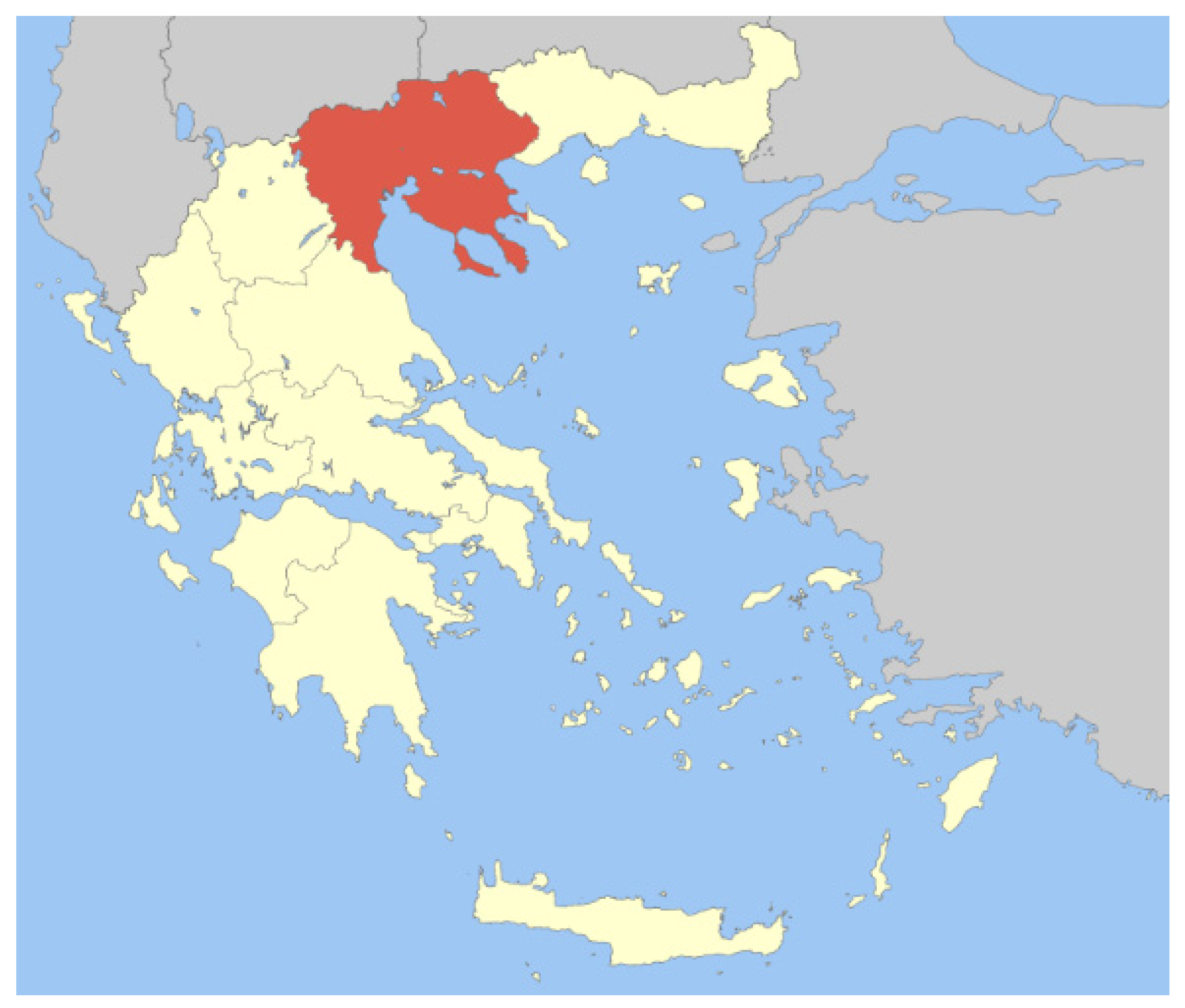
Among the thirteen Greek regions, the region of Central Macedonia is the one with the highest primary sector (Figure 1). According to the Hellenic Statistical Authority, the primary sector of the region corresponds to 22.6% of the total value of production in the country. The region includes seven regional units with different crop plans [63].
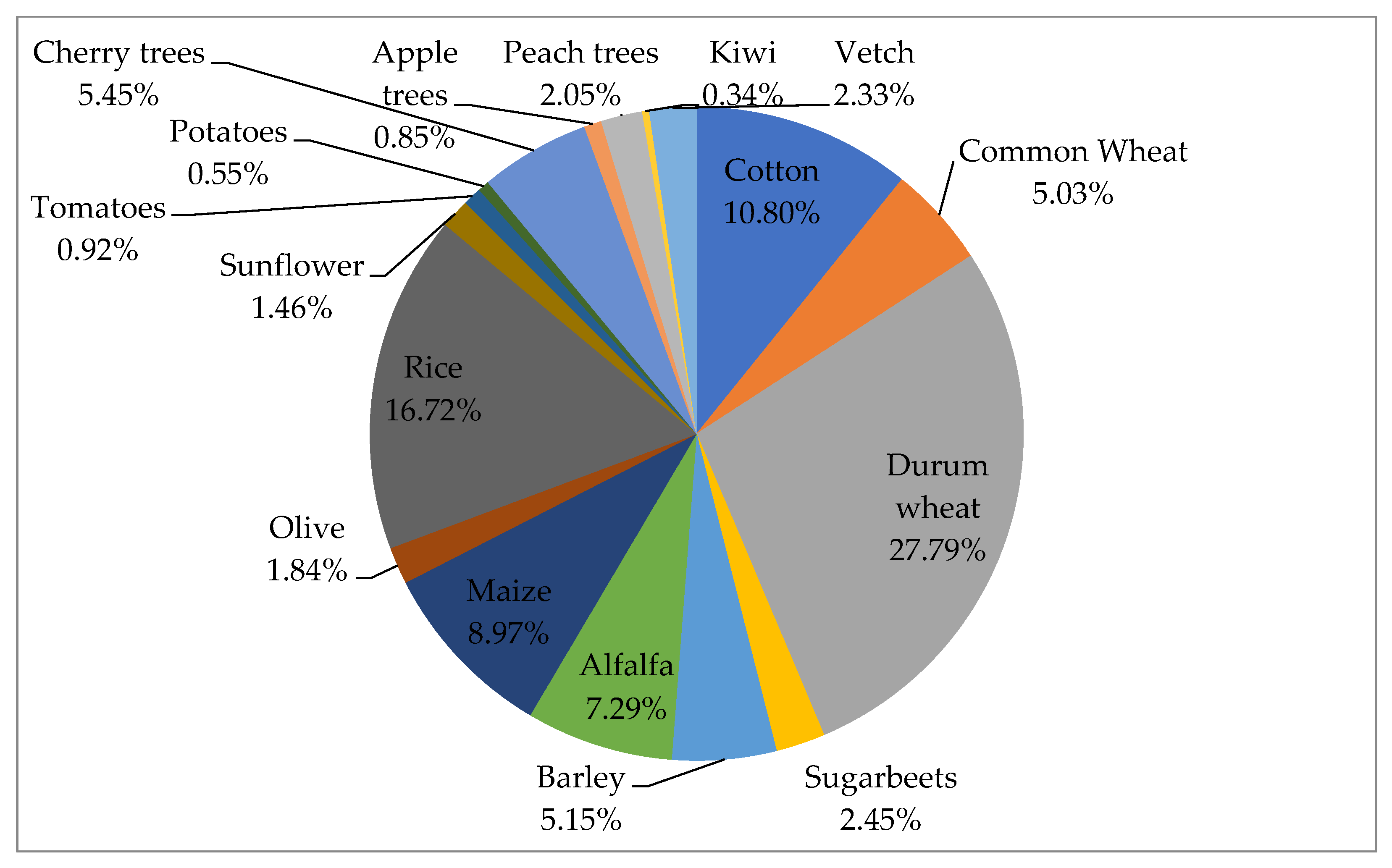
In Figure 2, the crop plan of the average farm of the sample is presented. The sample for the comparison was 219 agricultural holdings participating as beneficiaries of the measure ‘Modernization of agricultural holdings’ of the Rural Development Plan in the Region of Central Macedonia in Greece. The sample was obtained from a total of 5490 beneficiaries nationwide. Using descriptive statistical analysis, the average farm was derived.
The crop allocation to the crop plan is shown in percentage form, with the average crop plan equaling 100.
According to this data, durum wheat cultivation accounts for the largest percentage, or 27.79%. This is followed by rice and cotton crops, which have respective percentages of 16.72% and 10.80%. The cultivation of maize contributes to the crop plan by 8.97% and alfalfa by 7.29%. Cherry (5.45%), barley (5.15%) and common wheat (5.03%) crops have similar participation rates. Sugar beet (2.45%), vetch (2.33%), peach (2.05%), olive (1.84%) and sunflower (1.46%) crops follow with a smaller contribution. Tomatoes (0.92%), apple (0.85%), potatoes (0.55%) and kiwis (0.34%) crops contribute with a percentage of less than 1%.
4.2. Goals
The decision variables for the farmers were the crops (Xi) participating in the crop plan. The goals that we assumed reflected the farmers’ decisions were the maximization of gross margin:
the minimization of fertilizers use,
and the minimization of labor use
All these goals were introduced in the objectives’ functions of all models.
4.3. Constraints for All Models
For each of the three models, the same constraints are inserted in the mathematical programming matrix. The constraints used concern the land, the irrigated or non-irrigated area, constraints regarding the application of the CAP to each crop separately, market constraints for each crop, but also constraints for labor, variable costs and the fertilizers use. In detail:
Land: The sum of total available land for all crops (Xi) must add up to 100. This constraint is introduced to express the results of the models as percentages.
Irrigated Land: The total irrigated land must be less than or equal to the real total irrigated land of the region. Same constraints were inserted for non-irrigated land.
Labor use: The sum of required working hours (RWHi) for each crop (Xi) must be less than or equal to the total working hours (TWH).
Variable Costs: The sum of the required variable costs (RVCi) for each crop (Xi) must be less than or equal to the total available capital (TC).
Fertilizers use: The sum of required fertilizers (RFi) for each crop (Xi) must be less than or equal to the real crop plan fertilizers use (TF).
Other constraints: Market and agronomics considerations, such as rotation or CAP rights.
4.4. Indicators
Indicators are fundamental tools for measuring sustainability. The first major step towards identifying sustainability indicators to be taken towards achieving sustainability can be traced back to Agenda 21, an action plan launched at the United Nations Conference on Environment and Development (Earth Summit) in Rio de Janeiro 1992 (United Nations Conference on Environment and Development (UNCED, 1992). Since UNCSD’s initial effort, a plethora of sustainability indicators have been developed. Many of the indicators we might want to calculate are not available in some areas due to a lack of data. The chosen economic, social, and environmental indicators have been considered in practice, as they represent the balance between ideal indicators and the limitations imposed by the availability of data. The selected indicators are presented in Table 1. In the study, a total of 11 indicators (economic, social, and environmental) are examined. The economics were gross income and gross margin. Social indicators were labor use, annual work units, and seasonality [64]. Finally, six environmental indicators were examined, and they concern crop diversity, land cover, water use, nitrates use, electric and thermal power.
5. Results
For each mathematical programming method, the results are presented independently, and the final comparison of the methods is made using the sustainability indicators.
5.1. Results for Linear Programming (LP) Model
Table 2 shows the results and the changes made to the crop plan of the average farm after the implementation of the linear programming (LP) model. The main objective of the linear programming model was the maximization of the gross margin. The optimum solution gave an increase to gross margin by 5.6% from EUR 15,699 to EUR 16,573. The LP model did not achieve the other two goals of the study. The increase in the fertilizer use by 1.1% and the increase in the labor use by 1.2% were out of the expectations. Specifically, the fertilizer use increased from 6791 kg to 6867 kg. Accordingly, an increase in labor use was observed from 2715 h to 2748 h. The results data refer to the total average farm (100 acres).
The main result of the new crop plan is that three crops are planned to be abandoned (common wheat, sugar beet and vetch). In addition, a −47% reduction in cotton cultivation is proposed. More specifically, from 10.80 acres cotton reduced to 5.72 acres. All other crops show an increase and more specifically, the cultivation of durum wheat has increased by 19.8%, i.e., from 27.79 to 33.29 acres. Barley showed an increase of 30%, i.e., from 5.15 acres to 6.70 acres. Then, the alfalfa crop showed an increase of 20%, from 7.29 acres to 8.74 acres. Maize from 8.97 acres is proposed to have a participation of 10.76 acres, which was a 19.9% increase. The cultivation of olives increased in the new crop plan by 4.7%, i.e., from 1.84 acres to 1.93 acres. The cultivation of rice also increased, at a rate of 20%, from 16.72 acres to 20.07 acres. The sunflower showed an increase of 29.9%, i.e., from 1.46 to 1.89 acres. Tomatoes increased by 19.8%, from 0.92 to 1.10 acres. Potatoes increased from 0.55 to 0.67 acres, or 20.8%. Cherry trees showed an increase of 4.9%, i.e., from 5.45 to 5.72 acres. Apple trees increased from 0.85 acres to 0.90 acres, a percentage change of 5.4%. Peach cultivation increases in the new crop plan by 4.8%, i.e., from 2.05 acres to 2.15 acres. Finally, kiwifruits increased from 0.34 to 0.36 acres, i.e., by 4.9%.
5.2. Results for Positive Mathematical Programming (PMP) Model
Table 3 presents the changes made to the crop plan of the average farm after the application of the Positive Mathematical Programming (PMP) model. The main objective of the PMP model was to maximize gross margin. In fact, this goal was achieved, since the gross margin increased by 4.5%, from EUR 15,699 to EUR 16,398. The goal of minimization of fertilizer use was not achieved since there was an increase in the use of fertilizers from 6791 kg to 6801 kg, with a rate of 0.1%. On the other hand, labor use decreased from 2715 h to 2613 h, i.e., −3.8% achieving the third goal of labor use minimization.
In the optimum crop plan proposed by the PMP model, only sugar beet cultivation was planned to be abandoned. Six crops—cotton, common wheat, rice, sunflower, tomatoes, and vetch—decreased in the new crop plan. Specifically, cotton is reduced by 62.9% from 10.80 acres to 4 acres. Moreover, common wheat showed a decrease from 5.03 acres to 4.96 acres, i.e., a decrease of −1.5%. Rice cultivation decreased by 1%, from 16.72 acres to 16.55 acres. The sunflower and tomatoes crops showed smaller reduction rates with a decrease of 0.4% and 0.2%, respectively. Vetch exhibited a decrease at a rate of 1.3%, i.e., from 2.33 acres to 2.30 acres. All other crops increased their contribution to the new proposed crop plan. The cultivation of durum wheat increased by 16.9%, i.e., from 27.79 acres to 32.48 acres. Barley increased from 5.15 acres to 6.12 acres, or 18.7%. Alfalfa cultivation also showed an increase of 20%, specifically from 7.29 acres to 8.74 acres. Maize cultivation showed a similar percentage increase (19.9%), from 8.97 acres to 10.76 acres. Olive cultivation increased by 4.7%, from 1.84 acres to 1.93 acres. Potato cultivation showed a great increase of 20.8%, i.e., from 0.55 acres to 0.67 acres. Cherry cultivation increased at the same pace of 4.9% as kiwifruit cultivation. Cherry increased from 5.45 acres to 5.72 acres and kiwifruit from 0.34 acres to 0.36 acres. Finally, apple cultivation increased from 0.85 acres to 0.90 acres, i.e., by 5.4%.
5.3. Results for Weighted Goal Programming (WGP) Model
Table 4 displays the changes introduced to the average farm’s crop plan due to the implementation of the weighted goal programming (WGP) model. The three objectives of the WGP model were to maximize gross margin, minimize fertilizer use, and minimize labor use under one surrogate utility function. As shown in the following table, all three objectives were achieved. In fact, gross margin increased by 5.2%, fertilizer use decreased by 1.3%, and labor use decreased by 2.7%. In more detail, the gross margin from EUR 15,699 increased to EUR 16,511, when the fertilizer use from 6791 kg decreased to 6706 kg and the labor use from 2715 h decreased to 2642 h.
In the new crop plan the abandonment of three crops, cotton, common wheat, and sugar beet, is observed. All other crops showed an increase. In more detail, the cultivation of durum wheat showed an increase of 29.5%, i.e., from 27.79 acres to 35.98 acres. Barley cultivation increased by 30%, i.e., from 5.15 acres to 6.70 acres. Alfalfa also showed an increase, from 7.29 acres to 8.74 acres, i.e., by 20%. Maize increased by 19.9%, from 8.97 acres to 10.76 acres. The cultivation of olives showed an increase of 4.7%, from 1.84 acres to 1.93 acres. Rice cultivation increased from 16.72 acres to 20.07 acres, i.e., by 20%. Sunflower increased from 1.46 acres to 1.89 acres, i.e., by 29.9%. The cultivation of tomatoes increased by 19.8%, i.e., from 0.92 acres to 1.10 acres. Potatoes increased from 0.55 acres to 0.67 acres, 20.8%. Cherry trees showed an increase of 4.9%, i.e., from 5.45 acres to 5.72 acres. Apple trees showed an increase of 5.4%, i.e., from 0.85 acres to 0.90 acres. Correspondingly, peach cultivation also increased, from 2.05 acres to 2.15 acres, i.e., by 4.8%. Kiwis showed an increase of 4.9%, when from 0.34 acres they contribute to 0.36 acres. Finally, the vetch increased from 2.33 acres to 3.03 acres, i.e., by 30.2%.
5.4. Comparison of the Sustainability Indicators Results
Table 5 shows the changes of the main indicators during the application of the three models of mathematical programming. As regards the economic indicators in the real situation, the gross income is equal to EUR 29,499. After applying LP, the gross income increased to EUR 30,375 since when applying WGP, the gross income was equal to EUR 29,694, while when applying PMP, the gross income was equal to EUR 29,475. Regarding the gross margin, the real situation was EUR 15,699 but after applying the LP model it becomes EUR 16,573, and EUR 16,511 with the WGP model and EUR 16,398 with the PMP model.
The comparison of the three social indicators, those of labor use, annual work units and seasonality, shows the next results. The labor use in the real situation was 2715 h, and after the application of the LP model it increased to 2748 h, while after the application of the WGP and PMP models it decreases, respectively. The annual work units in the real situation were 1.55, when in LP it was 1.57, in WGP it was 1.51, and in PMP it was 1.49. Finally, seasonality in the real situation was 226.25, when there is an increase in the LP model and a decrease in the WGP and PMP models.
Table 5 also shows the changes of the six environmental indicators, those of crop diversity, land cover and water use, nitrate use, electric and thermal power. The crop diversity in the real situation was 17, while in LP, WGP and PMP it was 14, 14 and 16, respectively. In the real situation, the land cover was equal to 74.84%. Greater land cover is shown by the LP model, with 75.28%. while the WGP and PMP models show lower percentages of land cover, with 74.77% and 74.79%, respectively. The water use in the real situation was equal to 38,435 m3. The implementation of the LP model showed an increase in water use, while there was a decrease in the WGP and PMP models. Then, the use of nitrates in the real situation equals 6791 kg. It increases when applying the LP and PMP models, while when applying the WGP model a reduction was observed. The electric power was equal to 21.46 MWh in the real situation, when in LP it was 20.82 MWh, in WGP was 20.25 MWh and in PMP 20.52 MWh. Finally, the thermal power in the real situation was equal to 94.46 MWh and reduced in all three mathematical programming models.
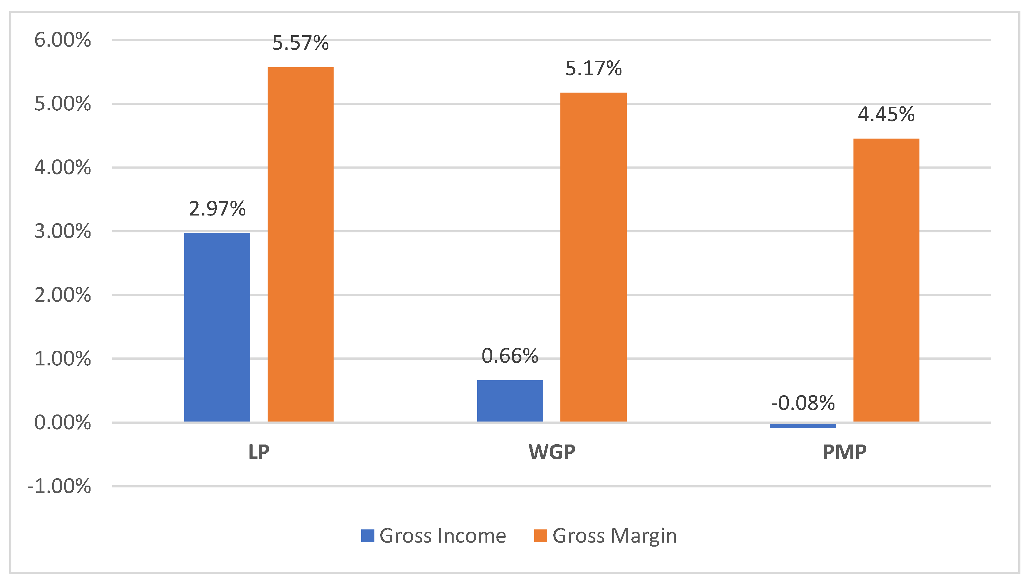
Figure 3 presents the percentage changes in the economic indicators (gross income and gross margin) after the application of the three mathematical models. Thus, there is an increase of 2.97% in the gross income in LP, but also a 0.66% increase in WGP, while the gross income decreases by −0.08% in PMP. Regarding the second economic indicator, in LP there is an increase of 5.57% while in WGP increases by 5.17% and in PMP model it increases by 4.45%.
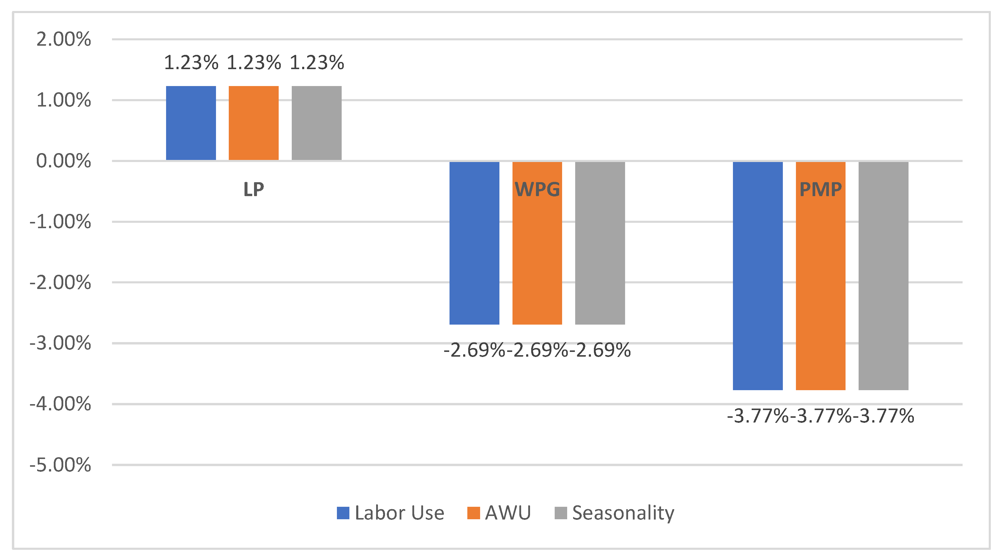
The percentage changes for the three social indicators (labor use, annual work units, and seasonality) are shown in Figure 4 below. There is an increase in labor use by 1.23%, in LP, while in WGP and in PMP it decreases by 2.69% and 3.77%, respectively. Annual work units showed an increase of 1.23% in LP, while in WGP and PMP it shows a decrease of 2.69% and 3.77%, respectively. Finally, seasonality increased in LP by 1.23% while it decreased by 2.69% in WGP and by 3.77% in the PMP model.
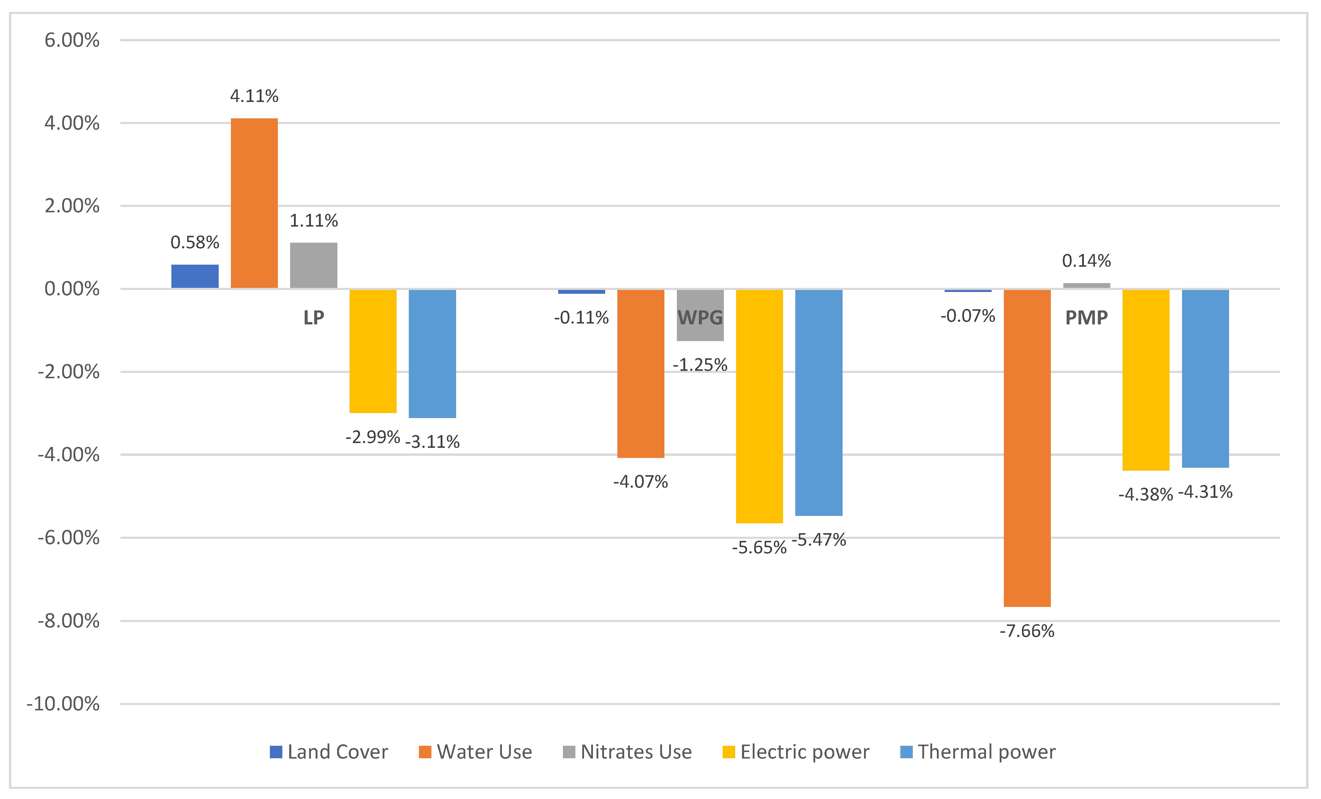
Finally, Figure 5 presents the percentage changes of the five environmental indicators, (land cover, water use, nitrate use, electric, and thermal power) after the application of the three mathematical models. The sixth environmental indicator (crop diversity) is not shown, since it is a number. In detail, the land cover shows an increase in the LP model at a rate of 0.58%, when it decreases in the WGP and PMP models by 0.11% and 0.07%, respectively. In water use, there is an increase in LP and a decrease in WGP and PMP models. However, an increase is also observed in the use of nitrates in the LP and PMP models, while a decrease is observed in the WGP model. The electric power is reduced during the implementation of the three mathematical programming models. A decrease is also observed in the thermal energy in all three models.
6. Discussion
The implementation of the three methodologies reorganized and optimized the real situations’ crop plan of the average farm of the sample. Subsequently, eleven economic, social, and environmental indicators derived from the literature review were calculated, both for the optimized crop plans and for the real situation crop plan. The real situation results of the selected indicators were compared to the results of the LP, WGP and PMP models.
Useful conclusions were drawn from the results of the implementation of the models. As for the LP model, it managed to achieve the highest increase in maximization of gross margin goals over the three models, as it was the main objective of the model. However, this increase also led to an increase in both fertilizer use and labor use, which were the farmers’ two other objectives. The PMP model achieved a gross margin increase at the lower level compared to the other two models. On the other hand, it met only one of the other two objectives, the minimization of labor use at a higher rate than the other two models, while fertilizer use remained almost constant. Regarding the participation of crops in the crop plans, the Positive Mathematical Programming model succeeded in reorganizing the average farm without abandoning a large number of the existing crops, which is one of the main advantages of using the method. On the other hand, the WGP method managed to achieve an increase in the gross margin of the farm, but not to the extent of that achieved by the LP method. At the same time, however, it was the only model that succeeded in achieving all the goals set by farmers.
As mentioned before, a comparison was also made regarding a set of 11 different indicators (economic, social, and environmental). The values for these indicators were calculated based on the results of the optimal crop plans of the three mathematical programming models.
The first economic indicator analyzed was gross income. Compared to the real situation of the average farm, an increase in gross income is observed in the optimal plans of the LP and WGP models, while a decrease in the crop plan of the PMP model was observed. This indicator shows the total income that the farm gains and cannot be a safe indicator of comparison between the models. Regarding the gross margin index resulting from the gross income after deducting the variable costs, the results showed that in all three mathematical programming models used, an increase in gross margin was observed compared to the real situation of the average farm. The rate of the increase corresponds to the model used.
The social indicators used were labor use, annual work units, and seasonality. Regarding the labor use, compared to the real situation an increase was observed with the application of the LP model, while on the contrary, with the application of the WGP and PMP models a decrease was observed. The indicator of annual work units moves at similar levels, which in the current situation is 1.55. In the LP model it increases, while in the WGP and PMP models it decreases. Finally, the seasonality of labor use also increases in the LP and decreases in the WGP and PMP models. Changes in social indicators are proportional to the total hours worked.
The six environmental indicators used were: crop diversity, land cover, water use, nitrates use, electric power production, and thermal power production from crop residues. The crop diversity in the real situation consists of 17 crops, while in LP and WGP decreased to 14; in the case of the PMP model it is 16, very close to the real situation. This result confirms that in the PMP the existing crops are reorganized without significant changes that can create problems for the farmer. The land cover in the real situation was equal to 74.84%. Greater land cover is shown by the crop plan proposed by the LP model with 75.28%, while smaller percentages of land coverage are shown by the production plans proposed by WGP with 74.77% and PMP models with 74.79%. Nevertheless, we observe that the crop plans of all three methods show land coverage close to 75%, with very small deviations. Regarding the water use indicator, it shows an increase in the LP model, while it shows a decrease in the WGP and PMP models. On the other hand, the indicator of nitrate use increases in the optimal crop plans of the LP and PMP models, while when applying the WGP model a decrease in nitrate use is observed. Electric power produced from crop residues is reduced in the optimal crop plan of all models. Finally, something similar happens in the last environmental indicator, thermal power production. Thermal power is reduced in the optimum crop plans proposed by all models, always compared to the real situation.
7. Conclusions
In this paper an attempt was made to compare mathematical programming methods that have been used widely in studies measuring the sustainability of farms. The selection of the appropriateness of these methods was confirmed by Arriaza and Gómez-Limón [57] who, in their study, compared the predictive performance of various mathematical models including Linear Programming, Positive Mathematical Programming, and Weighted Goal Programming. Finally, a short literature review of all three mathematical programming methods was carried out and then their mathematical forms were given. As mentioned before, the study area was the Region of Central Macedonia in Greece, and the sample was 219 beneficiaries who participated in measure ‘Modernization of agricultural holdings’.
We can summarize that the Linear Programming model managed to achieve the highest increase in gross margin over the PMP and WGP models but did not achieve the other two goal set by farmers. The use of the Linear Programming method is recommended in cases where we are interested in a single individual objective and for a specific growing season, since the LP model is considered static.
On the other hand, for the Positive Mathematical Programming model we can conclude that it manages to integrate dynamic elements into its objective function, since it can introduce changes in its various variables (costs, prices, subsidies, etc.) and calculates them automatically by entering the appropriate commands. For this reason, it can be easily adopted and used for different regions and types of farms. Its implementation succeeded in reorganizing the available factors of the average farm without abandoning a large part of the existing crops, which is one of the main advantages of using the method. Its use is indicated in cases where we are interested in reorganization of the crop plan without major changes from the existing plan. Although the model is basically considered static, it can be transformed into a dynamic one by using longitudinal data, mainly to incorporate risk into the objective function, as well as to simulate various scenarios.
Finally, the WGP managed to achieve an increase in the gross margin of the farm, but not to the level achieved by the LP model; but at the same time, it was the only model that achieved a reduction in both the fertilizer use and the labor use, which were the other two goals set by farmers.The WGP model can be used in cases where we are interested in achieving more than one goal, since it achieves the integration of separate conflicting goals into one utility function.
Funding
This research received no external funding.
Institutional Review Board Statement
Not applicable.
Informed Consent Statement
Not applicable.
Data Availability Statement
Not applicable.
Conflicts of Interest
The author declares no conflict of interest.
References
- Bournaris, T.; Moulogianni, C.; Vlontzos, G.; Georgilas, I. Methodologies Used to Assess the Impacts of Climate Change in Agricultural Economics: A Rapid Review. Int. J. Sustain. Agric. Manag. Informatics 2021, 7, 253–269. [Google Scholar] [CrossRef]
- Ewert, F.; van Ittersum, M.K.; Heckelei, T.; Therond, O.; Bezlepkina, I.V.; Andersen, E. Scale Changes and Model Linking Methods for Integrated Assessment of Agri-Environmental Systems. Agric. Ecosyst. Environ. 2011, 142, 6–17. [Google Scholar] [CrossRef]
- Reidsma, P.; Wolf, J.; Kanellopoulos, A.; Schaap, B.F.; Mandryk, M.; Verhagen, J.; Van Ittersum, M.K. Climate Change Impact and Adaptation Research Requires Integrated Assessment and Farming Systems Analysis: A Case Study in the Netherlands. Environ. Res. Lett. 2015, 10, 045004. [Google Scholar] [CrossRef]
- Angulo, C.; Rötter, R.; Lock, R.; Enders, A.; Fronzek, S.; Ewert, F. Implication of Crop Model Calibration Strategies for Assessing Regional Impacts of Climate Change in Europe. Agric. For. Meteorol. 2013, 170, 32–46. [Google Scholar] [CrossRef]
- Bournaris, T.; Vlontzos, G.; Moulogianni, C. Efficiency of Vegetables Produced in Glasshouses: The Impact of Data Envelopment Analysis (DEA) in Land Management Decision Making. Land 2019, 8, 17. [Google Scholar] [CrossRef]
- Arfini, F. Mathematical Programming Models Employed in the Analysis of the Common Agriculture Policy; National Institute of Agricultural Economics, INEA: Roma, Italy, 2001. [Google Scholar]
- Buysse, J.; Van Huylenbroeck, G.; Lauwers, L. Normative, Positive and Econometric Mathematical Programming as Tools for Incorporation of Multifunctionality in Agricultural Policy Modelling. Agric. Ecosyst. Environ. 2007, 120, 70–81. [Google Scholar] [CrossRef]
- Paas, W.; Kanellopoulos, A.; van de Ven, G.; Reidsma, P. Integrated Impact Assessment of Climate and Socio-Economic Change on Dairy Farms in a Watershed in the Netherlands. NJAS Wagening. J. Life Sci. 2016, 78, 35–45. [Google Scholar] [CrossRef]
- Challinor, A.J.; Watson, J.; Lobell, D.B.; Howden, S.M.; Smith, D.R.; Chhetri, N. A Meta-Analysis of Crop Yield under Climate Change and Adaptation. Nat. Clim. Chang. 2014, 4, 287–291. [Google Scholar] [CrossRef]
- Lobell, D.B.; Burke, M.B. On the Use of Statistical Models to Predict Crop Yield Responses to Climate Change. Agric. For. Meteorol. 2010, 150, 1443–1452. [Google Scholar] [CrossRef]
- Rötter, R.P.; Carter, T.R.; Olesen, J.E.; Porter, J.R. Crop–Climate Models Need an Overhaul. Nat. Clim. Chang. 2011, 1, 175–177. [Google Scholar] [CrossRef]
- Zagaria, C.; Schulp, C.J.E.; Zavalloni, M.; Viaggi, D.; Verburg, P.H. Modelling Transformational Adaptation to Climate Change among Crop Farming Systems in Romagna, Italy. Agric. Syst. 2021, 188, 103024. [Google Scholar] [CrossRef]
- Berbel, J.; Expósito, A. A Decision Model for Stochastic Optimization of Seasonal Irrigation-Water Allocation. Agric. Water Manag. 2022, 262, 107419. [Google Scholar] [CrossRef]
- Markou, M.; Michailidis, A.; Loizou, E.; Nastis, S.A.; Lazaridou, D.; Kountios, G.; Allahyari, M.S.; Stylianou, A.; Papadavid, G.; Mattas, K. Applying a Delphi-Type Approach to Estimate the Adaptation Cost on Agriculture to Climate Change in Cyprus. Atmosphere 2020, 11, 536. [Google Scholar] [CrossRef]
- Schönhart, M.; Schauppenlehner, T.; Schmid, E.; Muhar, A. Integration of Bio-Physical and Economic Models to Analyze Management Intensity and Landscape Structure Effects at Farm and Landscape Level. Agric. Syst. 2011, 104, 122–134. [Google Scholar] [CrossRef]
- Chatzinikolaou, P.; Viaggi, D.; Raggi, M. Review of Multicriteria Methodologies and Tools for the Evaluation of the Provision of Ecosystem Services; Springer: Cham, Switzerland, 2018; pp. 43–68. [Google Scholar] [CrossRef]
- Audsley, E.; Trnka, M.; Sabaté, S.; Maspons, J.; Sanchez, A.; Sandars, D.; Balek, J.; Pearn, K. Interactively Modelling Land Profitability to Estimate European Agricultural and Forest Land Use under Future Scenarios of Climate, Socio-Economics and Adaptation. Clim. Chang. 2014, 128, 215–227. [Google Scholar] [CrossRef]
- Jäger, J.; Rounsevell, M.D.A.; Harrison, P.A.; Omann, I.; Dunford, R.; Kammerlander, M.; Pataki, G. Assessing Policy Robustness of Climate Change Adaptation Measures across Sectors and Scenarios. Clim. Chang. 2014, 128, 395–407. [Google Scholar] [CrossRef]
- Topp, C.F.E.; Mitchell, M. Forecasting the Environmental and Socio-Economic Consequences of Changes in the Common Agricultural Policy. Agric. Syst. 2003, 76, 227–252. [Google Scholar] [CrossRef]
- Berbel, J.; Martínez-Dalmau, J. A Simple Agro-Economic Model for Optimal Farm Nitrogen Application under Yield Uncertainty. Agronomy 2021, 11, 1107. [Google Scholar] [CrossRef]
- Bell, S.; Morse, S. Sustainability Indicators: Measuring the Immeasurable? Routledge: London, UK, 2008. [Google Scholar]
- Pinar, M.; Cruciani, C.; Giove, S.; Sostero, M. Constructing the FEEM Sustainability Index: A Choquet Integral Application. Ecol. Indic. 2014, 39, 189–202. [Google Scholar] [CrossRef]
- Chatzinikolaou, P.; Bournaris, T.; Kiomourtzi, F.; Moulogianni, C.; Manos, B. Classification and Ranking Rural Areas in Greece Based on Technical, Economic and Social Indicators of the Agricultural Holdings. Int. J. Bus. Innov. Res. 2015, 9, 455–469. [Google Scholar] [CrossRef]
- Manos, B.; Bournaris, T.; Moulogianni, C.; Kiomourtzi, F. Assessment of Rural Development Plan Measures in Greece. Int. J. Oper. Res. 2017, 28, 448–471. [Google Scholar] [CrossRef]
- Moulogianni, C.; Bournaris, T.; Manos, B.; Nastis, S. Farm Planning in Nitrate Sensitive Agricultural Areas. Int. J. Environ. Sustain. Dev. 2012, 11, 105–117. [Google Scholar] [CrossRef]
- Moulogianni, C.; Bournaris, T.; Manos, B. A Bilevel Programming Model for Farm Planning in Nitrates Sensitive Agricultural Areas. New Medit 2011, 10, 41. [Google Scholar]
- Gómez-Limón, J.A.; Sanchez-Fernandez, G. Empirical Evaluation of Agricultural Sustainability Using Composite Indicators. Ecol. Econ. 2010, 69, 1062–1075. [Google Scholar] [CrossRef]
- Dantsis, T.; Douma, C.; Giourga, C.; Loumou, A.; Polychronaki, E.A. A Methodological Approach to Assess and Compare the Sustainability Level of Agricultural Plant Production Systems. Ecol. Indic. 2010, 10, 256–263. [Google Scholar] [CrossRef]
- Ribeiro Gonçalves, J.R.M.; Araújo E Silva Ferraz, G.; Reynaldo, É.F.; Marin, D.B.; Ferraz, P.F.P.; Pérez-Ruiz, M.; Rossi, G.; Vieri, M.; Sarri, D. Comparative Analysis of Soil-Sampling Methods Used in Precision Agriculture. J. Agric. Eng. 2021, 52. [Google Scholar] [CrossRef]
- Bradley, S.P.; Hax, A.C.; Magnanti, T.L. Applied Mathematical Programming; Addison-Wesley: Boston, MA, USA, 1977; p. 539. [Google Scholar]
- Alotaibi, A.; Nadeem, F. A Review of Applications of Linear Programming to Optimize Agricultural Solutions. Int. J. Inf. Eng. Electron. Bus. 2021, 13, 11–21. [Google Scholar] [CrossRef]
- Manos, B.; Papanagiotou, E. Fruit-Tree Replacement in Discrete Time: An Application in Central Macedonia. Eur. Rev. Agric. Econ. 1983, 10, 69–78. [Google Scholar] [CrossRef]
- Manos, B.; Kitsopanidis, G. Mathematical Programming Models for Farm Planning. Oxf. Agrar. Stud. 2007, 17, 163–172. [Google Scholar] [CrossRef]
- Rozakis, S.; Tsiboukas, K.; Petsakos, A. Greek Cotton Farmers’ Supply Response to Partial Decoupling of Subsidies. In Proceedings of the 2008 International Congress, Ghent, Belgium, 26–29 August 2008. [Google Scholar] [CrossRef]
- Moulogianni, C.; Bournaris, T.; Reeves, M.; Maher, A.T. Assessing the Impacts of Rural Development Plan Measures on the Sustainability of Agricultural Holdings Using a PMP Model. Land 2021, 10, 446. [Google Scholar] [CrossRef]
- Gohin, A.; Chantreuil, F. La Programmation Mathématique Positive Dans Les Modèles d’exploitation Agricole. Principes et Importance Du Calibrage. Rev. d’Études en Agric. Environ. 1999, 52, 59–78. [Google Scholar] [CrossRef]
- Heckelei, T.; Britz, W.; Zhang, Y. Positive Mathematical Programming Approaches—Recent Developments in Literature and Applied Modelling. Bio-Based Appl. Econ. 2012, 1, 109–124. [Google Scholar] [CrossRef]
- Röhm, O.; Dabbert, S. Integrating Agri-Environmental Programs into Regional Production Models: An Extension of Positive Mathematical Programming. Am. J. Agric. Econ. 2003, 85, 254–265. [Google Scholar] [CrossRef]
- Petsakos, A.; Rozakis, S. Integrating Risk and Uncertainty in PMP Models. In Proceedings of the 2011 International Congress of European Association of Agricultural Economists, Zurich, Switzerland, 30 August–2 September 2011. [Google Scholar]
- Petsakos, A.; Rozakis, S. Critical Review and State-of-the-Art of PMP Models: An Application to Greek Arable Agriculture. Res. Top. Agric. Appl. Econ. 2012, 1, 36–63. [Google Scholar] [CrossRef]
- Kanellopoulos, A.; Berentsen, P.; Heckelei, T.; Van Ittersum, M.; Lansink, A.O. Assessing the Forecasting Performance of a Generic Bio-Economic Farm Model Calibrated with Two Different PMP Variants. J. Agric. Econ. 2010, 61, 274–294. [Google Scholar] [CrossRef]
- Janssen, S.; Louhichi, K.; Kanellopoulos, A.; Zander, P.; Flichman, G.; Hengsdijk, H.; Meuter, E.; Andersen, E.; Belhouchette, H.; Blanco, M.; et al. A Generic Bio-Economic Farm Model for Environmental and Economic Assessment of Agricultural Systems. Environ. Manag. 2010, 46, 862–877. [Google Scholar] [CrossRef]
- Louhichi, K.; Kanellopoulos, A.; Janssen, S.; Flichman, G.; Blanco, M.; Hengsdijk, H.; Heckelei, T.; Berentsen, P.; Lansink, A.O.; Ittersum, M. Van FSSIM, a Bio-Economic Farm Model for Simulating the Response of EU Farming Systems to Agricultural and Environmental Policies. Agric. Syst. 2010, 103, 585–597. [Google Scholar] [CrossRef]
- Barkaoui, A.; Butault, J.-P. Cereals and Oilseeds Supply within the EU, under AGENDA 2000: A Positive Mathematical Programming Application. Agric. Econ. Rev. 2000, 1, 1–12. [Google Scholar] [CrossRef]
- Cypris, C. Positive Mathematische Programmierung (PMP) im Agrarsektormodell RAUMIS. In Schriftenreihe der Forschungsgesellschaft für Agrarpolitik und Agrarsoziologie; FAA: Bonn, Germany, 2000; ISBN 3884883135. [Google Scholar]
- Fragoso, R.M.; Carvalho, M.L.d.S.; Henriques, P.D.d.S. Positive Mathematical Programming: A Comparison of Different Specification Rules. In Proceedings of the Congress of the European Association of Agricultural Economists, Ghent, Belgium, 26–29 August 2008. [Google Scholar] [CrossRef]
- Arfini, F.; Donati, M.; Marongiu, S.; Cesaro, L. Farm Production Costs Estimation Trough PMP Models: An. Application in Three Italian Regions. In Proceedings of the 2012 First Congress, Trento, Italy, 4–5 June 2012. [Google Scholar]
- Howitt, R.E.; Medellín-Azuara, J.; MacEwan, D.; Lund, J.R. Calibrating Disaggregate Economic Models of Agricultural Production and Water Management. Environ. Model. Softw. 2012, 38, 244–258. [Google Scholar] [CrossRef]
- Prišenk, J.; Turk, J.; Rozman, Č.; Borec, A.; Zrakić, M.; Pažek, K. Advantages of Combining Linear Programming and Weighted Goal Programming for Agriculture Application. Oper. Res. 2014, 14, 253–260. [Google Scholar] [CrossRef]
- Bournaris, T.; Moulogianni, C.; Manos, B. A Multicriteria Model for the Assessment of Rural Development Plans in Greece. Land Use Policy 2014, 38, 1–8. [Google Scholar] [CrossRef]
- Manos, B.; Bournaris, T.; Papathanasiou, J.; Chatzinikolaou, P. Tobacco Decoupling Impacts on Income, Employment and Environment in European Tobacco Regions. Int. J. Bus. Innov. Res. 2010, 4, 281–297. [Google Scholar] [CrossRef]
- Manos, B.; Bournaris, T.; Kamruzzaman, M.; Begum, M.; Anjuman, A.; Papathanasiou, J. Regional Impact of Irrigation Water Pricing in Greece under Alternative Scenarios of European Policy: A Multicriteria Analysis. Reg. Stud. 2006, 40, 1055–1068. [Google Scholar] [CrossRef]
- Bournaris, T.; Papathanasiou, J.; Moulogianni, C.; Manos, B. A Fuzzy Multicriteria Mathematical Programming Model for Planning Agricultural Regions. New Medit 2009, 8, 22–27. [Google Scholar]
- Manos, B.; Papathanasiou, J.; Bournaris, T.; Paparrizou, A.; Arabatzis, G. Simulation of Impacts of Irrigated Agriculture on Income, Employment and Environment. Oper. Res. 2009, 9, 251–266. [Google Scholar] [CrossRef]
- Manos, B.; Papathanasiou, J.; Bournaris, T.; Voudouris, K. A Multicriteria Model for Planning Agricultural Regions within a Context of Groundwater Rational Management. J. Environ. Manag. 2010, 91, 1593–1600. [Google Scholar] [CrossRef]
- Recchia, L.; Boncinelli, P.; Cini, E.; Vieri, M.; Pegna, F.G.; Sarri, D. Multicriteria Analysis and LCA Techniques: With Applications to Agro-Engineering Problems. In Green Energy and Technology; Springer: London, UK, 2011; Volume 91. [Google Scholar] [CrossRef]
- Arriaza, M.; Gómez-Limón, J.A. Comparative Performance of Selected Mathematical Programming Models. Agric. Syst. 2003, 77, 155–171. [Google Scholar] [CrossRef]
- Howitt, R.E. Positive Mathematical Programming. Am. J. Agric. Econ. 1995, 77, 329–342. [Google Scholar] [CrossRef]
- Heckelei, T. Estimation of Constrained Optimisation Models for Agricultural Supply Analysis Based on Generalised Maximum Entropy. Eur. Rev. Agric. Econ. 2003, 30, 27–50. [Google Scholar] [CrossRef]
- Sumpsi, J.M.; Amador, F.; Romero, C. On Farmers’ Objectives: A Multi-Criteria Approach. Eur. J. Oper. Res. 1997, 96, 64–71. [Google Scholar] [CrossRef]
- Amador, F.; Sumpsi, J.M.; Romero, C. A Non-Interactive Methodology to Assess Farmers’ Utility Functions: An Application to Large Farms in Andalusia, Spain. Eur. Rev. Agric. Econ. 1998, 25, 92–102. [Google Scholar] [CrossRef]
- Romero, C. Handbook of Critical Issues in Goal Programming; Pergamon Press: Oxford, UK, 1991; ISBN 9780080406619. [Google Scholar]
- Georgilas, I.; Moulogianni, C.; Bournaris, T.; Vlontzos, G.; Manos, B. Socioeconomic Impact of Climate Change in Rural Areas of Greece Using a Multicriteria Decision-Making Model. Agronomy 2021, 11, 1779. [Google Scholar] [CrossRef]
- Chatzinikolaou, P.; Bournaris, T.; Manos, B. Multicriteria Analysis for Grouping and Ranking European Union Rural Areas Based on Social Sustainability Indicators. Int. J. Sustain. Dev. 2013, 16, 335. [Google Scholar] [CrossRef]
Figure 1.
The region of Central Macedonia. Source: Wikipedia.

Figure 2.
Real Situation Crop Plan for the average farm. Source: Hellenic Statistical Authority.

Figure 3.
Changes in the economic indicators. Source: Our elaboration.

Figure 4.
Changes in Social Indicators. Source: Our elaboration.

Figure 5.
Changes in Environmental Indicators. Source: Our elaboration.


Table 1.
Selected Economic, Social and Environmental Indicators.
| Indicators | Units | |
|---|---|---|
| Economic | Gross Income | EUR |
| Gross Margin | EUR | |
| Social | Labor Use | hours |
| Annual Work Units | AWU | |
| Seasonality | hours/month | |
| Environmental | Crop diversity | Number of crops |
| Land Cover | % | |
| Water Use | m3 | |
| Nitrates Use | kg | |
| Electric power | MWh | |
| Thermal power | MWh |
Table 2.
Comparison of the Real crop plan vs. LP crop plan. Source: Our elaboration.
| Real | LP | ||
|---|---|---|---|
| Values | % Deviation | ||
| Gross Margin (EUR) | 15,699 | 16,573 | 5.6 |
| Fertilizers use (kg) | 6791 | 6867 | 1.1 |
| Labor Use (hours) | 2715 | 2748 | 1.2 |
| Cotton | 10.80 | 5.72 | −47.0 |
| Common wheat | 5.03 | 0.00 | −100.0 |
| Durum wheat | 27.79 | 33.29 | 19.8 |
| Sugarbeets | 2.45 | 0.00 | −100.0 |
| Barley | 5.15 | 6.70 | 30.0 |
| Alfalfa | 7.29 | 8.74 | 20.0 |
| Maize | 8.97 | 10.76 | 19.9 |
| Olive trees | 1.84 | 1.93 | 4.7 |
| Rice | 16.72 | 20.07 | 20.0 |
| Sunflower | 1.46 | 1.89 | 29.9 |
| Tomatoes | 0.92 | 1.10 | 19.8 |
| Potatoes | 0.55 | 0.67 | 20.8 |
| Cherry trees | 5.45 | 5.72 | 4.9 |
| Apple trees | 0.85 | 0.90 | 5.4 |
| Peach trees | 2.05 | 2.15 | 4.8 |
| Kiwi | 0.34 | 0.36 | 4.9 |
| Vetch | 2.33 | 0.00 | −100.0 |
| Total | 100.0 | 100.0 | |
Table 3.
Comparison of the Real crop plan vs. PMP model crop plan. Source: Our elaboration.
| Real | PMP | ||
|---|---|---|---|
| Values | % Deviation | ||
| Gross Margin (EUR) | 15,699 | 16,398 | 4.5 |
| Fertilizers use (kg) | 6791 | 6801 | 0.1 |
| Labor Use (hours) | 2715 | 2613 | −3.8 |
| Cotton | 10.80 | 4.00 | −62.9 |
| Common wheat | 5.03 | 4.96 | −1.5 |
| Durum wheat | 27.79 | 32.48 | 16.9 |
| Sugarbeets | 2.45 | 0.00 | −100.0 |
| Barley | 5.15 | 6.12 | 18.7 |
| Alfalfa | 7.29 | 8.74 | 20.0 |
| Maize | 8.97 | 10.76 | 19.9 |
| Olive trees | 1.84 | 1.93 | 4.7 |
| Rice | 16.72 | 16.55 | −1.0 |
| Sunflower | 1.46 | 1.45 | −0.4 |
| Tomatoes | 0.92 | 0.92 | −0.2 |
| Potatoes | 0.55 | 0.67 | 20.8 |
| Cherry trees | 5.45 | 5.72 | 4.9 |
| Apple trees | 0.85 | 0.90 | 5.4 |
| Peach trees | 2.05 | 2.15 | 4.8 |
| Kiwi | 0.34 | 0.36 | 4.9 |
| Vetch | 2.33 | 2.30 | −1.3 |
| Total | 100.0 | 100.0 | |
Table 4.
Comparison of the Real situation crop plan vs. WGP model optimum crop plan. Source: Our elaboration.
Table 4.
Comparison of the Real situation crop plan vs. WGP model optimum crop plan. Source: Our elaboration.
| Real | WGP | ||
|---|---|---|---|
| Values | % Deviation | ||
| Gross Margin (EUR) | 15,699 | 16,511 | 5.2 |
| Fertilizers use (kg) | 6791 | 6706 | −1.3 |
| Labor Use (hours) | 2715 | 2642 | −2.7 |
| Cotton | 10.80 | 0.00 | −100.0 |
| Common wheat | 5.03 | 0.00 | −100.0 |
| Durum wheat | 27.79 | 35.98 | 29.5 |
| Sugarbeets | 2.45 | 0.00 | −100.0 |
| Barley | 5.15 | 6.70 | 30.0 |
| Alfalfa | 7.29 | 8.74 | 20.0 |
| Maize | 8.97 | 10.76 | 19.9 |
| Olive trees | 1.84 | 1.93 | 4.7 |
| Rice | 16.72 | 20.07 | 20.0 |
| Sunflower | 1.46 | 1.89 | 29.9 |
| Tomatoes | 0.92 | 1.10 | 19.8 |
| Potatoes | 0.55 | 0.67 | 20.8 |
| Cherry trees | 5.45 | 5.72 | 4.9 |
| Apple trees | 0.85 | 0.90 | 5.4 |
| Peach trees | 2.05 | 2.15 | 4.8 |
| Kiwi | 0.34 | 0.36 | 4.9 |
| Vetch | 2.33 | 3.03 | 30.2 |
| Total | 100.0 | 100.0 | |
Table 5.
Comparison of mathematical programming models for the sustainability indicators. Source: Our elaboration.
Table 5.
Comparison of mathematical programming models for the sustainability indicators. Source: Our elaboration.
| Real | PMP | LP | WGP | ||||
|---|---|---|---|---|---|---|---|
| Values | Values | % Deviation | Values | % Deviation | Values | % Deviation | |
| Economic | |||||||
| Gross Margin (EUR) | 15,699 | 16,398 | 4.45% | 16,573 | 5.57% | 16,511 | 5.17% |
| Gross Income (EUR) | 29,499 | 29,475 | −0.08% | 30,375 | 2.97% | 29,694 | 0.66% |
| Social | |||||||
| Labor Use (hours) | 2715 | 2.613 | −3.77% | 2748 | 1.23% | 2642 | −2.69% |
| Annual Work Units (AWU) | 1.55 | 1.49 | −3.77% | 1.57 | 1.23% | 1.51 | −2.69% |
| Seasonality (hours/month) | 226.24 | 217.73 | −3.77% | 229.03 | 1.23% | 220.17 | −2.69% |
| Environmental | |||||||
| Crop Diversity (number) | 17 | 16 | −5.88% | 14 | −17.65% | 14 | −17.65% |
| Land Cover (%) | 74.84 | 74.79 | −0.07% | 75.28 | 0.58% | 74.77 | −0.11% |
| Water Use (m3) | 38,435 | 35,491 | −7.66% | 40,016 | 4.11% | 36,870 | −4.07% |
| Nitrates Use (kg) | 6791 | 6801 | 0.14% | 6867 | 1.11% | 6706 | −1.25% |
| Electric power (MWh) | 21.46 | 20.52 | −4.38% | 20.82 | −2.99% | 20.25 | −5.65% |
| Thermal power (MWh) | 97.04 | 92.85 | −4.31% | 94.02 | −3.11% | 91.73 | −5.47% |
Publisher’s Note: MDPI stays neutral with regard to jurisdictional claims in published maps and institutional affiliations. |
© 2022 by the author. Licensee MDPI, Basel, Switzerland. This article is an open access article distributed under the terms and conditions of the Creative Commons Attribution (CC BY) license (https://creativecommons.org/licenses/by/4.0/).
Share and Cite
MDPI and ACS Style
Moulogianni, C. Comparison of Selected Mathematical Programming Models Used for Sustainable Land and Farm Management. Land 2022, 11, 1293. https://doi.org/10.3390/land11081293
AMA Style
Moulogianni C. Comparison of Selected Mathematical Programming Models Used for Sustainable Land and Farm Management. Land. 2022; 11(8):1293. https://doi.org/10.3390/land11081293
Chicago/Turabian StyleMoulogianni, Christina. 2022. "Comparison of Selected Mathematical Programming Models Used for Sustainable Land and Farm Management" Land 11, no. 8: 1293. https://doi.org/10.3390/land11081293
Note that from the first issue of 2016, this journal uses article numbers instead of page numbers. See further details here.