Simulation Analysis of Land-Use Pattern Evolution and Valuation of Terrestrial Ecosystem Carbon Storage of Changzhi City, China

Abstract

Carbon sequestration in terrestrial ecosystems is critical for combating global climate change and achieving regional carbon neutrality, and LUCC is a vital factor influencing the carbon cycle process of terrestrial ecosystems and causing changes in carbon sources/sinks. This study analyzes the drivers of LUCC based on a review of the dynamics of LUCC in Changzhi from 2000 to 2020, analyzes the driving factors of LUCC using the Clue-S model and binary logistic regression analysis model, then simulates land-use patterns under different scenarios in 2030 by the CA-Markov model, and finally analyzes carbon stock changes and spatial distribution characteristics in different periods from the perspective of carbon source/sink interconversion with the help of InVEST model. The results show: (1) in the past two decades, more than 90% of the expansion of artificial surfaces in Changzhi comes from cultivated land. Ecological conservation policies are more decisive in influencing LUCC than natural, social, and transportation accessibility factors. (2) During the 20 years, the total carbon stock increased by 680,989.73 t, with the carbon emission control area accounting for 7.5%, mainly distributed near urban centers and coal mining areas. The carbon sink enhancement area accounts for 5.5% and is mainly concentrated near forest land and ecological and nature reserves. (3) The spatial location of cities influences the density of carbon stock in the adjacent range. Carbon stock density increases within the buffer zone with the distance from urban center, county center, expressways, national highway, settlements, rivers, provincial roads, reservoirs, railways, county highway, and village roads. The rate of carbon stock increase per 100 m is 0.12 t/ha, 0.25 t/ha, 0.17 t/ha, 0.36 t/ha, 0.71 t/ha, 0.33 t/ha, 0.38 t/ha, 0.57 t/ha, 0.23 t/ha, 0.46 t/ha, and 0.48 t/ha respectively. The higher the administrative center and road grades, the lower the carbon density will be instead. (4) In the 2030 CD scenario, compared with the ND scenario, the cultivated land and grassland are effectively protected and the cultivated land area is increased by 445.68 km², while the expansion of artificial surface is suppressed and the area is reduced by 448.2 km², which ultimately leads to a reduction in carbon loss of 392,011.85 t. Future ecological management should focus on protecting high-value carbon sink areas and carbon sink enhancement areas and the ecological management and restoration of low-value carbon sink areas and carbon emission control areas.

1. Introduction

The environmental difficulties caused by rising CO₂ levels have sparked widespread concern worldwide. Thus it is critical to look into measures to minimize carbon emissions and improve carbon sequestration capability in the context of carbon peaking and carbon neutrality [1,2]. Over the last few decades, terrestrial ecosystems have played a critical role in mitigating the greenhouse effect and regulating regional climate by acting as an essential component of the global carbon pool, absorbing about 3 Pg C from the atmosphere each year, which is about one-third of total CO₂ emissions [3,4]. The capacity of different ecosystems to capture carbon varies, and within the same type of ecosystem, there is temporal and spatial heterogeneity in the distribution of carbon stocks [5,6]. LUCC plays a significant role in global carbon emissions as a substantial element impacting the carbon cycle process of terrestrial ecosystems and causing changes in carbon sources/sinks. Over the last decade (2010–2019), global average yearly CO₂ emissions have been 9.4 ± 0.5 GT C, with LUCC accounting for 14% (1 t of carbon, when completely burned in oxygen, produces approximately 3.67 (=44/12) t of CO₂. The amount of CO₂ and the amount of carbon emissions (C) are convertible, that is, fixing 1 t of carbon is equivalent to absorbing 3.67 t of CO₂). Therefore, accurate and scientific simulations of land-use changes are the foundation for analyzing regional carbon stock changes and solving ecological and environmental problems. They can provide a reference for the formulation of regional land planning and ecological environment management [7]. Land-use change studies are further divided into proximate cause studies, which refer to human activities or direct behaviors, and potential drivers, which refer to the socio-economic and biophysical environmental processes that drive these proximate causes [8]. The foundation for LUCC simulations is a deep understanding of the driving mechanisms of land-use change [9]. The combined implementation of the International Human Dimensions Programme on Global Environmental Change (IHDP) and the International Geosphere-Biosphere Programme (IGBP) has significantly contributed to the advancement of LUCC science and associated research over the past 20 years [10]. Carrying out systematic and diversified land-use scenario simulations based on land-use prediction models can help people understand the mechanisms of social, economic, and physical variables and land-use change response more directly. Such models are the system dynamics model, artificial neural networks model, stochastic prediction model, empirical regression model, cellular automata (CA)-Markov model, and land-use conversion and its effects (CLUE)-S model [11,12,13]. In comparison to the limitations of other models, such as the Clue-S model and the System Dynamics model, suitable for small urban areas [14,15], the CA-Markov model has a much grander scale and domain of applicability. The model combines the CA model’s ability to simulate spatial changes in complex systems with the Markov model’s ability to predict long-term changes in land-use patterns, which not only improves the prediction accuracy of land-use type transformation but also effectively simulates spatial changes in land-use patterns, which is both scientific and practical [16,17].

Methods for assessing the carbon stocks of regional terrestrial ecosystems fall into roughly two categories: “bottom-up” and “top-down.” Inventory methods and eddy covariance methods are two common “bottom-up” methods based on the results of sample site surveys and extended to the whole region; atmospheric inversions, which invert terrestrial ecosystem carbon sink based on atmospheric CO₂ concentrations, are examples of “top-down” methods [18]. The inventory method, which primarily includes the accumulation and biomass methods, is easy to operate and practical. However, they are based on intensive field surveys. The entire process is time-consuming, labor-intensive, costly, and time-consuming, and the spatial heterogeneity of terrestrial ecosystems can affect experimental results. [19,20]. Based on meteorological principles, eddy covariance can directly measure the net CO₂ exchange between regional inland ecosystems and the atmosphere [21], but expensive, representative errors in field measurements and the inability to distinguish between soil carbon budget and above-ground and below-ground biomass remain an unavoidable practical problem [22]. The atmospheric inversion method estimates terrestrial carbon sinks using the atmospheric transport model and CO₂ molar fractions. Its main advantage is monitoring regional terrestrial carbon sinks’ reactions to climate change in real-time [23]. The limitation is that the accuracy of the current atmospheric inversion is greatly affected by the number and distribution of observation points, and the spatial resolution of the obtained carbon flux data results is so low that the carbon fluxes of each ecosystem type cannot be accurately subdivided. Moreover, these methods are difficult to accurately reflect the response of carbon stock changes to natural and human activities on a large scale and over a long-time continuum. Based on this, a model-based approach to carbon stock assessment has emerged. Previous research has demonstrated that the INVEST model is a reliable and straightforward estimating method for carbon stock assessment at various spatial scales, with low data needs, easy access, and speedy operation. A thorough, dynamic, and visual assessment of ecosystem carbon storage functions can be made at various global, national, and regional dimensions [24]. The InVEST model can dramatically reduce financial expenses and enable dynamic quantification of ecosystem service value, making it more practical than prior ecosystem service valuation methods, which were static and monolithic. It is currently widely utilized in many countries and regions. Furthermore, the study region’s physical, geographic, and socio-economic data can be input into the investment model to derive trends in ecosystem carbon storage’s spatial distribution and evolution under current or potential future scenarios. Through scenario modification, investment models may also quantify human activities’ positive and negative effects on ecosystem carbon storage, offering a scientific foundation for resolving local, regional, and even global resource and environmental issues [25].

In recent years, many scholars have studied the carbon stocks of some or overall terrestrial ecosystems based on changes in land-use patterns. Fernandes et al. used the CA-Markov and InVEST models to simulate carbon stock changes in the Sergipe semiarid region, Brazil, in 2030 under a variety of scenarios, showing that the conservation scenario contributes to the recovery of carbon sequestration [26]. Zhang Yan et al. used the Clue-S model and InVEST model to simulate the land-use pattern of the Fen River basin in Shanxi, China under multiple scenarios, and the results showed that under the natural growth scenario in 2030, the carbon stock and carbon intensity of the upper Fen River would decline significantly, by 176,917.5 t compared to 2017. While the ecological conservation scenario could change this trend, the ecological protection scenario can also change this trend, resulting in a significant increase in carbon stock and carbon intensity, reaching 2,164,299.18 t and 0.41 t/ha, respectively [27]. In the context of carbon neutrality and carbon peaking, changes in carbon stocks in coal-energy-related terrestrial ecosystems in resource-based cities are of greater concern. In recent decades, China’s rapid economic development has been accompanied by an increase in energy demand, with coal accounting for 56.8% of the country’s total energy consumption in 2020. For some time to come, coal will continue to be China’s main energy source. Large-scale mining of coal resources has caused massive damage to the land surface and affected pristine ecosystem functions, including carbon storage functions [28]. Most existing studies have mostly surveyed carbon stocks based on what exists within mines, without comparing land-use changes within the mine boundaries with the surrounding area to highlight the differences. For example, Huping Hou et al. found that carbon stocks and carbon density in the study area decreased by 16,049.45 t and 69.87 g m⁻², respectively, between 1987 and 2008, using remote sensing data [29]. The land-use pattern changes in the study area are not contrasted with the surrounding land-use changes. Furthermore, land-use pattern change is a dynamic process and existing studies do not analyze and estimate future changes in carbon stocks in terrestrial ecosystems, nor do these studies explain the contribution of land reclamation to increasing carbon stocks, and land reclamation and restoration are considered to be key to mitigating or reversing these effects. Therefore, studying the spatial and temporal effects of regional land-use pattern change on carbon stocks within terrestrial ecosystems could provide land restoration and reclamation that can provide valuable information that can contribute to regional ecological development and promote optimal allocation of land use. Based on this, this research conducts a multi-scenario land-use change simulation based on land-use change in Changzhi City to analyze the changes in terrestrial ecosystem carbon stocks and their spatial distribution patterns. Not only does this provide guidance and data support for future land-use structure optimization and terrestrial ecosystem carbon sink investigations, but it also has significant implications for regional sustainable development and climate change mitigation. This study intends to: (1) review the dynamic changes in LUCC in Changzhi from 2000 to 2020, analyze the driving forces of LUCC, and divide the carbon sink function area based on regional carbon stock calculations; (2) based on the results of carbon storage in Changzhi in 2020, perform spatial pattern analysis to calculate and analyze the average carbon stock density at various distances near urban centers, district and county centers, river systems, and various types of roads; (3) analyze LUCC and carbon storage in Changzhi City in 2030 based on natural (ND) and conservation development (CD) [30] scenarios to highlight focus areas for future ecological management.

2. Material and Methods

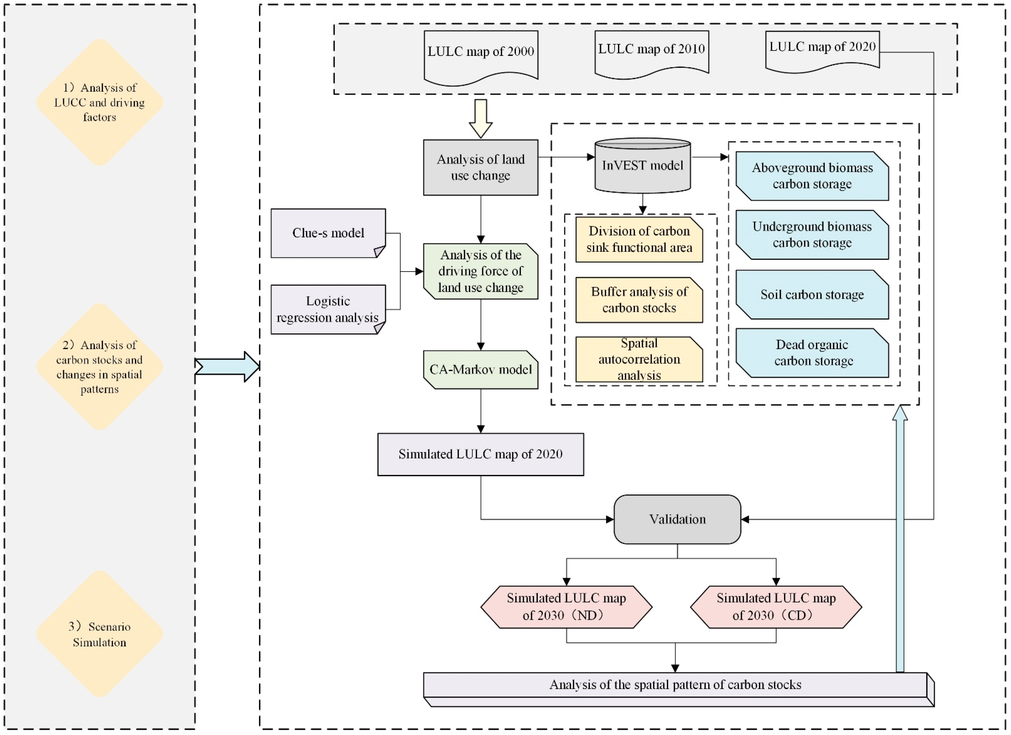
2.1. Study Framework

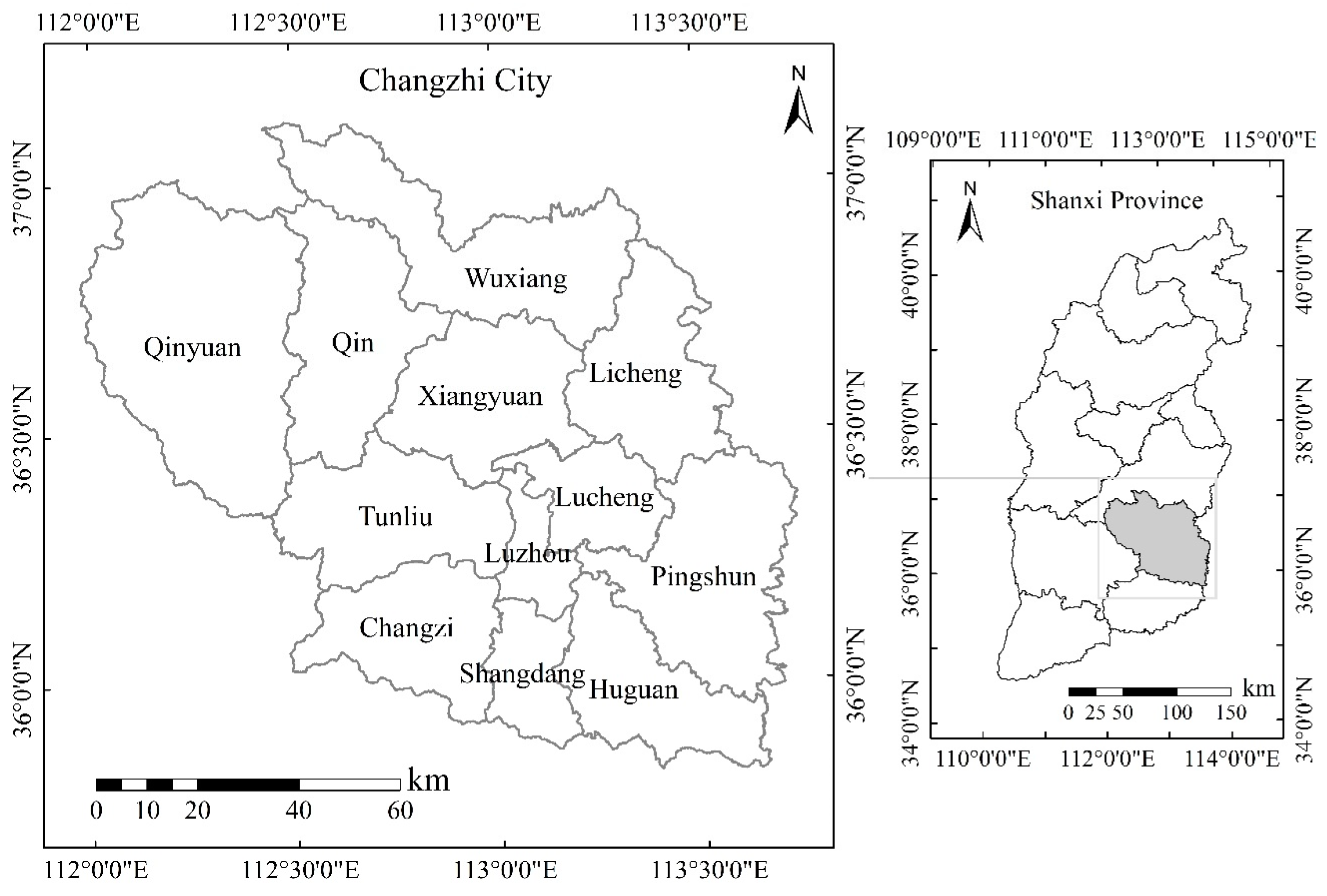
The methodological framework used for the research is shown in Figure 1. The first stage of the study is based on LUCC in Changzhi from 2000 to 2020. Firstly, the area of each land-use type was statistically analyzed through ArcGIS software, and the land-use transfer matrix was used to analyze the transfer of land types. Finally, the InVEST model was used to calculate the carbon stock changes in Changzhi City at three time points based on the carbon stocks of each land-use type and conduct the division of carbon sink functional areas using ArcGIS software. The second stage was to use ArcGIS software to conduct zoning statistics of carbon stock in Changzhi city and then import it into GeoDa software to conduct spatial correlation of carbon stock changes in regional spatial locations. Finally, based on the 2030 land-use simulation of Changzhi, LUCC and carbon stock changes were again analyzed using ArcGIS software and the InVEST model, highlighting the focus areas for future ecological management. For the simulation of the land-use pattern in Changzhi in 2030, two scenarios were defined to describe the LULC for 2030: Natural Development (ND) and Conservation Development (CD) scenario. The ND scenario was based on the supposition of maintenance of LULC conversion rates over the last 10 years (2010–2020) in the studied area. The CD scenario was based on setting up basic farmland areas, nature reserve areas, and ecological protection red line areas as restricted development areas.

2.2. Study Area

Changzhi city (35°49′–37°07′ N, 111°59′–113°44′ E) is southeast of Shanxi Province, China, at the junction of Shanxi, Hebei, and Henan (Figure 2). The warm temperate semi-humid continental monsoon climate is remarkable; the average altitude is 1000 m, and the average annual rainfall is 537.4–656.7 mm, mainly concentrated in June–August. The annual evaporation is 877.1–1124.8 mm, and the annual mean temperature is 4.9 and 10.4 °C Changzhi has jurisdiction over four districts and eight counties, with 13,955 km². The terrain of the territory is higher in altitude in the southeast and northwest, and lower in the middle, showing a basin shape in general. The whole territory is densely covered by a river network, with the Zhuozhang River and Fen River running through it. The vegetation resources are rich, mainly coniferous and broad-leaved mixed forest. Changzhi is “prosperous because of coal” as a typical coal resource-based city. The coal exploration area exceeds 3000 km², and the coal-bearing area reaches 8500 km², accounting for 61% of the city’s area, and has identified reserves of 29.3 billion tons. The output of raw coal frequently ranks among the top five in the country, reaching 139.21 million tons in 2020, with a gross domestic product of RMB 171.16 billion, ranking second in Shanxi Province, with permanent residents of about 3.18 million. Currently, the LULC is dominated by cultivated land and forest land, and the overall distribution is in the pattern of forest land—cultivated land—forest land. However, the artificial surface area has expanded dramatically in the past two decades, and the area of cultivated land has a significant downward trend.

2.3. Source of Data

The surface cover data of the study area in 2000, 2010, and 2020 are from GLOBALAND30 (resolution 30 m) (www.globallandcover.com (accessed on 24 April 2022)). Land-use type codes are cultivated land (1), forest land (2), grassland (3), shrubland (4), wetland (5), water body (6), and artificial surface (7). The images for land-cover classification of development and update of GlobeLand30 are mainly 30-m multispectral images, including TM5 ETM+, and OLI multispectral images of Landsat (USA) and HJ-1 (China Environment and Disaster Reduction Satellite), the 16-m resolution GF-1 (China High-Resolution Satellite) multispectral image are also used for GlobeLand30 2020. The total accuracy of GlobeLand30 2020 is 85.72% and the Kappa coefficient is 0.82. The socio-economic statistical data, annual rainfall data, and annual average temperature of the study area are all derived from the “Changzhi City Statistical Yearbook” and obtained through ArcGIS software interpolation; Digital elevation model (resolution 30 m), published by the Geospatial Data Cloud platform (http://www.gscloud.cn/ (accessed on 1 April 2022)), the slope data are extracted from the DEM data. The data on river systems, roads, and settlements come from the Resource Environmental Science and Data Center (http://www.resdc.cn/ (accessed on 29 April 2022)). The overall urban planning of Changzhi City comes from the Changzhi Municipal Government, and the vector data of the boundaries of administrative districts at all levels come from the third national land survey database of Changzhi City. The data on the boundaries of mining areas, basic farmland protection red lines, ecological protection red lines, nature reserves, geological disaster sites, and coal mining subsidence areas come from the Shanxi Provincial Department of Natural Resources.

2.4. Analysis of Land Use and Land Cover (LULC) Change

Based on three land-use status maps of Changzhi City in 2000, 2010, and 2020 (Figure 3), this paper uses ArcGIS software to count the area of each land-use type in the last 20 years and analyzes the land-use transfer matrix with the help of chord diagrams to reflect the land-use transfer in the study area.

2.5. Analysis of the Driving Force of LUCC

The term “binary” in binary logistic refers to the fact that the dependent variable is a dichotomous variable and logistic refers to the logit transformation of the target probability. This avoids the structural shortcomings of linear probability models. Logistic models are therefore often used to analyze land-use change, where the outcome of land-use change is either a change or no change, that is, a dichotomous variable Y, with “1” indicating a change and “0” indicating no change, and a series of independent variables Xi can be used to explain the causal relationship between them. The land-use change drivers were examined in three steps in this study: first, the raster data of each land type are binarized using ArcGIS software and then converted into ASCII codes and imported into the Clue-S model; second, the converting module in Clue-S was used to generate data on each class and its drivers; and finally, the data were imported into SPSS software for logistic regression analysis. The binary logistic regression model enables regression modeling of binary dependent and independent variables, creating corresponding regression models.

$$\log it\left(P_i\right)=In\left(\frac{P_i}{1-P_i}\right)=\alpha +{\beta }_1{x}_{1i}+{\beta }_2{x}_{2i}+···+{\beta }_z{x}_{zi}$$

(1)

where P is the probability of the change of the ith land type, α is a constant term, and β is a regression coefficient.

The ratio of the probability of conversion to non-conversion of a land class in this study is called the event occurrence ratio (odds).

$$\frac{P_i}{1-P_i}=exp(\alpha +{\beta }_1{x}_{1i}+{\beta }_2{x}_{2i}+···+{\beta }_z{x}_{zi})$$

(2)

The incidence ratio is exp (β), which represents the multiple changes in the incidence ratio of the event for each unit increase in the explanatory variable (exp (β) = 1, the incidence ratio is constant, exp (β) > 1, the incidence ratio increases, and vice versa). Pontius et al. used the ROCs (relative operating characteristics) method to test the goodness of fit of the regression model, which is generally considered good when the ROC is ≥0.7 [31].

2.6. CA-Markov Model

The Markov model is based on probabilistic knowledge and is used to investigate the possibility of things transitioning from state A to state B. Based on existing laws, it then makes predictions state of things, particularly quantitative predictions. In this study, the driving factors of LUCC are incorporated into the model, and the AHP (Analytic Hierarchy Process) method is combined to improve the performance of the model in terms of simulation and prediction. The Markov model equation is as follows:

$$S_{t+1}=S_t\times P_{ij}$$

(3)

where $S_t$ and $S_{t+1}$ are the LUCC status at the time t and t + 1, respectively; $P_{ij}$ is the transfer probability matrix.

The cellular automaton (CA) model is a dynamical model that simulates the spatiotemporal evolution of complex systems by interacting between cells with different spatiotemporal characteristics. It consists of cell space and cell dimensions, state sets, transfer rules, and domain scope [32]. The most crucial of these is determining the cell transfer rules:

$$W_{ \left(t,t+1\right)}=f \left(W_t, N\right)$$

(4)

where W is the cell’s finite and discrete state set; N is the cellular field; t and t + 1 represent different moments; f is the local space cell transformation rule.

The Markov model is focused on quantitative changes in land-use prediction and cannot guarantee spatial pattern prediction accuracy. On the other hand, the CA model is focused on meta-cell local interactions but cannot accurately predict quantitative changes. As a result, the CA model can be effectively combined with the Markov model to compensate for each model’s shortcomings and achieve dual prediction of spatial location and quantitative changes in land-use types. In this paper, we used the CA-Markov model in IDRISI32 software to predict the spatial pattern of land use in Changzhi City in 2020 with 2010 as the starting year, and compared it with the actual land-use data in 2020 to verify the reliability of the CA Markov model simulation. We further predicted the land-use spatial pattern in 2030 with 2020 as the starting year. According to the functional requirements of the CA Markov model, the simulation and prediction process has the following key steps. (1) Conversion rules: We used the spatial land-use data of 2000, 2010, and 2020 to obtain the land-use transfer area matrix and transfer probability matrix for 2000–2010 and 2010–2020, which were used as the conversion rules for predicting the spatial pattern of land use in 2020 and 2030. (2) Production of a land-use suitability atlas for Changzhi: The probability map of the spatial distribution of each land-use type was calculated by binary logistic regression analysis, and then the set editor module in IDRISI32 software was used to generate the suitability atlas. (3) Construction of CA filters: Based on related studies, we used a 5 × 5 filter. (4) Determination of starting nodes and CA cycle number: We set the CA cycle number to 10 based on the land-use pattern in 2010, and combined the land-use suitability atlas from 2000 to 2010 and the land-use transfer probability matrix to simulate the land-use pattern in 2020. Based on this, we set the CA cycle number to 10 based on the land-use pattern in 2020 as the starting year, and combine the land-use suitability atlas and land-use transfer probability matrix for 2010–2020 to simulate the land-use pattern in 2030.

2.7. Regional Carbon Storage Assessment Based on InVEST Model

2.7.1. Estimation of Carbon Storage

The InVEST model is widely used to quantify changes in ecosystem value at the time of different land-use scenarios. This study uses the carbon storage module of the InVEST model to assess changes in carbon stocks in Changzhi. This module generates ecosystem carbon stock data based on land-use data and carbon density data in the study area. It divides the ecosystem carbon stocks into four basic carbon pools: aboveground biomass carbon ($C_{v\_above}$), underground biomass carbon ($C_{v\_below}$), and soil organic carbon ($C_{v\_soil}$), and litter carbon ($C_{v\_litter}$), and assesses the regional ecosystem carbon stocks based on the spatial distribution pattern of each vegetation cover type and its corresponding carbon density, and outputs a spatial distribution map of carbon stocks. The aboveground biomass carbon pool includes the carbon stored in all living vegetation (bark, trunk, branches, leaves, etc.) above the surface; the underground biomass carbon pool refers to the carbon stored in the living root systems of plants; the soil organic carbon pool generally refers to the organic carbon stored in mineral and organic soils; and the litter carbon pool represents the carbon stored in apoplastic matter and dead plants [33].

$$C_v=C_{v\_above}+C_{v\_below}+C_{v\_soil}+C_{v\_litter}(v=1,2,3\cdots , \mathrm{n})$$

(5)

$$C_0={{\displaystyle \sum }}_{v=1}^n \left(S_v\times C_v\right)$$

(6)

where $C_v$ is the carbon density of LUCC type v (t/ha), $C_0$ is the total carbon storage in the study area (t); $S_v$ is the area of LUCC type v (ha).

2.7.2. Carbon Density Correction

Numerous studies have shown a significant linear relationship between carbon density and climatic factors since vegetation cover, stand species, stand density, and hydrology influence above and below-ground biomass density, while temperature and precipitation influence vegetation cover, stand species, and stand density, and water content. Tang et al. developed a regression model for the relationship between biological and soil carbon density and mean annual precipitation and mean annual temperature under different climatic conditions based on data from 14,371 measured sample sites in China, verifying that biological and soil carbon density was highly correlated with climatic factors, with carbon density being inversely proportional to temperature and positively proportional to rain [34]. Based on the study of carbon storage density of six major land types in China by Kerang Li, Xianli Xie, Xuli Tang, et al. [34,35,36], the carbon density was corrected by the average annual precipitation and average annual temperature in Changzhi City to obtain the biological carbon density and soil carbon density of six major land-use types in Changzhi City using the following correction formula [37,38].

Regression model considers temperature (MAP ≥ 400 mm)

$$C_{BP}=-0.4MAT+43.0$$

(7)

$$C_{SP}=-0.03MAT+2.03$$

(8)

$$C_{LP}=-3.4MAT+15.7$$

(9)

Regression model considers precipitation (MAT ≤ 10 °C)

$$C_{BT}=0.03MAP+14.4$$

(10)

$$C_{SP}=0.07MAP+79.1$$

(11)

$$C_{LP}=0.001MAP+0.58$$

(12)

Regression model considers precipitation (MAT ≥ 10 °C)

$$C_{BT}=0.02MAP+5.87$$

(13)

$$C_{SP}=0.03MAP+45.3$$

(14)

$$C_{LP}=0.004MAP+0.85$$

(15)

where MAP and MAT signify average annual rainfall (mm) and the average annual temperature (°C) in Changzhi, respectively; $C_{BP}$ and $C_{BT}$ signify carbon density (t/ha) corrected for MAP and MAT, respectively; $C_{SP}$ and $C_{ST}$ signify soil carbon density (t/ha) corrected for MAP and MAT, respectively; and $C_{LP}$ and $C_{LT}$ signify deadfall carbon density corrected for MAP and MAT, respectively. Changzhi’s MAP and MAT were assigned to the corresponding relationships as ${C^{\prime }}_{BP}$, ${C^{\prime }}_{BT}$, ${C^{\prime }}_{SP}$, ${C^{\prime }}_{ST}$, ${C^{\prime }}_{LP}$, ${C^{\prime }}_{LT}$, while the national MAP and MAT were assigned as ${C^{″}}_{BP}$, ${C^{″}}_{BT}$, ${C^{″}}_{SP}$, ${C^{″}}_{ST}$, ${C^{″}}_{LP}$, ${C^{″}}_{LT}$.

Correction model:

$$K_{BP}=\raisebox{1ex}{${C^{\prime }}_{BP}$}\!\left/ \!\raisebox{-1ex}{${C^{″}}_{BP}$}\right.;K_{BT}=\raisebox{1ex}{${C^{\prime }}_{BT}$}\!\left/ \!\raisebox{-1ex}{${C^{″}}_{BT}$}\right.;$$

(16)

$$K_{SP}=\raisebox{1ex}{${C^{\prime }}_{SP}$}\!\left/ \!\raisebox{-1ex}{${C^{″}}_{SP}$}\right.;K_{ST}=\raisebox{1ex}{${C^{\prime }}_{ST}$}\!\left/ \!\raisebox{-1ex}{${C^{″}}_{ST}$}\right.;$$

(17)

$$K_{LP}=\raisebox{1ex}{${C^{\prime }}_{LP}$}\!\left/ \!\raisebox{-1ex}{${C^{″}}_{LP}$}\right.;K_{LT}=\raisebox{1ex}{${C^{\prime }}_{LT}$}\!\left/ \!\raisebox{-1ex}{${C^{″}}_{LT}$}\right.;$$

(18)

$$K_B=Average(K_{BP}+K_{BT})$$

(19)

$$K_S=Average(K_{SP}+K_{ST})$$

(20)

$$K_L=Average (K_{LP}+K_{LT})$$

(21)

where $K_{BP}$, $K_{BT}$, $K_{SP}$, $K_{ST}$, $K_{LP}$, $K_{LT}$ are correction factors for biomass carbon density considering precipitation, biomass carbon density considering temperature, soil carbon density considering precipitation, soil carbon density considering temperature, deadfall carbon density considering precipitation, and deadfall carbon density considering temperature, respectively.

2.8. Spatial Analysis

The regional spatial features of carbon storage in Changzhi were mined using grid analysis. Grid analysis usually uses a triangle grid, quadrilateral grid, hexagon grid, etc. The hexagonal grid is a superior choice when considering the boundary impact of grid shapes, the same distance from the center of mass in all six directions, and the minor sample error [39,40]. According to the actual situation of Changzhi City, a positive hexagon with side length of 1 km was selected in ArcGIS software for carbon stock zoning statistics and then imported into Geoda software for spatial autocorrelation analysis. Spatial autocorrelation is used to describe the spatial aggregation of geographic phenomena, and is a basis for determining whether there is potential interdependence between variables within the same distribution area, and can be divided into global and local spatial autocorrelation. Global spatial autocorrelation is a description of the overall distribution of a phenomenon, and can determine the existence of spatial agglomeration of the phenomenon within a region, but cannot specify the location of the agglomeration exactly; local spatial autocorrelation can further explore the analysis of the existence of spatial heterogeneity and find the spatial location of the agglomeration center. The global spatial autocorrelation in this paper refers to testing the spatial correlation between carbon stocks and neighboring grid attribute values in the global perspective of the study area. The results are reflected by the global Moran’s I, which takes values from −1 to 1. I > 0 means that the variables are positively correlated in space, showing spatial agglomeration characteristics, while the opposite is a negative correlation, showing spatial isolation characteristics. The spatial autocorrelation of the variables is usually tested by the Z value. Finally, the results of Moran’s I analysis in GeoDa software were imported into ArcGIS software and combined with the results of Moran’s I analysis to create LISA clustering maps [41].

$$I=\frac{{{\displaystyle \sum }}_{i=1}^n{{\displaystyle \sum }}_{j=1}^n{w}_{ij} \left(x_i-\overline{x}\right) \left(x_j-\overline{x}\right)}{{\sigma }^2{{\displaystyle \sum }}_{i=1}^n{{\displaystyle \sum }}_{j=1}^n{w}_{ij}}$$

(22)

where $x_i$, $x_j$ is the attribute value of the grid units; n is the total number of units; $\overline{x}$ is the average carbon storage of the grid unit; ${\sigma }^2=\frac{1}{n}{\displaystyle \sum }_1^n(x_i-\overline{x}{)}^2$ is the sample variance; $w_{ij}$ is the spatial weight matrix.

The value range of Global Moran’s I is [−1, 1]. The value is positive, indicating that the spatial correlation is positive, and the higher absolute values suggest a more robust correlation and vice versa.

For studying carbon density agglomeration characteristics at a location, a local autocorrelation analysis can be used, with the formula:

$$I_i=\frac{ \left(x_i-\overline{x}\right)}{{\sigma }^2}{{\displaystyle \sum }}_{j=1}^n{w}_{ij} \left(x_j-\overline{x}\right)$$

(23)

where $I_i$ is the local Moran’s I of the evaluation unit i, a positive (negative) value of $I_i$ indicating that similar (dissimilar) carbon storage areas are adjacent, the absolute value reflects the degree of proximity, and the smaller the p-value indicates a higher confidence level.

3. Result

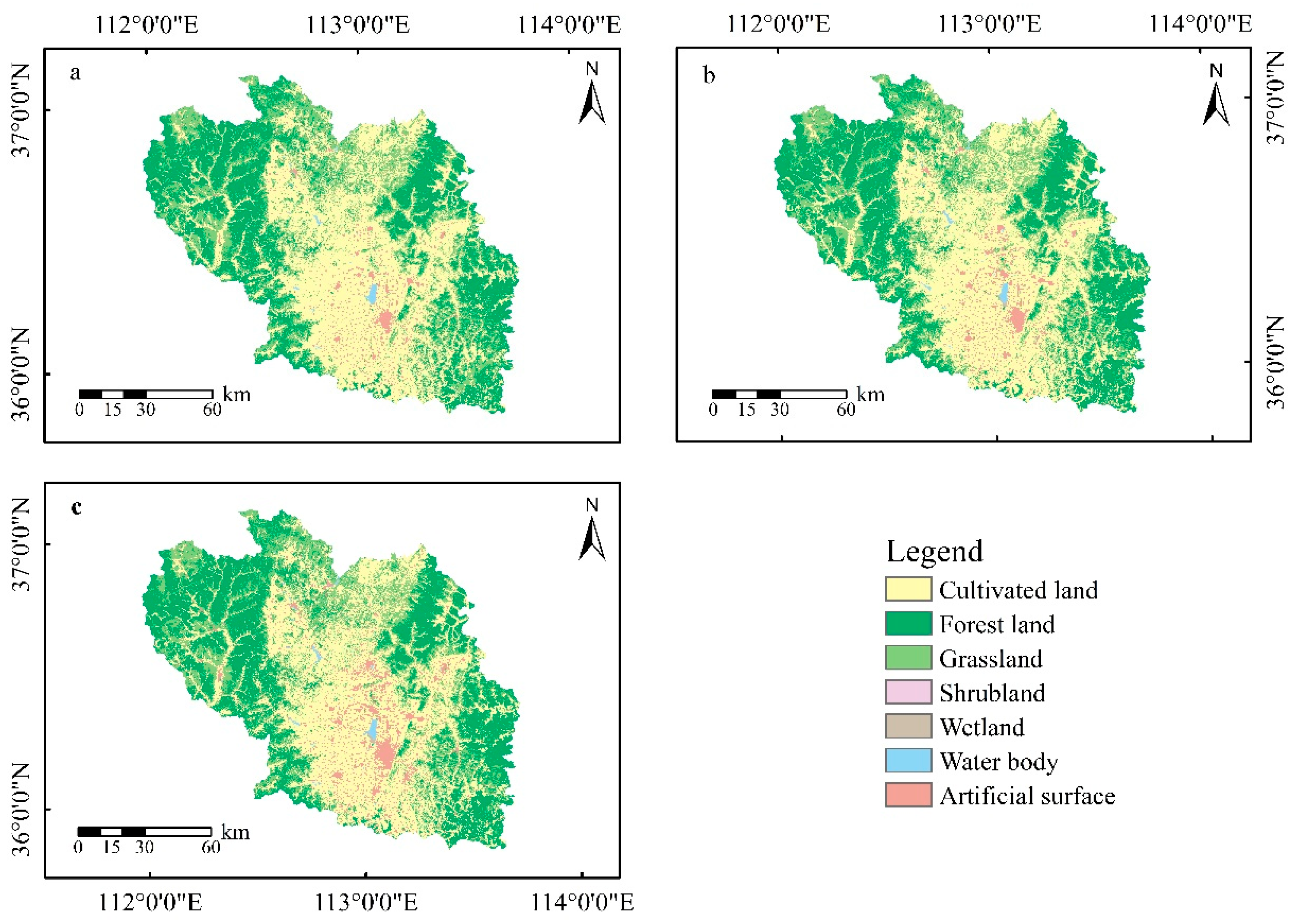
3.1. Spatio-Temporal Patterns of LUCC in Changzhi City during 2000–2020

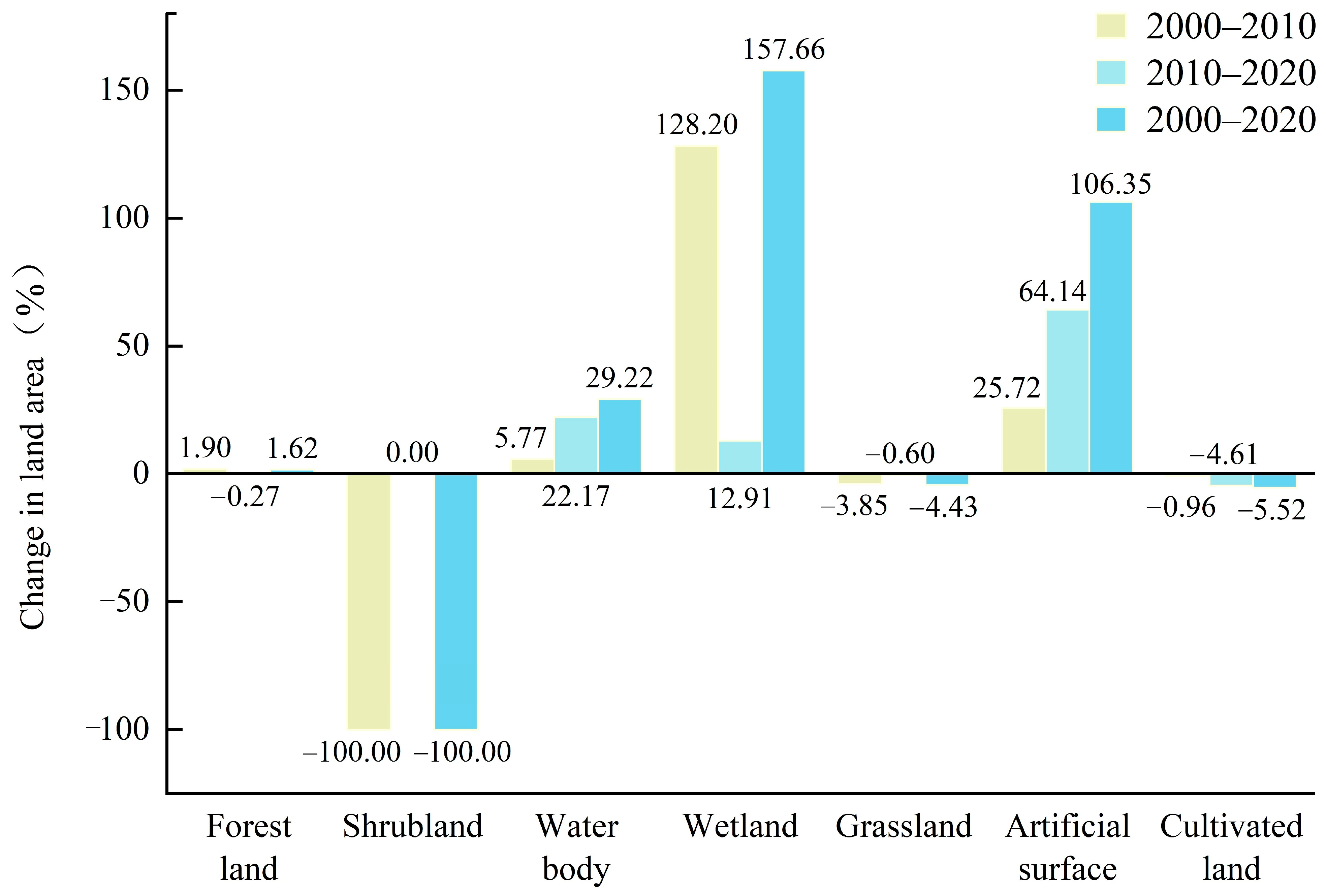
3.1.1. LUCC

The LUCC of the study area at three time points is shown in Figure 3 (2000, 2010, and 2020), with cultivated land consistently accounting for the largest area, with the proportion remaining at 40–43%, followed by forest land, grassland, and artificial surface, accounting at 30–31%, 22–24%, and 2–6%, respectively. The other three LUCC types, shrubland, wetland, and water body, accounted for about 0.5% of the total area. The changes in each land-use type are shown in Figure 4 Cultivated land and grassland area in Changzhi City have decreased in the past two decades. In the first decade (2000–2010), they decreased by 57.04 km² (0.96%) and 125.42 km² (3.85%), respectively, and in the second decade (2010–2020), they decreased by 270.14 km² (4.61%), 18.73 km² (0.60%), respectively; the forest land area increased first and then decreased, increased by 82.82 km² (1.90%) in the first decade, and decreased by 11.89 km² (0.27%) in the second decade. Since the area of shrubland, wetland, and water body areas accounts for a small proportion, the change is not noticeable compared with the total area of Changzhi City. However, the change is quite drastic compared to its area. From 2000 to 2010, the shrubland area decreased by 100% (0.10 km²), the wetland area increased by 128.2% (4.91 km²), and the water area increased by 5.72% (2.46 km²). From 2010 to 2020, the wetland area increased by 12.91% (1.13 km²), and the water body area increased by 22.00% (10.00 km²). The artificial surface area increased by 382.02 km² (106.34%) in the past two decades, and the expansion rate in the last decade was significantly faster than that in the first decade. From 2000 to 2010 and 2010 to 2020, the artificial surface increased by 92.38 km² (25.72%) and 289.64 km² (64.14%). To sum up, during the period from 2000 to 2020, the area of cultivated land and grassland in Changzhi City continued to decrease; while the development of forest land and water body area was relatively stable, the growth of wetland area mainly occurred in the first decade, and the area of the artificial surface has been growing at speed during the 20 years.

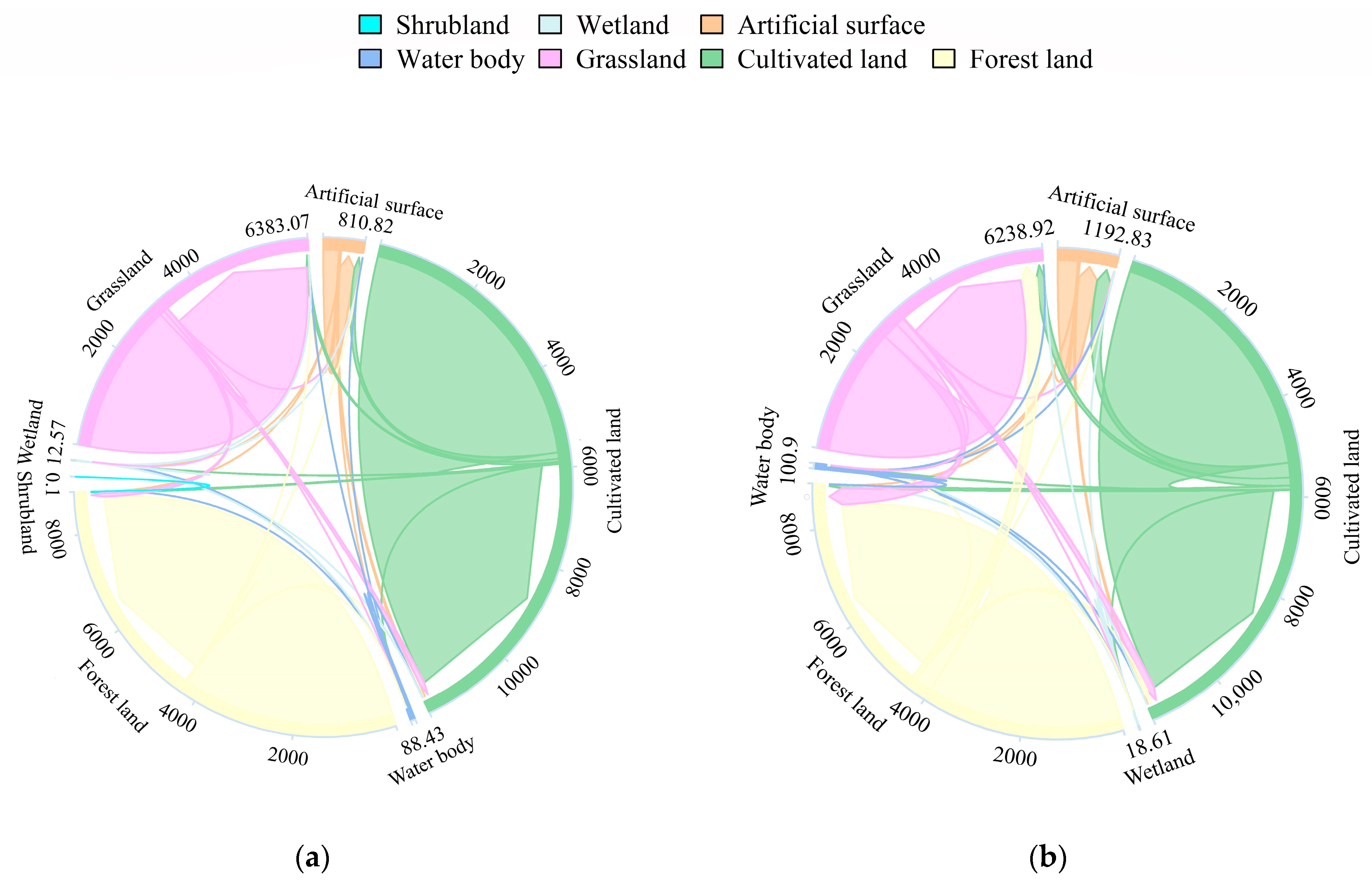
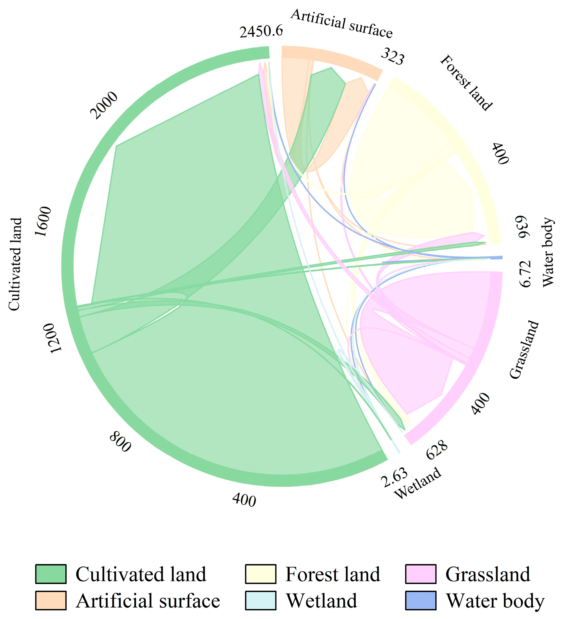
3.1.2. LULC Types Conversion

Figure 5 shows the transfer of land-use types in Changzhi City over the past two decades. The main land-use type transfers occurred between cultivated land to the artificial surface, grassland to cultivated land, and grassland to forest land. Among the conversion of non-artificial surfaces to artificial surfaces, cultivated land accounts for 94.94% because rapid urbanization has taken up large areas of cultivated land. Despite China implementing a strict cultivated land protection system since 2005, it has not successfully limited the rapid urbanization process. Artificial surface, forest land, and grassland are the primary sources of conversion of non-cultivated land to cultivated land, accounting for 22.44%, 16.83%, and 57.23%; in the conversion of non-forest land to forest land, the primary sources are cultivated land and grassland, accounting for 28.55% and 70.83%, which may be associated to the State’s forest land protection policies implemented since 2005, such as the ban on deforestation, afforestation, and returning farmland to forest, etc. Implementing these protection policies has guaranteed the stable growth of forest land area. The conversion to grassland, wetland, and water body areas, with cultivated land being the main contributor, accounted for 92.79%, 81.14%, and 75.01%. The conversion of cultivated land to forest land and grassland accounted for 40% of the total, which is attributed to China’s farmland return to forest program implemented in 1999, which promoted the conversion of cultivated land with slopes greater than 25° to forest land and grassland. During the period 2010–2020, the area of the artificial surface increased by 64.14%, with cultivated land contributing the most at 93.11%, indicating that the cultivated land protection system is finding it difficult to limit the expansion of artificial surface areas and conversion of cultivated land as a result of urbanization. The more conversions to cultivated land were to grassland, forest land, and artificial surfaces, accounting for 57.46%, 30.38%, and 11.17%, respectively, with a 70.8% increase in total conversions compared to the previous decade; this is due to the issuance of The Ministry of Land and Resources’ Circular on Issues Relating to the Full Implementation of Arable Land Replenishment before Occupation. The largest contributor to the conversion to forest land was grassland, accounting for 81.42%; the most conversion of grassland was to forest land and cultivated land, accounting for 67.04% and 32.76%, respectively; and the main contributors to the transfer to the water body and wetland remained cultivated land, accounting for 77.32% and 52.78%, respectively.

The above shows that in Changzhi, development and construction and forest land expansion have primarily occurred through the occupation of cultivated land and grassland over the last 20 years, with relatively stable wetland and water body growth.

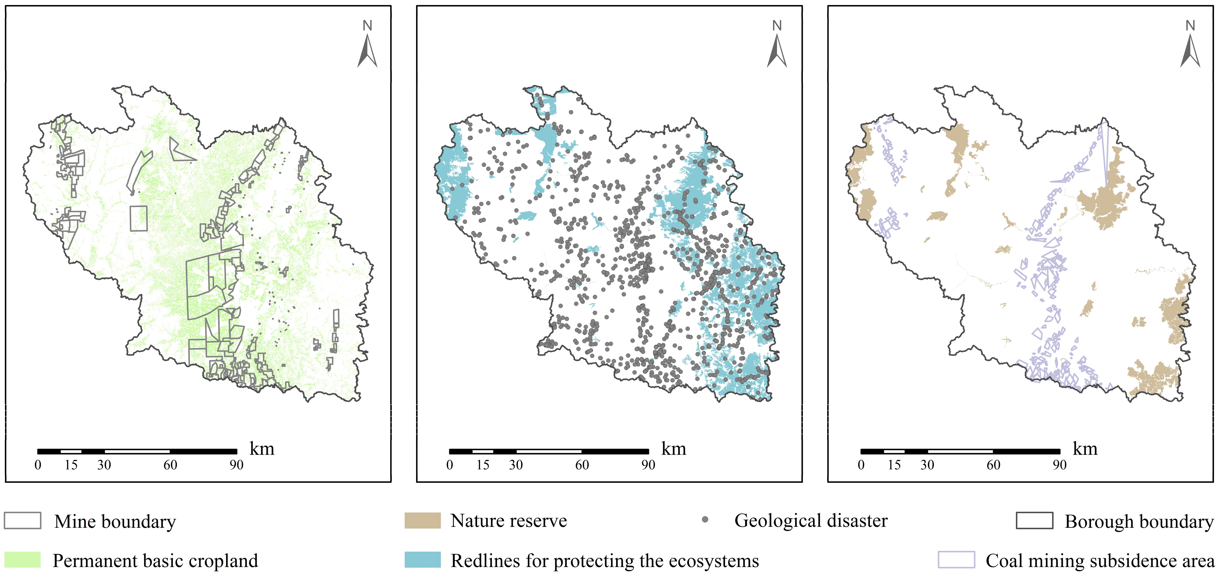
3.1.3. LULC Types Conversion in Mining Areas

Changzhi is a typical coal resource city, with a well-developed coal industry and opencast mining as the primary mining method. Large-scale mining will inevitably harm the already fragile ecosystem and change the rate and direction of land-use succession in the region. Opencast mining in Changzhi directly changes the land-use types and surface landscape in the short term, leading to frequent geological disasters (ground cracks, ground subsidence, landslides, debris flows, and landslides) (Figure 6). The subsidence map illustrates that in Changzhi, most geological hazard locations and subsidence zones are centered within mining areas. According to Changzhi City’s Bureau of Natural Resources statistics, as of 2019, the total area of land occupied and damaged by mining in Changzhi City was 160.49 km², and the damage factor of coal mines was 16.87 km²/billion tons. Geological disaster sites and coal mining sinkholes are the results of ecological damage. Both can cause loss of carbon sequestration capacity of ecosystems and, in severe cases, change the land-use type, resulting in a complete loss of carbon sequestration capacity. Statistics on changes in land types within Changzhi’s mine boundary from 2000 to 2020 show that the area of cultivated land lost within the mine boundary over the 20 years was nearly 10%, nearly twice the proportion of cultivated land lost in the city over the same period (5%) (

Table 1. Transfer matrix of land use in mining areas of Changzhi City between 1995 and 2015 (km²).

2020	2000
	Cultivated Land	Forest Land	Grassland	Wetland	Water Body	Artificial Surface	Total
Cultivated land	1123.947	7.143	18.256	0.185	1.118	14.099	1164.748
Forest land	11.296	275.726	35.867	0.000	0.000	0.097	322.985
Grassland	22.011	29.261	257.668	0.004	0.004	0.380	309.327
Wetland	1.234	0.103	0.070	0.472	0.019	0.000	1.898
Water body	2.491	0.042	0.735	0.068	1.107	0.004	4.447
Artificial surface	124.923	0.819	5.739	0.000	0.024	88.691	220.197
Total	1285.901	313.094	318.334	0.728	2.273	103.271	2023.602

). The artificial surface has increased by almost 113%, of which 95% is from cultivated land (Figure 7). Wetland areas have increased by more than 160%, and water body areas have increased by more than 95%, likely due to regional land-use changes caused by coal mining subsidence. The 5% increase in the forest within the mine boundary could be attributed to ecological restoration projects following the mining operation. Even though the mine’s forest land and wetland areas have grown, they have not been able to compensate for the carbon loss caused by the loss of large areas of cultivated land, with a total carbon loss of 77,497 t within the mine boundary over 20 years.

3.2. Driving Factors of LUCC

Concerning existing studies and the actual situation in Changzhi, 19 potential drivers were chosen for analysis, including natural factors such as elevation (x1), slope (x2), slope aspect (x3), average annual temperature (x4), average annual precipitation (x5), soil type (x6), and landform type (x7); socioeconomic factors such as population density (x8) and GDP data (x9); and transport location accessibility factors such as distance to railways (x10), distance to residential area (x11), distance to national highway (x12), distance to expressway (x13), distance to provincial highway (x14), Distance to county road (x15), distance to township road (x16), distance to river (x17), distance to reservoir (x18), distance to county center (x19). The x1, x2, x3, x4, x5, x8, and x9 factors are grouped in ascending order into five categories I to V. x6 is divided into 10 categories I to X. Category I is water; category II to X is fluvo-aquic soil, skeletal soils, cinnamon soils, red clay soils, cultivated loessial soil, mountain meadow soils, litho soils, alluvial soils, and brown earth, x7 is divided into five categories I~V, followed by large undulating mountains, loess hills, plains, hills, and medium rolling hills.

Clue-S model and binary logistic regression were used to analyze the drivers of LUCC for each of the six land types: cultivated land, forest, grassland, wetland, water body, and artificial surface, and the B-value, Exp-value, and p-value of the drivers are shown in

Table 2. Analysis of the drivers of different land-use types.

	Cultivated Land			Forest Land			Grassland			Wetland			Water Body			Artificial Surface
	B	Exp	p	B	Exp	p	B	Exp	p	B	Exp	p	B	Exp	p	B	Exp	p
x1	−0.0043	0.996	0.000	0.0033	1.003	0.000	−0.0005	1.000	0.001	-	-	0.373	-	-	0.686	−0.0031	0.997	0.000
x2	−0.1032	0.902	0.000	0.7130	1.074	0.000	0.0324	1.033	0.000	-	-	0.676	−0.4137	0.661	0.000	−0.1125	0.894	0.000
x3	-	-	0.615	0.0009	1.001	0.000	-	-	0.085	-	-	0.688	−0.0239	0.976	0.000	-	-	0.827
x4	-	-	0.159	0.1470	1.158	0.002	−0.4165	0.659	0.000	-	-	0.239	0.4457	1.562	0.080	0.2738	1.315	0.000
x5	0.0196	1.020	0.000	-	-	0.707	-	-	0.267	-	-	0.270	-	-	0.766	-	-	0.173
x6	0.1284	1.137	0.000	−0.1223	0.885	0.000	0.0412	1.042	0.001	-	-	0.398	−0.0676	0.846	0.052	-	-	0.691
x7	−0.0582	0.943	0.001	0.0664	1.069	0.000	0.1552	1.068	0.000	-	-	0.380	-	-	0.456	-	-	0.282
x8	−0.0005	0.999	0.000	−0.0015	0.999	0.000	−0.0010	0.999	0.000	-	-	0.553	-	-	0.291	0.0006	1.001	0.000
x9	0.0000	1.000	0.000	0.0000	1.000	0.000	0.0000	1.000	0.000	-	-	0.615	-	-	0.759	0.0000	1.000	0.000
x10	0.0000	1.000	0.033	0.0000	1.000	0.000	-	-	0.466	-	-	0.241	-	-	0.403	-	-	0.332
x11	0.0000	1.000	0.008	0.0000	1.000	0.004	-	-	0.732	-	-	0.458	-	-	0.929	−0.0002	1.000	0.000
x12	-	-	0.339	0.0000	1.000	0.000	0.0000	1.000	0.000	−0.0002	1.000	0.098	-	-	0.340	0.0000	1.000	0.038
x13	0.0001	1.000	0.014	0.0000	1.000	0.000	0.0000	1.000	0.000	-	-	0.796	-	-	0.573	-	-	0.126
x14	0.0000	1.000	0.000	0.0000	1.000	0.000	0.0000	1.000	0.000	-	-	0.379	-	-	0.068	−0.0001	1.000	0.000
x15	−0.0001	1.000	0.000	0.0001	1.000	0.000	0.0000	1.000	0.005	-	-	0.983	-	-	0.705	−0.0001	1.000	0.000
x16	−0.0001	1.000	0.000	0.0001	1.000	0.000	0.0000	1.000	0.000	-	-	0.098	-	-	0.394	−0.0001	1.000	0.003
x17	-	-	0.172	0.0000	1.000	0.012	0.0000	1.000	0.015	-	-	0.689	−0.0015	0.999	0.000	-	-	0.505
x18	0.0001	1.000	0.000	−0.0001	1.000	0.000	0.0000	1.000	0.000	−0.0047	0.995	0.007	−0.0003	1.000	0.005	-	-	0.573
x19	0.0000	1.000	0.000	0.0001	1.000	0.001	0.0000	1.000	0.000	−0.0002	1.000	0.036	-	-	0.943	-	-	0.502
ROC	0.837			0.858			0.683			0.994			0.973			0.900

p value indicates the significance detection range, if the value is less than 0.05, it will pass, otherwise, it will not pass the significance test.

. The regression coefficients of the drivers are B values, where Exp (B) represents the incidence ratio and probability of change for each land-use type for each unit change in the driver. The logistic model’s goodness of fit is generally validated using the ROC curve, with the ROC taking a value range of 0.5 ~ 1. It is generally assumed that the regression model fits better when the ROC is 0.7.

The results show that the study area’s cultivated land distribution is positively correlated with x5, x6, x9, x10, x11, x13, x14, x18, and x19; negatively correlated with x1, x2, x7, x8, x15, and x16; and not correlated with x3, x4, x12, and x17. Of these, x6 has the most significant impact on cultivated land distribution, with the probability of cultivated land distribution increasing by 13.7% for each unit increase in the code corresponding to x6. x1, x2, x3, x4, x7, x9, x10, x11, x12, x13, x14, x15, x16, x17, and x19 positively correlated with forest land distribution, while x6, x8, and x18 had a negative correlation. Of these, x4 had the most significant impact on forest land distribution, with the probability of forest land distribution increasing by 15.8% for each unit increase in the code corresponding to x4. x2, x6, x7, x9, x12, x13, x14, x15, x16, x17, x18, and x19 positively correlated with grassland distribution, while x1, x4, and x8 had a negative correlation. Of these, x4 had the most significant impact on grassland distribution, with the probability of grassland distribution decreasing by 34.1% for each unit increase in the code corresponding to x7. Wetland distribution correlated negatively with x12, x18, and x19. For each unit increase in the code corresponding to x4, the probability of wetland distribution increased by 0.5%. Water body distribution correlated positively with x4, with a negative correlation with x2, x3, x6, x17, and x18. Of these, x4 had the most significant impact on water body distribution, with the probability of water body distribution increasing by 56.2% for each unit increase in the code corresponding to x4. Artificial surface distribution negatively correlated with x1, x2, x11, x14, x15, and x16 and had a positive correlation with x4, x8, x9, and x12. Of these, x4 had the most significant impact on artificial surface distribution, with the probability of artificial surface distribution increasing by 31.5% for each unit increase in the code corresponding to x4.

Further analysis of the transfer of the eight major land-use types in the study area was conducted (

Table 3. Analysis of the drivers of land class conversion.

Variables	B	Exp	p	Variables	B	Exp	p
T12 (ROC = 0.722)				T23 (ROC = 0.669)
x2	0.0576	1.059	0.000	x1	−0.0013	0.999	0.000
x9	−0.0000	0.999	0.025	x2	−0.0210	0.979	0.002
x11	0.0001	1.000	0.004	x4	−0.4142	0.661	0.000
x16	0.0001	1.000	0.000	x12	0.0000	1.000	0.017
T13 (ROC = 0.750)				x13	0.0000	0.999	0.001
x2	0.0946	1.099	0.000	x16	−0.0001	0.999	0.000
x6	0.1084	1.115	0.038	x18	0.0000	1.000	0.007
x11	0.0001	1.000	0.012	x19	0.0000	1.000	0.009
T17 (ROC = 0.779)				T31 (ROC = 0.724)
x1	−0.0025	0.998	0.000	x1	−0.0031	0.997	0.000
x2	−0.0675	0.935	0.000	x2	−0.0271	0.973	0.004
x8	0.0006	1.001	0.000	x6	0.1136	1.120	0.015
x9	0.0000	1.000	0.000	x7	−0.2535	0.776	0.000
x10	0.0000	0.999	0.016	x9	0.0000	1.000	0.000
x11	−0.0001	0.999	0.000	x15	−0.0001	0.999	0.029
x15	−0.0001	0.999	0.010	x18	0.0001	1.000	0.003
T21 (ROC = 0.834)				x19	−0.0001	0.999	0.000
x1	−0.0476	0.995	0.000
x2	−0.0889	0.915	0.000	T32 (ROC = 0.667)
x5	0.0169	1.017	0.016	x1	0.0008	1.001	0.002
x10	0.0001	1.000	0.007	x2	0.0117	1.012	0.045
x15	−0.0001	0.999	0.011	x5	0.0196	1.020	0.000
x19	−0.0001	0.999	0.000	x6	−0.0674	0.935	0.043
T71 (ROC = 0.763)				x8	−0.0017	0.998	0.004
x8	−0.0008	0.999	0.006	x9	0.0000	0.999	0.019
x10	−0.0001	0.999	0.013	x15	0.0000	1.000	0.013
x12	0.0001	1.000	0.008	x17	−0.0001	0.999	0.003

T12: cultivated land to forest land; T13: cultivated land to grassland; T17: cultivated land to artificial surface; T21: forest land to cultivated land; T23: forest land to grassland; T31: grassland to cultivated land; T32: grassland to forest land; T71: artificial surface to cultivated land. p value indicates the significance detection range, if the value is less than 0.05, it will pass, otherwise, it will not pass the significance test.

). In the transfer of agricultural land, T12 was mainly influenced by four factors: x2, x9, x11, and x16, with slope (x2) being the most influential. 49.2% of the T12 transfer occurred within a slope of 5–15°, 27.7% occurred within a slope of 15–25°, and 12.7% occurred within a slope of 0–5°. T13 was positively correlated with factors x2, x6, and x11, with slope (x2) and soil type (x11) being the main influence, with T13 accounting for 12.9% in the 0–5° slope range and up to 79.9% in the 5–25° range, with T13 transfer accounting for 25.5% in soil type IV and 50.6% in soil type VI. T17 correlation factors are more complex; x1, x2, x10, x11, and x15 had a negative correlation with their occurrence probability, with elevation (x1) and slope (x2) being the main negative correlation factors and population density (x8) and GDP (x9) being the main positive correlation factors. 660.77 km² of agricultural land was transferred out over 20 years, with T17 accounting for 60.5%, and 52.8% of T17 occurred in the 0–5° slope range. T17 accounted for 81.6% of the 245.70 km² of agricultural land shifted within the 0–5° slope. x1, x2, x15, and x19 are negative correlates of T21 in the forest land transfer, with elevation (x1) and slope (x2) playing a major role, with 50.5% of T21 in the slope range of 5–15° and 28.5% in the range of 15–25°; 52.4% of T21 in DEM Class III, with precipitation (x5) and distance from railway (x10) being positive correlates of T21, with 47.9% of T21 occurring in precipitation (x5) Class II and 18.0% in precipitation Class V. Class II precipitation accounted for 31.3% of total cultivated area. Class V precipitation accounted for 10.4% of the total cultivated area. T23 is the most common type of forest conversion, accounting for 79.6%, and is impacted by eight factors: x1, x2, x4, x12, x13, x16, x18, and x19, with x1, x2, x4, x13, and x16 having negative relationships. The main affecting factors are slope (x2) and temperature (x4), with 41.0% of T23 occurring within the slope range of 5–15° and 36.2% occurring within 15–25°; temperature II, III, and V accounted for 80.0%. T31 was influenced negatively by x1, x2, x7, x15, and x19 in the grassland shift, with slope (x2) and landform (x7) dominating. T31 occurred in the slope ranges 5–15° (53.9%) and 15–25° (27.1%), and 29.5% of T31 occurs in large rolling hills and 35.1% in hilly areas, x6, x9, and x18 are positive influences, with soil type (x6) playing a major role, with soil type class III accounting for 8.6%, class IV accounting for 25.5%, and grade VI accounting for 51.6%. T32 accounted for 65.9% of grassland conversion, with positive influences are x1, x2, x5, and x15, with slope (x2) and precipitation (x5) being the key influencing factors, the slope ranges of 5–15° and 15–25° accounted for 37.1% and 36.1%, respectively, and the total percentage of precipitation categories II, III, and V was 82.6%; the negative affecting factors were x6, x8, x9, and x17, with soil type (x6) being the main influence, with soil type IV accounting for 44.5% and VI accounting for 29.4%. T71 accounts for 95.1% of all artificial surface transfers. Population density (x8) has the biggest influence on T71, followed by x10 and x12. Among the six LUCC types and the eight major LUCC type transfers, all regression models had ROC values greater than 0.7, except for the regression model’s ROC values between 0.66–0.69 for grassland, grassland to forest land, and forest land to grassland, indicating that the logistic regression models associated with grassland were poorly fitted.

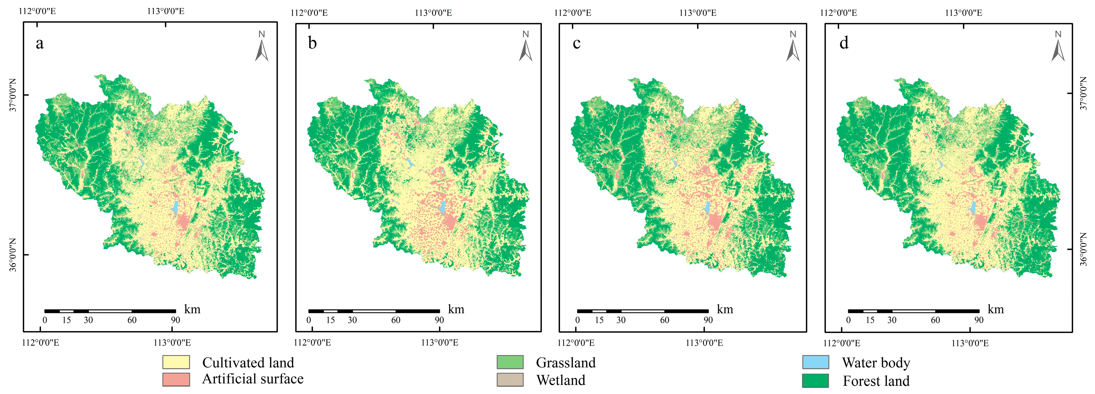
3.3. Validation of the Model and LULC Simulation for the ND and CD Scenarios

By comparing the predicted land-use status in 2020 (Figure 8a) with the actual land-use status map in 2020 (Figure 8b), the model’s prediction accuracy for land-use change in Changzhi City is verified. It is verified that the Kappa coefficient is 87%, and the overall accuracy is 89%. The calculation result of the Kappa coefficient reflects the similarity between the simulated value and the current situation, and more than 80% is considered to be a very accurate prediction tool. Therefore, it is reliable to study land-use change in Changzhi City through this model [43].

Figure 8 shows the LULC simulation results for 2030 under the nature scenario (Figure 8c) and CD scenario (Figure 8d). The ND does not set restricted areas, and the land-use pattern in 2030 is obtained by simulating the land-use transfer probability according to 2010–2020. The CD scenario is to set ecological reserves, nature reserves, and basic farmland areas as restricted areas under the coordination of economic development and environmental protection according to different policy requirements.

Compared with 2020 (

Table 4. Changes in land use and land cover (LULC) between 2020 and 2030 in Changzhi City.

LULC Types	Actual LULC 2020		Simulated LULC in 2030 under the Assumption of the ND and CD Scenarios
			ND		CD
	km2	%	km2	%	km2	%
Cultivated land	5595.15	40.11%	4976.04	35.67%	5421.72	38.86%
Forest land	4439.03	31.82%	4634.27	33.22%	4545.80	32.58%
Grassland	3110.09	22.29%	2960.84	21.22%	3051.83	21.88%
Wetland	9.87	0.07%	9.93	0.07%	10.26	0.07%
Water body	55.45	0.40%	55.39	0.40%	55.06	0.39%
Artificial surface	741.23	5.31%	1314.35	9.42%	866.15	6.21%

), the share of cultivated land in the central part of the study area decreases significantly to 35.67% (4976.04 km²), and the share of forest land increases to 33.22% (4634.27 km²) under the ND scenario; the area of wetlands and water bodies did not change significantly; the area of grasslands decreased significantly to 21.22% (2960.84 km²); the area of artificial surface increased the most, from 5.31% (741.23 km²) to 9.42% (1314.35 km²). Under the CD scenario, the basic farmland protection red line restriction area plays an extremely protective role for cultivated land, maintaining the proportion of cultivated land at 38.86% (5421.72 km²), which is 455.68 km² higher than the ND scenario; the area of forest land increased to 4545.80 km² (32.58%), the area of grassland decreased to 3051.83 km² (21.88%), the area of wetland and water body remained stable; the expansion of artificial surface was affected by the restriction area, and the increase was limited, the growth rate decreased to 6.21% (866.15 km²).

3.4. Analysis of Carbon Stocks

Assessment of carbon stocks in the study area in 2000, 2010, and 2020 through the InVEST model. The results show: that there are apparent spatial differences in the distribution of ecosystem carbon stocks in the study area, in which the distribution of high carbon density areas is mainly in the east and west of Changzhi City, such as Qingyuan County, Pingshun County, and Licheng County; the low carbon density areas are mainly located in the central part of Changzhi City, such as Luzhou District, Lucheng District, Shangdang District, and Xiangyuan County. From 2000 to 2020, both the total carbon stock and the average carbon density showed an upward trend. From 2000 to 2010, the total carbon increment in Changzhi City was 555,724.82 t, and from 2010 to 2020, the increment was 125,264.91 t, and the average density increased by 0.40 t/ha and 0.09 t/ha. Taking 2020 as an example, Luzhou District has the lowest total and average carbon storage values, 2,801,132.10 t and 81.36 t/ha, respectively, and Qinyuan County has the highest values 36,644,533.93 t, and 128.20 t/ha, respectively.

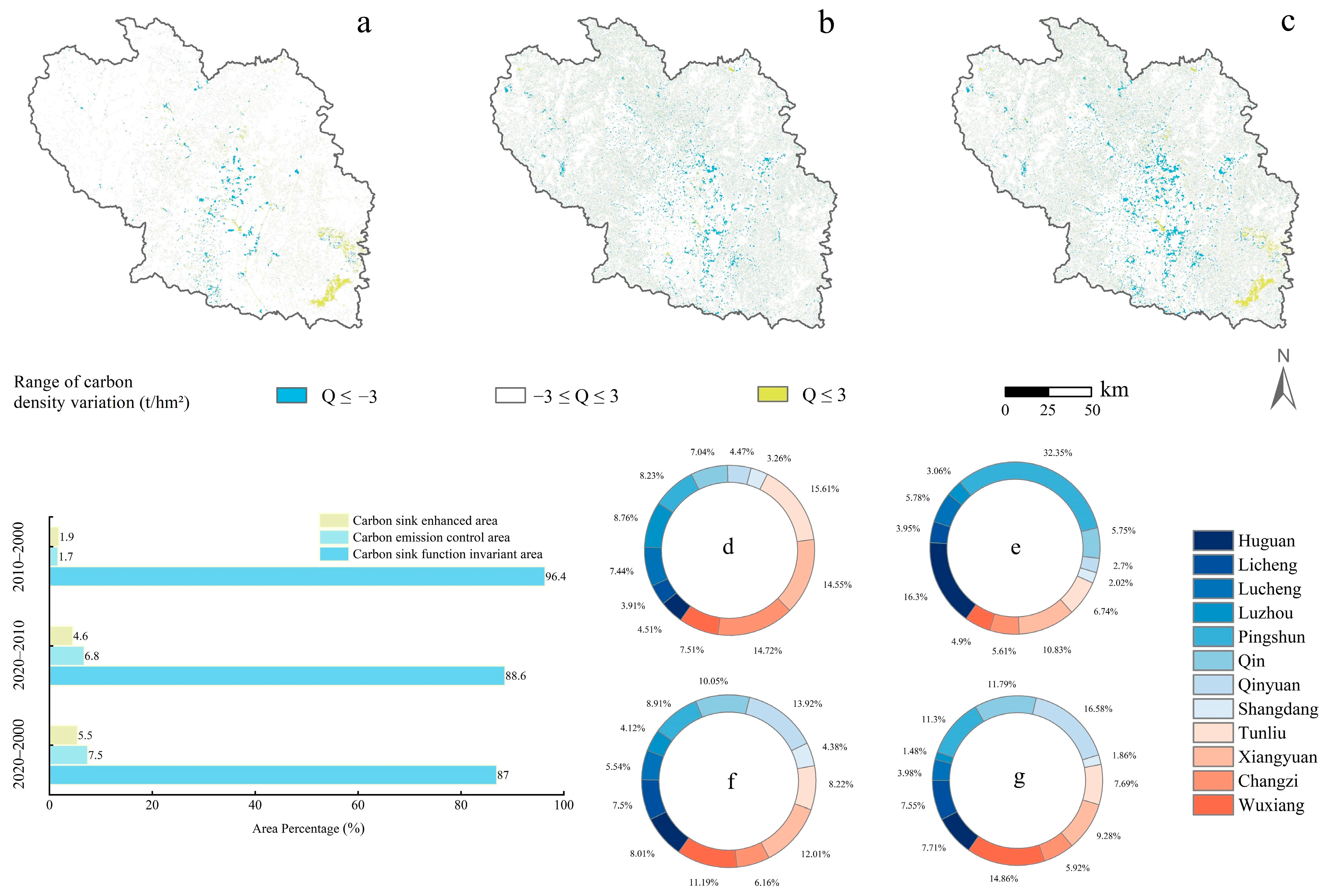
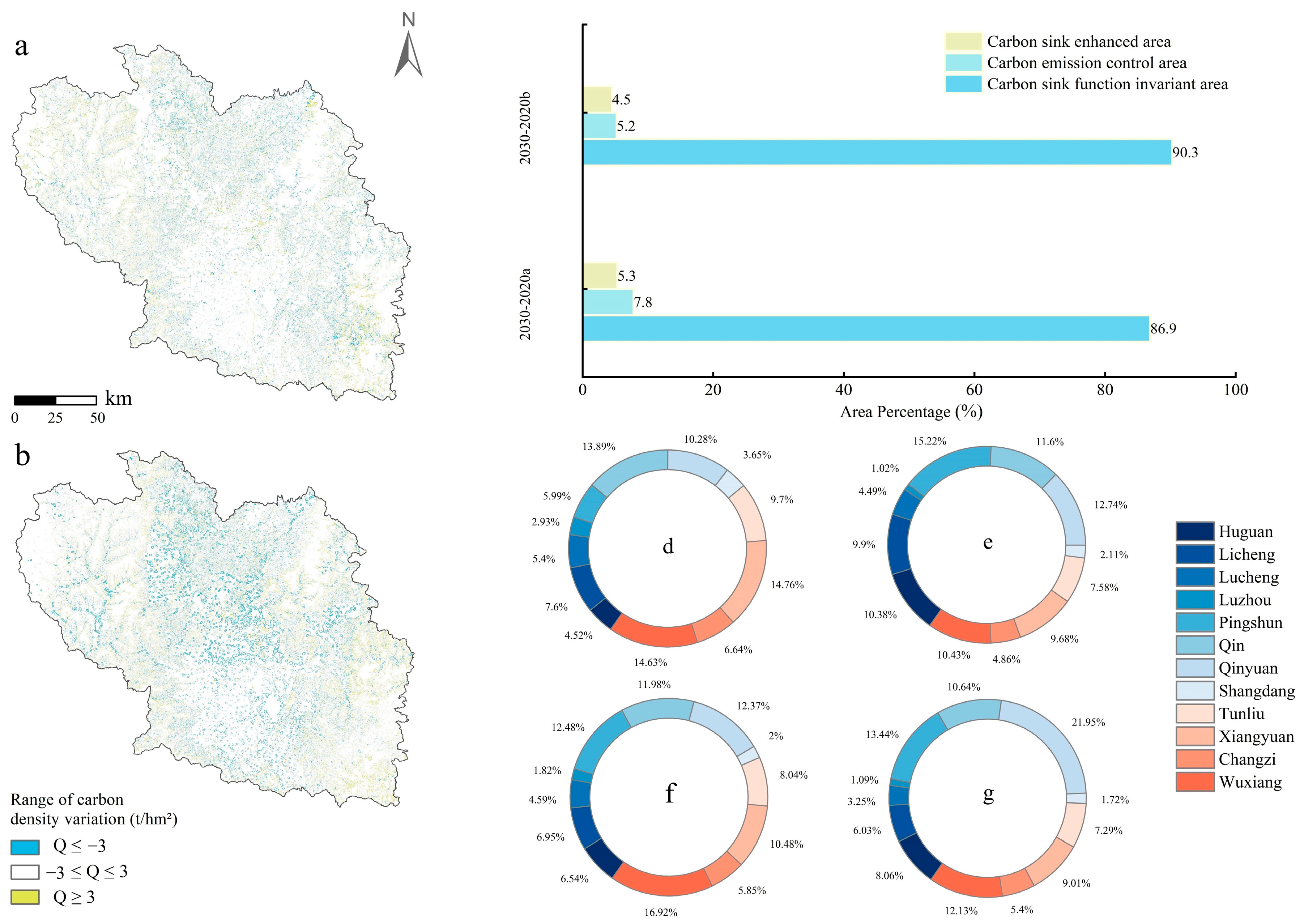
3.4.1. Division of Carbon Sink Functional Area

Referring to the existing results, combined with the actual carbon density changes in Changzhi City during the study period, from the perspective of “carbon source-carbon sink”, considering the impact of temperature, precipitation, and land-use type conversion on carbon density, the Changzhi City ecological system carbon functions are divided into three types. Carbon sink enhancement area (Q < −3 t/ha), carbon sink stabilization area (−3 t/ha ≤ Q ≤3 t/ha), carbon emission control area (Q < 3 t/ha), Q is Changes in carbon stocks [38,44] (Figure 9).

From 2000 to 2010, the proportion of carbon sink enhancement area was only 1.9%, mainly distributed in Huguan Taihang Mountain Grand Canyon National Geological Natural Park in the southeast of Changzhi City and Pingshun Tianji Mountain National Geological Park in the east. The dense distribution of ecological reserves and nature reserves in the region positively affects the reproduction and expansion of forests. The proportion of carbon emission control area was 1.7%, mainly concentrated in Tunliu District, Xiangyuan County, Changzi County, Lucheng District, Luzhou District, and Shangdang District in the central and southern parts of Changzhi City. These areas are mainly due to the rapid expansion of artificial surfaces, large-scale mining, forest land, grassland degradation, and loss of cultivated land. From 2010 to 2020, the proportion of carbon sink enhancement area was 4.6%, and the proportion of carbon emission control area was 6.8%, both of which were several times higher than the period from 2000 to 2010. The difference is that the enhanced carbon sink function distribution was more discrete this time. The carbon emission control area distribution is still relatively concentrated, mainly in Luzhou District, Shangdang District, Xiangyuan County, and Lucheng District in the central part of Changzhi City. From 2000 to 2020, the proportion of carbon emission control area was 7.5%, and the proportion of carbon sink enhancement area was 5.5%, and the spatial distribution was similar to that of 2010 to 2020. From 2000 to 2010, the areas with higher average carbon losses were Tunliu District and Xiangyuan County, where mean carbon density decreased by 0.42 t/ha and 0.40 t/ha, respectively. The highest mean carbon density increases were in Pinshun County and Huguan County, with increases of 2.64 t/ha and 2.32 t/ha, respectively. Pingshun County is also the area with the most significant increase in total carbon, increasing by 398,497.58 t. The most significant total carbon loss is in Tunliu District, with a loss of 47,046.39 t. From 2010 to 2020, Luzhou District had the highest average carbon loss, reaching 1.33 t/ha; Pingshun County had the highest average carbon increment, with a value of 0.62 t/ha; Xiangyuan County had the highest total carbon loss, with 72,492.22 t, and Qinyuan County had the highest carbon increment with a value of 103,561.22 t. From 2000 to 2020, Luzhou District had the highest average carbon loss with 1.39 t/ha, Pingshun County had the highest average carbon increment with 3.25 t/ha; Xiangyuan County had the highest total carbon loss with 119,538.61 t, and the highest carbon increment is in Pingshun County, with 491,456.17 t.

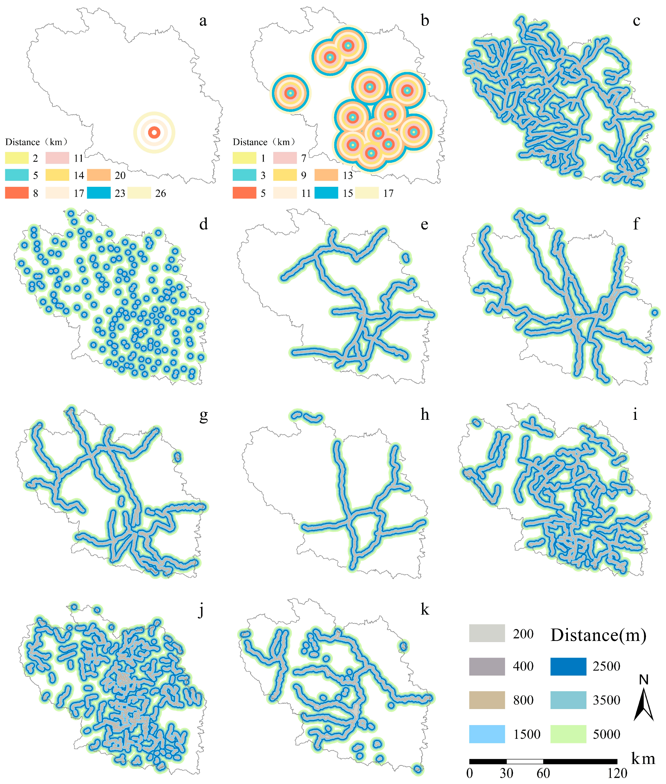
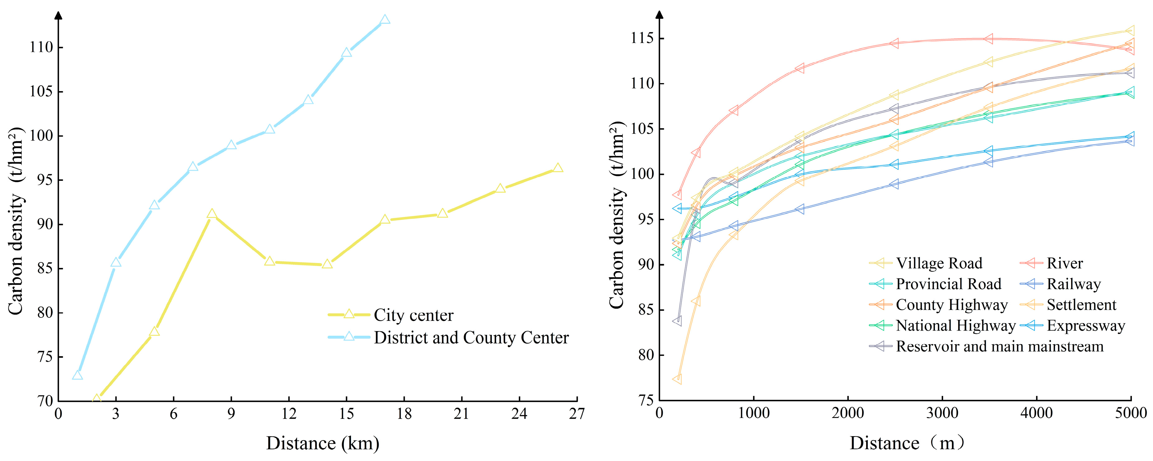
3.4.2. Buffer Analysis of Carbon Stocks

ArcGIS software was used to analyze the interrelationship between the distance between each influencing factor and the change in carbon stock density. According to the findings, carbon sequestration potential at various distances in Changzhi city center is significantly lower than in county centers, indicating a significant gap in carbon sequestration capacity (Figure 10 and Figure 11). Generally speaking, different distances in urban areas of different grades have different carbon sink effects. The carbon sink effect of county-level district areas is generally more significant than that of prefecture-level cities. Prefecture-level cities have a more significant carbon sink effect than provincial capital cities. The higher the level of the administrative center, the larger and more complex the scope of its carbon sink effect. The data show that regional carbon density increases with distance from Changzhi’s center, with a sharp increase from 70.17 t/ha to 91.13 t/ha in the 2–8 km range and a decrease followed by an increase in the 8–20 km range, with a slow increase beginning again after 20 km. This is because of a large area of water body (Zhangze reservoir) within 8–20 km, which has led to a significant decrease in carbon density. According to the carbon stock growth curve, the impact of Changzhi City’s urban area on carbon density occurs mainly within an 8 km radius of the urban area, which is consistent with the objective rule that the further away from the urban center, the greater the carbon density. The change in carbon stock density around the county center is also consistent with the rule that the higher the carbon density, the further away from the county center, and the growth rate is significantly faster than that of Changzhi city center, and the growth curve shows that the influence radius of the county center is approximately 7 km.

The effect of different road grades on carbon stock density is shown in Figure 11. Higher-level roads correlate more strongly with lower carbon density, and regional carbon stock density increases with increasing road distance. The data show that the carbon density within 200 m around the national road is the lowest at 91.70 t/ha, and within 200 m of the provincial road is 91.05 t/ha. The carbon density within 200 m of the township road, county road, and railway are 92.94 t/ha, 92.36 t/ha, and 92.73 t/ha. Expressway has the lowest carbon density within 200 m (96.22 t/ha), and provincial roads have a significant increase in carbon density within 800 m (an increase of 1.33 t/ha per 100 m) and only 0.24 t/ha per 100 m from 800 m to 5000 m. Increases of 0.72 t/ha per 100 m are evident within 1500 m of the national road; after 1500 m, the increase in carbon intensity plateaus at 0.22 t/ha per 100 m. The value tends to be stable within 400 m of the expressway, and the increase is more significant within 400–1500 m, with an increment of 0.34 t/ha per 100 m, and stabilizes after 1500 m, with an increment of 0.12 t/ha per 100 m. The carbon density of township and county roads increased significantly within 800 m, with increments of 1.21 t/ha and 1.25 t/ha per 100 m, respectively, and then stabilized with increments of 0.37 t/ha and 0.34 t/ha per 100 m after 800 m. There is no significant change in the increase near the railway, and the increase in carbon density within 200–5000 m is all relatively flat, with an increase of 0.23 t/ha per 100 m. County roads and township roads have carbon densities of 114.48 t/ha and 115.88 t/ha at 5000 m, respectively, and the total increase in carbon density from 200–5000 m is 22.12 t/ha and 22.93 t/ha, significantly higher than national roads, provincial roads, railways, and expressways. On provincial roads, the carbon density at 5000 m is 109.13 t/ha, increasing by 18.08 t/ha from 200 to 5000 m. On national roads, railways, and expressways, the carbon density at 5000 m is 108.94 t/ha, 103.66 t/ha, and 104.16 t/ha, respectively, with 17.24 t/ha, 10.93 t/ha, and 7.94 t/ha, in terms of distance. The variance in carbon stocks density of rivers, reservoirs, and settlements follows the law of increased carbon density as distance increases. Within 200 m of the river, the carbon density is as high as 97.73 t/ha, significantly exceeding the carbon density within 200 m of roads at all levels, settlements, Changzhi city center, county centers, and reservoirs, increasing to 113.74 t/ha at 5000 m, for a total increase of 16.01 t/ha. River carbon density increases rapidly in the 200–1500 m range, reaching 1.08 t/ha per 100 m increment; after 1500 m, the increase tends to plateau, and at 3500–5000 m, carbon density decreases slightly, with only −0.06 t/ha per 100 m increment. Within 200 m of reservoirs, the carbon density is 83.79 t/ha and increases most sharply between 200 and 800 m, reaching an increment of 2.55 t/ha per 100 m, with a sightly decrease between 800 and 1500 m, and then continues to increase slowly, reaching 111.19 t/ha at 5000 m, with an increment of 0.29 t/ha per 100 m between 800 and 5000 m. Within 200 m of the settlement, the carbon density is 77.37 t/ha, which is significantly lower than the carbon density within the same distance of roads, rivers, and reservoirs at all levels, and increases more significantly between 200 and 1500 m, with an increment of 1.69 t/ha per 100 m, and tends to level off between 1500 and 5000 m, with an increment of 0.35 t/ha per 100 m, and increases to 111.66 t/ha by 5000 m, an increase of 34.29 t/ha from 200 to 5000 m.

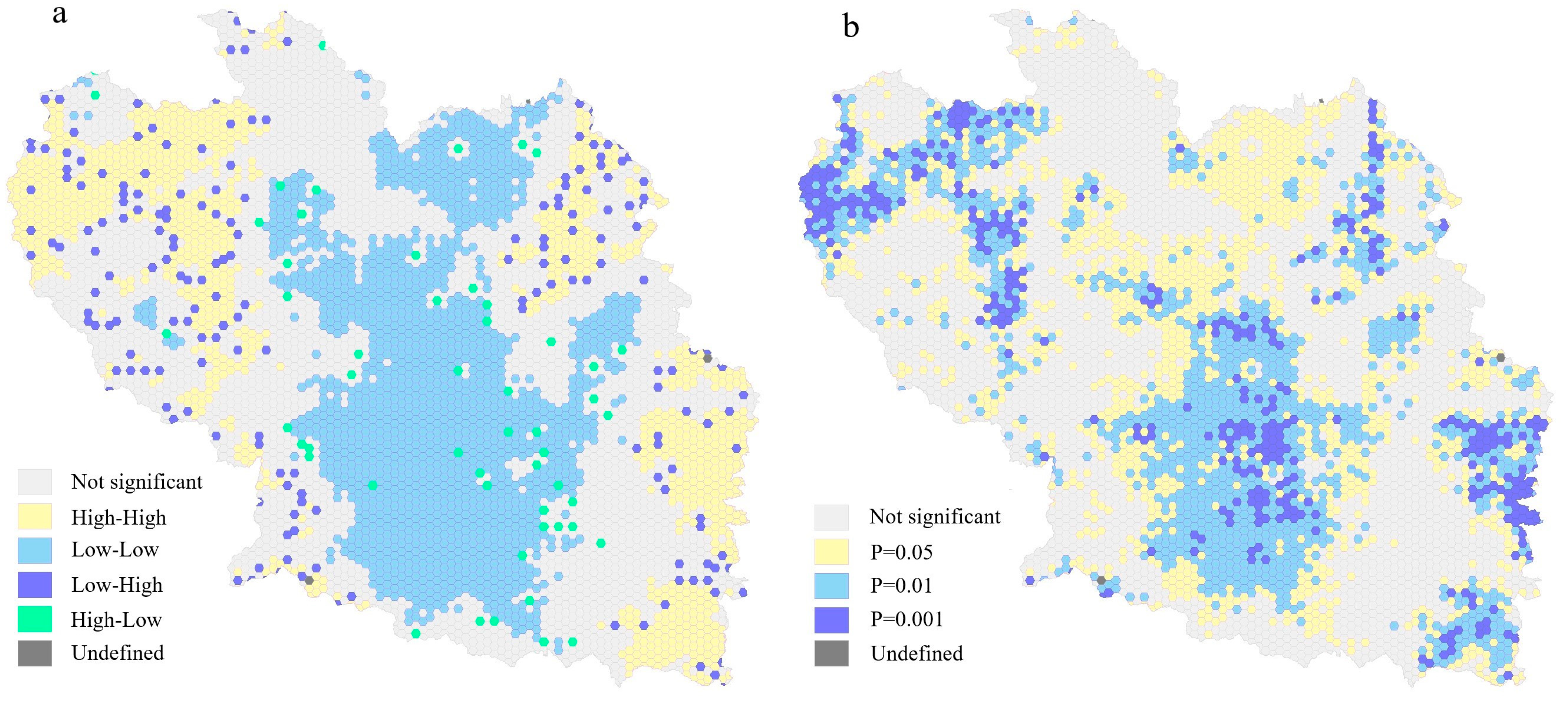
3.4.3. Spatial Autocorrelation Analysis

Using the Hexagon plug-in in GIS software, a hexagonal grid with a side length of 1 km was created for the study area. The grid was then used to perform zonal statistics and spatial autocorrelation analysis of carbon density in the study area. The results are depicted in Figure 12. Moran’s I showed that the global Moran’s I value was 0.587, which passed the 1% significance test. It shows a significant positive spatial correlation in the distribution of carbon density in Changzhi City, and there is a significant aggregation in the geographical spatial distribution. The aggregation types are shown in Figure 12a,b represents the confidence level, with smaller p-values representing the higher the confidence level. The high and high aggregations are mainly distributed on the east and west sides of Changzhi City, with Qinyuan County and the northern part of Qin County, the western part of Licheng County, and the eastern part of Huguan County and Pingshun County. Most of these areas are dominated by forest land, and there are many critical ecological lands such as national forest parks and nature reserves, which have an extremely high carbon storage capacity and have a positive radiation effect on the surrounding areas. The low-low agglomeration mainly occurs in the middle of Changzhi City. The main land types are mainly cultivated land and artificial surface, and the carbon storage density is low. The low-high aggregation is discrete around the high-high aggregation, and the distribution type is mainly grassland. The high-low aggregation is mostly discrete around the low-low aggregation, mostly in the junction of artificial surface and forest land or cultivated land and forest land, which is the area of steep change in carbon density.

3.4.4. Analysis of Carbon Stocks under the ND and CD Scenarios

Under the ND scenario (Figure 13), the carbon sink enhancement area proportion in 2030 is 5.3%. The distribution is still dominated by Pingshun and Huguan counties in the east and Qingyuan and Qin counties in the west, and the total amount of forest land carbon increased by 3,088,892.04 t (

Table 5. Changes in carbon stocks for each LULC class from 2020 to 2030.

LULC Types	LULC 2020 (a)	ND 2030 (b)		CD 2030 (c)
	Carbon Stock	Carbon Stock	b–a	Carbon Stock	c–a
Cultivated land	51,592,878.15	45,884,064.84	−5,708,813.31	49,993,680.12	−1,599,198.03
Forest land	70,229,893.63	73,318,785.67	3,088,892.04	71,919,101.80	1,689,208.17
Grassland	27,228,837.95	25,922,154.20	−1,306,683.75	26,718,771.65	−510,066.30
Water body	172,833.57	173,884.23	1050.66	179,662.86	6829.29
Artificial surface	5,160,443.26	9,150,504.70	3,990,061.44	6,030,136.30	869,693.04
Total	154,384,886.56	154,449,393.64	64,507.08	154,841,352.70	456,466.17

Results presented in raster images by pixels representing areas of 30 × 30 m; and converted into hectares by applying the Raster Calculator 11.1111111 for the conversion.

). The proportion of carbon emission control area is 7.8%, which is still concentrated in the central part of Changzhi City, but there is an evident trend of northward shift, with Wuxiang, Xiangyuan and Qin counties accounting for a significantly larger proportion. The loss of cultivated land is still the leading cause of carbon stock loss, and the total amount of carbon lost from cultivated land reaches −5,708,813.31 t. The area of carbon sink stabilization area accounts for 86.9%. The area of carbon emission control area under the CD scenario is reduced to 5.2%. The distribution pattern is also obviously changed, with Wuxiang County and Pingshun County accounting for the largest proportion, the effective protection of cultivated land is the main reason for the significant reduction in the area of carbon emission control area, and the total amount of carbon lost from cultivated land is reduced to −1,599,198.03 t. The area of carbon sink enhancement area is reduced to 4.5%, and the distribution is dominated by Qingyuan County and Pingshun County, and the growth of forest land is the primary source of carbon, and the growth amount is 1,689,208.17 t. The area of carbon sink stabilization accounts for 90.3%.

4. Discussions

4.1. Influence of Factors on Land-Use Change

Natural, social, and locational variables play an essential role in Changzhi’s land-use change. Ecological protection and land-use rules also significantly impact land-use change. The implementation of ecological conservation policies (such as the GFG program) is the main driver of reforestation and grass restoration, as previous scholars have concluded [45,46]. Due to the numerous effects of rapid urbanization and the policy of returning farmland to forest and grass, Changzhi’s cultivated land has been declining for the past 20 years. Although the implementation of the cultivated land protection system has slowed the loss of cultivated land to some degree, particularly with the implementation of the policy to balance the occupation of cultivated land in part of the last decade, the loss of cultivated land and the expansion of artificial surface caused by rapid urbanization still cannot be prevented [47,48]. During the 20 years, only the cultivated land area in Pingshun County increased, and the growth ratio and area in the first 10 years reached 3.48% and 12.58 km², respectively. This is primarily due to the deterioration of the grassland ecosystem environment and the implementation of the ecological protection policy of returning farmland to grassland in Pingshun County, where the grassland area decreased by 64.22 km² from 2000 to 2010. In the first 10 years, the cultivated land area decreased the most in Changzi County. The largest proportion was reduced in Luzhou District; in the later 10 years, Xiangyuan County decreased the most, and Luzhou District remained the largest proportion. These are the critical mineral resource distribution areas in Changzhi City, and urban expansion and mine mining occupy and destroy a large amount of cultivated land. The impacts of opencast mining will directly change land-use types and surface landscapes in the short term, for example by reducing forests and grasslands and increasing other lands. Underground mining will lead to geological hazards such as ground fissures and collapse pits and will result in a reduction in agricultural land and water bodies and an increase in other types of land [49]. Over the last 20 years, the area of forest land has steadily increased, with national policies such as reverting farming to forest and afforestation playing a crucial part in this. The results of Zhang et al. [50] showed that ecological engineering with the Grain to Green Program (GTGP) significantly contributed to carbon sequestration in the soils of China by converting farmland to forestland. The results of Lu et al. [51] showed that ecological engineering contributed 56% to the regional carbon stock in China as the area of forestland and grassland increased.

With nature reserves such as the Shanxi Mianshan Provincial Nature Reserve, the Tianji Mountain National Geological Park, Xigou Forest Park within their borders, and nature conservation policies, Qingyuan County and Pingshun County on both sides of Changzhi City are the critical areas of forest land growth and distribution. On the other hand, Qingyuan and Pingshun counties have undulating peaks and largely mountainous terrain, with high altitudes and slopes limiting cultivated land development while promoting the conversion of cultivated land to forest land. The effect of slopes on the return of cultivation to forests in Changzhi is even more significant. This is closely related to China’s policy of implementing fallowing on farmland with slopes greater than 25 degrees since 1999 [52]. The conversion of grassland to cultivated land may be due to increased temperature and precipitation in northern China due to global warming over the past two decades, which has pushed the boundaries of cultivated land northwards and facilitated the reclamation of barren grassland into cultivated land. Wang et al. [53] and Xin and Li et al. [54] argue that increased precipitation and temperature in northern China, as well as the northward shift in the boundary of land suitable for cultivation, have facilitated the reclamation of barren grasslands and unused land in the north, leading to an increase in the area of cultivated land. In addition to this, there may be a lack of clarity in grassland tenures, such as the classification of certain grassland as shrubland and open forestland, which could be one of the reasons for the changes in grassland, which could also explain the grassland logistic regression analysis’ lower ROC values. Over 20 years, the wetland area has grown steadily. In the first decade, the wetlands were primarily located within the Shanxi Qianquan Lake National Wetland Nature Park and near the Zhangze Reservoir in the second. This has been made possible by the national implementation of the Wetland Protection Programme (WPP), which facilitated the conversion of land-use/cover types to forestlands and wetlands [55]. The Changzhi National Urban Wetland Park Plan, launched in 2008 and divides the Zhangze Reservoir and the surrounding 80 km² area into priority conservation and planning areas, is the main reason for the steady increase in wetland areas and the shift in focus.

4.2. Influence of Factors on Ecosystem Carbon Stocks

Changzhi’s carbon stock increased by 680,989.73 t between 2000 and 2020, and the area of carbon sink enhancement area from 2010 to 2020 is 313% of that from 2000 to 2010. The improvement of the carbon sink is attributed to the implementation of several ecological projects in Changzhi, such as the Changzhi City Grain for Green Project, which has produced impressive results since its inception in 2002. By the beginning of 2020, the city had completed the previous round of reforestation and the news cycle, totaling 1027.1 km², with 304.7 km² of reforestation and 722.4 km² of barren hill afforestation. The main reason for Changzhi’s increased carbon storage is conversing cultivated land to forest land. Changzhi is undergoing a period of rapid urbanization. The conversion of cultivated land and natural land to artificial surface is the main reason for the loss of carbon stocks in Changzhi. The extremely rapid expansion of artificial surface is a problem that needs to be addressed for Changzhi’s coordinated development. Limiting the remarkably rapid expansion of artificial surface to cultivated and natural ecological land is critical for the carbon sink effect in Changzhi and collaborative urban and rural development. In contrast to the anthropogenic conversion of forest and cultivated land to artificial surface, another evident land transformation is grassland degradation, which is primarily dependent on environmental degradation. Shanxi Province has a dry climate and a vulnerable biological environment. It is one of the most severe grassland degraded regions in northern China, with 95% of the province’s total grassland area degraded and 30% completely lost to use. Degradation of grassland emits carbon directly and results in the expansion of unused land, accelerating regional warming and increasing evaporation, creating a vicious cycle of carbon stock loss. As a result, land development in northern and northwestern China must be strictly regulated, as inappropriate land-use policies could deteriorate the fragile ecological environment. The more delicate the area is, the more development-friendly land policies should be enforced.

4.3. Impact of Spatial Geographic Location on Carbon Stocks

With distance from the city center, carbon stock density increases. The central area of a city is generally a multi-functional agglomeration of the city’s political, economic, social, cultural, and religious aspects, as well as the area with the strongest historical deposits and the densest distribution of building land, which has a strong economic radiation effect on the surrounding areas. The density of built land begins to decline as the distance from the administrative center increases, and land-use types such as cultivated land, grassland, forest, and other natural lands gradually emerge, as well as scenic spots, nature reserves, etc. These areas are distributed as urban ecological barriers on the city’s periphery, which explains why the density of carbon storage increases as the distance from the city center increases. On the other hand, the more senior administrative centers have more complex carbon stock changes. Although the carbon density of Changzhi city center is much less than that of county centers, the scope of influence is greater. This is due to the difference in land-use structure and urban spatial layout between the city and the county center [56]. The better grades centers are more modernized and have a denser distribution of built-up land and a wider radiation range. Moreover, carbon storage fluctuated significantly between 8 and 16 km from the city center, which is attributed to the Zhangze Reservoir influencing the average carbon density of nearby land types. For roads, it is a common feature that the density of carbon stocks increases with distance, but there are some differences in the influence of different classes of roads. More lanes and faster traffic speeds lead to increased traffic flows. Vehicle exhaust and other forms of air pollution have been shown to harm the carbon sink of regional ecosystems. Different levels of roads have different impacts on surrounding land-use changes, which explains why the density of carbon storage near national and provincial roads is significantly lower than that near township and county roads [57]. The higher carbon density near rivers is due to the abundant water resources for vegetation growth near rivers. In contrast, the carbon density of reservoirs fluctuates between 400–800 m because the Zhangze reservoir is located near the urban center, where there is a large concentration of built-up land, causing a slight decrease in carbon density, which is also the reason for the lower mean carbon density near the settlements.

4.4. LUCC and Carbon Stock Changes in 2030

Under the ND scenario, the primary land-use type shifts during 2020–2030 are cultivated land conversion to forest land, grassland, and construction land, with cultivated land to forest land dominating. This continues the probability of land-use transfer from 2010 to 2020, especially the occupation of cultivated land by construction land expansion. The conversion of cultivated land to construction land is the main form of carbon loss and the reason for the expansion of the area of carbon emission control area. This situation is well curbed under the CD scenario. The carbon emission control area in the central part of Changzhi City is significantly reduced due to the delineation of the basic farmland protection zone, which plays a good role in protecting the cultivated land area and reduces the loss of carbon stock in Changzhi City to a certain extent. The conversion of cultivated land to forest land becomes mainstream under the CD scenario, At the same time, the transfer out of forest land is also reduced due to the ecological and nature protection zones. The increase in forest land area is an essential source of carbon stock increase, and most of the enhanced carbon sink areas in the east and west of Changzhi City come from this. Grassland area decreases in both scenarios, and the decrease is more significant in the ND scenario. Ecological reserves and nature reserves do not prevent the decrease of grassland area but reduce the decrease rate to some extent. The different land-use patterns under the two scenarios indicate that the designation of basic farmland and protected areas has played a good role in protecting the carbon stock in Changzhi City.

4.5. Uncertainties

The InVEST model focuses on carbon stock changes among different land-use types when calculating carbon stocks and will ignore the effects within vegetation and soil and the differences in carbon sequestration functions brought by spatial heterogeneity and different age structures of vegetation. In addition, this study determined the carbon density values of land-use types by referring to existing research data for correction and did not conduct field surveys on carbon density in Changzhi, which inevitably had some errors with the actual values. Future studies should focus on combining field research and calculation models to improve the accuracy of carbon stock estimation. The application of the CA-Markov composite model overcomes the drawbacks of a single model and realizes the dual optimization of quantitative simulation and spatial location simulation. Although the model in this experiment takes local policies (red line of basic farmland protection, ecological reserve, and nature reserve) into account, it does not fully consider the city’s future planning and development direction. Future research should fully integrate regional policies and urban development planning to improve the scientific foresight and the rationality of decision-making. The hexagonal grid size was used as a fixed value when using the spatial autocorrelation model for analysis. Although the correlation met the standard, the scale effect was not fully considered. Conducting research at multiple scales to minimize the influence of scale effects is the direction we need to work on in the future.

5. Conclusions

Based on the Clue-S model and the binary logistic regression model, this study reveals the evolution of land-use change in Changzhi City, analyzes the drivers of land-use change, and uses the CA-Markov model and the InVEST model to simulate future land-use scenarios and analyze the spatial pattern of carbon storage in Changzhi City. The findings show that land-use patterns and types in Changzhi have changed significantly over the last 20 years. From 2000 to 2020, the area of cultivated land in Changzhi decreased by 327.19 km² while artificial surface area increased by 382.01 km², with over 90% of the expansion of artificial surface coming from the occupation of cultivated land. Artificial surface’s growth rate far outpaces other land types, with low elevation, gentle slope, population growth, and economic development driving the conversion of cultivated land into artificial surface. Forest expanded by 70.78 km² while grassland shrank by 143.91 km², with topographic and geographical differences significant in both changes. The conversion of each land type is influenced by transport accessibility, but they are not decisive. Land-use management policies and the plan to return farmland to forests have helped protect farmland and natural land to some extent, but they have not changed the fact that artificial surface area is expanding rapidly. The main reason for the decline in carbon stocks is the loss of large cultivated land areas. In contrast, the expansion of forest and wetland areas is the primary source of carbon stock growth, thanks to the implementation of a series of ecological policies such as the return of farmland to forest and the wetland national park plan. At the same time, the average annual precipitation in Changzhi has increased, and the temperature has stabilized over the past 20 years, so there has been an overall trend of increasing carbon stocks.

The total carbon stock in Changzhi City increased by 542,708.62 t in the first 10 years, with the carbon sink function enhancement area accounting for 1.9%, concentrated in Huguan and Pingshun counties, and the carbon loss area accounting for 1.7%, concentrated in the central part of Changzhi City. The total carbon stock increased by 83,811.95 t in the last decade, with the carbon sink function enhancement area accounting for 4.6%, which is more discrete. The carbon loss area accounted for 6.8%, still concentrated in the central area. Further analysis of the spatial distribution of carbon stocks in 2020 reveals that urban centers, roads at all levels, rivers, and reservoirs significantly impact the density of carbon stocks in the neighborhood. Carbon stock density rises with distance from urban centers, all-level roads, rivers, and reservoirs; carbon stock density around district and county centers is higher than that around urban centers, and carbon stock density around high-grade roads is lower than that of low-grade roads, related to the traffic flow on each level road. The density of building sites causes the lowest carbon density around settlements.

Under the ND and CD scenarios, the land-use pattern of Changzhi City 2030 changes significantly, with a large area of cultivated land transformed into artificial surface and grassland transformed into forest land under the ND scenario, and the area of carbon emission control area and carbon sink enhancement area is 7.8% and 5.2%, respectively. Under the CD scenario, the area of cultivated land and grassland shows a slight decrease due to the protective effect of the red line zone, and the growth of artificial surface is thus limited, and the area of carbon emission control area and carbon sink enhancement area decreases to 5.3% and 4.5%, respectively. The total carbon stock of the CD scenario is 392,011.85 t higher than the ND scenario and 456,466.17 t higher than 2020.

Therefore, more attention should be paid to these areas in future ecological restoration and urban expansion. The carbon sink enhancement areas should be protected to prevent them from being converted from a carbon sink to a carbon source. The carbon emission control areas should be repaired as much as possible to convert them from a carbon source to a carbon sink. Establishing an accurate regional carbon density database is also imperative for assessing regional terrestrial ecosystems. Precise and detailed research on regional carbon density data, combined with remote sensing data can monitor regional terrestrial ecosystem carbon stocks in real time, accurately quantify the contribution of a series of ecological projects and land reclamation and restoration to regional carbon sinks, build a reasonable urban expansion pattern based on the spatial and temporal distribution of carbon stocks, and explore scientific development patterns in the context of carbon peaking and carbon neutrality goals. In a word, we should study the problems, find out the problems, and adjust the policies in time through scientific methods. Focusing on the protection of ecologically fragile areas, strengthening the restoration of ecologically degraded areas, and constructing a reasonable urban expansion pattern are all important components of achieving the carbon peaking and carbon neutrality goals through the path of carbon protection and carbon sink increase.

References

1. Wang, L.; Ma, D.; Chen, W. Future CO2 Emissions Allowances and Inequality Assessment under Different Allocation Regimes. Energy Procedia. 2014, 61, 523–526. [Google Scholar] [CrossRef] [Green Version]
2. Houghton, R.A. Revised estimates of the annual net flux of carbon to the atmosphere from changes in land use and land management 1850–2000. Tellus Ser. B Chem. Phys. Meteorol. 2003, 55, 378–390. [Google Scholar] [CrossRef] [Green Version]
3. Kleinen, T.; Gromov, S.; Steil, B.; Brovkin, V. Atmospheric methane underestimated in future climate projections. Environ. Res. Lett. 2021, 16, 094006. [Google Scholar] [CrossRef]
4. Friedlingstein, P.; O’Sullivan, M.; Jones, M.W.; Andrew, R.M.; Hauck, J.; Olsen, A.; Peters, G.P.; Peters, W.; Pongratz, J.; Sitch, S.; et al. Global Carbon Budget 2020. Earth Syst. Sci. Data 2020, 12, 3269–3340. [Google Scholar] [CrossRef]
5. Le Quéré, C.; Raupach, M.R.; Canadell, J.; Marland, G.; Bopp, L.; Ciais, P.; Conway, T.J.; Doney, S.; Feely, R.A.; Foster, P.; et al. Trends in the sources and sinks of carbon dioxide. Nat. Geosci. 2009, 2, 831–836. [Google Scholar] [CrossRef]
6. Luyssaert, S.; Schulze, E.-D.; Börner, A.; Knohl, A.; Hessenmöller, D.; Law, B.; Ciais, P.; Grace, J. Old-growth forests as global carbon sinks. Nature 2008, 455, 213–215. [Google Scholar] [CrossRef] [PubMed]
7. Xu, H.; Song, Y.; Tian, Y. Simulation of land-use pattern evolution in hilly mountainous areas of North China: A case study in Jincheng. Land Use Policy 2022, 112, 105826. [Google Scholar] [CrossRef]
8. Geist, H.J.; Lambin, E.F. Proximate Causes and Underlying Driving Forces of Tropical Deforestation. Bioscience 2002, 52, 143–150. [Google Scholar] [CrossRef]
9. Fang, S.; Gertner, G.Z.; Sun, Z.; Anderson, A.A. The impact of interactions in spatial simulation of the dynamics of urban sprawl. Landsc. Urban Plan. 2005, 73, 294–306. [Google Scholar] [CrossRef]
10. Glp, G. Science Plan and Implementation Strategy. Environ. Policy Collect. 2009, 20, 1262–1268. [Google Scholar]
11. Tang, F.; Fu, M.; Wang, L.; Zhang, P. Land-use change in Changli County, China: Predicting its spatio-temporal evolution in habitat quality. Ecol. Indic. 2020, 117, 106719. [Google Scholar] [CrossRef]
12. Clerici, N.; Cote-Navarro, F.; Escobedo, F.J.; Rubiano, K.; Villegas, J.C. Spatio-temporal and cumulative effects of land use-land cover and climate change on two ecosystem services in the Colombian Andes. Sci. Total Environ. 2019, 685, 1181–1192. [Google Scholar] [CrossRef]
13. Yu, B.; Yang, L.; Chen, F. Semantic Segmentation for High Spatial Resolution Remote Sensing Images Based on Convolution Neural Network and Pyramid Pooling Module. IEEE J. Sel. Top. Appl. Earth Obs. Remote Sens. 2018, 11, 3252–3261. [Google Scholar] [CrossRef]
14. Anputhas, M.; Janmaat, J.J.A.; Nichol, C.F.; Wei, X.A. Modelling spatial association in pattern based land use simulation models. J. Environ. Manag. 2016, 181, 465–476. [Google Scholar] [CrossRef]
15. Han, J.; Hayashi, Y.; Cao, X.; Imura, H. Application of an integrated system dynamics and cellular automata model for urban growth assessment: A case study of Shanghai, China. Landsc. Urban Plan. 2009, 91, 133–141. [Google Scholar] [CrossRef]
16. Aburas, M.M.; Ho, Y.M.; Ramli, M.F.; Ash’Aari, Z.H. Improving the capability of an integrated CA-Markov model to simulate spatio-temporal urban growth trends using an Analytical Hierarchy Process and Frequency Ratio. Int. J. Appl. Earth Obs. Geoinf. 2017, 59, 65–78. [Google Scholar] [CrossRef]
17. Mas, J.-F.; Kolb, M.; Paegelow, M.; Olmedo, M.T.C.; Houet, T. Inductive pattern-based land use/cover change models: A comparison of four software packages. Environ. Model. Softw. 2014, 51, 94–111. [Google Scholar] [CrossRef] [Green Version]
18. Piao, S.; He, Y.; Wang, X.; Chen, F. Estimation of China’s terrestrial ecosystem carbon sink: Methods, progress and prospects. Sci. China Earth Sci. 2022, 65, 641–651. [Google Scholar] [CrossRef]
19. Piao, S.; Fang, J.; Ciais, P.; Peylin, P.; Huang, Y.; Sitch, S.; Wang, T. The carbon balance of terrestrial ecosystems in China. Nature 2009, 458, 1009–1013. [Google Scholar] [CrossRef]
20. Fang, J.; Chen, A.; Peng, C.; Zhao, S.; Ci, L. Changes in Forest Biomass Carbon Storage in China Between 1949 and 1998. Science 2001, 292, 2320–2322. [Google Scholar] [CrossRef]
21. Zhang, C.; Brodylo, D.; Sirianni, M.J.; Li, T.; Comas, X.; Douglas, T.A.; Starr, G. Mapping CO2 fluxes of cypress swamp and marshes in the Greater Everglades using eddy covariance measurements and Landsat data. Remote Sens. Environ. 2021, 262, 112523. [Google Scholar] [CrossRef]
22. Papale, D.; Reichstein, M.; Aubinet, M.; Canfora, E.; Bernhofer, C.; Kutsch, W.; Longdoz, B.; Rambal, S.; Valentini, R.; Vesala, T.; et al. Towards a more harmonized processing of eddy covariance CO2 fluxes: Algorithms and uncertainty estimation. Biogeosci. Discuss. 2006, 3, 961–992. [Google Scholar]
23. Gurney, K.R.; Law, R.; Denning, S.; Rayner, P.; Baker, D.; Bousquet, P.; Bruhwiler, L.; Chen, Y.-H.; Ciais, P.; Fan, S.; et al. Towards robust regional estimates of CO2 sources and sinks using atmospheric transport models. Nature 2002, 415, 626–630. [Google Scholar] [CrossRef] [Green Version]
24. He, C.; Zhang, D.; Huang, Q.; Zhao, Y. Assessing the potential impacts of urban expansion on regional carbon storage by linking the LUSD-urban and InVEST models. Environ. Model. Softw. 2016, 75, 44–58. [Google Scholar] [CrossRef]
25. Tallis, H.; Ricketts, T.; Guerry, A.; Sharp, R.; Wood, S.; Chaplin-Kramer, R.; Vogl, A.; Johnson, J.; Hamel, P.; Kennedy, C.; et al. InVEST 2.5.6 User’s Guide; The Natural Capital Project: Stanford, CA, USA, 2013. [Google Scholar]
26. Fernandes, M.M.; Fernandes, M.R.D.M.; Garcia, J.R.; Matricardi, E.A.T.; de Almeida, A.Q.; Pinto, A.S.; Menezes, R.S.C.; Silva, A.D.J.; Lima, A.H.D.S. Assessment of land use and land cover changes and valuation of carbon stocks in the Sergipe semiarid region, Brazil: 1992–2030. Land Use Policy 2020, 99, 104795. [Google Scholar] [CrossRef]
27. Zhang, Y.; Shi, X.; Tang, Q. Carbon storage assessment in the upper reaches of the Fenhe River under different land use scenarios. Acta Ecol. Sin. 2021, 41, 360–373. [Google Scholar] [CrossRef]
28. Huang, Y.; Tian, F.; Wang, Y.; Wang, M.; Hu, Z. Effect of coal mining on vegetation disturbance and associated carbon loss. Environ. Earth Sci. 2015, 73, 2329–2342. [Google Scholar] [CrossRef]
29. Hou, H.; Zhang, S.; Ding, Z.; Huang, A.; Tian, Y. Spatiotemporal dynamics of carbon storage in terrestrial ecosystem vegetation in the Xuzhou coal mining area, China. Environ. Earth Sci. 2015, 74, 1657–1669. [Google Scholar] [CrossRef]
30. MacDonald, K.I.; Corson, C. ‘TEEB Begins Now’: A Virtual Moment in the Production of Natural Capital. Dev. Change 2012, 43, 159–184. [Google Scholar] [CrossRef]
31. Pontius, R.; Schneider, L.C. Land-cover change model validation by an ROC method for the Ipswich watershed, Massachusetts, USA. Agric. Ecosyst. Environ. 2001, 85, 239–248. [Google Scholar] [CrossRef]
32. Sang, L.; Zhang, C.; Yang, J.; Zhu, D.; Yun, W. Simulation of land use spatial pattern of towns and villages based on CA–Markov model. Math. Comput. Model. 2011, 54, 938–943. [Google Scholar] [CrossRef]
33. Zhao, M.; He, Z.; Du, J.; Chen, L.; Lin, P.; Fang, S. Assessing the effects of ecological engineering on carbon storage by linking the CA-Markov and InVEST models. Ecol. Indic. 2019, 98, 29–38. [Google Scholar] [CrossRef]
34. Tang, X.; Zhao, X.; Bai, Y.; Tang, Z.; Wang, W.; Zhao, Y.; Wan, H.; Xie, Z.; Shi, X.; Wu, B.; et al. Carbon pools in China & rsquo; s terrestrial ecosystems: New estimates based on an intensive field survey. Proc. Natl. Acad. Sci. USA 2018, 115, 4021–4026. [Google Scholar] [CrossRef] [Green Version]
35. Xie, X. Organic Carbon Density and Storage in Soils of China and Spatial analysis. Acta Pedol. Sin. 2004, 41, 35–43. [Google Scholar]
36. Li, K.; Wang, S.; Cao, M. Vegetation and soil carbon storage in China. Sci. China Ser. D Earth Sci. 2004, 47, 49–57. [Google Scholar] [CrossRef]
37. Alam, S.; Starr, M.; Clark, B. Tree biomass and soil organic carbon densities across the Sudanese woodland savannah: A regional carbon sequestration study. J. Arid Environ. 2013, 89, 67–76. [Google Scholar] [CrossRef]
38. Zhou, J.; Zhao, Y.; Huang, P.; Zhao, X.; Feng, W.; Li, Q.; Xue, D.; Dou, J.; Shi, W.; Wei, W.; et al. Impacts of ecological restoration projects on the ecosystem carbon storage of inland river basin in arid area, China. Ecol. Indic. 2020, 118, 106803. [Google Scholar] [CrossRef]
39. Shoman, W.; Alganci, U.; Demirel, H. A comparative analysis of gridding systems for point-based land cover/use analysis. Geocarto Int. 2019, 34, 867–886. [Google Scholar] [CrossRef]
40. Birch, C.P.; Oom, S.P.; Beecham, J.A. Rectangular and hexagonal grids used for observation, experiment and simulation in ecology. Ecol. Model. 2007, 206, 347–359. [Google Scholar] [CrossRef]
41. Liu, K.; Yuan, F.; Pan, K. Evolution Analysis of Different Ownership Enterprises Spatial Organization Network in the Yangtze River Delta. Sci. Geogr. Sin. 2017, 37, 651–660. [Google Scholar]
42. Pike, K.; Wright, P. Protection through Valuation: Using Q Methodology to Explore the Intangible Benefits of a UK MPA. In Proceedings of the Global Congress on Integrated Coastal Management (ICM)—Lessons Learned to Address New Challenges, Marmaris, Turkey, 30 October–3 November 2013. [Google Scholar]
43. Keshtkar, H.; Voigt, W. A spatiotemporal analysis of landscape change using an integrated Markov chain and cellular automata models. Modeling Earth Syst. Environ. 2016, 2, 10. [Google Scholar] [CrossRef] [Green Version]
44. Wang, X.; Lu, F.; Qin, Y.; Sun, Y. Spatial and temporal changes of carbon sources and sinks in Henan Province. Prog. Geogr. 2016, 35, 941–951. [Google Scholar]
45. Long, H.; Tang, G.; Li, X.; Heilig, G.K. Socio-economic driving forces of land-use change in Kunshan, the Yangtze River Delta economic area of China. J. Environ. Manag. 2007, 83, 351–364. [Google Scholar] [CrossRef] [PubMed]
46. Wang, J.; Chen, Y.; Shao, X.; Zhang, Y.; Cao, Y. Land-use changes and policy dimension driving forces in China: Present, trend and future. Land Use Policy 2012, 29, 737–749. [Google Scholar] [CrossRef]
47. Zhou, Y.; Li, X.; Liu, Y. Rural land system reforms in China: History, issues, measures and prospects. Land Use Policy 2019, 91, 104330. [Google Scholar] [CrossRef]
48. Long, H.; Li, Y.; Liu, Y.; Woods, M.; Zou, J. Accelerated restructuring in rural China fueled by ‘increasing vs. decreasing balance’ land-use policy for dealing with hollowed villages. Land Use Policy 2012, 29, 11–22. [Google Scholar] [CrossRef]
49. Niu, Y.F.; Zhang, H.S.; Han-Xun, X.U. Research of Land Destruction Condition and Trend Caused by Underground Coal Mining in Changzhi. Coal Technol. 2016, 35, 305–307. [Google Scholar] [CrossRef]
50. Zhang, K.; Dang, H.; Tan, S.; Cheng, X.; Zhang, Q. Change in soil organic carbon following the ‘Grain-for-Green’ programme in China. Land Degrad. Dev. 2010, 21, 13–23. [Google Scholar] [CrossRef]
51. Lu, F.; Hu, H.; Sun, W.; Zhu, J.; Liu, G.; Zhou, W.; Zhang, Q.; Shi, P.; Liu, X.; Wu, X.; et al. Effects of national ecological restoration projects on carbon sequestration in China from 2001 to 2010. Proc. Natl. Acad. Sci. USA 2018, 115, 4039–4044. [Google Scholar] [CrossRef] [Green Version]
52. Deng, L.; Liu, S.; Kim, D.G.; Peng, C.; Sweeney, S.; Shangguan, Z. Past and future carbon sequestration benefits of China’s grain for green program. Glob. Environ. Change 2017, 47, 13–20. [Google Scholar] [CrossRef]
53. Wang, J.; Zhang, Z.; Liu, Y. Spatial shifts in grain production increases in China and implications for food security. Land Use Policy 2018, 74, 204–213. [Google Scholar] [CrossRef]
54. Xin, L.; Li, X. China should not massively reclaim new farmland. Land Use Policy 2018, 72, 12–15. [Google Scholar] [CrossRef]
55. Liu, J.; Li, S.; Ouyang, Z.; Tam, C.; Chen, X. Ecological and socioeconomic effects of China’s policies for ecosystem services. Proc. Natl. Acad. Sci. USA 2008, 105, 9477–9482. [Google Scholar] [CrossRef] [Green Version]
56. Xu, Q.; Dong, Y.-X.; Yang, R. Influence of the geographic proximity of city features on the spatial variation of urban carbon sinks: A case study on the Pearl River Delta. Environ. Pollut. 2018, 243, 354–363. [Google Scholar] [CrossRef] [PubMed]
57. Zhang, W.; Huang, B.; Luo, D. Effects of land use and transportation on carbon sources and carbon sinks: A case study in Shenzhen, China. Landsc. Urban Plan. 2014, 122, 175–185. [Google Scholar] [CrossRef]
Figure 1. Methodological framework applied for simulating current and future carbon stocks of Changzhi city in Shanxi, China.
Land 11 01270 g001
Figure 2. Study site location of Changzhi city in Shanxi, China.
Land 11 01270 g002
Figure 3. Land use and land cover (LULC) in 2000 (a), 2010 (b), 2020 (c) in Changzhi City.
Land 11 01270 g003
Figure 4. Land use and land cover (LULC) dynamics between 2000 and 2020 in Changzhi City.
Land 11 01270 g004
Figure 5. LUCC in Changzhi City between 2000–2010 (a), 2010–2020 (b) [42].
Land 11 01270 g005
Figure 6. Mining area, basic farmland protection zone, ecological protection zone, nature reserve, geological disaster site, coal mining sinkhole of Changzhi.
Land 11 01270 g006
Figure 7. LUCC in mining areas of Changzhi City between 2000–2020.
Land 11 01270 g007
Figure 8. Observed (a) and simulated (b) land use and land cover (LULC) in 2020, natural development (c) and conservation development (d) land use and land cover (LULC) in 2030.
Land 11 01270 g008
Figure 9. Spatial distribution of carbon density and carbon function areas in Changzi County from 2000 to 2020. (ac) are the carbon sink function zoning maps for 2000–2010, 2010–2020, and 2000–2020, respectively; the bars are the area share of each carbon sink function zone; the rings are the area share of each county’s carbon emission zone and carbon sink function enhancement zone, (d) is the carbon emission area in 2000–2010, (e) is the carbon sink enhancement area in 2000–2010, (f) is the carbon emission area in 2010–2020, and (g) is the carbon sink enhancement area in 2010–2020.
Land 11 01270 g009
Figure 10. Map of urban spatial location buffer zone. (a) city center; (b) county center, (c) rivers, (d) settlements, (e) railways, (f) National roads, (g) provincial roads, (h) expressways, (i) county roads, (j) township roads, (k) reservoirs.
Land 11 01270 g010
Figure 11. Carbon stock variation with distance of influence factors.
Land 11 01270 g011
Figure 12. Spatial analysis of carbon stocks Lisa clustering (a) and p value distribution map (b).
Land 11 01270 g012
Figure 13. Spatial distribution of carbon density and carbon function areas in Changzi County from 2020 to 2030. (a,b) are the carbon sink function zoning maps in 2020–2030 under ND scenario and CD scenario, respectively; the bars show the area share of each carbon sink function zone; the ring shows the area share of carbon emission zone and carbon sink function enhancement zone in each county, (d) is the carbon emission area in 2020–2030 under ND scenario, (e) is the carbon sink enhancement area in 2020–2030 under ND scenario, (f) is the carbon emission area in 2020–2030 under CD scenario, and (g) is the carbon sink enhancement area in 2020–2030 under CD scenario.
Land 11 01270 g013