Article

The Role of Spatial Information in Peri-Urban Ecosystem Service Valuation and Policy Investment Preferences

by
Matthew R. Sloggy
,
Francisco J. Escobedo
* and
José J. Sánchez
United States Department of Agriculture, Forest Service, Pacific Southwest Research Station, Riverside, CA 92507, USA
*
Author to whom correspondence should be addressed.
Land 2022, 11(8), 1267; https://doi.org/10.3390/land11081267
Submission received: 13 July 2022 / Revised: 2 August 2022 / Accepted: 2 August 2022 / Published: 7 August 2022
(This article belongs to the Special Issue Ecosystem Services and Biodiversity of Peri-Urban Landscapes)

Abstract

:
The supply of ecosystem services and the benefits that peri-urban areas provide to society are increasingly being modeled and studied using various ecological, environmental, social, and economic approaches. Nevertheless, the different types and levels of demand, preferences, or values for ecosystem services that different human beneficiaries have, often require information and econometric methods to account for human awareness or knowledge of the spatial underpinnings behind these processes, services, and benefits. Specifically, spatial information regarding the location of an ecosystem, its functions, and its services can play an important role in the value and support for policies affecting conservation of peri-urban ecosystems such as payments for ecosystem service (PES) programs. Such PES programs are policy instruments that promote the use of ecosystem services for resources management and conservation objectives. Therefore, to better address this understudied aspect in the landscape ecology and peri-urban ecosystem services modeling literature, we used an online, interactive, spatially explicit survey (n = 2359) in Bogotá, Colombia to evaluate the role of spatial information on investment and policy preferences for such programs. Using an econometric approach to account for respondents’ spatial literacy (i.e., spatial information) of peri-urban ecosystem services, we analyzed how knowledge of space affected an individual’s choices related to ecosystem services and the economic value of environmental and conservation policies. We found that, as spatial literacy increased, respondents were more likely to prefer that government invest in regulating ecosystem services, specifically water resources, and less likely to prefer investing in other ecosystem services. Although spatial literacy did not necessarily affect respondent’s actual willingness to pay (WTP) for these policies in the form of monthly monetary payments, it did influence the types of programs respondents cared about and the magnitude of resources they were willing to invest. Our findings suggested that increasing spatial literacy would change preferences for government spending but not an individuals’ WTP in contexts such as peri-urban areas and PES programs. Results could be used by landscape ecologists, conservation biologists, natural resource scientists, and environmental/ecological economists to better understand and design more efficient education, conservation, and management strategies to increase public engagement in peri-urban contexts.

1. Introduction

Ecosystems in peri-urban areas provide a suite of goods and services to communities across the globe [1,2]. These unique ecosystems present a wicked problem where the juxtaposition of these natural and highly disturbed ecosystems, landscapes, and their structures and functions are interacting and intermixed with novel assemblages—not only of flora and fauna, but of people, infrastructures, technologies, institutions, governments, and land tenure systems [3,4]. Because of the proximity of these ecosystems to large, often highly populated urban areas that require their services and goods, these peri-urban areas are often protected using different policies and programs such as payment for ecosystem services (PES) programs [5]. In PES programs, diverse urban stakeholders with varying level of influence and power who are interested in maintaining a sustainable supply of ecosystem services from these peri-urban areas will pay peri-urban stakeholders to conserve or manage the structure, function and biodiversity of these wildland-urban interface ecosystems [6,7]. As such, peri-urban ecosystems and PES in mountainous, large metropolitan areas of North and South America (e.g., Bogota, Colombia, Los Angeles, USA, Denver, USA, Mexico City, Mexico, San Jose, Costa Rica, Quito, Ecuador, and Santiago, Chile) are typically targets of conservation projects, funded either through private or government investment [8,9,10].
Although ecological and environmental scientists frequently use field-based methods (as well as modeling and geospatial approaches) to measure the supply of ecosystem services, socioeconomic valuation methods are also used for studying the value or importance that society places upon benefits and subsequent policies targeting the conservation of ecosystems and their inherent services [11]. For government-funded programs and private conservation initiatives, public engagement processes are often used to determine government spending or private donation priorities for conservation [12]. However, an understudied aspect of conservation valuation in these peri-urban contexts is the role of spatial information and how it influences awareness and preference for certain ecosystems and their services— in addition to prioritization of conservation projects [13,14]. This has held true despite other studies showing that information about society’s demand or preferences for different ecosystem services could be important for policy formulation and education campaigns [15,16,17]. Accordingly, there was a need to study whether an individual’s level of information about the spatial location of the supply of ecosystem services (i.e., spatial literacy) would influence their investment preferences for conservation of ecosystems, landscapes, and their services, as well as their willingness to pay (or not pay) for various policies regarding conservation near highly-populated urban areas.
There are several important reasons for considering spatial information in the context of peri-urban conservation projects. First, from a biophysical perspective, it highlights the need to better understand and account for the driving factors behind peoples’ preferences for certain ecosystems and services, which have often been ignored by past research [18] but have been shown to be important [19]. Spatial information, in particular, can change an individual’s preferences [20], and has been shown to change the way individuals rank policies [19]; thus, it requires further investigation. Second, socioeconomically, this information is a policy lever that decision-makers can utilize to better design polices and education programs [21]. For example, Dertwinkel-Kalt (2016) [21] used an econometric approach to show that investments in information (e.g., education) might have had an indirect influence on individuals’ value and preference for certain policies [22]. Despite the availability of ecosystem service modeling and valuation literature, little available literature exists that documents a relationship between an individual’s preferences for certain policies and how spatial information affects their knowledge or preferences.
Quantifying such demand for peri-urban ecosystem services provides an important component to policy formulation and planning that is often not included in ecosystem services supply studies. Many studies in ecology and environmental science literature often focus on the production (i.e., supply) of ecosystem services [15,22]. However, focusing on ecosystem service supply fails to capture public demand for ecosystem services. Measurements of demand, especially with spatial considerations, helps fill this gap by allowing decision makers to assess policy viability, public sentiment, and other important features with metrics of demand, rather than just supply [20]. For instance, valuation metrics might be necessary for performing benefit-cost analyses, where non-market economic benefits must be estimated. Similarly, the ability of individuals to identify ecosystems and their functions has been studied, but these studies assumed that individuals can comprehend cartographic information and complex biogeochemical processes [23,24]. Furthermore, the effect of spatial information on people’s valuation of ecosystem services has rarely been studied [25,26].
Some studies have used elicitation-based methods to assess people’s preferences and demand for different ecosystem services and goods, such as stated preference methods (e.g., contingent valuation, choice experiments) [27,28,29,30]. Participatory processes and more deliberative valuation methods also regularly use spatial information, in the form of maps, to communicate environmental management issues with various types of stakeholders [31,32,33]. Maps and other cartographic information have been used for various purposes and in multiple geographic locations. However, these efforts have often used a reduced or limited number of sample participants [34,35]. Other ecosystem service assessments have discussed people’s inability to perceive ecosystem-level biophysical processes [36]. Such spatially explicit ecosystem service studies have observed that some participants failed to read maps accurately and could not locate specific sources behind the supply of ecosystem services [26]. Despite this, many valuation studies have assumed that participants were spatially literate and thus had sufficient spatial information and knowledge to participate in such valuation exercises [23,24].
Spatial information, in the context of ecosystem service valuation, can be defined as the body of knowledge an individual has with respect to the locations of resources or ecological processes [33,37]. For example, an individual may have spatial information regarding a particular water resource if they know the location of a river and the corresponding watershed that draws water from that river or where they are supplied with water. Spatial information is difficult to measure in most conventional surveys [38]; however, knowledge and awareness of spatial information can be estimated by testing respondents’ ability to locate environmental amenities using cartographic maps and models. Using such an approach, researchers can develop metrics or indices which serve as a proxy to measure the degree of spatial information a respondent has. Such a metric could be used in a valuation study to approximate the level of spatial information of which a participant has knowledge [18]. Previous studies have used survey instrument and maps for non-market valuation of resources and to assess an individual’s perception of ecosystem structure and function [37,39,40].
Given the above background on peri-urban ecosystem services and how their supply and demand have been studied, there is a need to better understand how spatial information affects peri-urban ecosystem services. Therefore, the aim of this study was to understand whether spatial information affected survey respondents’ investment preferences and their willingness to pay (WTP) for ecosystem service-related polices and benefits from peri-urban areas. Specifically, this study had three research objectives. First, we examined how spatial information drove preferences for government investments, as well as the magnitudes of those investments. Second, we modeled whether spatial information impacted a respondent’s WTP. Finally, we analyzed how sociodemographic drivers of the survey respondents impacted investment preferences and WTP.
In the below methods and results, this study refers to investment preferences (IP) as a metric for respondents’ preferences for their government to invest in specific policies and programs related to peri-urban ecosystem services. It is important to note that our use of IP differed from the more conventional use of the WTP metric in the relevant literature, in that the respondent was considering the budget constraint of a government entity rather than their own budget constraint when formulating IP. This is an important distinction in the economic valuation field, in that, in WTP measurements, respondents also consider trade-offs with their own money. Therefore, WTP incorporated the full opportunity costs to a respondent, whereas IP does not. That said, our use of IP, as laid out below, was still a policy-relevant measure that evaluated the degree of support a respondent has for investing in a suite of programs [41].

2. Materials and Methods
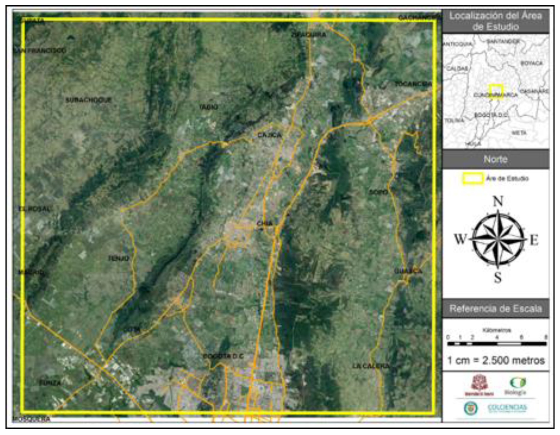
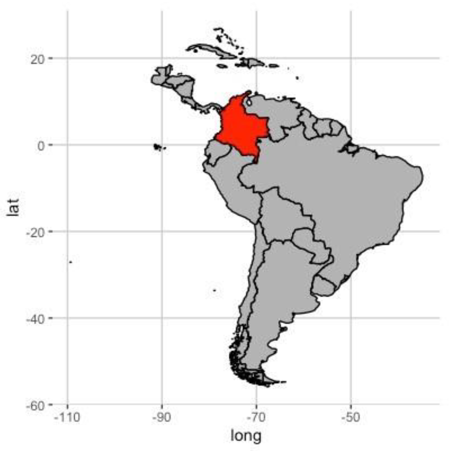
2.1. Study Area

The study area was the northern peri-urban or urban-interface area of Bogotá, Colombia (Figure 1). The country of Colombia is also shown, for reference, in Figure 2. The study area also included the eastern Andes mountains and accounted for several land use cover and ecosystem types, located in both mountainous areas and a high elevation plain within the study area. The elevation ranged from 2600 m to 3500 m above sea level. Precipitation varied from about 600 mm per year to 1200 mm per year and had an annual average temperature of 14 °C [32]. The study area included the urban land use and land cover city of Bogotá as different administrative areas and sociodemographic characteristics, as well as the peri-urban areas that surrounded the city, covering an area of approximately 1075 km2 [42]. The city of Bogotá and its surrounding communities within the study area had approximately 7.5 million inhabitants [43]. The study area was one of the country’s key regions for agricultural and industrial production [44]. The area used for the online survey instrument in Section 2.3 extended from coordinates −74.21 latitude (lat), 5.02 longitude (long) to −73.91 lat, 4.73 long.

2.2. Policy Analysis Approach

Analyses were based on two distinct measurements, or metrics, relating to the preferences of various stakeholders for specific ecosystem services and related benefits and policies living in, working, and visiting the study area. In the survey, respondents were required to select five out of nine potential areas of government investment, and then distribute a fixed amount of money across each program they selected (See Section 2.3.2). By doing so, the survey solicited the respondents’ IPs for local and regional governments directing resources towards certain environmental programs.
The survey also analyzed the WTP of an individual by requiring respondents to answer a hypothetical scenario related to an increase in their water bill to fund additional investments in forest resources conservation (See Section 2.3.2). Because the respondents considered the entire bundle of opportunity costs (since they were considering their own income constraints) this was a measurement of WTP [45,46].
Although we considered several ecosystem services that were relevant to this study area, the provision of water resources was of particular interest [2]. Water was the payment mechanism considered by the WTP question and may have also been the most salient question in the IP section as well. Water resources are also important for Bogotá, Colombia, since water security is key for drinking water, food and energy production, and even for conserving biodiversity and wetland habitat [9]. In fact, water and energy security have also been the focus of several large conservation finance projects around Bogotá (i.e., PES) [47].

2.3. Survey and Data

As part of a larger project on peri-urban forest conservation and socio-ecological trajectories, a survey was conducted online using Qualtrics to assess the respondent’s socioeconomic characteristics, ecosystem service perceptions, and opinions concerning key environmental issues in the study area. Additionally, map literacy was assessed [9,25]. Sociodemographic data collected included age, gender, number of years of living in the study region, residence in the study area (yes/no), type of employment, education level, urban or rural residence, and income.
The survey included an interactive map of the study region overlaid with a high-resolution satellite image (Figure 1). Respondents used the map to identify locations in the study area, including those of environmental amenities [20]. The survey was pretested with 14 experts and then the finalized instrument was sent to an email list during the period of November 2018–February 2019. Reminders to non-respondents to the survey were also sent in mid-December and early January to account for a period of national holidays. The survey was sent out to a total of 4532 e-mails from a list provided by Bogotá’s District Secretariat for Planning. A total of 2359 respondents completed the entire survey, for a response rate of 52%. The Secretariat’s e-mail list contained the addresses of different stakeholders interested in, or who had participated in, governance-related issues in and around Bogotá. Using snowball sampling, the survey instrument was also forwarded by e-mail recipients to other respondents in and around Bogotá. See Section 2.3.2 for the sociodemographic characteristics of these survey instrument respondents.

2.3.1. Spatial Literacy Questions

The survey calculated a spatial literacy index developed by Escobedo et al. (2022) [20]. Respondents identified and located amenities and locations that were clearly visible on the survey’s online map. After a series of follow up questions regarding their perception of their performance, the respondents’ answers were used to calculate an index of spatial literacy. The index itself was calculated from the distances between the respondent’s answers and the actual locations of the benefits, normalized to vary between 0 and 1. The survey found that the mean spatial literacy index was 0.85 [20], with a value of 1 being a perfect score. For specific details on the spatial literacy index and evaluation of the actual positional accuracy of the three landscapes identified by the respondents, see [20].

2.3.2. Questions regarding Investment Preferences

To assess IPs, survey respondents were asked to hypothetically invest a fixed budget across a set of different ecosystem service-related programs listed in Table 1. Monetary values were reported in Colombian pesos (COP). They were presented with a total of 9 different programs and were asked to invest a hypothetical COP $100 million across 5 of these 9 programs. Specifically, they were asked “If you were the mayor of Bogotá and had a hypothetical budget of COP $100 million to invest in forest conservation related options, how would you distribute the COP $100 million across these different programs and ecosystem benefits (Distribute these funds in a maximum of 5 different programs and benefits)”.
Respondents selected their 5 most preferred programs from Table 1. Afterward, respondents were presented with a fixed amount of money and told to divide the money between each of the 5 programs they previously selected. The summary statistics for both the preliminary (Prelim) and final (Final) datasets are shown in Table 2 and Table 3 Overall, the values were similar between the Prelim and the Final dataset. To assess the representativeness of the survey sample relative to the study area, we also included the means for several analyzed sociodemographic variables from our study area (Table 2).

2.3.3. Questions regarding WTP

Respondents were also given background information explaining the ecological and socioeconomic importance of the upper Andean peri-urban forests surrounding Bogotá. They were then presented with a contextualized question regarding payment: “Would you be willing to pay an additional COP $10,000 in your bi-monthly water bill if you could guarantee greater protection for the forests referenced in the survey material? (Yes or no)”. If the respondent answered “Yes”, a similar question would be presented asking if the individual wanted to pay a higher amount. This process would iterate until either a maximum value was reached (COP $50,000), or the respondent selected “No”. Similarly, if a respondent selected “No”, a similar question would be presented asking if the individual would pay a lower amount. This process would also iterate until either COP $0 was reached, or until the respondent selected “Yes”. The responses and iterations for each respondent were stored, which allowed for the calculation of WTP from the responses by taking the final value the respondent selected “Yes” for, or COP $0 if the respondent always selected “No”.

2.4. Empirical Approach

To model IP, a combination of multivariate nonlinear probit models and a multivariate Ordinary Least Squares (OLS) regression were used. Results from the probit model were then incorporated into the OLS regression to control for respondents’ category selection. A multivariate OLS regression was then used to model WTP. For these analyses, we used R version 4.0.2 [48] and R studio version 1.3.1093 [49].

2.4.1. Modeling Investment Preferences

There were two decisions respondents had to make in order to indicate their IP. First, they selected a program to invest in (from Table 1), and second, they reported the magnitude of their investment from the COP $100 million available. Thus, the decision was made in two stages. Spatial information, or any of the sociodemographic variables, might have affected these two distinct decisions in different ways. Therefore, to investigate these effects, IP was modeled, first as an OLS regression (Equation (1)), and next as a two-stage model with a probit model and an OLS regression where outputs of the probit model were used in the OLS regression (Equations (2) and (3)).
The first model (Equation (1)) was a standard multivariate OLS regression. The coefficients that were obtained from estimating Equation (1) were the effects each variable had on both the selection and magnitude decisions.
M 1 , i z = a 1 , z + β 1 , z S i + γ 1 , z X i + ε i
In Equation (1), M 1 , i z is the magnitude an individual ( i ) invests in a category ( z ), S i is the spatial literacy index, and X i is a set of sociodemographic control variables that include gender, years residing in Bogotá, age, high wages, foreign status, student, and whether the respondent is renting. Further, a 1 , z is a constant, β 1 , z is the parameter estimate on spatial literacy, γ 1 , z is a collection of parameter estimates on other control variables, and ε i is the error term.
However, spatial literacy, as well as other covariates, could influence the decision to select a category for investment in a different way than the preferred magnitude of investment. Equation (1) would not be able to disentangle the effects of each variable on both the selection and magnitude decisions separately. Therefore, a two-stage model that specifies and estimates a set of probit models for each category was selected (Table 1). The probit model was able to estimate the probability respondents selected a given category, consistent with a Heckman two-step approach [50]. Equation (2) presents a probit model for a given investment category.
prob ( I i z = 1 ) = a 2 , z + β 2 , z S i + γ 2 , z X i + ε i
In Equation (2), I i z is an indicator that equals 1 if there is any investment in that category, and 0 otherwise. The z index denotes the category of investment (e.g., water quality, forest protection, landscape legacy, etc.).
Following the Heckman two-step procedure [50], probit models were used to generate an Inverse Mills Ratio (IMR) [48]. The IMR was then included as a control variable in Equation (3). The IMR is a measure of the probability of a specific category being selected [41]. Including the IMR in a linear regression provided a way to control for the selection of an IP category z in a multivariate OLS regression [48].
M 2 , i z = a 3 , z + β 3 , z S i + δ z IMR i , z + γ 3 X i + ε i
In Equation (3), the coefficient on the IMR is δ z . Estimating Equation (3) provided the effect of the spatial literacy index on the magnitude of the investment, but conditional on the respondent selecting a given category. This allowed us to assess whether changes in IPs resulting from an individual’s spatial literacy were due to respondents preferring different categories or respondents preferring to invest more money into a category they selected. Estimating Equation (1) provided the average effect (i.e., the effects of the selection and magnitude stages together), whereas Equations (2) and (3) provided a way to separate these effects and report the effects of each variable on both category selection and magnitude of investment.

2.4.2. Modeling Willingness to Pay

An OLS regression was used to examine the drivers of the WTP levels and whether spatial literacy influenced WTP. Because there was no selection stage, a probit model that modeled category selection was not needed.
W i = a 4 + β 4 S i + γ 4 X i + ε i
In Equation (4), W i is WTP, S i is the spatial literacy index, and X i is a set of sociodemographic control variables as reported in Table 2. In Equation (4) a 4 is the constant, β 4 is the parameter estimate on spatial literacy, γ 4 is a collection of parameter estimates on other control variables, and ε i is the error term.

3. Results

The estimation of Equations (1)–(3) (Section 3.1) and Equation (4) (Section 3.2) provided results regarding which variables were statistically significant determinants of IP and WTP. The R2 obtained from estimating Equations (1), (3), and (4) were low. Although these models should not be used to predict the WTP or magnitudes of IP, the aim of our econometric-based analysis was to understand the marginal effects of spatial literacy, as well as the other control variables, on IP and WTP. Thus, as is typical in econometric analyses, the R2 value was a secondary concern relative to the statistical significance and magnitude of the explanatory variables’ coefficients. A preliminary analysis that examined the correlations between IP variables, WTP, and sociodemographic variables can be found in Appendix B.

3.1. Investment Preference Models

Summaries of the results from estimating Equations (1)–(3) are presented in Table 4, Table 5 and Table 6. For each IP category, Table 4, Table 5 and Table 6 report whether the spatial literacy index was significant and the value and level of statistical significance of the coefficient for the spatial literacy index, as well as a list of other statistically significant variables. The regression results were reported in Appendix C.
Overall, spatial literacy had a statistically significant effect (p value < 0.01) on three policy categories: agricultural production, landscape legacy, and water supply programs (Table 4). A higher spatial literacy reduced the IP in agricultural production and wood and timber production; however, it increased the preferred investment in water supply programs. Higher spatial literacy also increased the preferred investment in landscape legacy. There was no consistent effect of sociodemographic variables on preferences for government investment.
The summary for estimating Equation (2) can be found in Table 5. Higher spatial literacy resulted in respondents being less likely to select agricultural production, water supply programs, and environmental education. Conversely, higher spatial literacy resulted in respondents being more likely to select the landscape legacy and recreation and ecotourism categories (Table 5). Estimating Equation (2) found a similar set of inconsistent results in Table 5 as in Table 4, with respect to the effects of sociodemographic variables. Student status had a statistically significant effect on the selection of environmental education, wood and timber production, natural disaster mitigation, and climate change categories.
Table 6 reports if the IMR was statistically significant, in addition to whether spatial literacy was significant, the coefficient on spatial literacy, and the list of other statistically significant control variables. Results indicated that spatial literacy had an effect on magnitudes for three out of the nine investment program categories (agricultural production, environmental education, and wood and timber products). Higher spatial literacy reduced the magnitudes of preferred investment for agricultural production, environmental education, and wood and timber products Sociodemographic variables had a mixed effect on investment preferences for different categories (Table 6). The IMR was statistically significant in agricultural production, environmental education, and wood and timber products.

3.2. Willingness to Pay Model

We found that the effects of several sociodemographic characteristics on WTP were statistically significant (Table 7). For example, the older a respondent was, the lower their WTP for investments in forest resources conservation. This implied that an increase of 1 year in age would decrease WTP by a mere COP $76. However, results found that moving into the high wage category, high education category, or student status would increase WTP. Whether the respondent was a resident of Bogotá, a foreigner, or rented a home (as opposed to owning a home) had no statistically significant effect. Most notably, we did not find a statistically significant effect of the spatial literacy index on WTP.

4. Discussion

This study explored how spatial information regarding the location of peri-urban ecosystems and the supply of ecosystem services—and the ability of different stakeholder to discern these—influenced how people valued and preferred ecosystem services. Specifically, their IPs and WTP for government investment in conservation and environmental programs were studied. We found that the spatial literacy index used to assess spatial information did influence IPs in different ways. For agricultural production and wood and forest products, it did indeed affect both the likelihood that an individual preferred these policies and the magnitude, or how much actual funding they preferred the government to invest. For investment in water supply programs, we found that spatial information affected only the probability that an individual selected a given ecosystem service category or policy. Below, we explained these finding relative to the literature and their relevance to ecological and environmental scientists studying peri-urban ecosystem services.
Overall, we found that the more spatial information an individual had, the higher their IP for water supply programs in our peri-urban study region. This was similar to a past study [34] that found that individuals identified higher values (i.e., preferences) for freshwater provision and water regulation. Another study [37] also found that local knowledge (e.g., spatial information) helped individuals identify provisioning services (e.g., water) and cultural ecosystem services (e.g., recreation). Conversely, another study [41] found that residents were often reluctant to invest in conservation-related activities and programs in public urban green areas in Bogotá, due to the perception of corruption, lack of trust in government, and the ineffectiveness of institutions (i.e., weak governance). However, we were not able to determine whether concerns about weak governance contributed to the lack of statistical significance in our results, as shown in Table 4.
We also found that the effects of spatial information differed between our IP and WTP metrics. Although the two metrics were similar, as explained in our introduction (i.e., they both corresponded to a preference for investment for ecosystem services), there were several clear and important distinctions that needed to be made. First, WTP is a more accepted metric for monetary valuation, since it is based on an individual’s own budget limitations and can reflect the actual price for a certain good or service [51]. In contrast, the IP metric was not based on an individual’s own budget constraint but instead on their preferences for a policy. As such, the IP metric reflects an actual monetary amount that is preferred by an individual, but it is based on the government’s (not the individual’s own) budget limitations and, as such, cannot be considered an actual metric of WTP. This difference between the two metrics likely contributed to differences in the effects. That said, the results of this paper contributed to previous studies regarding valuation and policy preferences.
However, we did not find evidence that spatial literacy influenced our WTP metric for investments in forest conservation (Table 7), despite several sociodemographic characteristics (e.g., age and high wage) having a statistically significant effect on WTP. That is, the older an individual was, the less they were willing to pay for investments in forest conservation. Student status also increased WTP. This might have been due to unobserved political affiliations of the respondents, as past research has shown that political affiliation influences respondents’ WTP [25]. Thus, although information is necessary for valuation processes, our results suggested that the type of information (i.e., spatial, contextual) was also important [52], and that not all information was internalized by individuals in the same way. For example, other types of information, such as education programs or deliberative participatory activities [e.g., 24], might have produced different results. This merits future research. These WTP findings could have implications for citizens’ willingness to use their own funds for PES programs to conserve and manage peri-urban watersheds and to sustain the provisioning and regulating ecosystem services they provide.
Regarding the sources of ecosystem service supply, we found that information about the location of peri-urban ecosystem services in Bogotá influenced respondent’s preferences for government conservation programs, both in terms of which policies and what magnitude of investments were preferred. This was corroborated by another study on policy communication using spatial data as an instrument [53] and also highlighted that such activities could positively influence preferences for these types of policies. This finding has implications for other types of ecosystem services and in contexts other than Bogotá. Furthermore, having spatial information could help develop relevant PES programs that could encourage participation and compliance, which would, in turn, lead to more benefits for landowners and society.
Indeed, there is a growing trend in the use of spatial information for the management of parks and protected areas [54]. For example, Wolf et al., 2015 [53] found that spatial information provided a cost-effective approach for decision making and prioritizing future management strategies. Because the spatial information that a person has access to can be affected by both government/public and private investment [55], the results of this study indicated that this kind of investment could change preferences for government policy [56,57], particularly with respect to environmental issues. Notably, though the effect was statistically significant for IPs (Table 4, Table 5 and Table 6), we did not find that it changed the WTP (Table 7). It might be the case that more information on the sociodemographic characteristics of respondents, or information about the political context in Bogotá might have had a causal relationship with WTP and IP [41]. The inclusion of cartographic and spatial literacy learning objectives in environmental education programs might also be warranted.
We note that our study did have several limitations. First, the metric for WTP, though collected through a standard stated preference survey, might have been biased due to the fact that the starting COP$ value for the WTP question were the same for all respondents. Although this might not be of relevance to ecologists and ecosystem service modelers, this is often a concern in economic valuation studies. Accordingly, we included several sociodemographic controls to account for biases in the WTP question. In addition, we found a reasonable distribution of WTP, and that the mean WTP was not the same as the initial WTP value presented in the valuation exercise. This finding indicated that the initial WTP presented in the valuation exercise did not have an effect on the final WTP selected by respondents. Second, as mentioned previously, the IP metric was not a true measure of WTP. Though the IP questions did not capture WTP, both metrics still offered important insights into respondents’ preferences for government programs and policies. Future research is needed to better link sociodemographic characteristics with the spatial literacy index. Future research could also include the role of additional metrics of for other types of information on driving factors behind people’ valuation processes (i.e., deliberative valuation, education programs, democracy, and governance factors).

5. Conclusions

This study explored the role of spatial information via spatial literacy and how it affected survey respondents’ IP and their WTP for ecosystem service-related polices in peri-urban areas. Including spatial information can be useful while implementing public participatory processes, environmental education and planning, nature conservation, and land management. Otherwise, as conventionally done by biophysical scientists that traditionally focus on measuring the supply of ecosystem services—and not considering the degree of information an individual has regarding the spatial location, magnitude of benefits, ecosystem service types, and available ecosystem service conservation programs—might result in an inefficient valuation or policy recommendation.
This study found that although spatial literacy might not statistically influence the commonly used WTP metric, it did make an econometric difference in both the kinds of policies preferred by respondents, as well as the magnitude of government investments preferred by respondents. This could prove key for the conservation and management of peri-urban ecosystems and was relevant for PES programs that are frequently used to fund conservation projects in peri-urban areas through the world to maintain water quality and supply to nearby cities, among other things. This study found that spatial information and sociodemographic characteristics could also be assessed using spatially explicit online surveys, and that they played a role in policy preferences and valuing ecosystem services in peri-urban areas with complex socio-ecological dynamics.
Ecologists traditionally focus on ecosystem form, function, scales, and the supply of ecosystem services. However, this approach commonly ignores the actual preferences of human beneficiaries. That is, this approach often fails to account for the value that diverse groups of people place on these landscapes and services. This study addressed this often overlooked aspect in order to inform biophysical scientists and decision makers of the importance of integrating concepts of space and additional information, as well as interdisciplinary economics approaches and tools to address these issues in highly complex peri-urban ecosystems. Our findings and approach could therefore be used by environmental and land managers to better understand diverse community member’s spatially explicit investment preferences and PES programs for planning and conservation of natural resources. This study also highlighted the potential effectiveness of education campaigns and how they could influence preferences for government spending on the environment, either from private or public groups. Though our results might imply limited effectiveness for education in terms of private participation in conservation, they did show the potential ability of education to use maps or cartographic information to influence preferences for government involvement, both in terms of the kinds of programs and the magnitude of government investment. It is our hope that our findings increase awareness and knowledge of spatial information and local knowledge of place in complex peri-urban ecosystems across different stakeholder groups, such as farmers, environmentalists, educators, resource managers, and recreationists.

Author Contributions

Conceptualization, M.R.S., F.J.E. and J.J.S.; Methodology, M.R.S., F.J.E. and J.J.S.; Software, M.R.S.; Formal Analysis, M.R.S.; Investigation, M.R.S., F.J.E. and J.J.S.; Data curation: M.R.S. and F.J.E.; Writing—original draft preparation: M.R.S. and F.J.E.; Writing—review and editing, M.R.S., F.J.E. and J.J.S.; Project Administration, F.J.E.; Funding Acquisition, F.J.E. All authors have read and agreed to the published version of the manuscript.

Funding

The original survey instrument and work from which this study is based was funded by the Colombian Administrative Department of Science, Technology and Innovation (COLCIENCIAS; Grant 122274558511).

Institutional Review Board Statement

This research and survey instrument was approved by Universidad del Rosario’s Committee of Ethics per 1993’s Resolution 8430 and 2008’s Resolution 2378.

Informed Consent Statement

Informed consent was obtained from all subjects involved in the study entitled, Simulación de dinámicas socio-ecológicas ante escenarios de cambio climático en bosques secundarios peri-urbanos Altoandinos.

Data Availability Statement

The data presented in this study are available on request from the corresponding author F.J.E. The data are not publicly available due to personal information from survey respondents.

Acknowledgments

We thank Guibor Camargo, Fernando Carriazo, and Alejandro Feged-Rivadeneira from the Universidad del Rosario for their role in assisting in the design and implementation of the online survey instrument. We also thank Marius Bottin for his role in developing the spatial literacy index.

Conflicts of Interest

The authors declare no conflict of interest. The funders had no role in the design of the study; in the collection, analyses, or interpretation of data; in the writing of the manuscript, or in the decision to publish the results.

Appendix A

Table A1. Comments and links to data sources for sociodemographic data reported in Table 2 of the main text.
VariableComments (Source)
FemaleAverage for Bogota DC. (https://www.ccb.org.co/observatorio/Analisis-Social/Analisis-Social/Poblacion-pobreza-y-desigualdad/En-los-rangos-de-edad-mas-jovenes-hay-mayor-numero-de-poblacion-masculina) (accessed on 3 July 2022)
Years resided No comparable census information.
Age (years)Average age in Colombia since census data reports age ranges for Bogota and Cundinamarca. (https://www.semana.com/internacional/articulo/cual-es-la-edad-promedio-de-los-actuales-habitantes-del-mundo/293224/) (accessed on 3 July 2022)
wages ($COP)2019 legal monthly minimum wage in Colombia (https://www.mintrabajo.gov.co/prensa/mintrabajo-es-noticia/2019/-/asset_publisher/5xJ9xhWdt7lp/content/salario-m-c3-adnimo-para-2020-ser-c3-a1-de-877.802) (accessed on 3 July 2022)
foreigner (%)Average for Colombia (https://datosmacro.expansion.com/demografia/migracion/inmigracion/colombia) (accessed on 3 July 2022)
Urban (%)Average for Department of Cundinamarca https://www.datos.gov.co/Mapas-(Nacionales/Poblaci-n-Cundinamarca-2017/ggy4-gvse) (accessed on 3 July 2022)
Rentals (%)Average for Colombia (https://www.metrocuadrado.com/noticias/content/mas-del-30-de-colombianos-viven-en-arriendo-2657/) (accessed on 3 July 2022)

Appendix B. Correlation Table

Table A2 presents the correlations between the IP and WTP variables (listed in the first row) and spatial literacy and sociodemographic variables (listed in the first column) that were calculated. We found that age was negatively correlated with WTP, suggesting that older respondents are related to lower WTP quantities. However, student status had a positive correlation with WTP, suggesting that students might have a higher WTP than non-students. If the respondent indicated that they would be willing to pay the additional fee, there was a negative correlation with the amount they would pay, which suggested the higher the tax, the less likely they would be in favor of the policy. Furthermore, spatial literacy had a positive correlation with WTP and willingness to invest in water resources. Though the correlations were not large in magnitude, it is important to note that the size of the correlation coefficient does not imply either a causal relationship, or lack thereof.
Table A2. Correlation coefficients between explanatory variables (columns) and variables of interest (rows). This includes willingness to pay (WTP; row 1), as well as the quantitative values reported as answers to the questions featured in Table 1.
VariableSpatial LiteracyAgeHigh WagesRentingEducationFemaleStudentResidingForeignWould Pay
WTP0.025−0.1690.133−0.0150.02−0.0120.198−0.0830.008−0.425
Agricultural production−0.090.011−0.048−0.014−0.015−0.011−0.011−0.0150.007−0.016
Water supply programs0.0980.064−0.0005−0.030.0020.008−0.0630.055−0.0130.03
Landscape Legacy0.015−0.0120.009−0.0160.0220.0120.0590.0150.019−0.015
Environmental education0.008−0.039−0.0340.042−0.00040.0440.022−0.0650.035−0.02
Wood and timber production−0.1210.0040.005−0.0320.023−0.001−0.0060.0230.0110.045
Natural disaster mitigation0.0080.0460.001−0.0160.0130.043−0.0470.051−0.010.007
Protecting biodiversity0.032−0.024−0.0020.018−0.0020.001−0.012−0.025−0.003−0.024
Climate change−0.034−0.030.0070.041−0.018−0.0280.034−0.032−0.0250.005
Recreation and ecotourism−0.031−0.0420.062−0.009−0.015−0.0770.061−0.0180.001−0.012

Appendix C. Regression Tables

In Table A3, Table A4 and Table A5, we report the regression results for the Investment Preference (IP) models. First, we present the results of average effects model (Table A3), that contains both the effects of spatial information on the selection and magnitude decisions. Table A4 presents results for the probit model from Equation (2). Table A5 presents results from estimating Equation (3).
Table A3. Regression results for the one-stage model. These are the results that are reported in Table 4 of the main manuscript.
AgricultureForestWaterTourismCulturalEnvironmentalNaturalClimateBiodiversity
HistoryEducationRiskChange
spatial literacy−0.074 ***−0.084 ***0.148 ***−0.0310.0140.0160.003−0.0390.046
index(0.018)(0.014)(0.033)(0.019)(0.02)(0.021)(0.023)(0.027)(0.028)
age0.017−0.0150.0.32−0.0020.036−0.0090.0010.007−0.068 *
(0.023)(0.018)(0.042)(0.025)(0.026)(0.028)(0.03)(0.036)(0.037)
high wage−1.019 **0.165−0.1391.286 **−0.077−0.7960.1650.3370.079
(0.458)(0.357)(0.85)(0.499)(0.52)(0.557)(0.593)(0.718)(0.742)
residency−0.020.0160.0130.0090.025−0.040 **0.026−0.012−0.017
(0.016)(0.012)(0.03)(0.017)(0.018)(0.019)(0.021)(0.025)(0.026)
gender0.3140.013−0.1111.659 ***−0.364−1.196 **−1.119 *0.848−0.044
(male = 1)(0.448)(0.349)(0.83)(0.487)(0.508)(0.544)(0.579)(0.701)(0.725)
high-−0.3140.489−0.335−0.2360.5960.0860.228−0.495−0.018
education(0.489)(0.381)(0.908)(0.533)(0.555)(0.595)(0.633)(0.766)(0.792)
student−0.147−0.267−1.3321.235*2.898 ***−0.156−0.7420.868−2.357 **
(0.684)(0.533)(1.27)(0.745)(0.776)(0.832)(0.885)(1.072)(1.108)
foreign0.5041.003−1.5230.2942.0912.731−0.649−3.571−0.881
(1.711)(1.333)(3.175)(1.863)(1.941)(2.081)(2.213)(2.681)(2.771)
rent−0.763−0.602−0.629−0.105−0.1540.579−0.0951.367 *0.403
(0.509)(0.397)(0.945)(0.554)(0.578)(0.619)(0.659)(0.798)(0.825)
constant12.279 ***10.513 ***9.700 ***7.067 ***4.769 **10.226 ***10.984 ***16.026 ***18.435 ***
(1.814)(1.413)(3.366)(1.975)(2.057)(2.206)(2.346)(2.842)(2.937)
Note: n = 2359. standard errors in parentheses. *** p < 0.01; ** p < 0.05; * p < 0.10.
Table A4. Regression results for the first stage probit model of the two-stage model. These are the results that are reported in Table 5 of the main manuscript.
AgricultureForestWaterTourismCulturalEnvironmentalNaturalClimateBiodiversity
HistoryEducationRiskChange
spatial literacy−0.008 ***−0.018 ***0.011 ***−0.004 **0.00030.00004−0.001−0.0020.004 *
index(0.002)(0.002)(0.002)(0.002)(0.002)(0.002)(0.002)(0.002)(0.002)
age−0.003−0.002−0.003−0.002−0.002−0.002−0.002−0.003−0.009 ***
(0.003)(0.003)(0.003)(0.003)(0.003)(0.003)(0.003)(0.003)(0.003)
high wage−0.159 ***0.022−0.0620.079−0.041−0.111 **−0.049−0.026−0.063
(0.055)(0.059)(0.062)(0.054)(0.054)(0.054)(0.054)(0.055)(0.06)
residency−0.003−0.002−0.002−0.0020.001−0.0020.0010.0004−0.00004
(0.002)(0.002)(0.002)(0.002)(0.002)(0.002)(0.002)(0.002)(0.002)
gender0.0780.0570.0040.182 ***−0.04−0.06−0.0550.0830.013
(male = 1)(0.054)(0.057)(0.061)(0.053)(0.052)(0.053)(0.053)(0.054)(0.059)
high-0.0030.086−0.0450.046−0.011−0.0280.035−0.028−0.058
education(0.059)(0.063)(0.066)(0.058)(0.057)(0.058)(0.058)(0.058)(0.064)
student0.0460.030.0590.167 **0.291 ***0.209 ***0.0460.173 **0.009
(0.082)(0.088)(0.092)(0.081)(0.08)(0.081)(0.081)(0.082)(0.091)
foreign0.3130.2040.0520.2140.1540.214−0.146−0.2390.24
(0.2)(0.209)(0.239)(0.2)(0.204)(0.209)(0.2)(0.2)(0.245)
rent−0.139 **−0.154 **−0.101−0.0380.0040.118 *0.0310.0320.04
(0.061)(0.066)(0.068)(0.06)(0.06)(0.06)(0.06)(0.061)(0.067)
constant0.565 ***0.909 ***0.1880.0870.0470.2620.424 **0.550 **0.773 ***
(0.217)(0.228)(0.236)(0.214)(0.212)(0.214)(0.215)(0.217)(0.235)
Log Likelihood−1514.12−1278.10−1127.94−1575.88−1605.54−1581.62−1568.47−1520.33−1218.09
χ2 (df = 9)48.51 ***81.97 ***31.70 ***52.07 ***35.33 ***42.58 ***5.3227.80 ***37.11 ***
Note: n = 2359. standard errors in parentheses. *** p < 0.01; ** p < 0.05; * p < 0.10.
Table A5. Results for two-stage model. The second stage is an Ordinary Least Squares regression on the magnitude of investment for a respondent. By including the IMR in the regression, we are controlling for the probability that a respondent selects a given category.
AgricultureForestWaterTourismCulturalEnvironmentalNaturalClimateBiodiversity
HistoryEducationRiskChange
spatial literacy−0.790 **0.298−0.176−0.472 **−0.076 *0.0170.105−0.002−0.079
index(0.315)(0.358)(0.361)(0.198)(0.04)(0.021)(0.254)(0.191)(0.153)
age−0.281 **0.0350.115−0.225 **−0.31−0.0660.1830.0610.226
(0.133)(0.05)(0.102)(0.103)(0.191)(0.082)(0.448)(0.281)(0.354)
high wage−15.201 **−0.3141.6599.472 **−8.354 *−4.3825.2420.7921.897
(6.239)(0.574)(2.171)(3.693)(4.564)(4.843)(12.546)(2.442)(2.305)
residency−0.296 **0.0710.084−0.224 **0.268 **−0.094−0.094−0.02−0.015
(0.122)(0.053)(0.084)(0.105)(0.134)(0.075)(0.297)(0.049)(0.026)
gender7.169 **−1.219−0.19820.449 **−8.415 *−3.1324.609−0.624−0.421
(male = 1)(3.04)(1.206)(0.836)(8.413)(4.44)(2.653)(7.582)(7.582)(0.854)
high-−0.079−1.4011.0384.518 **−1.74−0.784−3.3890.0081.757
education(0.499)(1.811)(1.775)(2.191)(1.395)(1.31)(8.95)(2.691)(2.273)
student3.767 **−0.915−2.92618.037 **60.823 *6.392−5.422−2.123−2.187 *
(1.848)(0.808)(2.178)(7.547)(31.739)(8.825)(11.586)(15.377)(1.127)
foreign27.041 **−3.424−3.02221.628 **32.097 *9.10314.8970.875−7.168
(11.767)(4.358)(3.586)(9.716)(16.55)(8.798)(38.441)(22.965)(8.04)
rent−13.171 **2.7952.346−4.083 **0.7924.268−3.3130.803−0.73
(5.467)(3.209)(3.437)(1.862)(0.776)(4.989)(7.97)(2.998)(1.59)
IMR125.851 **−29.102−72.874151.922 **332.688 *55.079−181.486−32.748−68.158
(55.214)(27.274)(80.935)(67.907)(182.23)(73.897)(448.008)(167.998)(81.808)
constant−37.352 *13.425 ***55.583−104.99 **−250.69 *−24.797110.24431.74443.720
(21.850)(3.073)(51.069)(50.125)(139.948)(47.042)(245.039)(80.682)(30.491)
Note: n = 2359. standard errors in parentheses. *** p < 0.01; ** p < 0.05; * p < 0.10.

References

  1. Sylla, M.; Hagemann, N.; Szewrański, S. Mapping trade-offs and synergies among peri-urban ecosystem services to address spatial policy. Environ. Sci. Policy 2020, 112, 79–90. [Google Scholar] [CrossRef]
  2. Clerici, N.; Cote-Navarro, F.; Escobedo, F.J.; Rubiano, K.; Villegas, J.C. Spatio-temporal and cumulative effects of land use-land cover and climate change on two ecosystem services in the Colombian Andes. Sci. Total Environ. 2019, 685, 1181–1192. [Google Scholar] [CrossRef] [PubMed]
  3. Dobbs, C.; Escobedo, F.J.; Clerici, N.; De La Barrera, F.; Eleuterio, A.A.; MacGregor-Fors, I.; Reyes-Paecke, S.; Vásquez, A.; Camaño, J.D.Z.; Hernández, H.J. Urban ecosystem Services in Latin America: Mismatch between global concepts and regional realities? Urban Ecosyst. 2019, 22, 173–187. [Google Scholar] [CrossRef]
  4. Livesley, S.J.; Escobedo, F.J.; Morgenroth, J. The Biodiversity of Urban and Peri-Urban Forests and the Diverse Ecosystem Services They Provide as Socio-Ecological Systems. Forest 2016, 7, 291. [Google Scholar] [CrossRef]
  5. Grima, N.; Singh, S.J.; Smetschka, B.; Ringhofer, L. Payment for Ecosystem Services (PES) in Latin America: Analysing the performance of 40 case studies. Ecosyst. Serv. 2016, 17, 24–32. [Google Scholar] [CrossRef]
  6. Redford, K.H.; Adams, W.M. Payment for Ecosystem Services and the Challenge of Saving Nature. Conserv. Biol. 2009, 23, 785–787. [Google Scholar] [CrossRef]
  7. de Castro-Pardo, M.; Azevedo, J.C.; Fernández, P. Ecosystem Services, Sustainable Rural Development and Protected Areas. Land 2021, 10, 1008. [Google Scholar] [CrossRef]
  8. Anselm, N.; Brokamp, G.; Schütt, B. Assessment of land cover change in peri-urban high andean environments South of Bogotá, Colombia. Land 2018, 7, 75. [Google Scholar] [CrossRef] [Green Version]
  9. Rodriguez, M.; Bodini, A.; Escobedo, F.J.; Clerici, N. Analyzing socio-ecological interactions through qualitative modeling: Forest conservation and implications for sustainability in the peri-urban bogota (Colombia). Ecol. Model. 2021, 439, 109344. [Google Scholar] [CrossRef]
  10. Pérez-Rubio, I.; Flores, D.; Vargas, C.; Jiménez, F.; Etxano, I. To What Extent Are Cattle Ranching Landholders Willing to Restore Ecosystem Services? Constructing a Micro-Scale PES Scheme in Southern Costa Rica. Land 2021, 10, 709. [Google Scholar] [CrossRef]
  11. Kaffashi, S.; Shamsudin, M.N.; Radam, A.; Yacob, M.R.; Rahim, K.A.; Yazid, M. Economic valuation and conservation: Do people vote for better preservation of Shadegan International Wetland? Biol. Conserv. 2012, 150, 150–158. [Google Scholar] [CrossRef]
  12. Nabatchi, T.; Amsler, L.B. Direct Public Engagement in Local Government. Am. Rev. Public Adm. 2016, 44, 63S–88S. [Google Scholar] [CrossRef]
  13. Tolvanen, H.; Rönkä, M.; Vihervaara, P.; Kamppinen, M.; Arzel, C.; Aarras, N.; Thessler, S. Spatial information in ecosystem service assessment: Data applicability in the cascade model context. J. Land Use Sci. 2016, 11, 350–367. [Google Scholar] [CrossRef]
  14. Tammi, I.; Mustajärvi, K.; Rasinmäki, J. Integrating spatial valuation of ecosystem services into regional planning and development. Ecosyst. Serv. 2017, 26, 329–344. [Google Scholar] [CrossRef] [Green Version]
  15. Bagstad, K.J.; Villa, F.; Batker, D.; Harrison-Cox, J.; Voigt, B.; Johnson, G.W. From theoretical to actual ecosystem services: Mapping beneficiaries and spatial flows in ecosystem service assessments. Ecol. Soc. 2014, 19, 64. [Google Scholar] [CrossRef] [Green Version]
  16. Carlsson, F. Design of Stated Preference Surveys: Is There More to Learn from Behavioral Economics? Environ. Resour. Econ. 2010, 46, 167–177. [Google Scholar] [CrossRef]
  17. Schaafsma, M.; Brouwer, R.; Rose, J. Directional heterogeneity in WTP models for environmental valuation. Ecol. Econ. 2012, 79, 21–31. [Google Scholar] [CrossRef]
  18. Villegas-Palacio, C.; Berrouet, L.; López, C.; Ruiz, A.; Upegui, A. Lessons from the integrated valuation of ecosystem services in a developing country: Three case studies on ecological, socio-cultural and economic valuation. Ecosyst. Serv. 2016, 22, 297–308. [Google Scholar] [CrossRef]
  19. Bateman, I.J.; Mawby, J. First impressions count: Interviewer appearance and information effects in stated preference studies. Ecol. Econ. 2004, 49, 47–55. [Google Scholar] [CrossRef]
  20. Escobedo, F.J.; Bottin, M.; Clerici, N.; Camargo, S.G.; Feged-Rivadeneira, A. Evaluating the role of spatial landscape literacy in public participation processes and opinions on environmental issues and ecosystem services. Environ. Manag. 2022, 69, 244–257. [Google Scholar] [CrossRef]
  21. Dertwinkel-Kalt, M. Salience and health campaigns. Forum Health Econ. Policy 2016, 19, 1–22. [Google Scholar] [CrossRef] [PubMed] [Green Version]
  22. Lau, J.D.; Hicks, C.C.; Gurney, G.G.; Cinner, J.E. Disaggregating ecosystem service values and priorities by wealth, age, and education. Ecosyst. Serv. 2018, 29, 91–98. [Google Scholar] [CrossRef] [Green Version]
  23. Reilly, K.; Adamowski, J.; John, K. Participatory mapping of ecosystem services to understand stakeholders’ perceptions of the future of the Mactaquac Dam, Canada. Ecosyst. Serv. 2018, 30, 107–123. [Google Scholar] [CrossRef]
  24. García-Díez, V.; García-Llorente, M.; González, J.A. Participatory Mapping of Cultural Ecosystem Services in Madrid: Insights for Landscape Planning. Land 2020, 9, 244. [Google Scholar] [CrossRef]
  25. Dupont, D.P.; Bateman, I. Political affiliation and willingness to pay: An examination of the nature of benefits and means of provision. Ecol. Econ. 2012, 75, 43–51. [Google Scholar] [CrossRef]
  26. Escobedo, F.J.; Bottin, M.; Cala, D.; Montoya, D.L.S. Spatial literacy influences stakeholder’s recognition and mapping of peri-urban and urban ecosystem services. Urban Ecosyst. 2020, 23, 1039–1049. [Google Scholar] [CrossRef]
  27. Burkhard, B.; Kroll, F.; Nedkov, S.; Müller, F. Mapping ecosystem service supply, demand and budgets. Ecol. Indic. 2012, 21, 17–29. [Google Scholar] [CrossRef]
  28. Palomo, I.; Martín-López, B.; Zorrilla-Miras, P.; Del Amo, D.G.; Montes, C. Deliberative mapping of ecosystem services within and around Doñana National Park (SW Spain) in relation to land use change. Reg. Environ. Chang. 2014, 14, 237–251. [Google Scholar] [CrossRef]
  29. Darvill, R.; Lindo, Z. Quantifying and mapping ecosystem service use across stakeholder groups: Implications for conservation with priorities for cultural values. Ecosyst. Serv. 2015, 13, 153–161. [Google Scholar] [CrossRef]
  30. Damastuti, E.; de Groot, R. Participatory ecosystem service mapping to enhance community-based mangrove rehabilitation and management in Demak, Indonesia. Reg. Environ. Chang. 2019, 19, 65–78. [Google Scholar] [CrossRef] [Green Version]
  31. Fagerholm, N.; Käyhkö, N. Participatory mapping and geographical patterns of the social landscape values of rural communities in coastal Zanzibar, Tanzania. Fennia 2009, 187, 43–60. [Google Scholar]
  32. Brown, G.; Fagerholm, N. Empirical PPGIS/PGIS mapping of ecosystem services: A review and evaluation. Ecosyst. Serv. 2015, 13, 119–133. [Google Scholar] [CrossRef]
  33. Fagerholm, N.; Eilola, S.; Kisanga, D.; Arki, V.; Käyhkö, N. Place-based landscape services and potential of participatory spatial planning in multifunctional rural landscapes in Southern highlands, Tanzania. Landsc. Ecol. 2019, 34, 1769–1787. [Google Scholar] [CrossRef] [Green Version]
  34. Raymond, C.M.; Bryan, B.A.; MacDonald, D.H.; Cast, A.; Strathearn, S.; Grandgirard, A.; Kalivas, T. Mapping community values for natural capital and ecosystem services. Ecol. Econ. 2009, 68, 1301–1315. [Google Scholar] [CrossRef]
  35. Ruiz-Frau, A.; Edwards-Jones, G.; Kaiser, M. Mapping stakeholder values for coastal zone management. Mar. Ecol. Prog. Ser. 2011, 434, 239–249. [Google Scholar] [CrossRef] [Green Version]
  36. Bagstad, K.J.; Reed, J.M.; Semmens, D.J.; Sherrouse, B.C.; Troy, A. Linking biophysical models and public preferences for ecosystem service assessments: A case study for the Southern Rocky Mountains. Reg. Environ. Chang. 2016, 16, 2005–2018. [Google Scholar] [CrossRef]
  37. Brown, G.; Montag, J.M.; Lyon, K. Public Participation GIS: A Method for Identifying Ecosystem Services. Soc. Nat. Resour. 2012, 25, 633–651. [Google Scholar] [CrossRef]
  38. He, S.; Su, Y. Understanding Residents’ Perceptions of the Ecosystem to Improve Park–People Relationships in Wuyishan National Park, China. Land 2022, 11, 532. [Google Scholar] [CrossRef]
  39. Brown, G.; Weber, D.; de Bie, K. Assessing the value of public lands using public participation GIS (PPGIS) and social landscape metrics. Appl. Geogr. 2014, 53, 77–89. [Google Scholar] [CrossRef]
  40. Brown, G.; Kelly, M.; Whitall, D. Which ‘public’? Sampling effects in public participation GIS (PPGIS) and volunteered geographic information (VGI) systems for public lands management. J. Environ. Plan. Manag. 2014, 57, 190–214. [Google Scholar] [CrossRef]
  41. Pineda-Guerrero, A.; Escobedo, F.J.; Carriazo, F. Governance, Nature’s Contributions to People, and Investing in Conservation Influence the Valuation of Urban Green Areas. Land 2021, 10, 14. [Google Scholar] [CrossRef]
  42. Mendoza, J.E.; Etter, A. Multitemporal analysis (1940–1996) of land cover changes in the southwestern Bogotá High-plain. Landsc. Urban Plan. 2002, 59, 147–158. [Google Scholar] [CrossRef]
  43. DANE Departamento Administrativo Nacional de Estadística de Colombia (Colombian National Administrative Department for Statistics). Censo Nacional 2018. Available online: https://sitios.dane.gov.co/cnpv/app/views/informacion/perfiles/11_infografia.pdf (accessed on 3 July 2022).
  44. Rubiano, K.; Clerici, N.; Norden, N.; Etter, A. Secondary Forest and Shrubland Dynamics in a Highly Transformed Landscape in the Northern Andes of Colombia (1985–2015). Forests 2017, 8, 216. [Google Scholar] [CrossRef] [Green Version]
  45. Champ, P.; Boyle, K.J.; Brown, T.C. A Primer on Nonmarket Valuation; Springer: Dordrecht, The Netherlands, 2017. [Google Scholar]
  46. Loomis, J.; Kent, P.; Strange, L.; Fausch, K.; Covich, A. Measuring the total economic value of restoring ecosystem services in an impaired river basin: Results from a contingent valuation survey. Ecol. Econ. 2000, 33, 103–117. [Google Scholar] [CrossRef]
  47. Rodríguez-De-Francisco, J.C.; Duarte-Abadía, B.; Boelens, R. Payment for Ecosystem Services and the Water-Energy-Food Nexus: Securing Resource Flows for the Affluent? Water 2019, 11, 1143. [Google Scholar] [CrossRef] [Green Version]
  48. R Core Team. R: A Language and Environment for Statistical Computing; R Foundation for Statistical Computing: Vienna, Austria, 2019; Available online: https://www.R-project.org/ (accessed on 3 July 2022).
  49. RStudio Team. RStudio: Integrated Development for R; RStudio: Boston, MA, USA, 2020; Available online: http://www.rstudio.com/ (accessed on 3 July 2022).
  50. Puhani, P. The Heckman Correction for Sample Selection and Its Critique. J. Econ. Surv. 2000, 14, 53–68. [Google Scholar] [CrossRef]
  51. Hanemann, W.M. Willingness to pay and willingness to accept: How much can they differ? Am. Econ. Rev. 1991, 81, 635–647. [Google Scholar] [CrossRef]
  52. Hiebert, J.; Allen, K. Valuing Environmental Amenities across Space: A Geographically Weighted Regression of Housing Preferences in Greenville County, SC. Land 2019, 8, 147. [Google Scholar] [CrossRef] [Green Version]
  53. Wolf, I.D.; Wohlfart, T.; Brown, G.; Lasa, A.B. The use of public participation GIS (PPGIS) for park visitor management: A case study of mountain biking. Tour. Manag. 2015, 51, 112–130. [Google Scholar] [CrossRef]
  54. Beeco, J.A.; Brown, G. Integrating space, spatial tools, and spatial analysis into the human dimensions of parks and outdoor recreation. Appl. Geogr. 2013, 38, 76–85. [Google Scholar] [CrossRef]
  55. Ribaudo, M.; Greene, C.; Hansen, L.; Hellerstein, D. Ecosystem services from agriculture: Steps for expanding markets. Ecol. Econ. 2010, 69, 2085–2092. [Google Scholar] [CrossRef]
  56. Althaus, S.L. Information Effects in Collective Preferences. Am. Political Sci. Rev. 1998, 92, 545–558. [Google Scholar] [CrossRef]
  57. Crook, S.; Levine, A.; Lopez-Carr, D. Perceptions and Application of the Ecosystem Services Approach among Pacific Northwest National Forest Managers. Sustainability 2021, 13, 1259. [Google Scholar] [CrossRef]
Figure 1. Map of the study area used in the Spanish language digital survey comprising northern Bogotá Distrito Capital (D.C.) and the surrounding peri-urban areas.
Land 11 01267 g001
Figure 2. Map of South America, parts of Central America, and the Caribbean, with Colombia highlighted in red, for reference.
Land 11 01267 g002
Table 1. The list of programs and policies in the survey questions regarding government investment in ecosystem services.
Natural disaster mitigation:Invest in programs that control flooding and mitigating mass wasting events
Environmental
education:
Invest in environmental education and nature immersion programs
Agricultural production:Invest in the production of agricultural goods
Climate change:Invest in climate change adaptation programs
Water supply programs:Invest in programs and increase water supply
Wood and timber supply:Invest in fuelwood and timber production program
Landscape legacy and
heritage:
Invest in programs that preserve a landscape’s history and patrimony
Protecting biodiversity:Invest in programs and preserve and conserve biodiversity and natural habitats
Recreation and ecotourism:Invest in programs that promote ecotourism and recreation
Table 2. Sociodemographic characteristics for the survey respondents (n = 2359) in both the Prelim and Final data sets. Study area socio-demographics are also presented. Note: since some of the variables were designed based on the study’s research objectives, many do not have an equivalent in a National- or Regional-level census. Additionally, some means were only available at the Bogotá DC, Department of Cundinamarca, or National level, as indicated in Comments. Links to the sources used to report the study area means are found in websites reported in Appendix A.
VariableMean
(Prelim)
Mean
(Final)
Mean
(Study Area)
Comments (Source)
Female0.580.5450.485Average for Bogota DC.Error! Hyperlink reference not valid.
Years resided 22.75223.633N/ANo comparable census information.
Age (years)33.29834.69831Average age in Colombia, since census data reports age ranges for Bogota and Cundinamarca.
Wages ($COP)5.4725.498N/AWages = the number of legal monthly minimum wages. This number times COP$877,802 = mean monthly household income.
Foreigner (%)0.0210.0170.023Average for Colombia
Urban (%)0.8910.8920.71Average for Department of Cundinamarca
Rentals (%)0.310.3060.35Average for Colombia
Table 3. Descriptive statistics for the Prelim and Final datasets used in the valuation analysis for Bogotá, Colombia. SD, standard deviation; OBS, observations; WTP, willingness to pay; SLI; spatial literacy index. The number of observations for the cleaned dataset are 2359 for each variable reported.
VariableMean
(Prelim)
SD
(Prelim)
OBS
(Prelim)
Mean
(Final)
SD
(Final)
WTP ($COP)14,501.1815,151.85254214,863.5015,213.49
SLI0.8510.12723970.8510.128
Incorrect locations1.8090.9042397N/AN/A
Agricultural production5.68110.27533965.44410.821
Water supply programs22.51418.669339622.77820.102
Landscape Legacy9.29911.87733968.91112.25
Environmental education9.81712.15433969.62713.136
Wood and timber production3.198.17333963.1828.454
Natural disaster mitigation10.90913.06339611.16713.946
Protecting biodiversity18.93816.554339618.77117.451
Climate change13.20815.834339613.77216.894
Recreation and ecotourism6.44411.50533966.34911.788
Table 4. Empirical results for the Ordinary Least Squares model of investment preferences, not controlling for whether an individual selects a given category or not. The results reflect the aggregate effect of category selection and magnitude selection.
Investment ProgramIs Spatial Literacy Statistically Significant?Spatial Literacy CoefficientOther Statistically Significant Variables
Agricultural production Yes−0.074 *Constant
Water supply programs Yes−0.084 *Constant
Landscape Legacy Yes0.148 *Constant
Environmental education No−0.031High wages, gender, student, constant
Wood and timber production No0.014Student, constant
Natural disaster mitigation No0.016Gender, constant
Protecting biodiversity No0.003Gender, constant
Climate change No−0.039Rent, constant
Recreation and ecotourism No0.046Age, student, constant
Note: n = 2359. * p < 0.01.
Table 5. Nonlinear probit model of the probability of a respondent selecting a given category for investing in an ecosystem service program.
Investment ProgramIs Spatial Literacy Statistically Significant?Spatial Literacy CoefficientOther Statistically Significant Variables
Agricultural production Yes−0.008 ***High wage, rent, constant
Water supply programs Yes−0.018 ***Rent, constant
Landscape Legacy Yes0.011 ***No other significant variables
Environmental education Yes−0.004 **gender, student
Wood and timber production No0.0003Student
Natural disaster mitigation No0.00004High wage, student, rent
Protecting biodiversity No−0.001Constant
Climate change No−0.002Student, constant
Recreation and ecotourism Yes0.004 *Age, constant
Note: n = 2359. *** p < 0.01; ** p < 0.05; * p < 0.10.
Table 6. Results for two-stage model. The second stage is an Ordinary Least Square regression on the magnitude of investment for a respondent. By including the Inverse Mills Ratio in the regression, we control for the probability that a respondent selects a given category.
Investment ProgramIs Spatial Literacy Statistically Significant?Spatial Literacy CoefficientIs the Inverse Mills Ratio Significant?Other Statistically Significant Variables
Agricultural production Yes−0.790 **YesAge, high wage, resident, gender, student, foreign, rent, constant
Water supply programs No0.298NoConstant
Landscape Legacy No−0.176NoNo other significant variables
Environmental education Yes−0.472 **YesAge, high wage, resident, gender, high education, student, foreign, constant
Wood and timber production Yes−0.076 *YesHigh wage, resident, gender, student, foreign, constant
Natural disasters No0.017NoNo other significant variables
Protecting biodiversity No0.105NoNo other significant variables
Climate change No−0.002NoNo other significant variables
Recreation and ecotourism No−0.079NoStudent
Note: n = 2359. ** 0.01< p < 0.05; * 0.05< p < 0.10.
Table 7. Ordinary Least Square model results for willingness to pay (WTP) for forest resource improvement in Bogotá, Colombia. Standard errors of the coefficient estimates are reported in parentheses.
VariableDependent Variable: WTP
Spatial literacy index29.468 (24.074)
Age−76.123 ** (31.461)
High wage3340.250 *** (629.831)
Residency23.477 (21.873)
Gender (male = 1)−276.111 (615.111)
High education1226.859 * (672.200)
Student4417.949 *** (940.626)
Foreigner834.787 (2,352.096)
Rent−358.337 (699.960)
Constant11,026.690 (2,493.242)
Note: n = 2359 *** p < 0.01; ** p < 0.05; * p < 0.10.
Publisher’s Note: MDPI stays neutral with regard to jurisdictional claims in published maps and institutional affiliations.

