The Evolution and Determinants of Ecosystem Services in Guizhou—A Typical Karst Mountainous Area in Southwest China

Abstract

Due to rapid urbanization and economic development, the natural environment and ecological processes have been significantly affected by human activities. Especially in ecologically fragile karst areas, the ecosystems are more sensitive to external disturbances and have a hard time recovering, thus studies on the ecosystem services in these areas are significant. In view of this, we took Guizhou (a typical karst province) as the research area, evaluated the ecosystem service value (ESV) according to reclassified land uses and revised equivalent factors, and investigated the determinants of ecosystem services based on geographic detection. It was found that the total ESV showed a prominent increase trend, increasing from 152.55 billion CNY in 2000 to 285.50 billion CNY in 2020. The rise of grain prices due to growing social demands was the main factor in driving the increase of ESV. Spatially, the ESVs of central and western Guizhou were lower with cold spots appearing around human gathering areas, while that of southern and southeastern Guizhou were higher with hot spots that formed in continually distributed woodland. Moreover, the ESV per unit area and its change rate in karst regions were always lower than that in non-karst areas. Precipitation and temperature were the dominant nature factors while cultivation and population density were the main anthropogenic effects driving the evolution of ecosystem services. Therefore, positive human activities as well as rational and efficient land-use should be guided to promote the coordinated and high-quality development of ecology and the economy.

1. Introduction

Ecosystem services refer to the direct and indirect natural environmental conditions and effects provided by ecosystem and ecological processes to maintain human existence [1,2,3], including provisioning, regulating, and supporting, as well as cultural services [4]. However, with the intensification of human activities, ecosystem services have been increasingly affected by land-use change, economic development, population growth, urbanization, and industrialization [5]. Research shows that over the past 50 years, about 60% of global ecosystem degradations are caused by population growth and urbanization [6,7]. Although governments from countries have adopted a series of environmental protection policies to restore ecosystem functions [8,9,10], and some achievements have been made, the ecological and environmental problems cannot be ignored. The ecosystem service value (ESV) is the monetized embodiment of the service provided by natural ecosystems and is considered as a favorable indicator to evaluate regional sustainable development. In the face of severe resource constraints and global warming, converting ecological resources and advantages into ecological assets and economic advantages is particularly important. It means that the accurate accounting of ESV has new practical significance.

Land is an indispensable carrier for supporting urban economic, social, and cultural activities. Land use and cover change (LUCC) could be the most direct manifestation of human impact on the environment. Especially since rapid industrialization and urbanization, land use patterns and intensity have dramatically varied. The structure and function of ecosystems, as well as the ecological processes, have been changed by LUCC [11], and consequently, led to changes in the ESV. Polasky et al. [12] pointed out that the increase in cultivated land is the main reason for the decline of ESV in partial areas of the United States. Gashaw et al. [13] found that land use is closely related to the value of individual ecosystem services; for instance, the conversion of forest to arable land leads to a decrease in gas and climate regulation but an increase in food production and biodiversity conservation. Urbanization also has a great impact on ecosystem services [14,15] and could be reflected in land-use change, e.g., the occupation of ecological land such as high-quality cultivated land by urban construction affects the function of food supply [16,17]. Similarly, the degradation and reduction of wetlands caused by urban expansion has led to a significant decrease in biodiversity [18]. Therefore, as a bridge connecting natural ecosystems and human socioeconomic systems, LUCC and its impacts on both sides have been widely considered in ecosystem services studies [19].

There are two main types of methods for ESV valuation based on land-use change [20]. One is the functional value evaluation method, which uses the per unit price of ecological products to calculate the value of each ecosystem function by adopting economic valuation techniques such as shadow projects, market pricing, carbon taxes, etc. [21]. Due to the specific considerations of the different ecological processes, products, and parameters, this method could be more accurate, but is complex and more suitable for small-scale studies [22,23]. The other is the equivalent factor method, which uses the economic value of the cropland products per unit area as one equivalent value, thereby defining the value coefficients of different lands and multiplying that with each land area to obtain the ESV [24]. Given the lesser data requirement and statistical convenience, this method is mainly used in large-scale assessments [25]. With the development of remote sensing technology, satellite images and aerial photographs are widely applied to ESV research [26,27], thus the spatial and temporal distribution pattern of ESV and the relevant influencing factors have been given more attention [28]. Research shows that [29,30,31], under different climate conditions, vegetation coverage, and urbanization levels, ESVs present obvious spatial heterogeneity, which in China is gradually increasing from the northwest to the southeast and is extremely high in the southwest and northeast [29]. Besides, Li et al. [32] investigated the spatiotemporal changes of ESVs in China and identified the cold–hot spot areas. It was found that high-value hot spots were mainly distributed in the west, while low-value cold spots were situated around the coastal areas, indicating that urbanization plays an important role in the distribution of ESV.

The scope and object of ESV studies have also gradually expanded, covering small administrative divisions [33,34] to national [35] and even global views [24]; or focusing on natural geomorphic units, such as watersheds [23], plains [36], and oases [37]; as well as ecosystem scales, including forests [38], wetlands [39], and farmland [40]. In addition, more and more attention has been paid to specific areas—for instance, karst regions. Hu et al. [41] evaluated the ESVs of karst regions in China during 1992–2015 and found obvious spatial variations, which increased in the northwest and northern southwest but decreased in the northeast and eastern southwest. Chen et al. [42] focused on karst regions in southwest China, estimated the ESVs based on land-use data from 1980 to 2018, and found that ESVs increased at early stages and decreased thereafter. In terms of spatial distribution, ESVs in the west were higher, while that in the other regions presented high–low alternating characteristics from west to east, showing significant spatial autocorrelations during the study period. There are also studies of provinces and cities in karst regions, such as Guizhou [43], Guangxi [44] and Chengdu [45]; however, it is not sufficient and deep enough, and is especially lacking in mechanism research through the comprehensive consideration of nature conditions and human factors driving the evolution of ecosystem services. Due to the special hydrologic and geological conditions in karst areas, it is easy to form a complex landform and fragile ecological environment, which could further restrict human activities and jointly determine the distribution of vegetation and land use. This significantly varies in non-karst areas and was less focused on in previous studies. Furthermore, the karst in China is mainly distributed in the southwestern economically-backward areas, where the demands of economic development and ecological protection are both urgent. Balancing the relationship between ecology and economy is very important. Therefore, this study aims to investigate land-use change and its corresponding ESV evolution in karst areas, and to explore the key natural factors and anthropogenic effects. The results could provide scientific data support and decision-making references for the optimization of land use, the improvement of ecosystem stability, and, finally, the coordinated development of ecology and economy.

2. Materials and Methods

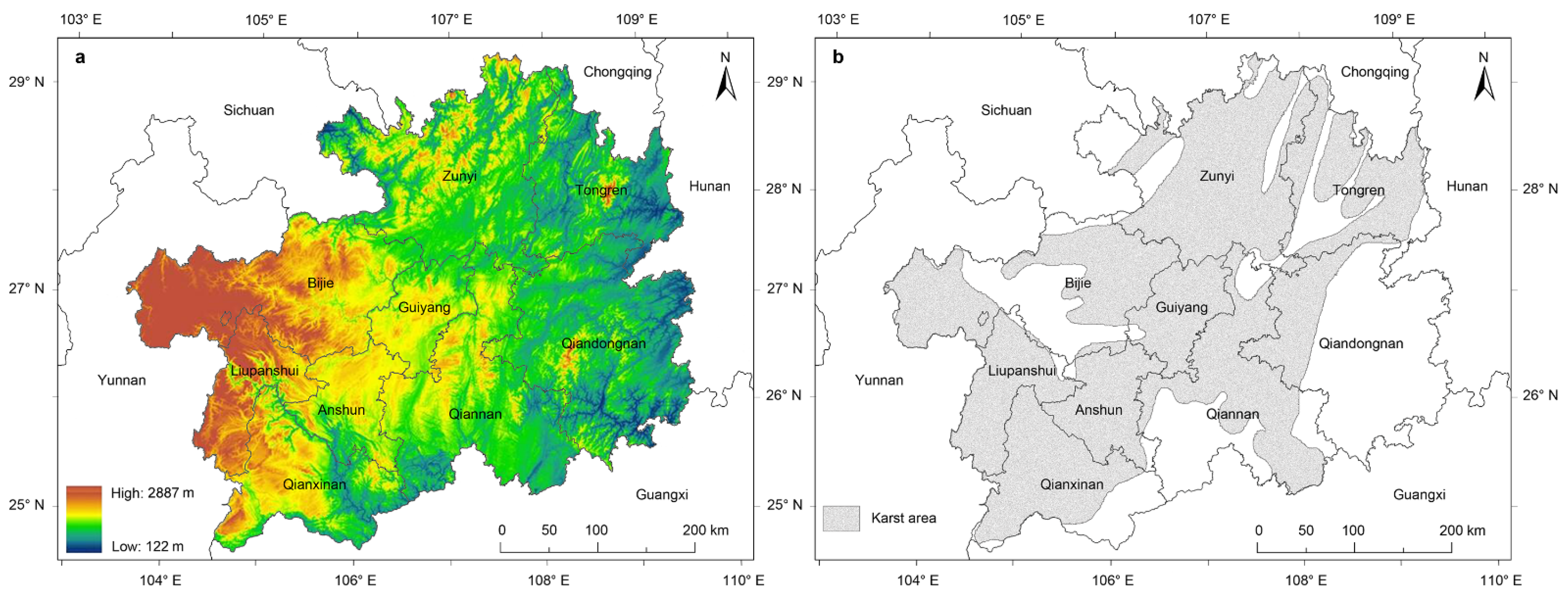
2.1. Study Area

Guizhou province is located in southwest China, with a latitude and longitude of 24°37′–29°13′ N, 103°36′–109°35′ E (Figure 1), and the total area is approximately 176,093 km². It is a mountainous area with high-altitude, low-latitude, and typical karst landforms. The geomorphologic types are dominated by plateau mountains, hills, and basins, with highly undulating terrain, which makes the surface cut in varying degrees. The karst here is widely developed and carbonate outcrops almost 2/3 of the total area (Figure 1b), thus it is an ecologically-fragile area and the vegetation structure has poor stability [46]. The total average elevation is about 1100 m, presenting a general pattern that is higher in the west, lower in the east, and tilts from the middle to the north, east, and south. The topography can be roughly divided into three steps with each average elevation being 1500 m, 800–1500 m, and 800 m, respectively. As in the middle and low-latitude transition zone of the eastern Yunnan–Guizhou Plateau, the climate here is relatively complex. It is influenced by atmospheric circulation and topography, and is divided into a south subtropical climate, a middle subtropical climate, a north subtropical climate, and a warm temperate climate. Most of the study area is located in the middle subtropical and northern subtropical climatic regions, with an annual average temperature of 15 °C, an annual sunshine duration of 1100–1400 h, and an annual average rainfall of 1100–1300 mm. Meanwhile, based on the upper reaches of the Pearl River and the Yangtze River in China, the water resources in Guizhou are relatively rich. However, the engineering water shortage is prominent due to weak water storage capacity from the geological particularity of karst [47].

Guizhou includes one provincial capital city (Guiyang) and eight prefecture cities, with a total permanent population of 37.56 million in 2000 and 38.58 million in 2020. The most populous cities are Bijie (17.89% of the total), Zunyi (17.13%), and Guiyang (15.53%), among which Guiyang has the largest population density. The economics of Guizhou has always been relatively backwards and is lower than the average level of China. Due to the implementation of the “Western Development” strategy in 2000, the socioeconomic development of Guizhou has been significantly improved, which result in the urbanization rate increasing from 23.87% in 2000 to 53.15% in 2020 and the gross domestic product (GDP) increasing from 102.99 billion CNY (2759 CNY per capita) to 1782.66 billion CNY (46,267 CNY per capita), resulting in Guizhou jumping to the forefront of China in terms of its economic growth rate for several years. However, the rapid development of socioeconomic activities also intensified land use and cover changes, thereby increasing the risk of ecosystem functions being damaged and weakened.

In sum, Guizhou is characterized by both ecological vulnerability and a backwards economy, challenging it with the dual tasks of ecological protection and economic development. Therefore, we took Guizhou as the study area, evaluated the ESV according to reclassified land uses and revised equivalent factors, and investigated the determinants of the ecosystem services based on geographic detection. The results could provide an important reference and inspiration for the coordinated and sustainable development of ecology and the economy in similar areas.

2.2. Data Sources and Pre-Processing

In this study, land-use data with a resolution of 1 × 1 km for five periods of 2000, 2005, 2010, 2015, and 2020 were obtained from the Resource and Environment Science and Data Center (RESDC, http://www.resdc.cn, (accessed on 27 July 2021)). According to pre-processing, each land area was extracted and the land, of which was proportional to less than 2%, was merged into the corresponding primary land category to facilitate the statistical analysis; thus, the land-use data were reclassified into nine types, including paddy field, dry land, forest land, shrubbery, sparse wood, grassland, water area, building land, and barren land. Meanwhile, based on previous studies and by combining the regional characteristics of Guizhou with the available data, we preset nine main indicators, including precipitation, temperature, normalized difference vegetation index (NDVI), elevation, slope, lithology, cultivation, population density (PopDensity), and per capita GDP (PerGDP), to comprehensively study the effects of natural factors and human activity on the spatial differentiation of ESV. Among them, elevation and slope were extracted through the DEM data with a resolution of 30 × 30 m, which were obtained from the Geospatial Data Cloud (http://www.gscloud.cn, (accessed on 27 July 2021)). Cultivation was represented by the proportion of farmland per unit area. The rest of the information for the precipitation, temperature, NDVI, lithology, PopDensity, and PerGDP spatialized data, and the administrative boundary vector data, were collected from RESDC. The data above were mainly pre-processed in the ArcGIS 10.7 platform. A fishnet with a grid resolution of 3 × 3 km was created to cut each attribute layer in the study area, and a total of 20,095 grid cells were obtained. The attribute values of every grid corresponding to all layers were measured and extracted to facilitate a subsequent spatial analysis.

In addition, the other relevant socioeconomic development statistics were collected from the Guizhou Provincial Statistical Yearbook, China Agricultural Statistical Yearbook, and China Agricultural Price Survey Yearbook. In order to eliminate the influence of inflation factors on the results, all economic data were revised using the purchasing power index to be comparable to the price in 2000.

2.3. Methods

The framework and procedure adopted in this study are presented in Figure 2. The first step was model selection and data processing. The equivalent factor method was selected based on the available data in Guizhou to assess the ESV, and the equivalent coefficients were revised according to the regional productive and economic factors to get more accurate evaluation results. Thereafter, the land uses were extracted and reclassified based on remote sensing images to suit the selected method, and to highlight the changes in major land uses in Guizhou and their impact on the ESV. The second step was to calculate the ESV, investigate the temporal changes of the ESV, and adopt a sensitivity analysis to verify the applicability of the revised equivalent coefficients. The third step was to match the ESV to the space based on the land-use data and ESV calculation results, reveal its distribution characteristics, and explore the ESV spatial clustering through the spatial autocorrelation analysis. The fourth step was based on the analysis results of the ESV and the selected influencing factors to identify the importance of different natural conditions and human effects. From these steps, the evolution and determinants of ecosystem services in Guizhou could be obtained. The main methods of each step are detailed as below.

2.3.1. Assessment of Ecosystem Service Value

The equivalent factor method originated from Costanza et al.’s [1] evaluation of the global ESV in 1997, which was adapted for research in China. Xie et al. [20] modified the equivalent value coefficients based on the questionnaire survey results of 200 ecologists, and obtained the ecological service value per unit area of terrestrial ecosystems in China, which include forestland, grassland, cropland, wetland, waterbodies, and bare land. Since this method requires few data and adopts relatively uniform standard parameters, the calculation is easy to operate and the results are intuitive and comparable. It is more conducive to analyze the impact of the macro-scale land-use change on ESV evolution. Therefore, the ESV was assessed using the equivalent factor method in this study. Based on the previous studies and combined with the land-use features in Guizhou, nine ecosystems were identified based on land reclassification, merging the land with area that was proportional to less than 2% into a corresponding primary category. Since the ecosystem service of building land is weak, the relevant ESV was considered as 0. The equivalent coefficients of ESV for the rest of the ecosystem and each ecosystem service was decided upon according to previous studies [41,48] and presented in

Table 1. The equivalent coefficients of the ecosystem service value for different land uses.

Ecosystem Service		Farmland		Woodland			Grassland	Water Area	Barren Land
Primary Type	Secondary Type	Paddy Field	Dry Land	Forest Land	Shrubbery	Sparse Wood
Provisioning service	Food	1.36	0.85	0.29	0.19	0.38	0.22	0.80	0.01
	Materials	0.09	0.40	0.66	0.43	0.56	0.33	0.23	0.03
	Water	−2.63	0.02	0.34	0.22	0.31	0.18	8.29	0.02
Regulating service	Air quality regulation	1.11	0.67	2.17	1.41	1.97	1.14	0.77	0.11
	Climate regulation	0.57	0.36	6.50	4.23	5.21	3.02	2.29	0.10
	Waste treatment	0.17	0.10	1.93	1.28	1.72	1.00	5.55	0.31
	Regulation of water flows	2.72	0.27	4.74	3.35	3.82	2.21	102.24	0.21
	Erosion prevention	0.01	1.03	2.65	1.72	2.40	1.39	0.93	0.13
	Maintenance of soil fertility	0.19	0.12	0.20	0.13	0.18	0.11	0.07	0.01
Habitat Service		0.21	0.13	2.41	1.57	2.18	1.27	2.55	0.12
Cultural and amenity service		0.09	0.06	1.06	0.69	0.96	0.56	1.89	0.05
Total		3.89	4.01	22.95	15.22	19.69	11.43	125.61	1.10

.

Specifically, one equivalent coefficient of ESV is defined as 1/7 of the economic value of farmland’s grain per unit area yield, i.e., the monetary embodiment of the equivalent ecological services. According to previous studies [20,41,48], it is generally average data that originates from the national scale over a certain time. For different regions and periods, the variations in productive and economic factors, such as grain types, sown area, yield and prices, etc., could lead to significant differences in the ESV. In order to improve the accuracy of ESV evaluation, scholars modified the equivalent value of ecosystem services in a variety of ways, e.g., comparing grain yield, net profit, normalized difference vegetation index, net primary productivity, precipitation, soil conservation, willingness to pay [49], and so on, making adjustments with global, national, and regional average levels—and in correspondence with expert experience. Therefore, considering the differences in grain products and yields as well as the changes in demand and grain price over time in Guizhou, the equivalent economic value of ecosystem services, i.e., the economic value for one ESV equivalent coefficient, was confirmed through the following formula and presented in

Table 2. The equivalent economic value of ecosystem services revised by the purchasing power index.

Item	2000	2005	2010	2015	2020
Economic value of one equivalent coefficient at current price (CNY/ha)	651.32	1002.48	1282.88	1613.49	1864.55
Purchasing Power Index *	1.00	0.94	0.81	0.71	0.63
Economic value of one equivalent coefficient of comparable price (CNY/ha)	651.32	937.54	1038.31	1137.98	1178.38

* Purchasing Power Index = Reciprocal of the Consumer Price Index (CPI), based on 2000.

:

$$E_a=P_a\frac{1}{7}{{\displaystyle \sum }}_t\frac{m_t{p}_t{q}_t}{M}$$

(1)

where E_a denotes the economic value of ecosystem services corresponding to one equivalent coefficient in year a (CNY/ha); t is the type of grain in the research area (mainly rice, corn, and wheat in Guizhou); m_t, p_t, and q_t represent the sown area (ha), average price (CNY/t), and per unit area yield (t/ha) of each type of grain, respectively; M is the total sown area of grain (ha); and P_a is the purchasing power index in year a based on 2000, which was used to revise the current price to a comparable price.

Combining Table 1 and Table 2, the value coefficient per unit area for each service of different ecosystems in different years as well as the corresponding ESV could be calculated according to the following formulas:

$$ES{V}_{ij}=V{C}_{ij}{A}_i=e_{ij}{E}_a{A}_i$$

(2)

$$ESV={{\displaystyle \sum }}_i{{\displaystyle \sum }}_{j}ES{V}_{ij}$$

(3)

where ESV denotes the ecosystem service value (CNY); i and j refer to the type of ecosystems and ecosystem services, respectively; VC_ij is the value coefficient per unit area for service j in ecosystem i (CNY/ha); A_i is the area of ecosystem i (ha); e_ij is the equivalent coefficient of ESV shown in Table 1; and E_a is the economic value for one ESV equivalent coefficient shown in Table 2 (CNY/ha).

2.3.2. Sensitivity Analysis

It is indispensable to conduct a sensitivity analysis to verify the elasticity between the equivalent value coefficient (VC) of different ecosystems and the total ESV, where the VC was adjusted by increasing or reducing by 50%, respectively, to ascertain the corresponding change in total ESV [50]. The calculation formula is:

$$CS=\left|\frac{\left(ES{V}^{\prime }-ESV\right)/ESV}{\left(V{C}_i^{\prime }-V{C}_i\right)/V{C}_i}\right|$$

(4)

where CS is the sensitivity coefficient; VC and VC’ represent the initial and adjusted value coefficient, respectively; ESV and ESV’ denote the total ecosystem service value before and after the adjustment; and i is the type of ecosystems. If CS < 1, indicating ESV is inelastic for VC, the research results are credible.

2.3.3. Spatial Autocorrelation Analysis

A spatial autocorrelation analysis is generally used to explore the spatial distribution characteristics and heterogeneity of the ESV, including global and local autocorrelations [51]. Specifically, the global autocorrelation is mainly used to measure the spatial correlation and similarity of the attribute values of adjacent grids over an entire region, while the local autocorrelation is used to reflect the local spatial association and identify the hot spots and cold spots [52]. In this study, the Global Moran’s I and Univariate local Moran’s I were applied to characterize the spatial aggregation or discrete distribution of ESV in Guizhou using GeoDa software. Permutation tests (9999) were used for the statistical significance assessment [53]. The calculation is as follows:

$$I=\frac{{{\displaystyle \sum }}_{i=1}^n{{\displaystyle \sum }}_{j=1}^n{\omega }_{ij}\left(x_i-\overline{x}\right)\left(x_j-\overline{x}\right)}{S^2\left({{\displaystyle \sum }}_i{{\displaystyle \sum }}_j{\omega }_{ij}\right)}$$

(5)

$$I_i=\frac{\left(x_i-\overline{x}\right){{\displaystyle \sum }}_{j=1}^n{\omega }_{ij}\left(x_i-\overline{x}\right)}{S^2}$$

(6)

$$S^2=\frac{1}{n}{{\displaystyle \sum }}_{i=1}^n{\left(x_i-\overline{x}\right)}^2$$

(7)

where I and I_i denote the Global Moran’s I and univariate local Moran’s I; n is the number of grid cells; x_i and x_j represent the measured values of grid i and j; $\overline{x}$ is the average value of the grids; ω_ij is the standardized spatial weight matrix between grid i and j; and S² is the variance. The global Moran’s I ranges from −1 to 1. If I is positive, the ESVs tend to cluster together spatially (high values cluster together or low values cluster near to each other), while if I is negative, high values will repel other high values and tend to be near low values; the spatial autocorrelation is more significant when the I absolute value is larger. If I is near zero, the ESV is randomly distributed with no correlation in space.

2.3.4. Geographic Detection

Geographic detection can be used to detect the stratified heterogeneity of the subject being studied or reveal the possible causality between two variables by analyzing the coupling of their spatial distributions [54]. A Geodetector model [55] was applied to explore the correlations between ESV (Y) and the potential driving factors (Xs, nine selected indicators as mentioned above) in this study. Fishnet cutting and stratified sampling were conducted by ArcGIS to extract the corresponding grid values of the ESV and that of the various driving factors. A statistical analysis was then performed through the Geodetector model to identify dominant factors and their interactions with the ESV. Specifically, the factor detector was used to measure the contribution of factors to ESV spatial distribution, while the interaction detector was applied to assess whether the interaction of pairwise factors would weaken or enhance the explanatory power for the ESV spatial distribution. The factor detector model can be expressed as follow:

$$q=1-\frac{1}{N{\sigma }^2}{{\displaystyle \sum }}_{h=1}^L{N}_h{\sigma }_h^2$$

(8)

where q is the explanatory power of factor X on ESV spatial distribution; h is the partition of factor X; L is the number of partitions; N and σ² represent the number of samples and the discrete variance in the entire region; and N_h and σ_h² are the number of samples and the discrete variance in h layer, respectively. The value range of q is [0,1]. If the stratification is generated by factor X, the larger the q is, the stronger the impact of this factor on the ESV spatial distribution. When q is 0, it means there is no spatial relationship between X and Y.

3. Results

3.1. Land-Use Changes in Guizhou Province from 2000 to 2020

For more specific studies, land-use data in Guizhou were extracted and reclassified into nine types, including paddy field, dry land, forest land, shrubbery, sparse wood, grassland, water area, building land, and barren land. Moreover, considering that carbonate rocks are widely distributed in Guizhou and form the typical karst geological and geomorphic features, which may have a significantly different impact on vegetation distribution and land use compared with non-karst regions, we further divided the study area into karst and non-karst regions (Figure 1b) for comparative analysis. The area and proportion of different land uses as well as land-use changes from 2000 to 2020 are presented in

Table 3. The area (km²) of each land use and its proportion (%) in different regions in Guizhou province.

Year	Region	Farmland		Woodland			Grassland	Water Area	Building Land	Barren Land
		Paddy Field	Dry Land	Forest Land	Shrubbery	Sparse Wood
2000	Karst	9619 a(8.30) p	24,923 (21.50)	12,519 (10.80)	29,779 (25.69)	16,629 (14.35)	21,670 (18.70)	287 (0.25)	470 (0.41)	14 (0.01)
	Non-karst	5141 (8.54)	9714 (16.14)	11,246 (18.69)	13,466 (22.38)	9994 (16.61)	10,375 (17.24)	125 (0.21)	92 (0.15)	30 (0.05)
	All region	14,760 (8.38)	34,637 (19.67)	23,765 (13.50)	43,245 (24.56)	26,623 (15.12)	32,045 (18.20)	412 (0.23)	562 (0.32)	44 (0.02)
2005	Karst	9521 (8.21)	25,000 (21.57)	12,620 (10.89)	29,847 (25.75)	17,155 (14.80)	20,973 (18.09)	294 (0.25)	487 (0.42)	13 (0.01)
	Non-karst	5085 (8.45)	9820 (16.32)	11,234 (18.67)	13,560 (22.53)	10,286 (17.09)	9958 (16.55)	124 (0.21)	92 (0.15)	24 (0.04)
	All region	14,606 (8.29)	34,820 (19.77)	23,854 (13.55)	43,407 (24.65)	27,441 (15.58)	30,931 (17.57)	418 (0.24)	579 (0.33)	37 (0.02)
2010	Karst	9482 (8.18)	24,926 (21.50)	12,648 (10.91)	29,784 (25.70)	17,186 (14.83)	21,002 (18.12)	324 (0.28)	545 (0.47)	13 (0.01)
	Non-karst	5082 (8.44)	9785 (16.26)	11,282 (18.75)	13,643 (22.67)	10,290 (17.10)	9819 (16.32)	161 (0.27)	97 (0.16)	24 (0.04)
	All region	14,564 (8.27)	34,711 (19.71)	23,930 (13.59)	43,427 (24.66)	27,476 (15.60)	30,821 (17.50)	485 (0.28)	642 (0.36)	37 (0.02)
2015	Karst	9245 (7.98)	24,725 (21.33)	12,614 (10.88)	29,690 (25.61)	17,126 (14.78)	20,865 (18.00)	342 (0.30)	1291 (1.11)	12 (0.01)
	Non-karst	5016 (8.33)	9720 (16.15)	11,273 (18.73)	13,604 (22.60)	10,272 (17.07)	9780 (16.25)	177 (0.29)	316 (0.53)	25 (0.04)
	All region	14,261 (8.10)	34,445 (19.56)	23,887 (13.56)	43,294 (24.59)	27,398 (15.56)	30,645 (17.40)	519 (0.29)	1607 (0.91)	37 (0.02)
2020	Karst	8294 (7.16)	25,303 (21.83)	14,558 (12.56)	29,940 (25.83)	13,489 (11.64)	21,650 (18.68)	743 (0.64)	1925 (1.66)	8 (0.01)
	Non-karst	4877 (8.10)	9810 (16.30)	12,125 (20.15)	13,408 (22.28)	9507 (15.80)	9534 (15.84)	446 (0.74)	453 (0.75)	23 (0.04)
	All region	13,171 (7.48)	35,113 (19.94)	26,683 (15.15)	43,348 (24.62)	22,996 (13.06)	31,184 (17.71)	1189 (0.68)	2378 (1.35)	31 (0.02)

^a Area of each land use (km²). ^p Area proportion of each land use (%).

and Figure 3. The dominant land uses in Guizhou were woodland, farmland, and grassland, among which woodland (including forest, shrubbery, and sparse wood) was the most widely distributed. Due to the positive ecological policies, woodland always represented more than 1/2 of the total area, followed by farmland (including paddy field and dry land) with a proportion of over 1/4. The water area and building land were very small, while barren land was the smallest—with the proportion only being about 0.02%.

In terms of temporal change, the area of woodland, farmland, grassland, and barren land declined overall during the research period, decreasing by 2.24%, 0.65%, 2.69%, and 29.55%, respectively. Among them, farmland roughly declined period by period, with a maximum decreasing rate of 1.15% from 2010 to 2015. Woodland increased in the early stages and reached a maximum area proportion of 53.85% in 2010; after that, it gradually reduced to a minimum area proportion of 52.83% in 2020, which was opposite to grassland. The total decreasing rate of barren land was the highest, but the change amount was less than 10 km² due to the smallest total area. Contrarily, water area and building land increased significantly, in which, building land presented the highest total change rate—over 300%—increasing from 562 km² in 2000 to 2378 km² in 2020, and growing the fastest from 2010 to 2015 with a rate of 150.31%. Water area exhibited a similar variation trend with building land and had a maximum increasing rate of 129.09% during the last stage. The continuous implementation of the Grain to Green Project in Guizhou is the main reason for the decrease in farmland and the increase in woodland during the early stages, while the rapid urbanization development in the last decade is the key factor that caused the rapid increase in building land. Moreover, the increase in water area is mainly caused by the water storage in reservoirs in the Central Guizhou Water Conservancy Project.

Given the unique karst mountain landform in Guizhou, the land surface is cut to varying degrees and fluctuates greatly, thus forming an obviously fragmented distribution of land use. According to Figure 3, woodland was mainly distributed in the north, east, and south of Guizhou, including some contiguously-distributed forest in the natural reserves, such as the Subtropical Evergreen Broad-leaved Forest National Nature Reserve in the north, Anlong Xianheping National Forest Park in the southwest, and Fanjing Mountain National Nature Reserve in the east. Grassland was more spread out in the western region with higher altitudes, and this type was mostly alpine meadows. Farmland was scattered in gentle slopes and low-lying areas and was closely related to the population distribution. Bijie and Zunyi had the largest population as well as the top three land areas among the nine cities in Guizhou and thus accounted for nearly 40% of the total farmland. Water area was concentrated in the rivers, lakes, and reservoirs of the Wujiang River system and Hongshuihe River system, while building land was intensively distributed in each central city area, especially within the Central Guizhou Cities Group.

Moreover, it is interesting that the land-use distribution had large differences between karst and non-karst regions. For instance, the proportion of paddy fields in farmland was lower in karst regions than in non-karst areas, while that of dry land was reversed. This is because carbonate rock is resistant to physical weathering but easily dissolved and lost through chemical erosion, thereby causing the slowness of the soil-forming process and thus the shallow and discontinuous soil. In general, paddy fields require thicker and relatively concentrated soil relative to dry land, thus representing the distribution features as above. Similarly, in karst regions the proportion of grassland was higher but that of woodland was lower compared to non-karst areas. Meanwhile, the proportion of shrubbery in woodland was significantly higher in karst regions than in non-karst areas. In addition to soil differences, these land-use distribution characteristics are also related to the extensively developed fissures and pipes in karst regions, where rainfall tends to move underground with less surface water storage and weak soil-water holding capacity, which is more suitable for the development of low-water-demand grassland and shrubbery.

3.2. Temporal Variations of Ecosystem Service Value in Guizhou Province from 2000 to 2020

3.2.1. Variations of Ecosystem Service Value in Different Ecosystems

During the research period, the total ESV in Guizhou showed a significant increase from 152.55 billion CNY in 2000 to 285.50 billion CNY in 2020 (

Table 4. The ecosystem service value (billion CNY) of each land use and its proportion (%) in Guizhou province.

Land Use Type	2000		2005		2010		2015		2020
	ESV	%	ESV	%	ESV	%	ESV	%	ESV	%
Paddy field	3.74	2.45	5.33	2.42	5.88	2.40	6.31	2.35	6.04	2.11
Dry land	9.05	5.93	13.09	5.94	14.45	5.90	15.72	5.86	16.59	5.81
Forest land	35.52	23.29	51.33	23.29	57.02	23.27	62.39	23.27	72.16	25.28
Shrubbery	42.87	28.10	61.94	28.10	68.63	28.00	74.99	27.97	77.74	27.23
Sparse wood	34.14	22.38	50.66	22.98	56.17	22.92	61.39	22.90	53.36	18.69
Grassland	23.86	15.64	33.15	15.04	36.58	14.93	39.86	14.87	42.00	14.71
Water area	3.37	2.21	4.92	2.23	6.33	2.58	7.42	2.77	17.60	6.16
Barren land	0.00	0.00	0.00	0.00	0.00	0.00	0.01	0.00	0.00	0.00
Total	152.55	100.00	220.41	100.00	245.07	100.00	268.08	100.00	285.50	100.00

), with an overall growth rate of 87.15%. Among that, the ESV grew the fastest from 2000 to 2005 at an increment of 67.86 billion CNY and a growth rate of 44.48% which was more than half of the overall increase. Thereafter, the ESV growth gradually slowed down and reached a minimum growth rate of 11.42% from 2015 to 2020. Since the economic value of farmland’s grain per unit area yield determines the equivalent economic value of ecosystem services, the rise in grain unit price (comparable price) could be the key factor for the continuous increase of ESV.

Structurally, significant differences in the ESVs among different land uses appeared. As mentioned above, the dominant types of land use in Guizhou were woodland, farmland, and grassland, with their ESV accounting for 93.83–97.79% of the total ESV, and thus playing a decisive role in ecosystem services. In particular, woodland made the greatest contribution, providing 71.20–74.37% of the total ESV (Table 4), while its area only accounted for 52.83–53.85% of the total area (Table 3). Due to the increase in the equivalent economic value of ecosystem services, the ESV of each land use always maintained a rising trend during the study period, except for paddy fields and sparse woods during 2015–2020. However, the detailed contribution of each land use to the total ESV varied differently over time. The area of farmland and grassland gradually decreased, causing its ESV proportion in the total ESV to continuously decrease from 8.38% and 15.64% in 2000 to 7.92% and 14.71% in 2020, respectively. The area of woodland increased during the early stages, leading its ESV proportion in the total ESV to increase from 73.77% in 2000 to 74.37% in 2005, and then gradually decrease to 71.2% in 2020, which was accompanied by the decrease of its area. The above reduced ESV was mainly replaced by the ESV provided from water areas. Though its area was small, water area provided the highest growth rate of ESV, with its proportion climbing from 2.21% up to 6.16% in the total ESV, which was close to the ESV provided by farmland and even exceeded the ESV from paddy fields or dry land, indicating that water area plays more and more of an important role in ecosystem services.

3.2.2. Sensitivity Analysis of the Variations of Ecosystem Service Value

The ranking of the ESV sensitivity index for each land use is woodland, grassland, farmland, water area, and barren land (

Table 5. The sensitivity index resulting from adjustment of equivalent coefficient.

Ecosystem	Sensitivity Index
	2000	2005	2010	2015	2020
Paddy field	0.0245	0.0242	0.0240	0.0235	0.0211
Dry land	0.0593	0.0594	0.0590	0.0586	0.0581
Forest land	0.2329	0.2329	0.2327	0.2327	0.2528
Shrubbery	0.2810	0.2810	0.2800	0.2797	0.2723
Sparse wood	0.2238	0.2298	0.2292	0.2290	0.1869
Grassland	0.1564	0.1504	0.1493	0.1487	0.1471
Water area	0.0221	0.0223	0.0258	0.0277	0.0616
Barren land	0.0000	0.0000	0.0000	0.0000	0.0000

). In the subclass of land use, the highest ESV sensitivity index appears in shrubbery as 0.2810, meaning that the shrubbery in woodland is more sensitive to changes in the ESV equivalent coefficient than other land uses. This is because of the large area of shrubbery in the study area as well as its higher ESV coefficient. Overall, all the ESV sensitivity coefficients are much less than 1.00, indicating that changes in the ESV equivalent coefficients have less impact on the total ESV. Therefore, the ESV equivalent coefficients in this study are basically reliable and applicable, thus the results are credible.

3.2.3. Changes in the Value of Individual Ecosystem Services

From 2000 to 2020, the value of each ecosystem service always presented an upward trend, however, the changes in their proportions in the total ESV showed great differences (

Table 6. The value of individual ecosystem services (billion CNY) and its proportion (%) in Guizhou province.

Ecosystem Service	2000		2005		2010		2015		2020
	ESV	%	ESV	%	ESV	%	ESV	%	ESV	%
Providing Food	5.35	3.51	7.71	3.50	8.53	3.48	9.26	3.46	9.46	3.31
Providing Materials	4.89	3.20	7.06	3.20	7.82	3.19	8.54	3.18	8.83	3.09
Providing Water	−0.20	−0.13	−0.24	−0.11	−0.19	−0.08	−0.10	−0.04	0.86	0.30
Air quality regulation	15.73	10.31	22.70	10.30	25.15	10.26	27.44	10.23	28.16	9.86
Climate regulation	38.73	25.39	55.96	25.39	62.03	25.31	67.76	25.28	69.96	24.50
Waste treatment	12.20	8.00	17.63	8.00	19.57	7.99	21.40	7.98	22.40	7.85
Regulation of water flows	33.98	22.27	49.08	22.27	55.09	22.48	60.52	22.58	70.15	24.57
Erosion prevention	18.37	12.04	26.55	12.04	29.41	12.00	32.12	11.98	33.14	11.61
Maintenance of soil fertility	1.67	1.10	2.41	1.09	2.67	1.09	2.91	1.09	2.99	1.05
Habitat Services	15.15	9.93	21.88	9.93	24.27	9.90	26.51	9.89	27.39	9.59
Cultural and amenity services	6.69	4.39	9.67	4.39	10.72	4.38	11.72	4.37	12.17	4.26

). In terms of the primary type, regulating services were dominant and continuously increased, reaching the highest value of 226.79 billion CNY and the largest proportion of 79.44% in the total ESV in 2020. The value of cultural and amenity services were the lowest, with its maximum proportion being only about 4.39% in the total ESV. The change in provisioning services was consistent with regulating services, where the value and proportion increased simultaneously. However, in habitat services as well as cultural and amenity services, the values gradually increased but their proportions showed an opposite change, reducing by 0.34% and 0.13% in the total ESV during the study period.

For the secondary type of ecosystem service, the ranking of value is as follows: Climate regulation services > Regulation services of water flow > Erosion prevention services > Air quality regulation services > Habitat services > Waste treatment services > Cultural and amenity services > Providing food services > Providing materials services > Maintenance services of soil fertility > Providing water services. Except for the regulation services of water flow exceeding climate regulation services in 2020, the order of individual ecosystem services during the whole period was exactly the same, indicating that the ecosystem structure and function were relatively stable. Climate regulation services had the highest value and were the most dominant ecosystem service, accounting for 47.66% of the total ESV. The lowest value was found in providing water services, which were even negative from 2000 to 2015, manifesting as the utilization and consumption of water resources. The value of providing water services did not turn positive until the substantial increase of water area in 2020, but still only provided 0.30% of the total ESV. Moreover, the value proportions of regulation services of water flow and providing water services gradually increased, which mainly came from the contribution of the increased water area. Inversely, the value proportions of the remaining ecosystem services all decreased from 2000 to 2020, in which the value proportion of the climate regulation services decreased the most, while that of maintenance services of soil fertility decreased the least.

3.3. Spatial Characteristics of Ecosystem Service Values in Guizhou Province from 2000 to 2020

3.3.1. Spatial Distribution and Variations of Ecosystem Service Values

Based on the data and methods above, the ESVs of Guizhou from 2000 to 2020 were further assigned into grids with values of lowest, low, medium, high, and highest to express the spatial distribution characteristics (Figure 4).

The ESVs in Guizhou were generally higher in the east and lower in the west. In 2000, it was dominated by medium and low values, accounting for 45.67% and 30.64% of the total area, respectively, among which low values were mainly distributed in western Guizhou. High values were scattered like plaques in the east and southeast, as well as having a small distribution in the northern and southern edges, which accounted for about 17.79% of the total area. The lowest and highest values were few, while the former was distributed as points near the downtown area and the latter was concentrated in the water area in the central Guizhou reservoirs and the Wujiang River basin. In 2005 and 2010, the medium and low value areas were significantly concentrated in the west; instead, high value areas expanded rapidly on the original basis, and were concentrated and continuously distributed in eastern, southeastern, and southern Guizhou with absolute dominance—and gradually spread to the central and western regions. In 2015 and 2020, the medium and low values were further reduced to 12.09–12.10% and 3.59–4.45% of the total area, and the high values covered 67.33–71.17% of the total area, while the original high value areas in 2000 were gradually transformed into the highest value areas, which accounted for 13.64% of the total area in 2020. The lowest value areas showed little changes during the early stages but increased slightly in 2020 and concentrated near the urban agglomeration of central Guizhou due to urban development and building land expansion. Overall, the spatial differentiation of ESV above is greatly correlated with the topography that is higher in the west and lower in the east, as well as being correlated with the distribution of land use in Guizhou. The temporal evolution of this spatial differentiation is largely affected by the increased equivalent economic value of ecosystem services.

Furthermore, by comparing karst regions with non-karst areas, we found some special and interesting results (

Table 7. The ecosystem service values (billion CNY) and its annual change rate (%) of different regions in Guizhou province.

Region	ESV					Annual Change Rate
	2000	2005	2010	2015	2020	2000–2005	2005–2010	2010–2015	2015–2020	2000–2020
Karst (total)	96.99	140.22	155.70	170.15	180.28	8.92%	2.21%	1.86%	1.19%	4.29%
Karst (CNY/ha) *	8367.40	12,097.49	13,433.09	14,679.14	15,553.61	-	-	-	-	-
Non-karst (total)	55.56	80.19	89.36	97.93	105.21	8.86%	2.29%	1.92%	1.49%	4.47%
Non-karst (CNY/ha) *	9232.49	13,324.27	14,848.69	16,272.06	17,482.15	-	-	-	-	-

* Average ecosystem service value per unit area in karst and non-karst regions.

). In karst regions, the total amount of ESV was higher because of its larger area. However, the average ESV per unit area in karst regions was always lower than in non-karst areas. Similarly, the annual change rate of the ESV was lower in karst areas but higher in non-karst areas, meaning there was a slower growth of the ESV in karst areas. This indicates that geological bases, such as lithology, may have specific effects on the spatial differences and the evolution of ESVs.

3.3.2. Spatial Autocorrelation Analysis of Ecosystem Service Value

According to Geoda software, a global autocorrelation analysis was performed to further explore the spatial distribution and agglomeration of ESVs in the study area. As shown in Figure 5, Moran’s I during the study period was always greater than 0, indicating a positive spatial autocorrelation and agglomeration in ESVs, with high values being adjacent to each other and low values concentrated together. Meanwhile, Moran’s I gradually decreased from 2000 to 2020, meaning that the spatial differences of the ESVs were enhanced and the spatial heterogeneity became larger, especially at the end of the study period, the value points are more scattered, corresponding to the lowest Moran’s I on the scatter plot. Moreover, the value points are mainly distributed in the first and third quadrants, and are more concentrated in the third quadrant, indicating smaller differences between the grids in low value areas. Some of the value points extend along the trend line to the first quadrant, especially in 2020, meaning that the value of some grids increased and were obviously higher than other adjacent grids; this is just matching the rapid evolution of the highest value areas in 2020, as mentioned above.

As can be seen from the cluster map (Figure 6), the difference in the ESV spatial agglomeration in Guizhou was not significant from 2000 to 2015, indicating that the ecosystem structure was relatively stable. ESV hot spots (high–high value areas) were mainly distributed in the east and southeast, and gradually extend along the northwest and southwest directions, showing similarity with the “>” type distribution characteristics. Woodland in these areas was widely distributed, with good ecological integrity and strong ecological service function, which is extremely important for maintaining and improving the regional ecological environment. ESV cold spots (low–low value areas) were mainly distributed in central and northern Guizhou. The land uses in these areas were mainly farmland, accompanied by a large amount of building land with a large population density and strong human disturbance. In addition to protecting basic farmland and ensuring ecological land, the rational development and utilization of urban building land should not be neglected. In 2020, the ESV spatial agglomeration evolved some differences, roughly showing a small contraction of the distribution range of hot spots and cold spots. However, the cold spots in central Guizhou appeared local expansion and connection, which were mainly caused by the rapid agglomeration and development of the cities in central Guizhou, and thus the expanded building land. In future developments, special attention should be paid to the conservation and restoration of ecosystem services in these regions.

3.3.3. Geographical Detection of Spatial Differentiation in Ecosystem Service Values

From the results above, it can be found that ESVs in Guizhou showed obvious spatial differentiation, which is mostly formed under the combination of natural factors such as climate, vegetation, topography, and geology, as well as human activities. On the basis of this, nine potential driving factors were selected for “Factor detection” and “Interaction detection” according to the Geodetector model to further clarify the contribution of these factors to the ecosystem service spatial heterogeneity. The factor detection results (

Table 8. The q statistic and p value of nine factors according to geographical detection.

Factor	2000		2005		2010		2015		2020
	q Statistic	p Value	q Statistic	p Value	q Statistic	p Value	q Statistic	p Value	q Statistic	p Value
Precipitation	0.7820	0.0000	0.7786	0.0000	0.7757	0.0000	0.7687	0.0000	0.7068	0.0000
Temperature	0.6892	0.0000	0.6894	0.0000	0.6831	0.0000	0.6742	0.0000	0.6153	0.0000
NDVI	0.2232	0.0000	0.2426	0.0000	0.2794	0.0000	0.2675	0.0000	0.2472	0.0000
Elevation	0.6363	0.0000	0.6356	0.0000	0.6299	0.0000	0.6243	0.0000	0.5838	0.0000
Slope	0.1617	0.0000	0.1619	0.0000	0.1605	0.0000	0.1584	0.0000	0.1439	0.0000
Lithology	0.1370	0.0000	0.1368	0.0000	0.1355	0.0000	0.1340	0.0000	0.1244	0.0000
Cultivation	0.6552	0.0000	0.6493	0.0000	0.6428	0.0000	0.6346	0.0000	0.5812	0.0000
PopDensity	0.6477	0.0000	0.5032	0.0000	0.6331	0.0000	0.6163	0.0000	0.3611	0.0000
PerGDP	0.1228	0.0000	0.1246	0.0000	0.1293	0.0000	0.0332	0.0000	0.1285	0.0000

) show that each factor has a significant correlation with the spatial distribution of the ESVs, but the respective contribution varies greatly. The multi-year average q value is overall ordered as Precipitation > Temperature > Cultivation > Elevation > PopDensity > NDVI > Slope > Lithology > PerGDP. Among them, Precipitation has the strongest interpretation of the ESV spatial distribution, with each q value exceeding 0.7, followed by Temperature, in which the minimum q value also reaches above 0.6, indicating that climate plays a crucial role in the ESV spatial distribution. In addition, the factors with q values that reach above 0.5 include Elevation, Cultivation, and PopDensity, implying that topography is also a key control factor; furthermore, the influence of human tillage and population density, which reflect the intensity of human activity, cannot be ignored.

Interaction detection is used to investigate whether the combination of any two factors enhance or weaken the strength of the separate interpretation of the ESV spatial distribution. It is shown that each interaction q value is greater than that of a single factor, which further indicates that the spatial distribution of ESVs in Guizhou is the result of the combination of multiple factors. Given the complexity of the data group, we only list the strongest interaction factors in each period (

Table 9. The dominant interaction factors driving the spatial differentiation in ecosystem service values.

Year	Interaction Factors	Interaction q	Interaction Result
2000	Precipitation ∩ Lithology	0.7950	Enhance, bi-
2005	Precipitation ∩ NDVI	0.7937	Enhance, bi-
2010	Precipitation ∩ Lithology	0.7889	Enhance, bi-
2015	Precipitation ∩ Lithology	0.7820	Enhance, bi-
2020	Precipitation ∩ Temperature	0.7202	Enhance, bi-

). The interaction between Precipitation and Lithology, Precipitation and NDVI, and Precipitation and Temperature showed the strongest interpretation of the ESV spatial distribution, with interaction q values all above 0.72, indicating the basic role of natural factors on ESV spatial patterns. The interaction of Precipitation ∩ Lithology is the most prominent, with the highest interaction q value of 0.7950, implying that the difference in lithology would have a great impact on the spatial pattern of ESV under the same precipitation conditions.

4. Discussion

4.1. Mechanism of the Temporal Variation of Ecosystem Service Value

4.1.1. Social Demand

In the assessment of ESV, while the equivalent coefficient is determined, the change of ESV per unit area under the same land use depends on the equivalent economic value of ecosystem services, i.e., determined by the economic value of grain yield per unit area of farmland [29]. In many studies [33,36,42], to focus more on the effect of land-use change on the ESV, the multi-annual average grain price is usually used in the ESV calculation to deduct the impact of price changes on ESV. According to the results of such studies, the ESV variations are generally small, unless there is a large change in land use. Actually, ESV is also the value expression of ecosystem services, which means that the temporal changes and regional differences in grain prices may often bring about huge differences in the ESV [56,57,58]; this cannot be ignored, especially in the ESV evaluation over long timescales. In this study, ESV continuously increased mainly due to the rise of grain unit prices (comparable price). Supposing there is no conversion among different land uses, the increase of ESV caused by the increase of comparable grain unit prices from 2000 to 2020 could be 123.49 billion CNY, about 92.86% of the existing total increment. After deducting the impact of the purchasing power index on prices, this change is largely the value expression of social demand. That is to say, with the development of society and the economy, the disposable personal income and living standards are gradually improved, so thus the quantity and quality of consumer demand enhanced [59]. For ecosystem services, people also potentially have a higher willingness and ability to pay, thus representing a higher ESV.

4.1.2. Land-Use Change

There are significant differences in the ecosystem services under various land uses, corresponding to different ESV equivalent coefficients [20], e.g., the equivalent coefficients of forest land and dry land have a 5-fold gap, while that of water area is even 31-times higher than dry land in this study. In addition, building land is mostly considered a none ecosystem service, thus the ESV is zero [60,61,62]. It follows that, once land use changes, so will ecosystem services and their corresponding value. The staged growth of ESV, where it was faster earlier but slower later in Guizhou, is determined by both the rise of grain prices and the change of land use together. From 2000 to 2010, the continuous afforestation and the Grain to Green Project in Guizhou caused an increase of woodland and thus promoted the growth of total ESV due to the higher ESV equivalent coefficient, which corresponded to a faster growth rate. Obviously, the increase of woodland has a positive effect on ESV. A similar change is particularly significant according to the study of Han et al. [52], in which the land use transfer is dominated by vegetation restoration and has significantly promoted the growth of ESV by nearly 20%. However, during 2010–2020, the development of Guizhou was accelerated and the urbanization rate climbed up rapidly. A large area of land was occupied by the exploitation of building land, offsetting some of the ESV increment caused by rising grain prices, and thus showing a slower growth rate. While in those studies that did not consider the price factors, the transfer of other land to building land usually leads to a direct decline in ESV [34], or maintains a relatively stable ESV through the compensation of ecological land during urban construction [63]. In this study, if the impact of price changes is excluded, the total ESV will increase by 5.25 billion CNY, which is about 3.95% of the current increment. It shows that, despite the recent acceleration of urban construction, the evolution of land use in Guizhou during the research period has an overall positive role on ecosystem services. However, special attention should also be paid to the rational exploitation and efficient utilization of building land to ensure the coordinated and sustainable development of the economy and ecology.

4.2. Driving Factors for the Spatial Differentiation in Ecosystem Service Values

4.2.1. Climate and Vegetation

Climate and vegetation significantly influence ecosystem diversity. Precipitation and temperature are the most intuitive and prominent features of climate, in which the differences in precipitation and temperature among regions constitute an important basis for the spatial differentiation of vegetation and ecosystems. Moreover, as the producer of ecosystems, vegetation determines the complexity of ecosystem structure to a large extent. In general, areas with abundant water and heat conditions are more suitable for developing forest vegetation and forming more complex ecosystems. With the decrease of water and heat, the natural vegetation gradually evolves to grassland and even desert, the ecosystem structure tends to be simple [64], thus the ecosystem services are weakened and the corresponding value is reduced. The precipitation and temperature in Guizhou vary greatly in different regions and are characterized by the monsoon climate. The water and heat are abundant in the east with an average annual rainfall and temperature of 900–1300 mm and 16–18 °C; while that of the western area are lower, about 800–1100 mm and 10–14 °C, respectively. Therefore, the ESV is higher in the east and lower in the west, and the high-value areas are mainly concentrated in the lush forest in eastern and southeastern Guizhou, forming ESV hot spots. This is also well confirmed by the highest q-values of precipitation and temperature according to the geographical detection in this study. The ESV spatial differentiation driven by climate is particularly evident in large-scale studies. According to Xie et al. [29], the ESV in China exhibits a distribution rule corresponding to the zonal vegetation and climate, which gradually decreases from southeastern forest areas with abundant rainfall to northwestern arid vegetation areas and desert, and the difference is significant. Similar to this study, the spatial differentiation of ESV on a meso-scale [36] and small-scale [65] also reflects the effects of topography and regional microclimate, but this spatial difference is much smaller than that of large-scale studies.

4.2.2. Topography and Geology

Topographical and geological conditions have multiple effects on ecosystems. Complex topography is an important factor in causing regional climate differences. The study of Wu et al. [66] on the Qinghai–Tibet Plateau shows that the ESV decreased with an increase in the elevation gradient, and the ESV decreased first and then increased based on the gradient of the slope and terrain niche index, which indicates that the ESV has a significant correlation with the topography. Generally, in the troposphere, air temperature will gradually decrease with the rise of altitude, while the precipitation will increase slightly within a certain elevation range but decrease rapidly thereafter. This is also an important reason for the low average annual temperature and rainfall in the high-altitude area of western Guizhou, which corresponds to the preponderant distribution of alpine meadows and thus the lower ESV. The western mountain land extends along the Miaoling mountains to central Guizhou and slopes to the north, east, and south, leading to gradually increases in water and heat as well as the development of forests—so the ESV is generally higher. On the other hand, the slope and lithology also affect the formation and development of soil as well as the redistribution of surface water and groundwater. Through a study of ESV in northern Guangxi, Zhang et al. [65] found that geology is fundamentally important for ecosystem services and the special geological conditions of karst have different effects on ESV compared to non-karst areas. In karst areas, carbonate rocks are easily dissolved by chemical weathering and transfer with water flow because of its rapid reaction kinetics, leaving less soil parent material, and the soil formation process is slow [67]. Meanwhile, soil particles are also prone to be eroded by water flow on steep mountains, resulting in more debris from primary minerals but less secondary clay minerals in slope soil and the corresponding weak soil water-holding capacity [68]. In addition, widely developed karst fissures will further promote the transfer of surface water underground [69]. However, in the intermountain depression, part of the flushed soil particles accumulate to form a relatively thick soil layer. All the above-mentioned reasons significantly affect the regional distribution of vegetation, thereby explaining the lower ESV per unit area in karst areas than non-karst areas, and the lower ESV on high-slope areas than low-lying areas. To sum up, due to the specific geological and hydrological conditions [70], karst regions are usually characterized by a lack of surface runoff [71], thin soil layer [72], serious soil erosion [73], and weak fertility [74], resulting in low environmental carrying capacity and weak anti-interference ability, as well as poor ecosystem stability [74], with slow vegetation recovery and development, thus showing lower ESV growth than that in non-karst areas.

4.2.3. Human Activities

In addition to the above natural conditions, human activities are also a key factor for local spatial differences in ESV. Guo et al. [75] found that ESV is affected by a combination of the natural environment and human activity, where population is the most important influencing factor of ESV, and the influence of human activities on ESV may be further strengthened through rapid economic development. In our research, the Geodetector results also indicate that there is a high spatial correlation between agricultural activity and population density with ESV. In high altitude mountains and nature reserves, e.g., Fanjing Mountain National Nature Reserve, it is less populated with no cultivation and few disturbances to the ecosystem, natural vegetation such as alpine grassland and native forests are widespread, and the ESV is relatively high. In the foothills with low altitudes and slow slopes, as well as relatively flat areas, which are suitable for farming, the population is concentrated and the vegetation is dominated by farmland as well as sparse wood, shrubbery, and grassland, which are converted from farmland according to the Grain to Green Project, showing relatively low ESV. Especially in Bijie City, which is located in the west of Guizhou and has the largest population as well as the third largest area in the province—most of which are high altitude mountains—the population and farmland are mainly concentrated in the low terrain districts and counties, thus low value areas of ESV are continuously distributed, thereby forming cold spots. In addition, in the central city area of each administrative region, there is a dense population and intense urban construction, and the land use is dominated by building land—except for a small amount of park and greenbelt—thereby presenting the lowest ESV. This is also the main reason for the continuous distribution of ESV cold spots in the Central Guizhou Cities Group. It can be seen that in areas with complex terrain, human activity not only affects ecosystem services but are also restricted by natural conditions. Especially under rapid development, special attention should be paid to avoid irrational development and disorderly human disturbances, which could lead to ecological and environmental destruction and degradation of similar karst mountain areas like Guizhou, and even induce natural and socioeconomic problems such as disaster and poverty [76].

5. Conclusions

During the study period, ESV in Guizhou shows a continuous upward trend, and the increase was faster during the early stages but slowed down during the later stages. Rising social demand reflected by grain prices is the leading factor for ESV increase, contributing to about 92.86% of increment. During the first decade, the continuous implementation of the Grain to Green Project significantly promoted the growth of woodland, which even reached 53.85% of total area, and thus accelerated the rise of ESV. Rapid social and economic development during the latter decade increased the demand for building land, causing over a three-fold rise relative to that in 2000, offsetting some of the growth in ESV. Influenced by natural conditions and human activities, ESV spatial differentiation is significant, with a higher ESV in northern, eastern, and southern regions, and lower ESV in the west. The highest value areas are concentrated in eastern and southeastern Guizhou, which have abundant water and heat conditions and less human activity, thereby forming ESV hot spots. The lowest value areas are continuously distributed in the western mountains with poor water and heat conditions and densely-populated areas in central and western Guizhou, forming cold spots.

Consequently, the spatial and temporal change of ESV is a combination of the results of natural conditions, such as climate, topography, and geology, as well as human activities, such as agricultural activities and urban construction. Natural conditions constitute the basis of ecosystems and ensure the service ceiling they can provide, which is difficult to intervene in. Human activities affect the stability of ecosystem services and determine its lower limit. Positive ecological policies can improve the stability of ecosystem services, and unreasonable development, especially in ecologically sensitive and fragile karst areas, will significantly weaken ecosystem services, which are difficult to recovery. Considering the limitation of land resources and the inevitability of social development, we should persevere in the coordinated development of ecology, society, and the economy: consolidating the achievements of afforestation and protecting ecological land to ensure ecological security, strictly sticking to the farmland red line to ensure food security, and scientifically planning of building land to improve comprehensive land-use efficiency, thereby to achieve high-quality economic development.

This study comprehensively considers the limiting effects of natural conditions and the effects of human activity. Moreover, social demands obviously influenced the value embodiment of ecosystem services and was also taken into account. This could provide methodological references for similar research. In this study, we only investigated the temporal changes of social demands and the relevant impact on ESV; however, the spatial differences of social demands also have significant implications for ecological compensation and economic coordination between regions, which we will take into account in further research.

References

1. Costanza, R.; d’Arge, R.; de Groot, R.; Farber, S.; Grasso, M.; Hannon, B.; Limburg, K.; Naeem, S.; O’Neill, R.V.; Paruelo, J.; et al. The value of the world’s ecosystem services and natural capital. Nature 1997, 387, 253–260. [Google Scholar] [CrossRef]
2. Nelson, E.; Mendoza, G.; Regetz, J.; Polasky, S.; Tallis, H.; Cameron, D.R.; Chan, K.M.A.; Daily, G.C.; Goldstein, J.; Kareiva, P.M.; et al. Modeling Multiple Ecosystem Services, Biodiversity Conservation, Commodity Production, and Tradeoffs at Landscape Scales. Front. Ecol. Environ. 2009, 7, 4–11. [Google Scholar] [CrossRef]
3. Englund, O.; Berndes, G.; Cederberg, C. How to Analyse Ecosystem Services in Landscapes-A Systematic Review. Ecol. Indic. 2017, 73, 492–504. [Google Scholar] [CrossRef]
4. Millennium Ecosystem Assessment. How have ecosystem services and their uses changed? In Ecosystems and Human Well-Being: Synthesis; Island Press: Washington, DC, USA, 2005; pp. 39–48. [Google Scholar]
5. Wang, X.; Yan, F.Q.; Zeng, Y.W.; Chen, M.; Su, F.Z.; Cui, Y.K. Changes in Ecosystems and Ecosystem Services in the Guangdong-Hong Kong-Macao Greater Bay Area since the Reform and Opening Up in China. Remote Sens. 2021, 13, 1611. [Google Scholar] [CrossRef]
6. Harris, J.M. Global environmental challenges of the twenty-first century: Resources, consumption, and sustainable solutions. Ecol. Econ. 2004, 50, 315–316. [Google Scholar] [CrossRef]
7. Wu, J.; Jin, X.; Feng, Z.; Chen, T.; Wang, C.; Feng, D.; Lv, J. Relationship of Ecosystem Services in the Beijing-Tianjin-Hebei Region Based on the Production Possibility Frontier. Land 2021, 10, 881. [Google Scholar] [CrossRef]
8. Deng, L.; Shangguan, Z.P.; Li, R. Effects of the Grain-for-Green program on soil erosion in China. Int. J. Sediment Res. 2012, 27, 120–127. [Google Scholar] [CrossRef]
9. Bai, Y.; Jiang, B.; Wang, M.; Li, H.; Alatalo, J.M.; Huang, S.F. New ecological redline policy (ERP) to secure ecosystem services in China. Land Use Policy 2016, 55, 348–351. [Google Scholar] [CrossRef] [Green Version]
10. Yan, D.; Zhong, C.J. Characteristic of rocky desertification and comprehensive improving model in karst peak-cluster depression in Guohua, Guangxi, China. Procedia Environ. Sci. 2011, 10, 2449–2452. [Google Scholar]
11. Zhao, L.; Liu, J.P.; Tian, X.Z. The temporal and spatial variation of the value of ecosystem services of the Naoli River Basin ecosystem during the last 60 years. Acta Ecol. Sin. 2013, 33, 3169–3176. [Google Scholar] [CrossRef] [Green Version]
12. Polasky, S.; Nelson, E.; Pennington, D.; Kris, A. The Impact of Land-Use Change on Ecosystem Services, Biodiversity and Returns to Landowners: A Case Study in the State of Minnesota. Environ. Resour. Econ. 2011, 48, 219–242. [Google Scholar] [CrossRef]
13. Gashaw, T.; Tulu, T.; Argaw, M.; Abeyou, W.; Tolessa, T.; Kindu, M. Estimating the impacts of land use/land cover changes on Ecosystem Service Values: The case of the Andassa watershed in the Upper Blue Nile basin of Ethiopia. Ecosyst. Serv. 2018, 31, 219–228. [Google Scholar] [CrossRef]
14. Luo, S.F.; Yan, W.D. Evolution and driving force analysis of ecosystem service values in Guangxi Beibu Gulf coastal areas, China. Acta. Ecol. Sin. 2018, 38, 3248–3259. [Google Scholar]
15. Li, L.; Wu, D.F.; Wang, F.; Liu, Y.Y.; Liu, Y.H.; Qian, L.X. Prediction and tradeoff analysis of ecosystem service value in the rapidly urbanizing Foshan City of China: A case study. Acta. Ecol. Sin. 2020, 40, 9023–9036. [Google Scholar]
16. Jiang, L.; Deng, X.; Seto, K.C. The impact of urban expansion on agricultural land use intensity in China. Land Use Policy 2013, 35, 33–39. [Google Scholar] [CrossRef]
17. Huang, Z.H.; Du, X.J.; Castillo, C.S.Z. How does urbanization affect farmland protection? Evidence from China. Resour. Conserv. Recycl. 2019, 145, 139–147. [Google Scholar] [CrossRef] [Green Version]
18. Yan, F.; Zhang, S. Ecosystem service decline in response to wetland loss in the Sanjiang Plain, Northeast China. Ecol. Eng. 2019, 130, 117–121. [Google Scholar] [CrossRef]
19. Zhao, M.; Cheng, W.M.; Huang, K.; Wang, N.; Liu, Q.Y. Research on land cover change in Beijing–Tianjin–Hebei region during the last 10 years based on different geomorphic units. J. Nat. Resour. 2016, 31, 252–264. [Google Scholar]
20. Xie, G.D.; Zeng, L.; Lu, C.X.; Xiao, Y.; Chen, C. Expert Knowledge based Valuation Method of Ecosystem Services in China. J. Nat. Resour. 2008, 23, 911–919. [Google Scholar]
21. Lin, W.P.; Xu, D.; Guo, P.P.; Wang, D.; Li, L.B.; Gao, J. Exploring variations of ecosystem service value in Hangzhou Bay Wetland, Eastern China. Ecosyst. Serv. 2019, 37, 100944. [Google Scholar] [CrossRef]
22. Remme, R.P.; Edens, B.; Schroter, M.; Hein, L. Monetary accounting of ecosystem services: A test case for Limburg province, the Netherlands. Ecol. Econ. 2015, 112, 116–128. [Google Scholar] [CrossRef]
23. Wu, C.; Ma, G.; Yang, W.; Zhou, Y.; Peng, F.; Wang, J.; Yu, F. Assessment of Ecosystem Service Value and Its Differences in the Yellow River Basin and Yangtze River Basin. Sustainability 2021, 13, 3822. [Google Scholar] [CrossRef]
24. Costanza, R.; de Groot, R.; Sutton, P.; van der Ploeg, S.; Anderson, S.J.; Kubiszewski, I.; Farber, S.; Turner, R.K. Changes in the global value of ecosystem services. Glob. Environ. Chang 2014, 26, 152–158. [Google Scholar] [CrossRef]
25. Richardson, L.; Loomis, J.; Kroeger, T.; Casey, F. The role of benefit transfer in ecosystem service valuation. Ecol. Econ. 2015, 115, 51–58. [Google Scholar] [CrossRef]
26. Cabello, J.; Fernandez, N.; Alcaraz-Segura, D.; Oyonarte, C.; Pineiro, G.; Altesor, A.; Delibes, M.; Paruelo, M.G. The ecosystem functioning dimension in conservation: Insights from remote sensing. Biodivers. Conserv. 2012, 21, 3287–3305. [Google Scholar] [CrossRef] [Green Version]
27. Lang, Y.Q.; Song, W. Quantifying and mapping the responses of selected ecosystem services to projected land use changes. Ecol. Indic. 2019, 102, 186–198. [Google Scholar] [CrossRef]
28. Chen, W.; Zeng, J.; Zhong, M.; Pan, S. Coupling Analysis of Ecosystem Services Value and Economic Development in the Yangtze River Economic Belt: A Case Study in Hunan Province, China. Remote Sens. 2021, 13, 1552. [Google Scholar] [CrossRef]
29. Xie, G.D.; Zhang, C.X.; Xiao, Y.; Lu, C.X. The value of ecosystem services in China. Resour. Sci. 2015, 37, 1740–1746. [Google Scholar]
30. Liu, W.; Zhan, J.Y.; Zhao, F.; Yan, H.M.; Zhang, F.; Wei, X.Q. Impacts of urbanization-induced land-use changes on ecosystem services: A case study of the Pearl River Delta Metropolitan Region, China. Ecol. Indic. 2019, 98, 228–238. [Google Scholar] [CrossRef]
31. Chen, F.Y.; Li, L.; Niu, J.Q.; Lin, A.W.; Chen, S.Y.; Hao, L. Evaluating ecosystem services supply and demand dynamics and ecological zoning management in Wuhan, China. Int. J. Environ. Res. Public Health 2019, 16, 2332. [Google Scholar] [CrossRef] [Green Version]
32. Li, G.D.; Fang, C.L.; Wang, S.J. Exploring spatiotemporal changes in ecosystem service values and hotspots in China. Sci. Total Environ. 2016, 545–546, 609–620. [Google Scholar] [CrossRef]
33. Ye, Y.; Zhang, J.; Wang, T.; Bai, H.; Wang, X.; Zhao, W. Changes in Land-Use and Ecosystem Service Value in Guangdong Province, Southern China, from 1990 to 2018. Land 2021, 10, 426. [Google Scholar] [CrossRef]
34. Rahman, M.M.; Szabó, G. Impact of Land Use and Land Cover Changes on Urban Ecosystem Service Value in Dhaka, Bangladesh. Land 2021, 10, 793. [Google Scholar] [CrossRef]
35. Guan, Q.C.; Hao, J.M.; Shi, X.J.; Gao, Y.; Wang, H.L.; Li, M. Study on the change of ecological land and ecosystem service value in China. J. Nat. Resour. 2018, 33, 195–207. [Google Scholar]
36. Zhou, Y.; Zhang, X.; Yu, H.; Liu, Q.; Xu, L. Land Use-Driven Changes in Ecosystem Service Values and Simulation of Future Scenarios: A Case Study of the Qinghai-Tibet Plateau. Sustainability 2021, 13, 4079. [Google Scholar] [CrossRef]
37. Tan, Z.; Guan, Q.Y.; Lin, J.K.; Yang, L.Q.; Lou, H.P.; Ma, Y.R.; Tian, J.; Wang, Q.Z.; Wang, N. The response and simulation of ecosystem services value to land use/land cover in an oasis, Northwest China. Ecol. Indic. 2020, 118, 106711. [Google Scholar] [CrossRef]
38. Taye, F.A.; Folkersen, M.V.; Fleming, C.M.; Buckwell, A.; Mackey, B.; Diwakar, K.C.; Le, D.; Le, D.; Hasan, S.; Ange, C.S. The economic values of global forest ecosystem services: A meta-analysis. Ecol. Econ. 2021, 189, 107145. [Google Scholar] [CrossRef]
39. Ma, X.F.; Zhu, J.T.; Zhang, H.B.; Yan, W.; Zhao, C.Y. Trade-offs and synergies in ecosystem service values of inland lake wetlands in Central Asia under land use/cover change: A case study on Ebinur Lake, China. Glob. Ecol. Conserv. 2020, 24, e01253. [Google Scholar] [CrossRef]
40. Russo, D.; Bosso, L.; Ancillotto, L. Novel perspectives on bat insectivory highlight the value of this ecosystem service in farmland: Research frontiers and management implications. Agric. Ecosyst. Environ. 2018, 266, 31–38. [Google Scholar] [CrossRef]
41. Hu, Z.Y.; Wang, S.J.; Bai, X.Y.; Luo, G.J.; Li, Q.; Wu, L.H.; Yang, Y.J.; Tian, S.Q.; Li, C.J.; Deng, Y.H. Changes in ecosystem service values in karst areas of China. Agr. Ecosyst. Environ. 2020, 301, 107026. [Google Scholar] [CrossRef]
42. Chen, W.; Zhang, X.P.; Huang, Y.S. Spatial and temporal changes in ecosystem service values in karst areas in southwestern China based on land use changes. Environ. Sci. Pollut. R. 2021, 28, 45724–45738. [Google Scholar] [CrossRef] [PubMed]
43. Zhang, T.F.; Wang, L.C.; Su, W.C.; Liang, Y.H.; Shao, J.X.; Zeng, C.F. Analysis of ecological service value in vulnerable karst area of southwestern Guizhou. Adv. Mater. Res. 2012, 1477, 2241–2244. [Google Scholar] [CrossRef]
44. Zhang, M.Y.; Wang, K.L.; Liu, H.Y.; Chen, H.S.; Zhang, C.H.; Yue, Y.M. Responses of ecosystem service values to landscape pattern change in typical Karst area of northwest Guangxi, China. Chin. J. Appl. Ecol. 2010, 21, 1174–1179. [Google Scholar]
45. Dai, X.; Johnson, B.A.; Luo, P.L.; Yang, K.; Yao, Y.Z. Estimation of urban ecosystem services value: A case study of Chengdu, southwestern China. Remote Sens. 2021, 13, 207. [Google Scholar] [CrossRef]
46. Zhang, Y.H.; Xu, X.L.; Li, Z.W.; Liu, M.X.; Xu, C.H.; Zhang, R.F.; Luo, W. Effects of vegetation restoration on soil quality in degraded karst landscapes of southwest China. Sci. Total Environ. 2019, 650, 2657–2665. [Google Scholar] [CrossRef]
47. Peng, T.; Wang, S.J. Effects of land use, land cover and rainfall regimes on the surface runoff and soil loss on karst slopes in southwest China. Catena 2012, 90, 53–62. [Google Scholar] [CrossRef]
48. Xie, G.D.; Zhang, C.X.; Zhen, L.; Zhang, L.M. Dynamic changes in the value of China’s ecosystem services. Ecosyst. Serv. 2017, 26, 146–154. [Google Scholar] [CrossRef]
49. Wang, Y.; Shataer, R.; Xia, T.T.; Chang, X.; Zhen, H.; Li, Z. Evaluation on the Change Characteristics of Ecosystem Service Function in the Northern Xinjiang Based on Land Use Change. Sustainability 2021, 13, 9679. [Google Scholar] [CrossRef]
50. Hu, H.; Liu, W.; Cao, M. Impact of Land Use and Land Cover Changes on Ecosystem Services in Menglun, Xishuangbanna, Southwest China. Environ. Monit. Assess. 2007, 146, 147–156. [Google Scholar] [CrossRef]
51. Hu, X.; Wu, C.; Hong, W.; Qiu, R.; Qi, X. Impact of land-use change on ecosystem service values and their effects under different intervention scenarios in Fuzhou City, China. Geosci. J. 2013, 17, 497–504. [Google Scholar] [CrossRef]
52. Han, X.J.; Yu, J.L.; Shi, L.N.; Zhao, X.C.; Wang, J.J. Spatiotemporal evolution of ecosystem service values in an area dominated by vegetation restoration: Quantification and mechanisms. Ecol. Indic. 2021, 131, 108191. [Google Scholar] [CrossRef]
53. Anselin, L. Local indicators of spatial associationa-LISA. Geogr. Anal. 1995, 27, 93–115. [Google Scholar] [CrossRef]
54. Wang, J.F.; Zhang, T.L.; Fu, B.J. A measure of spatial stratified heterogeneity. Ecol. Indic. 2016, 67, 250–256. [Google Scholar] [CrossRef]
55. Wang, R.S.; Pan, H.Y.; Liu, Y.H.; Tang, Y.P.; Zhang, Z.F.; Ma, H.J. Evolution and driving force of ecosystem service value based on dynamic equivalent in Leshan City. Acta. Ecol. Sin. 2022, 42, 76–90. [Google Scholar]
56. Hu, M.M.; Li, Z.T.; Wang, Y.F.; Jiao, M.Y.; Li, M.; Xia, B.C. Spatio-temporal changes in ecosystem service value in response to land-use/ cover changes in the Pearl River Delta. Resour. Conserv. Recy. 2019, 149, 106–114. [Google Scholar] [CrossRef]
57. Jiang, W.; Wu, T.; Fu, B.J. The value of ecosystem services in China: A systematic review for twenty years. Ecosyst. Serv. 2021, 52, 101365. [Google Scholar] [CrossRef]
58. Liu, H.; Wu, J.; Liao, M. Ecosystem service trade-offs upstream and downstream of a dam: A case study of the Danjiangkou dam, China. Arab. J. Geosic. 2019, 12, 17. [Google Scholar] [CrossRef] [Green Version]
59. Yu, L.; Lyu, Y.; Chen, C.; Choguill, C.L. Environmental deterioration in rapid urbanisation: Evidence from assessment of ecosystem service value in Wujiang, Suzhou. Environ. Dev. Sustain. 2021, 23, 331–349. [Google Scholar] [CrossRef] [Green Version]
60. Qiu, H.H.; Hu, B.Q.; Zhang, Z. Impacts of land use change on ecosystem service value based on SDGs report--Taking Guangxi as an example. Ecol. Indic. 2021, 133, 108366. [Google Scholar] [CrossRef]
61. Hu, Z.N.; Yang, X.; Yang, J.J.; Yuan, J.; Zhang, Z.Y. Linking landscape pattern, ecosystem service value, and human well-being in Xishuangbanna, southwest China: Insights from a coupling coordination model. Golb. Ecol. Conserv. 2021, 27, e01583. [Google Scholar] [CrossRef]
62. Liu, B.; Pan, L.B.; Qi, Y.; Guan, X.; Li, J.S. Land Use and Land Cover Change in the Yellow River Basin from 1980 to 2015 and Its Impact on the Ecosystem Services. Land 2021, 10, 1080. [Google Scholar] [CrossRef]
63. Zhao, D.Y.; Xiao, M.Z.; Huang, C.B.; Liang, Y.; Yang, Z.T. Land Use Scenario Simulation and Ecosystem Service Management for Different Regional Development Models of the Beibu Gulf Area, China. Remote Sens. 2021, 13, 3161. [Google Scholar] [CrossRef]
64. Wen, L.; Song, T.Q.; Du, H.; Wang, K.L.; Peng, W.X.; Zeng, F.P.; Zeng, Z.X.; He, T.G. The succession characteristics and its driving mechanism of plant community in karst region, Southwest China. Acta. Ecol. Sin. 2015, 35, 5822–5833. [Google Scholar]
65. Zhang, M.Y.; Wang, K.L.; Liu, H.Y.; Zhang, C.H.; Yue, Y.M.; Qi, X.K. Effect of ecological engineering projects on ecosystem services in a karst region: A case study of northwest Guangxi, China. J. Clean Prod. 2018, 183, 831–842. [Google Scholar] [CrossRef]
66. Wu, J.H.; Wang, G.Z.; Chen, W.X.; Pan, S.P.; Zeng, J. Terrain gradient variations in the ecosystem services value of the Qinghai-Tibet Plateau, China. Glob. Ecol. Conserv. 2022, 34, e02008. [Google Scholar] [CrossRef]
67. Liu, W.J.; Liu, C.Q.; Zhao, Z.Q.; Li, L.B.; Tu, C.L.; Liu, T.Z. The weathering and soil formation process in karstic area, southwest China: A study on Strontium isotope geochemistry of yellow and limestone soil profiles. J. Earth Environ. 2011, 2, 331–336. [Google Scholar]
68. Yuan, D.X. Aspects on the new round land and resources survey in karst rock desertification areas of South China. Garsologica Sin. 2000, 19, 103–108. [Google Scholar]
69. Zhang, W.; Chen, H.S.; Wang, K.L.; Zhang, J.G. Spatial variability of surface soil water in typical depressions between hills in karst region in dry season. Acta. Pedol. Sin. 2006, 43, 554–562. [Google Scholar]
70. Jiang, Z.C.; Lian, Y.Q.; Qin, X.Q. Rocky desertification in Southwest China: Impacts, causes, and restoration. Earth Sci. Rev. 2014, 132, 1–12. [Google Scholar] [CrossRef]
71. Wu, L.H.; Wang, S.J.; Bai, X.Y.; Tian, Y.C.; Zeng, C.; Luo, G.J.; He, S.Y. Quantitative assessment of the impacts of climate change and human activities on runoff changes in a typical Karst watershed, SW China. Sci. Total Environ. 2017, 601–602, 1449–1465. [Google Scholar] [CrossRef]
72. Ouyang, Z.W.; Song, T.Q.; Peng, W.X.; Du, H.; Zeng, F.P. Spatial heterogeneity of soil main mineral composition in manmade forest in karst peak-cluster depression region. J. Hunan Agric. Univ. 2011, 37, 325–328. [Google Scholar] [CrossRef]
73. Zeng, C.; Wang, S.; Bai, X.; Li, Y.; Tian, Y.; Li, Y.; Wu, L.; Luo, G. Soil erosion evolution and spatial correlation analysis in a typical karst geomorphology, using RUSLE with GIS. Solid Earth 2017, 8, 721–736. [Google Scholar] [CrossRef] [Green Version]
74. Xiong, K.N.; Chi, Y.K. The problems of South China Karst ecosystem in southern China and the countermeasures. Ecol. Econ. 2015, 31, 23–30. [Google Scholar]
75. Guo, C.; Gao, J.; Zhou, B.; Yang, J. Factors of the Ecosystem Service Value in Water Conservation Areas Considering the Natural Environment and Human Activities: A Case Study of Funiu Mountain, China. Int. J. Environ. Res. Public Health 2021, 18, 11074. [Google Scholar] [CrossRef] [PubMed]
76. Wang, R.; Cai, Y.L. Management modes of degraded ecosystem in southwest Karst area of China. Chin. J. Appl. Ecol. 2010, 21, 1070–1080. [Google Scholar]
Figure 1. Location and districts of Guizhou province with topographic condition (a) and karst distribution (b).
Land 11 01164 g001
Figure 2. Framework and procedure adopted in this study.
Land 11 01164 g002
Figure 3. The land-use changes in Guizhou province from 2000 to 2020.
Land 11 01164 g003
Figure 4. The spatiotemporal differentiation of ecosystem service values in Guizhou province from 2000 to 2020.
Land 11 01164 g004
Figure 5. The changes in Global Moran’s I of ecosystem service values in Guizhou province from 2000 to 2020.
Land 11 01164 g005
Figure 6. The local indicators of spatial association cluster maps of ecosystem service values in Guizhou province from 2000 to 2020.
Land 11 01164 g006