Article

Erosion Map Reliability Using a Geographic Information System (GIS) and Erosion Potential Method (EPM): A Comparison of Mapping Methods, BELGRADE Peri-Urban Area, Serbia

by
Nataša Veličković
1,*,
Mirjana Todosijević
1 and
Desanaka Šulić
2
1
Faculty of Forestry, University in Belgrade, 11000 Belgrade, Serbia
2
Faculty of Ecology and Environmental Protection, University Union Nikola Tesla, 11158 Belgrade, Serbia
*
Author to whom correspondence should be addressed.
Land 2022, 11(7), 1096; https://doi.org/10.3390/land11071096
Submission received: 29 May 2022 / Revised: 5 July 2022 / Accepted: 13 July 2022 / Published: 18 July 2022

Abstract

:
Soil erosion is a product of natural and anthropogenic factors and, at the same time, an economic and environmental concern. One of the methods applied to calculate the intensity of erosion is the erosion potential method (EPM), with two possible procedures for determining the average erosion coefficient of an area: analytical and graphical. Using GIS and EPM methods, without field observations of erosion, based on cartographic materials and satellite images, erosion maps were created for 1970 and 2018, for part of the peri-urban area of Belgrade. Based on the created erosion maps, the values of the mean coefficients of erosion, as well as the arithmetic means for the study area, were determined for the settlements. The aim of the study is to assess the reliability of the mean coefficient of soil erosion, obtained from the erosion map created from the cartographic materials and satellite images, without field observations of erosion. Thus, the obtained values of the mean erosion coefficient were compared with the values obtained from the erosion map with field observation and the values obtained by the analytical procedure. Statistical analysis (F test) for 1970 and for 2018 determined a high degree of reliability (p < 0.05) of the mean erosion coefficients of the area obtained from erosion maps that were created from cartographic materials and satellite images without field observation. Regardless of the procedure for determining the mean erosion coefficient, a significant decrease in soil losses was observed, from 10.64 to 5.97 t ha−1year−1 (average annual specific production of sediments, year 1970 and 2018, respectively).

1. Introduction

Soil erosion is the oldest permanent phenomenon of the collapse of the upper layer of the rock mass of the planet Earth, caused by natural and anthropogenic forces. That is a major problem around the world because of its effects on soil productivity, nutrient loss, siltation in water bodies, and degradation of water quality [1]. Furthermore, if erosion is aided by sudden earthquake movements, the period of landscape change is significantly shortened [2]. On the other hand, the deposition of sediments on the river affects reservoirs and dams, increases their costs of maintenance, and, in the long run, makes them unusable [3]. By increasing urban surfaces, permeable surfaces are decreased while excessive forest exploitation and inappropriate soil cultivation disturb the natural soil structure, making favourable conditions for the intensification of soil erosion, rapid surface runoff on slopes, and maximal discharges in river beds [4]. Understanding how these processes occur and what areas are vulnerable to erosion is paramount to land management. Soil erosion models aid land management by helping us understand sediment transport and its effects on a landscape [1]. The planning and implementation of anti-erosion measures and adequate land use are achieved by creating visual models of erosion.
A large number of developed models indicate the importance of solving the problem of soil erosion. Some of the applied models are USLE (Universal Soil Loss Equation) [5], RUSLE (Revised Universal Soil Loss Equation) [6], PESERA (Pan European Soil Erosion Risk Assessment) [7], G2 (Geoland 2) [8], EUROSEM (The European Soil Erosion Model) [9], EPM (Erosion Potential Method) [10,11,12], and others [13,14]. Soil erosion is a very complex process with different interrelated factors and many empirical equations cannot be applied in the same way in different countries despite the efforts of the scientific community to harmonize existing methods and derive a universal method from them [15]. The most widely used approaches during a 40-year history of erosion modelling are the USLE/RUSLE models, which have been applied in 109 countries [16]. The EPM is used by Balkan countries [17,18,19,20,21,22] to assess erosion intensity, and more scientific papers discuss the benefits of applying this method in EU countries [23,24,25,26,27,28], Asia [29,30], Africa [31], and South America [32].
Demonstrating acceptable precision, the EPM makes it possible to identify the areas most sensitive to erosion and degradation processes by including the analysis of the effects of natural factors and anthropogenic activities [20]. The EPM has shown a high degree of reliability and is used as a standard method for mapping erosion for water management purposes (calculating the filling rates of rivers and reservoirs) in the Republic of Serbia. In addition, the method that was researched had to establish a link between erosion-watercourse-sediments, i.e., the link between the intensity of erosion and sediment transport that endangered the rivers and reservoirs. These factors were included in research of the development of the EPM. A summary of the application of the EPM and the quality of the results obtained compared to other methods are presented in [12].
Research on erosion in the Republic of Serbia began in 1954 and was determined by the specifics of the then Socialist Federal Republic of Yugoslavia, with an area of 255,804 km2. On two-thirds of the territory, the slopes were greater than 15% [11], the average annual temperature ranged from +3 °C to +28 °C, and the sum of the annual precipitation was in the range of 260 mm to 5000 mm [33]. For Serbia, slopes exceeded 15% on two-thirds of its territory, the average annual temperature ranged from +3.7 °C to +12.7 °C, the annual precipitation ranged from 557 to 1018 mm, and the amount but not the intensity of precipitation was monitored by weather stations [34].
On the Republic of Serbia’s territory, erosion mapping, for the entire area, was performed for the first time in the period 1966–1971, using a 1:100,000 scale (Table 1, map No. 1). On a cartographic basis (relief and hydrography), the boundaries of erosion areas were mapped by approximate observations in the field, where each erosion area was determined by the degree of erosion endangerment through erosion coefficients. In 1970, the Institute for Cartography “Geokarta”, Belgrade, printed a “Map of soil endangerment by erosion and water”, using a scale of 1:20,000 (Table 1, map No. 2). In 1987, the Institute of Forestry and Wood Industry, Belgrade, Department of Erosion and Land Reclamation, performed an observational mapping of the erosion areas in the vicinity of Belgrade: the basin of the Topčiderska and Bolečka rivers. The erosion areas were plotted into a 1:20,000-scale map from 1967 data according to erosion coefficients. In 2005, the Jaroslav Černi Water Institute, Belgrade, made a 1:100,000-scale erosion map based on aerial images and performed a calculation of the average erosion coefficient via the cadastral municipalities of Belgrade [35]. Authors S. Dragićević and M. Stepić made a 1:50 000 scale erosion map of the Ljig river basin, using a graphical procedure method, based on field observations. In order to have the more objective value of the mean erosion coefficient and apply the Surfer 8 program, they divided the observed site into a grid. [36].
Research on the process of erosion mapping, in order to determine the average erosion coefficient of an area or basin, opens the following questions:
  • Choice of procedure: When should the analytical procedure and when should the graphical one be performed, to determine the average erosion coefficient of an area or basin?
  • Accuracy of erosion coefficient data: Is it to possible to determine erosion coefficients and create an erosion map from cartographic materials, satellite images, or aerial photographs using a GIS, without surveying?
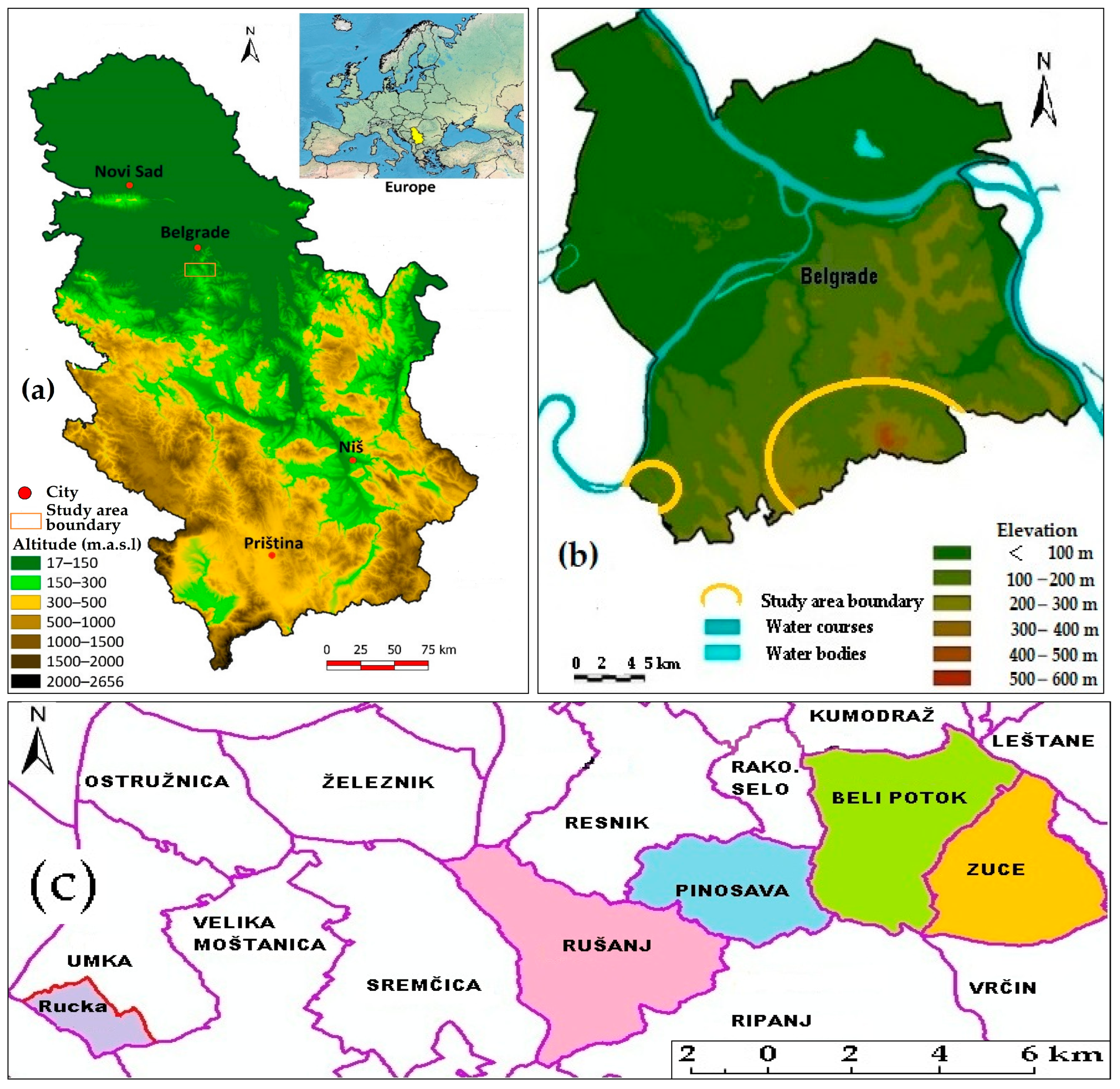
This research is focused on the advantages, disadvantages, and quality assessment mapping of soil erosion applying a GIS, without surveying. The subject of this study is the development of a soil erosion map using GIS technology according to the EPM without a field survey of erosion based solely on cartographic materials and satellite images for a part of the peri-urban area in Belgrade. The aim of this study is to assess the reliability of the mean coefficient of soil erosion in relation to the application of EPM erosion mapping procedures by statistical analysis.
This method would allow for a more convenient and standardized process of creating an erosion map; the majority of the work would be done by analysing cartographic materials and satellite images, whereas a small percentage would be done in the field. Field work would be reduced to verifying the erosion map obtained from the cartographic materials and satellite images. This map would have more accurate boundaries of the erosion areas, as the boundaries of the vegetation areas from land use, measured in ArcGIS, would be used. An erosion map properly prepared by EPM and the calculated erosion coefficients represents the basis for further calculations in which climatic factors have a direct impact on the amount of eroded sediments.

2. Research Area

The area of this research extends between the north latitudes 44°36.8′ and 44°44′ and the east longitudes 20°16′ and 20°36′. It includes suburbs located 20 km south of the centre of Belgrade. It consists of the settlements Rucka, Rušanj, Pinosava, Beli Potok, and Zuce, which belong to the hilly peri-urban area of Belgrade (Figure 1). The total area of the research area is 5687.08 ha.
Most of the territory consists of different varieties of sandstone, limestone, and carbonate rocks. These areas are subject to erosion, with visible traces of gully erosion. A smaller part of the territory, about 15%, consists of serpentines.
The average annual precipitation for the area during the period 1960–1970 was 635 mm and the air temperature was 11.7 °C. The average annual precipitation for the area between 1960 and 2018 was 675 mm and the air temperature was 12.3 °C [37].
Most soils are eutric cambisol, covering about 87% of the territory. Other types of pedological cover are humofluvisol, making up 7%, and vertisol, podzol, and chernozem, each making up 2% [38] (Table 1, map No. 3).
About 30% of the researched area is under deciduous forest vegetation and orchards, within which residential areas have been developed. The settlement of Beli Potok, located on the slopes of Avala (506 m above sea level), which is the highest point of the exploration area, has a slightly larger area under forest. The lowest point is 85 m above sea level in the village of Rucka. This area is characterised by minor areas of arable land and an increased area of fallow (abandoned) land. The valley sides gravitate towards the basins of two rivers: the Topčiderska and Bolečka. Water flows directly into the Sava River from the area around the settlement of Rucka. The southern part of the research area is furrowed with a 2–5 m deep gully. This area is characterised by a continuing increase in the number of inhabitants, which is accompanied by aggressive urbanization. The number of inhabitants increased in the period between 1971 and 2011 by 27.1%. The population belongs to the category of an old population, and the active agricultural population is constantly declining.

3. Method

To determine the average erosion coefficient, the graphical and analytical procedure of the EPM were applied in this study. Erosion maps were made by the graphical procedure without a field survey for 1970 and 2018, and based on these maps, the average erosion coefficients were calculated. For the same respective years, the average erosion coefficients were calculated according to the analytical procedure as well as the graphical procedure using the erosion maps and field survey (Table 1, maps No. 1 and 2) and the final map for 2018. Statistical analysis evaluated the reliability of the obtained erosion coefficients from the erosion maps without the field survey.

3.1. Erosion Potential Method—EPM

The erosion potential method (EPM) was developed from the Method for the Quantitative Classification of Erosion (MQCE). [10] The original method was adapted by Prof. Slobodan Gavrilović based on the field research of 17 experimental field stations set up in several regions of Yugoslavia. The regions differed in several parameters (climate, geology, soil, slopes, and relief) and visible traces of erosion. The EPM does not investigate the physics of erosion processes and, as such, is suitable for areas where there is only partial information available and no erosion research has been performed. The method is “the most quantitative of all semi-quantitative methods” [41]. The EPM can provide data on total sediment production, erosion intensity, and suspended as well as transported sediments depending on the following factors: climatological (average annual temperatures and amounts of precipitation), vegetation, land use, types of soils, relief (slope and highest and lowest points of the basin), visible traces of erosion, volume of the basin, and catchment area. The aim of this research is to make an erosion map and determine the mean erosion coefficient, which is a synthetic factor and the most influential for determining the intensity of erosion.
The annual erosion intensity according to the EPM model is estimated according to the following equation:
W y e a r = T × H y e a r × π × Z 3 × F
where:
  • Wyear is the total annual erosion (m3/year/km2).
  • T is the temperature coefficient.
  • Hyear is the average yearly precipitation (mm).
  • F is the basin area (km2) and Z is the erosion coefficient.
The temperature coefficient (T) is calculated from the following equation:
T = t 0 10 + 0.1
According to the EPM, the erosion coefficient can be determined by analytical and graphical procedures, and its value ranges from 0.01 to 1.5 for natural basins.
The analytical procedure is based on the knowledge of soil resistance, the protection of soil from the effects of the atmosphere, the visible traces of erosion, and the average inclination of the area. The analytical procedure is a numerical model of erosion that determines the average erosion coefficient of the area according to the following equation:
Z = Y X ( φ + J s r )

EPM Applied to the Study Area

The average erosion coefficients were determined by the analytical procedure for all five settlements for 1970 and 2018. The coefficients for X, Y, and φ are in Tables S1–S3. Tables S1–S4, in the supplementary file, are designed on the basis of the field and laboratory research of the experts on torrential waters and erosion in Serbia.
The value of coefficient Y is the soil erosion resistance coefficient, determined from a pedological map (Table 1, map No. 3).Y is calculated based on the established percentages of the presence of each type of land formation, multiplied by the value for that type, given in Table S1. This is the partial value of Y. Summing those partial values, one obtains the Y coefficient for the area.
The value of coefficient X is the numerical value of soil protection from atmospherics and erosion by natural conditions—vegetation and the like—and it is expressed through the way of land use, namely in the following ways:
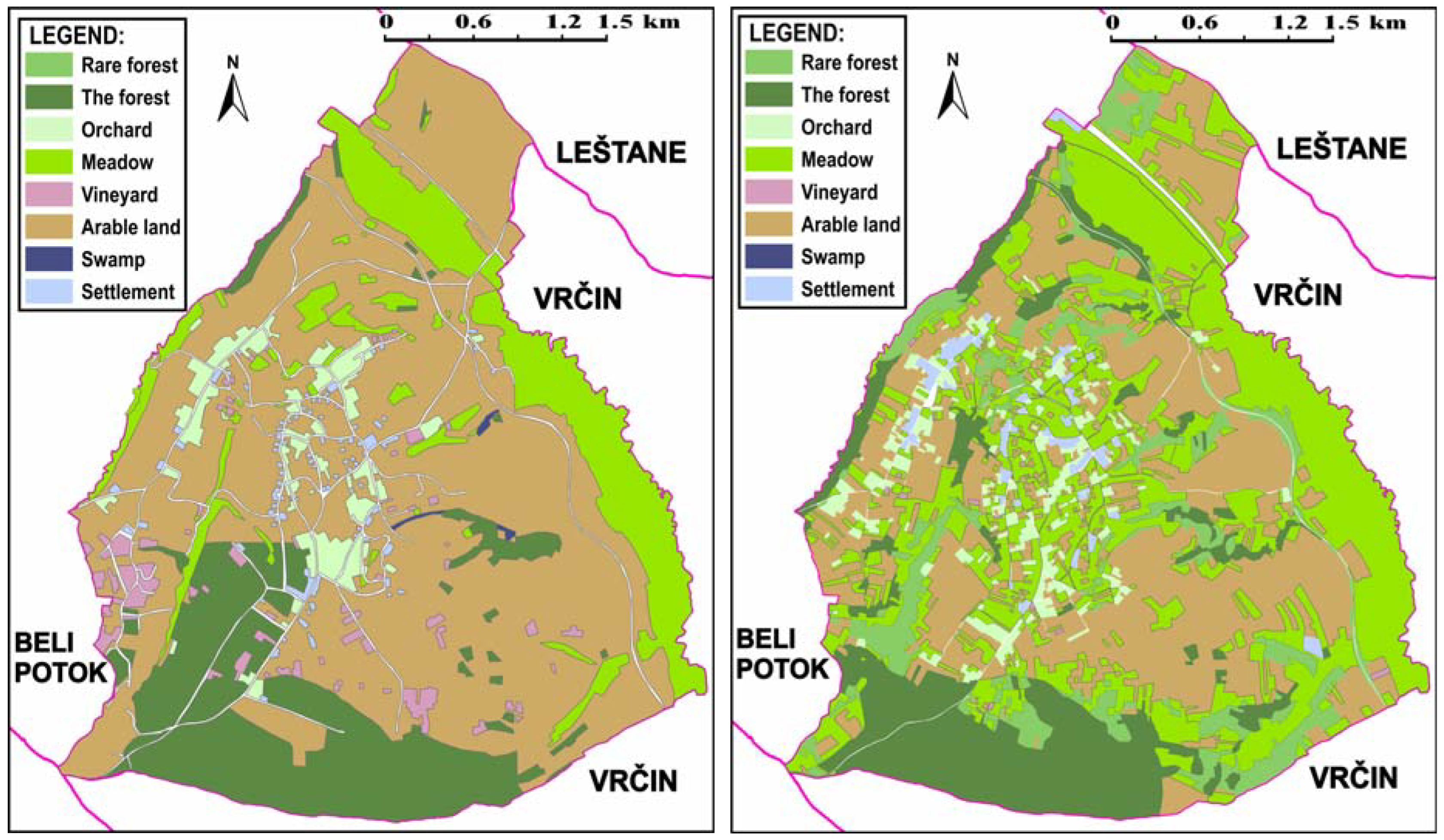
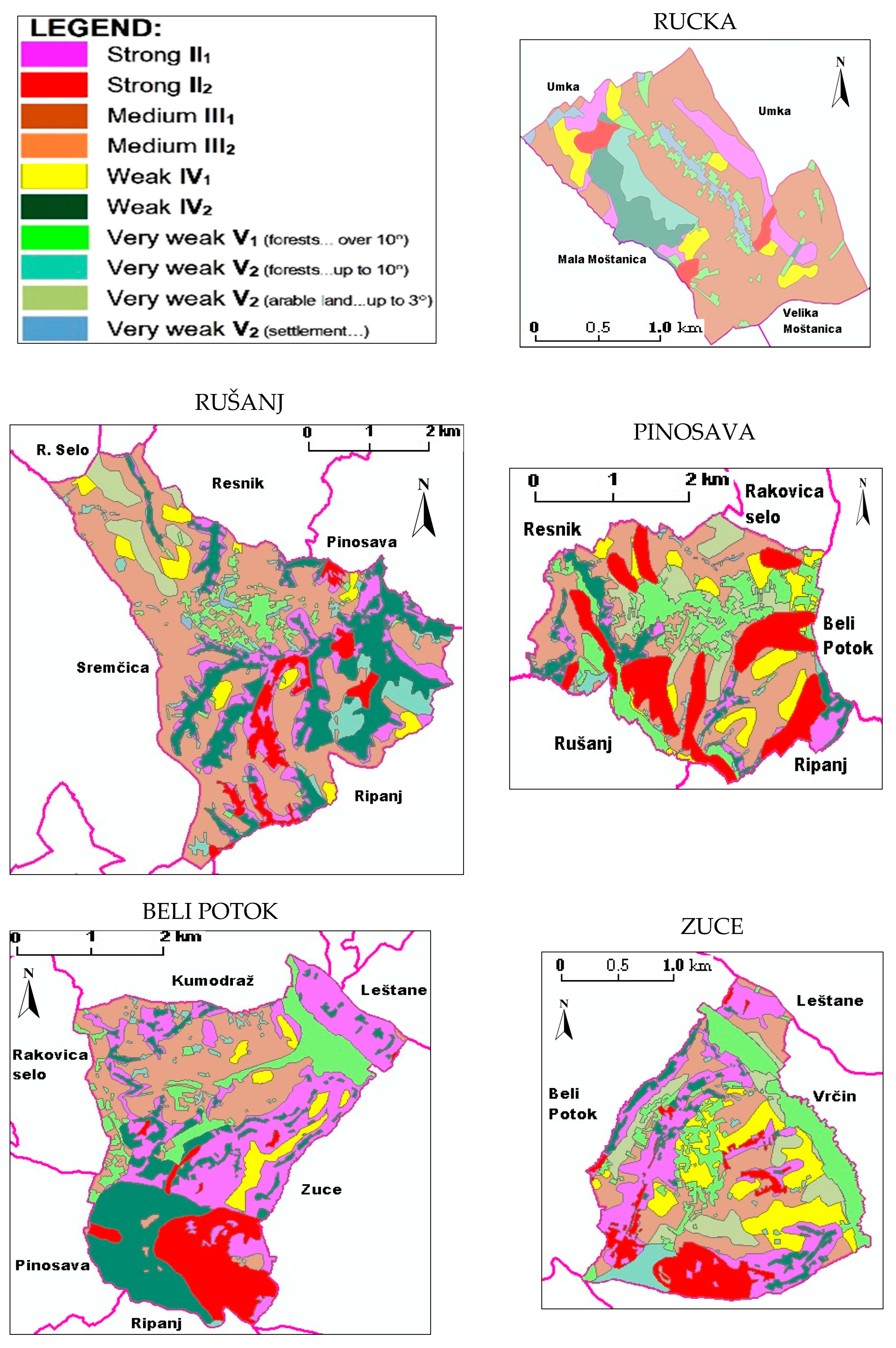
  • For 1970, X was determined based on a land-use map (Figure 2, left), which was made using a combination of maps (Table 1, maps No. 4 and 6). They were combined in order to overcome the lack of data in terms of maps, so as to generate a more accurate land-use map. Two maps were combined to avoid the disadvantages of one in relation to the other;
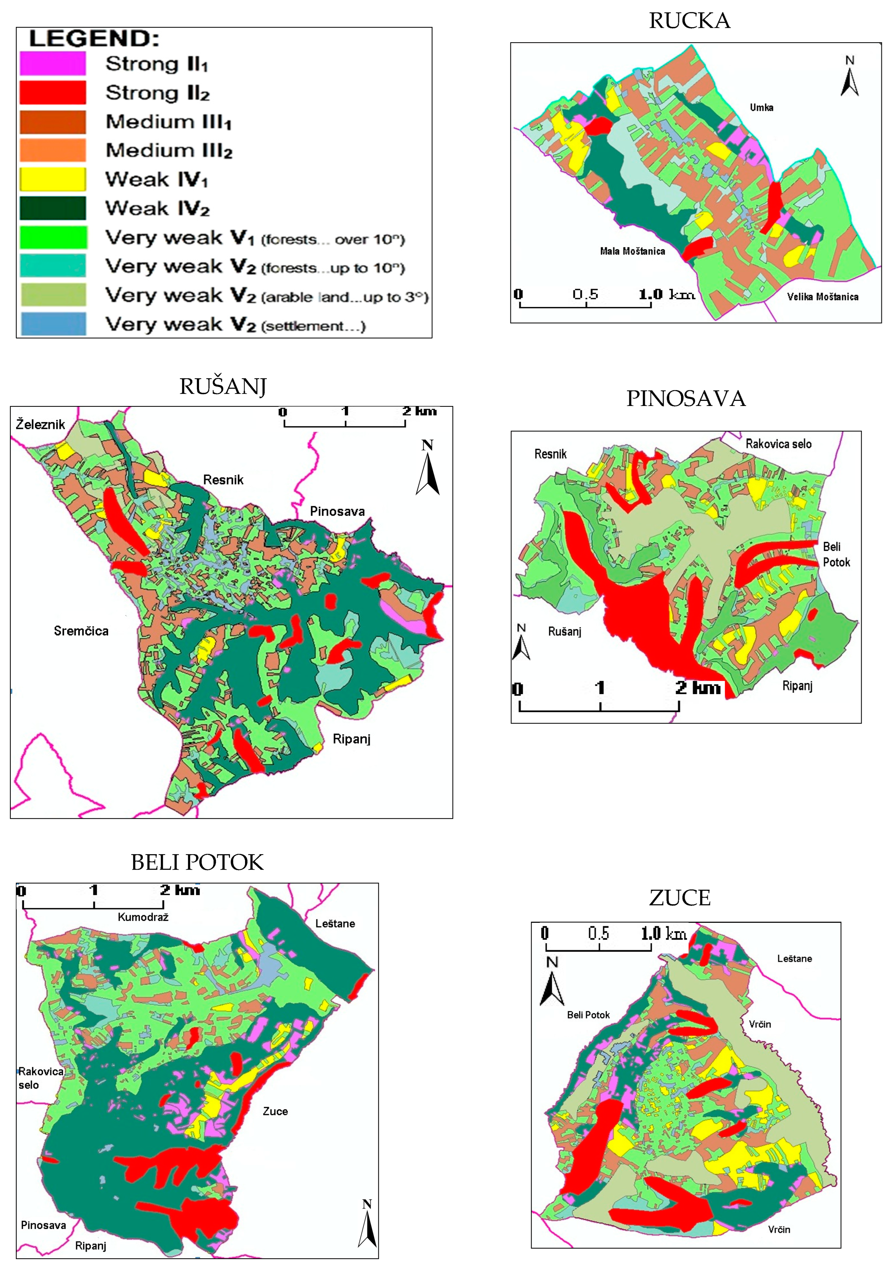
  • For 2018, the value of coefficient X was determined on the basis of a land-use map, which was made from satellite images (Table 1, No. 8).
X is calculated based on the established percentages of the presence of each land-use category multiplied by the land-use value for that type, given in Table S2. This is the partial value of X. Summing those partial values, one obtains the X coefficient for the area.
The coefficient φ is the numerical equivalent of the visible and clearly expressed erosion processes in the research area according to the following:
  • For the year 1970, coefficient φ was determined on the basis of cartographic signs on maps (Table 1, maps No. 5 and 6).
  • For the year 2018, coefficient φ was determined on the basis of cartographic signs from the map (Table 1, map No. 7) and observations directly from the site in 2018.
φ is calculated based on the percent of the representation of visible erosion traces multiplied by the value in Table S3. This is the partial value of φ. Summing those partial values, one obtains the φ coefficient for the area.
The values of coefficients X, Y, and φ are presented in Tables S1–S3, respectively. The erosion intensities, erosion categories, and ranges of Z are presented in Table S4.
The value of coefficient Jsr is the mean average slope of the area, determined by settlements based on the lengths of contours from the contents of the map (Table 1, map No. 7).
J s r = 1 F [ h 0 × L 1 2 + ( L 2 + L 3 + ..... L n 1 ) × h + h n L n 2 ]
where:
  • F = area of the settlement or territory;
  • h0 = difference between the lowest point and the first higher contour;
  • L1 = length of the contour above the lowest point;
  • L2Ln−1 = length of contours;
  • h = contour interval;
  • hn = difference between the highest point and the first lower contour;
  • Ln = length of the contour below the highest point.
The graphical procedure for determining the average erosion coefficient for an area, via the method of erosion potential, is obtained in existing maps by measuring the areas by erosion type and calculating the percent of their share in the total area. The percentage value of each erosion type is multiplied by the average erosion coefficient from Table 2, and thus one partial value of the erosion coefficient is obtained. The average erosion coefficient for the area is obtained by summing the partial values of the erosion coefficient.

3.2. Cartographic Method and Realization of an Erosion Map Using GIS Technology

The cartographic method is very common in the two procedures of the EPM model (analytical and graphical) in order to determine the average coefficient of erosion through the following procedures: planimetry, calculating a linear object’s length, and mapping. To determine the average erosion coefficient according to the analytical procedure, the following surfaces were measured by planimetry on a georeferenced map in ArcGIS: the vegetation surfaces, the categories of soil, the visible traces of erosion, and the lengths of contours.
To determine the mean erosion coefficient by the graphical procedure, the existing erosion maps (Table 1, maps No. 1 and 2) were georeferenced in ArcGIS. Considering that previous research for this area was performed in basins, it was necessary to include habitat boundaries and then calculate the areas under different types of erosion. To create a new erosion map, it was necessary to have a slope map, land cover map, and Table 2 (legend symbols for erosion types).
Land-use maps are made for each period for all five settlements as follows:
For 1970, the land-use map was made using the maps (Table 1, maps No. 4 and 6). These two maps were combined in order to avoid the flaws of one in relation to the other.
For 2018, the land-use maps were made on the basis of satellite images (Table 1, No. 8).
CORINE maps were not used because they have a high degree of generalization of spatial data [42] through five categories, from which arable areas as very important factors of erosivity are not clearly observed. For 1970, there is no possibility of its use. The mapping scale is 1:100,000 with an accuracy of not less than 100 m.
Slope maps (Figure 3) were made separately for the five locations, based on the map (Table 1, map No. 7). In Serbia, zoning is most often used in the following ranges: 0° to 3°, 3° to 5°, 5° to 10°, and more than 10°.
According to the map (Table 1, map No. 7), with the use of a slope scale, slope areas were separated. If there was no slope scale, then a graph of the function was used:
I = E × c t g α
The equation labels are the following:
I = interval line spacing between contour lines on the map, on the basis of which the slopes of the terrain sides are defined;
E = vertical distance between contour lines on a map;
ctgα = cotangent of slope angles α = 1°, 2°, 3°,....., 45°.
In the process of creating erosion maps for 1970 and 2018, the ArcGis software package was used. By overlapping the map of land use and the slope area map with adjusting the transparency of the layer, the methods of land use on different slopes can be noticed. Figure 4 clearly shows the boundaries of arable land areas located on a slope over 10°. The layer “types of erosion” is then included. In this case, it is a “Strong 1” type of erosion according to Table 2, and it is mapped. If a map of transparent material is made, then hatching marks are used for mapping. If an erosion map for any historical period is made, as is the case for 1970, then a coloured sign is used in accordance with the available sources of information on visible traces of erosion (Table 1, map No. 6), soil fertility and quality (Table 1, map No. 5), and paedology (Table 1, map No. 3).
The map of erosion for 1970 and the draft version of the erosion map on transparent material for 2018 were generated by overlapping the maps of land use and a slope map. The draft version of the erosion map on transparent material was created using hatching symbology and was a basis for the final version of the erosion map for 2018.
The draft version of the erosion map should be at the same scale as the topographic map, the land-use map, or the satellite images. Overlaying the land-use map or a satellite image with the erosion map on transparent material in the field, it could be noticed that the mismatch of agricultural or forest area borders and erosion area boundaries needed to be corrected. Based on visible erosion traces in the field, the erosion coefficient and erosion types were corrected on-site. In accordance with Table 2, corrections from the draft version of the erosion map were corrected on the final erosion map (Figure 6).
The control of the mapped content is carried out on the basis of a plan on the observed discrepancies between the sources: images taken from the Geoserbia or Google Earth platforms and the content on a topographic map at a scale of 1:25,000.
Table 2 was created as a modification of previously used legends of signs on erosion maps in the Republic of Serbia; the descriptions and ranges of the erosion coefficients by the types of erosion are shown in Table S4, based on the research in Serbia by Gavrilović [43], Lazarević [44], and Kostadinov [45].

3.3. Statistical Methods

Statistical methods were applied to determine the differences between the average erosion coefficients using arithmetic means in relation to the erosion recording methods and the recording time periods. The F-test was used to test the differences in the arithmetic means of the erosion coefficients of the methods used to determine the average erosion coefficient for 1970. The t-test was used to assess statistical differences between the relevant methods applied in one period and between two periods of erosion recording. Statistical analyses were performed in the IBM SPSS Statistics 26 software package [46].

4. Research Results

The results of the research are the erosion maps for 1970 (Figure 5) and the erosion maps for 2018 (Figure 6). For each year of the research, five erosion maps were made (one for each settlement).
For the 1970 map, there was no possibility of the field control of the mapped contents, so the maps (Table 1, maps No. 3, 5 and 6) were used for correction, respecting the note below Table 2. For 2018, when mapping using GIS technology, two maps were produced, one on the transparent paper, to control the mapped content in the field, and another map after field observations. During the land inventory, no major deviations in the erosion areas or erosion coefficients were observed.
A land inventory was performed for all five settlements in the period between April and June 2018, after which the mapping was performed. The following is an example of the results of a land inventory of the settlement of Zuce: On the map (Table 1, map No. 7) for the settlement of Zuce, a vineyard is shown when it is not in the satellite image (Table 1, No. 8) or in nature. In the southern part of the settlement of Zuce, there is a continuous forest on the Geoserbia portal, and hangars and a road network can be seen on the Google Earth website. The existence of special-purpose facilities was confirmed in the field. A meadow is shown in the northern part of the Zuce settlement, and a large complex of an “Ikea” shopping centre with a large parking facility was noticed at the spot. After the field inventory was completed, corrections were drawn and the final appearance of the erosion map was formed.
Based on the erosion maps produced by the maps and satellite images, Table 1, using GIS technology, the average erosion coefficients for each settlement were calculated for the periods 1970 and 2018 (Table 3); the arithmetic mean was calculated for the area afterwards.
By comparing the values of the arithmetic means between the two recording periods, a significant difference was noticed. The obtained values were tested by statistical analysis.
For 1970, a total of four values of the average erosion coefficient of the area was determined: one by the analytical and three by the graphical procedure. The values of the average erosion coefficient were graphically determined on the basis of erosion maps (Table 1, maps No. 1 and 2) as well as the erosion map without field observations. The analytical procedure determined the average erosion coefficient based on maps (Table 1, maps No. 3, 4, 6 and 7) as well as on land-use maps, as shown in Figure 3 (left).
For 2018, three values of the average erosion coefficient were determined: one by the analytical and two by the graphical procedure. The following were used for the analytical procedure: land-use maps (Figure 3, on the right) and maps (Table 1, maps No. 3 and 7). The value of the erosion coefficient on the draft version of the erosion map and the final erosion map was determined by the graphical procedure. Between these two maps, minimal deviations by settlement have been determined, and no significant difference between the arithmetic means was found.
Table 4 shows the values of the arithmetic means of the average erosion coefficient range obtained by the analytical procedure and the graphical procedure for both periods. To control the results of mapping based on cartographic materials and satellite images using the GIS, the areas of erosion types were measured from existing erosion maps (Table 1, maps No. 1 and 2) and maps that are necessary for determining the average erosion coefficient via the analytical procedure.

Statistical Evaluation of Results

Table 4 shows the existence of differences between the arithmetic means. The observed differences were statistically significant at p < 0.05.
The statistical analysis of the arithmetic means of the mean erosion coefficients determined by the analytical procedure for 1970 and 2018 (columns one and five of Table 4) shows that (M = 18.20, SD = 3.96); t (4) = 10.27, p = 0.001. By testing the arithmetic means of the average erosion coefficients determined from the maps obtained from the cartographic materials and satellite images for 1970 and 2018 (columns four and seven of Table 4), we discerned that (M = 17.40, SD = 4.56); t (4) = 8.53, p = 0.001.
The results obtained from the average erosion coefficient between periods by any method are statistically significant and differ from each other with a probability of more than 95%.
An analysis of four arithmetic means (columns one, two, three, and four, Table 4) using the F-test, for the period 1970, revealed that the differences in the arithmetic means of the average coefficients, compared to the method of recording erosion during 1970, are not statistically significant because (Mtot = 53.85, SDtot = 7.00); F (3, 16) = 2.39, p = 0.107. It was determined that each of the results obtained, regardless of the method, can be used in other research as well.
Using the t-test for the pairs of the arithmetic means of the average erosion coefficients, for the year 1970, the results were compared by column four with columns one and two (Table 4). The test determined that maps created on the basis of cartographic materials and satellite images have acceptable results regarding the average erosion coefficient, since the differences in the arithmetic means are not statistically significant.
By comparative analysis, for the year 2018, it was determined that the arithmetic means of the average erosion coefficients for columns six and seven are “equal”, and therefore the t-test between the two arithmetic means between columns five and seven was applied. It was found that there was no statistically significant difference between the arithmetic means of the average erosion coefficients because (M = −0.60, SD = 4.83); t (4) = −0.28, p = 0.795.
The results obtained within either 1970 or 2018, regardless of the method of determining the average erosion coefficient, have no statistically significant difference. This was determined with a probability of more than 95%.

5. Discussion

Prior to the development of a GIS, erosion mapping required extensive field work and highly trained personnel, who would assess the terrain slope, observe erosion patterns and the types of vegetation, and, based on knowledge of the geology of the land, determine the erosion coefficient according to Tables S1–S3. This way of working contained a lot of subjective assessments and required personnel who had the same criterion for evaluating erosive surfaces in the field.
The process of mapping erosion using cartographic materials, satellite images, and GIS technology is a specific graphical procedure. In this research, that procedure was used to create an erosion map for the year 1970, as well as for 2018. The precondition for making an erosion map for those years is to already have a land-use map and relief slope map for the area. If a relief slope map is not obtainable, it is necessary to have a map showing the relief by contours in order to produce a relief slope map. If a land-use map is not available for a certain period, it is necessary to have adequate topographic maps, such as maps and satellite images (Table 1, maps No. 4, 6 and 7 and satellite images No. 8), or aerial photographs. Topographic maps (Table 1, maps No. 6 and 7) are good indicators of the visible traces of erosion that are difficult to detect in satellite images and aerial photos.
The erosion map for the current period should be constructed in two phases: First, the erosion map on the transparent paper is made, where the erosion area is presented by hatching symbology. Field corrections and erosion coefficients are entered into the map from field observations, and then in the second phase, using GIS, these field corrections are entered into the final erosion map. This procedure is called research center-field-research center.
This research shows that the erosion coefficient obtained from the erosion map, made without visually verifying the site, is statistically acceptable. The accuracy of the presented contents is higher because the process is performed on the basis of the proportional and instrumentally determined boundaries of land use and clearly defined slope area.
The process of mapping, based on cartographic materials and satellite images, has a number of significant positive outcomes, including the following: the time required for field work is reduced, causing a subsequent reduction in erosion map production costs; preparations for field trips can be more comprehensive; projects are easier to implement by understanding erosion hazards and investment risks for projects; and proposals for anti-erosion measures are easier to define. Field checking is focused on critical and unclear erosion areas that are assessed using cartographic materials, so the situation is verified on the terrain and necessary anti-erosion measures are proposed.
Over 80% of the mapping of erosion areas can be completed based on cartographic materials and satellite images. The production of a draft version of a map can be performed by professionals who might not be experts in calculating erosion (technical personnel) as a preparatory document for the inventory of a study area. Field observations can be performed by students of forestry, geography, agriculture, construction engineering, etc., i.e., persons trained in identifying the visible traces of erosion. In observing the terrain, land use should be identified, such as arable land, forests, pastures, vineyards, etc., as should the visible traces of erosion; in accordance with the observations, erosion boundaries and coefficients should be corrected.
The draft version of an erosion map can be used in public discussions when proposing projects of anti-erosion measures and making a final erosion map of an area.
The weakness of the method lies in the dependency on reliable cartographic sources and aerial and satellite images. Making historical erosion maps using this method would depend on available sources for that period of time.

6. Conclusions

The research clearly indicated that, with the help of high-quality large-scale topographic maps and adequate aerial imaging, mapping can be successfully performed as preparation for field work or the production of broad-scale erosion maps for any historical period.
Creating a map based on cartographic materials and satellite images without field observation, it is possible to assess soil losses in previous periods and create a draft version of the map for the field observations of erosion. Based on obtained mean erosion coefficients and climatological factors, soil losses (Wsp) were calculated, amounting to 10.64 t ha−1 year−1 in 1970 and 5.79 t ha−1 year−1 in 2018.
A detailed analysis of anthropogenic factors on the intensity of erosion determined that in the period from 1970 to 2018 there was a decrease in arable land (by 59.7%) and livestock (by 42.4%). In the same period, there was an increase in the areas of forest (by 37.6%), meadows (by 219.3%), and infrastructure facilities (by 56.8%).
The results obtained using statistical analysis (arithmetic means) indicate that the value of the average erosion coefficient obtained by the cartographic materials and satellite images does not statistically differ from the results obtained by graphical and analytical procedures.
Statistical analysis (F-test) proved that the obtained value of the coefficient of erosion from cartographic materials and satellite images without going to the field is reliable, compared to the values obtained by other methods (Table 4) for 1970 and 2018. Statistical analysis (t-test) showed a decrease in the value of the erosion coefficient from 1970 to 2018, regardless of the method applied.
The assumptions in this study have been tested experimentally by processing measurable cartographic and aerial photo documentation and should be understood as conceptual for the application of this research in other geographical areas, especially in areas with excessive erosion. We feel that it would be a good idea to compare the results with detailed field measurements, but there are no data for our study area at this time.

Supplementary Materials

The following supporting information can be downloaded at: https://www.mdpi.com/article/10.3390/land11071096/s1, Table S1. Conditions affecting the value of coefficient Y; Table S2 Conditions affecting the value of coefficient X; Table S3 Conditions affecting the value of coefficient φ; Table S4 Erosion intensity, erosion category, and range of erosion coefficient.

Author Contributions

Conceptualization, N.V.; methodology, N.V. and M.T.; validation, N.V., M.T. and D.Š.; formal analysis, N.V. and D.Š.; writing—original draft preparation, N.V.; writing—review and editing, M.T. and D.Š. All authors have read and agreed to the published version of the manuscript.

Funding

This research received no external funding.

Institutional Review Board Statement

Not applicable.

Informed Consent Statement

Not applicable.

Data Availability Statement

The data presented in this study are available on request from the corresponding author.

Conflicts of Interest

The authors declare no conflict of interest.

References

  1. Benavidez, R.; Jackson, B.; Maxwell, D.; Norton, K. A review of the (Revised) Universal Soil Loss Equation (R/USLE): With a view to increasing its global applicability and improving soil loss estimates. Hydrol. Earth Syst. Sci. 2018, 22, 6059–6086. [Google Scholar] [CrossRef] [Green Version]
  2. Fan, X.; Scaringi, G.; Korup, O.; West, A.J.; van Westen, C.J.; Tanyas, H.; Hovius, N.; Hales, T.C.; Jibson, R.W.; Allstadt, K.E.; et al. Earthquake-induced chains of geologic hazards: Patterns, mechanisms, and impacts. Rev. Geophys. 2019, 57, 421–503. [Google Scholar] [CrossRef] [Green Version]
  3. Samaras, A.G.; Koutitas, C.G. The impact of watershed management on coastal morphology: A case study using an integrated approach and numerical modeling. Geomorphology 2014, 211, 52–63. [Google Scholar] [CrossRef]
  4. Petrović, A.M. Challenges of torrential flood risk management in Serbia. J. Geogr. Inst. Jovan Cvijic SASA 2015, 65, 131–143. [Google Scholar] [CrossRef]
  5. Wischmeier, W.H.; Smith, D.D. Predicting Rainfall-Erosion Losses—A Guide to Conse-Rvation Planning; Agriculture Handbook No. 537; U.S. Department of Agriculture: Washington, DC, USA, 1978; p. 58. Available online: https://naldc.nal.usda.gov/download/CAT79706928/PDF (accessed on 20 March 2022).
  6. Renard, K.; Foster, G.R.; Weesies, G.A.; McCool, D.K.; Yoder, D.C. Predicting Soil Erosion by Water: A Guide to Conservation Planning with the Revised Universal Soil Loss Equation (RUSLE); Agricultural handbook No. 703; U.S. Department of Agriculture: Washington, DC, USA, 1997; p. 407. ISBN 0-16-048938-5. [Google Scholar]
  7. Kirkby, M.J.; Irvine, B.J.; Jones, R.J.A.; Govers, G.; Boer, M.; Cerdan, O.; Daroussin, J.; Gobin, A.; Grimm, M.; Le Bissonnais, Y.; et al. The PESERA coarse scale erosion model for Europe. I.—Model rationale and implementation. Eur. J. Soil Sci. 2008, 59, 1293–1306. [Google Scholar] [CrossRef]
  8. Karydasa, G.C.; Panagos, P. The G2 erosion model: An algorithm for month-time step assessments. Environ. Res. 2018, 161, 256–267. [Google Scholar] [CrossRef]
  9. Morgan, R.P.C.; Quinton, J.N.; Smith, R.E.; Govers, G.; Poesen, J.W.A.; Auerswald, K.; Chisci, G.; Torri, D.; Styczen, M.E. The European Soil Ersoion Model (EUROSEM): A dynamic approach for predicting sediment transport from fields and small catchments. Earth Surf. Processes Landf. 1998, 23, 527–544. [Google Scholar] [CrossRef]
  10. Gavrilovic, Z.; Stefanovic, M.; Milovanovic, I.; Cotric, J.; Milojevic, M. Torrent classification—Base of rational management of erosive regions. IOP Conf. Ser. Earth Environ. Sci. 2008, 4, 012039. [Google Scholar] [CrossRef]
  11. Gavrilovic, Z.; Stefanovic, M.; Milojevic, M.; Cotric, J. Erosion Potential Method An Important Support For Integrated Water Resource Management. Inst. Dev. Water Resour. Jaroslav Cerni 2004, 1–14. Available online: https://balwois.com/wp-content/uploads/old_proc/ffp-700.pdf (accessed on 10 January 2022).
  12. Dragičević, N.; Karleuša, B.; Ožanić, N. A review of the Gavrilović method (erosion potential method) application. Građevinar 2016, 68, 715–725. [Google Scholar] [CrossRef]
  13. Batista, P.V.G.; Davies, J.; Silva, M.L.N.; Quinton, J.N. On the evaluation of soil erosion models: Are we doing enough? Earth-Sci. Rev. 2019, 197, 102898. [Google Scholar] [CrossRef]
  14. Igwe, P.U.; Onuigbo, A.A.; Chinedu, O.C.; Ezeaku, I.I.; Muoneke, M.M. Soil Erosion: A Review of Models and Applications. Int. J. Adv. Eng. Res. Sci. 2017, 4, 237341. [Google Scholar] [CrossRef]
  15. Perović, V. Assessment of Soil Erosion Potential by Application of USLE and PESERA Models on the Territory of Prvonek Catchment. Ph.D. Thesis, University of Belgrade, Belgrade, Serbia, July 2015. (In Serbian). [Google Scholar]
  16. Alewell, C.; Borrelli, P.; Meusburger, K.; Panagos, P. Using the USLE: Chances, challenges and limitations of soil erosion modelling. Int. Soil Water Conserv. Res. 2019, 7, 203–225. [Google Scholar] [CrossRef]
  17. Blinkov, I. The Balkans—The most erosive part of Europe? Glasnik Sumarskog Fakulteta 2015, 111, 9–20. [Google Scholar] [CrossRef] [Green Version]
  18. Spalevic, V.; Barović, G.; Vujačić, D.; Curović, M.; Behzadfar, M.; Djurović, N.; Dudić, B.; Billi, P. The Impact of Land Use Changes on Soil Erosion in the River Basin of Miocki Potok, Montenegro. Water 2020, 12, 2973. [Google Scholar] [CrossRef]
  19. Oltion, M.; Gjipalaj, J.; Shkodrani, N. Application of the Erosion Potential Method in Vithkuqi Watersheds (Southeastern Albania). J. Ecol. Eng. 2022, 23, 17–24. [Google Scholar] [CrossRef]
  20. Gocić, M.; Dragićević, S.; Radivojević, A.; Bursać, M.N.; Stričević, L.j.; Đorđević, M. Changes in Soil Erosion Intensity Caused by Land Use and Demographic Changes in the Jablanica River Basin Serbia. Agriculture 2020, 10, 345. [Google Scholar] [CrossRef]
  21. Lovrić, N.; Tošić, R. Assessment of soil erosion and sediment yield using erosion potential method: Case study—Vrbas river basin (B&H). Bull. Serb. Geogr. Soc. 2018, 98, 1–14. [Google Scholar] [CrossRef]
  22. Elhag, M.; Kojchevska, T.; Boteva, S. EPM for Soil Loss Estimation in Different Ge- omorphologic Conditions and Data Conversion by Using GIS. IOP Conf. Ser. Earth Environ. Sci. 2019, 221, 012079. [Google Scholar] [CrossRef]
  23. Efthimiou, N.; Lykoudi, E. Soil erosion estimation using the EPM model. Bull. Geol. Soc. Greece 2016, 50, 305–314. [Google Scholar] [CrossRef] [Green Version]
  24. Emmanouloudis, D.; Christou, O.; Filippidis, E. Quantitative estimation of degradation in the Aliakmon River basin using GIS, Erosion Prediction in Ungauged Basins: Integrating Methods and Techniques. In Proceedings of the Symposium HS01, Sapporo, Japan, 7–11 July 2003; IAHS Publisher: Wallingford, UK, 2003; pp. 234–240. Available online: https://iahs.info/uploads/dms/12639.34-234-240--HS1-24-Emmanouloudis-et-al.pdf (accessed on 20 January 2022).
  25. Aristeidis, K.; Vasiliki, K. Influence of Land Use Changes on Alluviation of Volvi Lake Wetland (North Greece). Soil Water Res. 2015, 10, 121–129. [Google Scholar] [CrossRef] [Green Version]
  26. Berteni, F.; Grossi, G. Water Soil Erosion Evaluation in a Small Alpine Catchment Located in Northern Italy: Potential Effects of Climate Change. Geosciences 2020, 10, 386. [Google Scholar] [CrossRef]
  27. Zorn, M.; Komac, B. Response of soil erosion to land use change with particular reference to the last 200 years (Julian Alps, Western Slovenia). In Proceedings of the IAG Regional Conference on Geomorphology: Landslides, Floods and Global Environmental Change in Mountian Regions, Brasov, Romania, 15–25 September 2008; pp. 39–47. Available online: https://www.geomorfologie.ro/wp-content/uploads/2015/07/Revista-de-geomorfologie-nr.-11-2009-05.zorn_.pdf (accessed on 20 January 2022).
  28. Globevnik, L.; Holjević, D.; Petkovšek, G.; Rubinić, J. Applicability of the Gavrilović method in erosion calculation using spatial data manipulation techniques; Erosion Prediction in Ungauged Basins: Integrating Methods and Techniques. In Proceedings of the Symposium HS01, Sapporo, Japan, 7–11 July 2003; IAHS Publisher: Wallingford, UK, 2003; pp. 224–233. Available online: https://www.researchgate.net/publication/242554907_Applicability_of_the_Gavrilovic_method_in_erosion_calculation_using_spatial_data_manipulation_techniques (accessed on 23 February 2022).
  29. Kouhpeima, A.; Hashemi, A.A.; Feiznia, S. A study on the efficiency of Erosion Potential Model (EPM) using reservoir sediments. Elixir Pollut. 2011, 38, 4135–4139. Available online: https://www.researchgate.net/publication/261875115_A_study_on_the_efficiency_of_Erosion_Potential_Model_EPM_using_reservoir_sediments (accessed on 5 February 2022).
  30. Tabarestani, E.S.; Afzalimehr, H.; Sui, J. Assessment of Annual Erosion and Sediment Yield Using Empirical Methods and Validating with Field Measurements—A Case Study. Water 2022, 14, 1602. [Google Scholar] [CrossRef]
  31. Zahnoun, A.; Makhchane, M.; Chakir, M.; Karkouri, J.; Watfae, A. Estimation and cartography the water erosion by integration of the Gavrilovic “EPM” model using a GIS in the Mediterranean watershed: Lower Oued Kert watershed (Eastern Rif, Morocco). Int. J. Adv. Res. Ideas Innov. Technol. 2019, 5, 367–374. [Google Scholar]
  32. Poggetti, E.; Cencetti, C.; De Rosa, P.; Fredduzzi, A.; Rivelli, R.F. Sediment Supply and Hydrogeological Hazard in the Quebrada De Humahuaca (Province of Jujuy, Northwestern Argentina)—Rio Huasamayo and Tilcara Area. Geosciences 2019, 9, 483. [Google Scholar] [CrossRef] [Green Version]
  33. Stefanović, M.; Gavrilović, Z.; Bajčetić, M. Local Communities and Challenges of Torrential Floods; Organization for Security and Co-operation in Europe, Mission to Serbia: Belgrade, Serbia, 2004; pp. 12–18. Available online: https://www.osce.org/sr/serbia/148311 (accessed on 23 March 2022).
  34. Smailagić, J.; Savović, A.; Marković, D.; Nešić, D.; Drakula, B.; Milenkovic, M.; Zdravkovic, S. Climate Characteristics of Serbia; Republic Hydrometeorological Service of Serbia: Belgrade, Serbia, 2013; pp. 1–26. Available online: https://www.hidmet.gov.rs/data/klimatologija_static/eng/Klimatske_karakteristike_Srbije_prosirena_verzija.pdf (accessed on 28 April 2022). (In Serbian)
  35. Institute for Water Management “Jaroslav Černi”. Plan for the Proclamation of Erosion Areas for the Area of the City of Belgrade; Faculty of Forestry, Department of Torrents and Erosion Belgrade, Administration of the City of Belgrade: Belgrade, Serbia, 2005. (In Serbian) [Google Scholar]
  36. Dragićević, S.; Stepić, M. Changes in the intensity of erosion in the Ljig basin—The impact of anthropogenic factors. Gaz. Serb. Geogr. Soc. 2006, 86, 37–44. [Google Scholar]
  37. Republic Hydrometeorological Service of Serbia. Available online: https://www.hidmet.gov.rs/latin/meteorologija/klimatologija_godisnjaci.php (accessed on 8 April 2019). (In Serbian)
  38. FAO. World Reference Base for Soil Resources 2014, International Soil Classification System for Naming Soils and Creating Legends for Soil Maps, Update 2015. Available online: https://www.fao.org/3/i3794en/I3794en.pdf (accessed on 29 June 2022).
  39. Valjarević, A.; Morar, C.; Živković, J.; Niemets, L.; Kićović, D.; Golijanin, J.; Gocić, M.; Bursać, N.M.; Stričević, L.; Žiberna, I.; et al. Long Term Monitoring and Connection between Topography and Cloud Cover Distribution in Serbia. Atmosphere 2021, 12, 964. [Google Scholar] [CrossRef]
  40. Pecelj, M.; Matzarakis, A.; Vujadinović, M.; Radovanović, M.; Vagić, N.; Đurić, D.; Cvetkovic, M. Temporal Analysis of Urban-Suburban PET, mPET and UTCI Indices in Belgrade (Serbia). Atmosphere 2021, 12, 916. [Google Scholar] [CrossRef]
  41. DeVente, J.; Poesen, J. Predicting soil erosion and sediment yield at the basin scale: Scale issues and semi-quantitative models. Earth-Sci. Rev. 2005, 71, 95–125. [Google Scholar] [CrossRef]
  42. Polovina, S.; Radić, B.; Ristić, R.; Kovačević, J.; Milčanović, V.; Živanović, N. Soil Erosion Assessment and Prediction in Urban Landscapes: A New G2 Model Approach. Appl. Sci. 2021, 11, 4154. [Google Scholar] [CrossRef]
  43. Gavrilović, S. Engineering of Torrents Flows and Erosion; Publisher Izgradnja, Special Edition: Belgrade, Serbia, 1972; pp. 66–82. (In Serbian) [Google Scholar]
  44. Lazarević, R. Experimental Research of Water Erosion Intensity; Torrent Association of Serbia and Montenegro: Belgrade, Serbia; Želnid: Belgrade, Serbia, 2004; pp. 204–211. (In Serbian) [Google Scholar]
  45. Kostadinov, S. Torrents and Erosion; Faculty of Forestry, University of Belgrade: Belgrade, Serbia, 2008; pp. 211–213, 317–319. (In Serbian) [Google Scholar]
  46. Coakes, J.S. SPSS Version 20.0 for Windows: Analysis without Anguish; Wiley Publishing, Inc.: Hoboken, NJ, USA, 2013; pp. 77–92. [Google Scholar]
Figure 1. The geographical position of the research area: relief map of Serbia (a) [39], relief map of Belgrade (b) [40], and study area boundary (5 settlements) (c).
Land 11 01096 g001
Figure 2. Example of land-use maps for 1970 (left) and 2018 (right) for the settlement of Zuce.
Land 11 01096 g002
Figure 3. Example of a terrain slope map for the settlement of Zuce.
Land 11 01096 g003
Figure 4. Example of the overlapping of the map of land use and the slope map for erosion mapping, for the settlement of Zuce for the year 2018.
Land 11 01096 g004
Figure 5. Erosion maps made by the graphical procedure without field observations for 1970 for the settlements Rucka, Rušanj, Pinosava, Beli Potok, and Zuce. Erosion categories and coefficients are listed in Table S4.
Land 11 01096 g005
Figure 6. Erosion maps made after the corrections were entered from the field for 2018 for the settlements Rucka, Rušanj, Pinosava, Beli Potok, and Zuce. Erosion categories and coefficients are listed in Table S4.
Land 11 01096 g006
Table 1. Maps and satellite images.
No.MapScaleSourceYear
1.Erosion map1:100,000Institute of Forestry and Wood Industry, Belgrade, Serbia.1970
2.Map of soil endangerment by erosion and water1:20,000Institute for Cartography “Geokarta”, Republic Geodetic Authority, Belgrade, Serbia.1970
3.Pedological map1:20,000
4.Land use map1:20,000
5.Map of soil fertility and quality1:20,000
6.Topographic map1:25,000Military Geographical Institute, Belgrade, Serbia.1970
7.Topographic map1:25,0001990
8.Satellite images, Belgrade “GeoSrbija”, Republic Geodetic Authority, Serbia.2013–2015
Table 2. Legend symbols for erosion types for the draft version of the erosion map and the final erosion map.
Erosion TypeErosion ClassErosion CoefficientErosion Indicators in Relation to Land Use and SlopeLegend for the
Draft Version of the Erosion Map
Legend for the Final Erosion Map
ExcessiveI11.5Surfaces furrowed by numerous gullies and landslide processes—deep erosionN/AN/A
I21.3Heavily crumbled non-resistant rocks, scree, and scree slopesN/AN/A
I31.1Of the territory, 80% under furrowed and gully erosionN/AN/A
StrongII10.9Arable land, gardens, and vineyards in the erosion area of an average incline of over 10° Land 11 01096 i001
II20.8Forests, orchards, vineyards, pastures, and meadows on eroded areas with occasionally seen gullies, ravines, furrows, landslides, and scree, regardless of the slope of the terrain Land 11 01096 i002
MediumIII10.6Arable land, gardens, and vineyards in the erosion area of an average incline of 5–10° Land 11 01096 i003
III20.5Heavily degraded pastures, sparse forests, and forests with damaged carpet on an erosive area with an average slope of 5–10° Land 11 01096 i004
WeakIV10.4Arable land, gardens, and vineyards on an incline of 3–5° Land 11 01096 i005
IV20.3Sparse forests and orchards, degraded meadows, and pastures on a slope of an average inclination of over 10° Land 11 01096 i006
Very weakV10.2Good-density forests (dense and moderately dense) and good orchards, meadows, and pastures on slopes of over 10° Land 11 01096 i007
V20.1Forests of good cover and good orchards, meadows, and pastures on slopes up to 10° Land 11 01096 i008
V2Arable land, in an erosion area with an average inclination of up to 3°, and plains with preserved vegetation (meadows and pastures) Land 11 01096 i009
V2Groups of buildings or settlements on slopes up to 10° if the buildings are not surrounded by an orchard or a forest, after which it is then mapped as a forest or orchard Land 11 01096 i010
Table 3. Average erosion coefficient values by settlement.
SettlementPeriod
Without Field ObservationsWith Field
Observations
1970Draft
Version of the 2018
Erosion Map
Final 2018 Erosion
Map
Rucka0.490.340.33
Rušanj0.490.310.31
Pinosava0.480.330.34
Beli Potok0.580.320.33
Zuce0.490.360.35
Arithmetic mean0.5060.3320.332
Table 4. Arithmetic means of the average erosion coefficients obtained by different methods for the two periods (1970 and 2018).
19702018
1234567
AnalyticalErosion map
1:100,000
1:100,000
Erosion map
1:20,000
Erosion map
without field observations
1:25,000
AnalyticalDraft version of the erosion map 1:25,000Final erosion map
1:25,000
0.5080.6000.5400.5060.3260.3320.332
Publisher’s Note: MDPI stays neutral with regard to jurisdictional claims in published maps and institutional affiliations.

