Cropland Exposed to Drought Is Overestimated without Considering the CO₂ Effect in the Arid Climatic Region of China

Abstract

Drought seriously restricts people’s lives and social–economic development. An accurate understanding of the evolution of drought characteristics and future changes in cultivated land exposure can reduce the risk of drought. There is evidence that increased CO₂ concentrations alter the physiological properties of vegetation and, thus, affect drought evolution. In this study, both changes and differences in drought (i.e., characteristics and cropland exposure) with and without the CO₂ effect over the arid region of China are investigated, using seven CMIP6 outputs and land-use under seven shared-socioeconomic-pathway (SSP)-based scenarios. The results show that: (1) drier conditions will be more severe in 2015–2100 under SSP5-8.5, especially if the CO₂ effect is neglected. Moreover, the CO₂ effect will increase with increasing emission concentrations; (2) drought intensity will be greater than in the baseline period (1995–2014, approximately −1.45) but weaker than that without the CO₂ effect under all scenarios; (3) drought frequency will decrease, and will generally decline faster if the CO₂ effect is not considered; (4) drought duration will increase and the difference between the presence and absence of the CO₂ effect will always be smallest under SSP1-1.9 and largest under SSP5-8.5; (5) drought acreage will also increase, and neglecting the CO₂ effect is always higher than that considering CO₂. The difference between the two algorithms will increase with time; and (6) cropland exposure to drought will increase, and can even reach 669,000 km² and 524,000 km² considering and ignoring the CO₂ effect, respectively. Our findings suggest that ignoring CO₂ in drought evaluations will result in significant overestimations of drought projections.

1. Introduction

Drought is one of the most common, frequent and costly natural disasters in the world, defined as below-normal precipitation lasting for a period of months to years [1,2,3]. It occurs in all climate zones, whether in tropical rainforests or deserts [4,5], due to nonperiodic climatic anomalies, and severely impacts the social economy, water resources and natural environment [6,7]. The observed increase in the frequency, intensity and severity of droughts has heightened the risk to food security, with broad and pervasive impacts on ecosystems, people, settlements and infrastructure [8,9]. Global warming, brought about by rising concentrations of greenhouse gases, may be an important reason for the increase and intensification of droughts in many regions [10,11,12,13]. The global surface temperature in the first 20 years of the 21st century (2001–2020) is reported to have been approximately 1 °C higher than that in 1850–1900 [14]. Global warming is likely to continue, which means that people will be at greater risk of drought [15,16]. Therefore, it is necessary to investigate the spatiotemporal statistical features of droughts under ongoing climate change, and address the harmful effects of rising drought risks [17]. Additionally, assessing the risk of future cropland exposure to drought is critical for climate change adaptation and disaster mitigation.

Drought evaluation, including monitoring, forecasting and projection, is generally quantified and described through some relative measures [18,19]. In addition, because total water resources and photosynthetic efficiency are strongly limited by the evaporation environment and precipitation, the most efficient way to quantify drought from climate data requires a combination of precipitation and potential evapotranspiration (PET) [20]. Precipitation is easily obtained by observation, while PET can be seen as the rate at which evapotranspiration occurs when the surface is well supplied with water [21]; PET cannot be obtained directly and is often estimated by theoretical formulas based on other meteorological data [22]. Hence, the estimation of PET can be a potential source of uncertainty in atmospheric water demands and drought [6,11,23,24], which can lead to an over- or underestimation of drought risk. The Penman–Monteith (PM) formula [25] is considered a better method for estimating PET; it combines the aerodynamic and energy terms [18,26,27], and more comprehensively considers factors affecting PET. However, Milly and Dunne (2016) [21] and Yang et al. (2019) [28] reported that the PM method will overestimate PET under increased global mean CO₂ conditions (RCP 8.5) in the future warming period. They argue that the PM formula does not take into account the implicit assumption that surface resistance (resistance to vapour flow through stomata openings) is constant with CO₂ due to changes in transpiration caused by the plant’s physiological response to increased CO₂ [29,30,31,32]. There is evidence that high concentrations of CO₂ can cause partial stomatal closure in vegetation and reduce stomatal conductance, and the increase in CO₂ concentration will increase the atmospheric pressure difference and affect stomatal opening, thus inhibiting evapotranspiration [30,33,34,35]. Thus, it is most important to have detailed information on how CO₂ inclusion will influence the changes in future drought and cropland exposure.

The overwhelming societal impacts of intense drought have drawn the utmost attention worldwide [36,37]. Drought-induced water shortages are one of the main obstacles to agricultural transformation and rural revitalization in the arid region of China. The quantitative evaluation of regional drought is of great significance for regional drought risk assessment [38]. Due to the continental climate characteristics of the arid region, precipitation is low, and river runoff mainly depends on snow and ice melt-water [39]. Agricultural development is, consequently, based mostly on irrigation. In recent years, agricultural water consumption in the arid region has increased greatly, and water resource management is facing severe challenges. Numerous studies have emphasized the evolution of prospective changes in drought over the arid region of China using various metrics and methods. In general, from the 1960s to the 2010s, climate conditions in the arid region of China tended to become more humid [40,41,42,43], but conditions will become drier in the future, according to simulations [44,45]. However, negligible effort has been exerted to explore the influence of increased CO₂ concentrations on drought characteristics over the arid region of China; in addition, an understanding of the CO₂ effect on cropland exposure is still lacking. In this paper, Global Climate Model (GCM) outputs from the sixth phase of the Coupled Model Intercomparison Project (CMIP6) and dynamic projections of land use under the seven Shared-Socioeconomic-Pathway (SSP)-based scenarios are applied to analyse the drought characteristics and cropland exposure, under the conditions of the presence and absence of the CO2 effect, during three defined future periods (near-term (2021–2040), mid-term (2041–2060), and long-term (2081–2100)). The consideration of the modified PET approach with the updated CO₂ data in this paper will provide more reasonable and reliable results.

2. Data and Methods

2.1. Study Area

The arid region of China, which is located at 30–50° N, 73–109° E, is the focus of this research, and the area accounts for approximately 30% of the total Chinese land area (Figure 1). The arid region is defined mainly by the distribution of annual precipitation, which is less than 200 mm. The arid region lies deep inland and is scarcely affected by monsoons, and the high Tibetan Plateau to the south blocks moisture from the Indian Ocean. The climate has the characteristics of low precipitation but large variability, large diurnal and annual temperature ranges, much more potential evaporation than precipitation, more sand, fewer clouds, and strong sunshine. It is also the production base of melons and other fruits, wheat, corn, cotton and cereals, as well as livestock products. Because it is a sensitive region, water resources are the main limiting factor for its development; additionally, the alteration in regional water resources due to climate change and other factors will severely impact the food security and environment in the area, which will restrict its sustainable development. Climate change has intensified the conflict between human development and environmental protection. Effective water resource management can balance the conflict between the human demand for water and environmental protection.

2.2. Datasets

In this study, meteorological observation data were collected from the National Meteorological Information Center of the China Meteorological Administration. The data included precipitation, average temperature, maximum temperature, minimum temperature, relative humidity, precipitation, air pressure, sunshine duration and other factors, at 2479 meteorological stations across China, with a daily temporal resolution and a time span of 1961–2020. After data quality control and outlier tests (such as high and low anomalies, temporal anomalies and spatial anomalies), the sites with missed test rates greater than 5% were eliminated, and in total, 2072 meteorological stations with relatively complete data series were selected.

Seven GCMs from CMIP6 were selected for simulation and projection because these seven GCMs output relatively complete meteorological elements, including average temperature, maximum temperature, minimum temperature, precipitation, relative humidity, air pressure, radiation, wind speed and other elements required for drought calculation. In addition, they provided monthly projections of the aforementioned meteorological elements under seven SSP-based scenarios (SSP1-1.9, SSP1-2.6, SSP2-4.5, SSP3-7.0, SSP4-3.4, SSP4-6.0 and SSP5-8.5). The datasets were divided into two periods: the historical period (1961–2014) and the projection period (2015–2100). Seven scenarios, which combine SSPs and representative concentration pathways (RCPs), were designed for the projection period of each model. Notably, as the multi-model ensemble median can effectively reduce the uncertainty of climate simulation, the ensemble median of the seven GCMs was adopted in this paper. The details of the seven GCMs are presented in

Table 1. Basic information about the seven GCMs used in this paper.

Model Name	Research Institution, Country	Original Resolution	Downscaled Resolution
CanESM5	Canadian Centre for Climate Modelling and Analysis, Canada	~2.8° × 2.8°	0.5° × 0.5°
CNRM-ESM2-1	Centre National de Recherches Météorologiques/Centre Européen de Recherche et de Formation Avancée en Calcul Scientifique (CNRM-CERFACS), France	1.4° × 1.4°
FGOALS-g3	Chinese Academy of Sciences (CAS), China	2.3° × 2°
GISS-E2-1-G	Goddard Institute for Space Studies (NASA-GISS), USA	2° × 2.5°
IPSL-CM6A-LR	Institut Pierre-Simon Laplace, France	2.5° × ~1.27°
MIROC6	AORI-UT-JAMSTEC-NIES, Japan	~1.4° × 1.4°
MRI-ESM2-0	Meteorological Research Institute Earth System, Japan	~1.125° × 1.12°

. Due to the large differences in the original resolution of the output data from each GCM, the model outputs were corrected for bias and downscaled to a unified resolution of 0.5° (the detailed methods of GCM data downscaling and bias correction are described in the studies by Su et al., 2016 [46], and Su et al., 2018 [13]) based on the aforementioned meteorological observation data.

CO₂ concentration data were from the University of Melbourne, which provides time series from 1961 to 2100 with a spatial resolution of 0.5° [47,48]. The historical CO₂ data were obtained from centuries of ice core/firn data and multidecadal measurements by the National Oceanic and Atmospheric Administration (NOAA) and the Advanced Global Atmospheric Gases Experiment (AGAGE) networks. The CO₂ concentrations for the future period were estimated using the Model for the Assessment of Greenhouse-Gas-Induced Climate Change (MAGICC), which determines CO₂ concentrations under the latest different SSP-based scenarios. The evolution of CO₂ concentrations is used by the Earth System Models as part of the CMIP6 project (https://greenhousegases.science.unimelb.edu.au/#!/view (accessed on 4 May 2022)).

The Land-Use Harmonization 2 (LUH2) project produced a set of data on land use by using five Integrated Assessment Models (IAMs). This set of the latest global land-use production is divided into the historical period (830–2015) and the future period (2015–2100) on a time scale [49]. The scenario design of land use in the future period is consistent with the SSPs of CMIP6 [50], which include seven SSPs (SSP1-1.9, SSP1-2.6, SSP2-4.5, SSP3-7.0, SSP4-3.4, SSP4-6.0, and SSP5-8.5). In this study, we used the updated cropland dataset derived from the LUH2 project with a spatial resolution of 0.25° × 0.25°. However, to be consistent with the spatial resolution of GCM outputs, the cropland datasets were then upscaled at a 0.5° × 0.5° resolution using the ‘nearest grid’ interpolation method.

2.3. Estimation of Potential Evapotranspiration

Two methods were adopted in this paper to estimate PET. One approach is the original PM algorithm (PET_ORIG) recommended by the Food and Agriculture Organization (FAO), which combines the aerodynamic term with the energy term [25]. In the following formula, surface resistance (r_s) is assumed to be a constant (70 s/m), which reflects the stomatal conductance of vegetation.

$$r_a=\frac{208}{U_2}$$

$$\frac{r_s}{r_a}=0.34U_2$$

$$PET\_ORIG=\frac{0.408\Delta \left(R_n-G\right)+\gamma \frac{900}{T+273}{U}_2\left(e_s-e_a\right)}{\Delta +\gamma \left(1+0.34U_2\right)}$$

The other method is the modified PM algorithm (PET_CO₂), which takes rising CO₂ concentrations into account to show changes in surface resistance with global warming. The PM_CO₂ algorithm is as follows, and the term ($2\times {10}^{-4}\left(C{O}_2-300\right)$) in the formula accounts for the effect of rising atmospheric CO₂ concentration (unit: ppm) on surface stomatal resistance, with the coefficients estimated by Yang et al., 2019 [28], and Yang et al., 2020 [51]:

$$PET\_C{O}_2=\frac{0.408\Delta \left(R_n-G\right)+\gamma \frac{900}{T+273}{U}_2\left(e_s-e_a\right)}{\Delta +\gamma \left\{1+U_2\left[0.34+2\times {10}^{-4}\left(C{O}_2-300\right)\right]\right\}}$$

where $r_a$ represents the aerodynamic resistance; Δ (kPa·°C⁻¹) is the slope of the saturated water pressure curve; Rn (MJ·m⁻²·d⁻¹) represents the net radiation; G (MJ·m⁻²·d⁻¹) is the heat flux into the ground; γ (kPa·℃⁻¹) is the psychrometric constant; e_s (kPa) and e_a (kPa) are the saturation vapour pressure and actual vapour pressure, respectively; T (°C) and U₂ (m·s⁻¹) represent the air temperature and wind speed at a height of 2 m, respectively; and CO₂ (ppm) represents the carbon dioxide concentration.

2.4. Identification of Drought

As commonly integrated drought indices, both the standardized precipitation evapotranspiration index (SPEI) [52] and the Palmer drought severity index (PDSI) [53] account for not only precipitation but also evapotranspiration, and link the water cycle, carbon cycle and energy cycle. However, the SPEI has characteristics that are more sensitive to changes in evapotranspiration than the PDSI, especially in arid zones [54]. Therefore, the SPEI was adopted in this study, and it is more suitable for drought research against the background of global warming over the arid region. Based on water balance, the SPEI identifies drought caused by different types of water deficit by determining the difference between monthly average precipitation and PET at various time scales and establishing the cumulative sequence of water deficit. In this paper, a 12-month time scale for the SPEI was selected to carry out the study, since this time scale is well suited for describing both hydrological and long-term meteorological drought [7]. SPEI < −1 indicates drought, SPEI between −1 and 1 indicates nearly normal conditions, and SPEI > 1 represents wet conditions. The SPEI was calculated as follows:

$$X=P_i-PE{T}_i$$

where $P_i$ and $PE{T}_i$ represent monthly precipitation and potential evapotranspiration, respectively. The X (the difference between monthly precipitation and potential evapotranspiration) series is fitted by the log-logistic probability distribution function with three parameters, and the probability distribution function is as follows:

$$F\left(X\right)={\left[1+{\left(\frac{\alpha }{X-\gamma }\right)}^{\beta }\right]}^{-1}$$

Here, α, β and γ represent the scale, shape and initial parameters, respectively. Then, the probability density of the X sequence is normalized to obtain the corresponding SPEI:

$$SPEI=w-\frac{C_0+C_{1}w+C_2{w}^2}{1+d_{1}w+d_2{w}^2+d_3{w}^3}$$

where $p$ is the probability of given constant $X$; if $p$ ≤ 0.5, $p$ = $F\left(X\right)$, and if $p$ > 0.5, $p$ = 1 − $F\left(X\right)$; C₀ = 2.515517, C₁ = 0.802853, C₂ = 0.010328, d₁ = 1.432788, d₂ = 0.189269, and d₃ = 0.001308.

3. Results

3.1. Spatiotemporal Variations in the SPEI

In 1961–2014, the trend of the SPEI showed a weak increase at a rate of 0.02/10a when the CO₂ effect was ignored, but the annual SPEI increased faster with the consideration of the CO₂ effect, at a rate of 0.12/10a. Although the SPEI differed in trend, there was a consistent characterization of significantly dry and wet years, such as in 1968, 1984, 1999, and 2004 (Figure 2a). For the projection of the annual SPEI in 2015–2100 (Figure 2b–h), the changes in the SPEI display decreasing trends under all scenarios without considering the CO₂ effect, which foreshadows a drier climate in the arid region. Meanwhile, the decreasing trends range from −0.23/10a to −0.04/10a, and the maximum decreasing trend will take place under SSP4-6.0. Regarding the SPEI calculation involving the CO₂ effect, although the SPEI also showed a downward trend, the decline was significantly slower than that seen when the CO₂ effect was not considered. The maximum decreasing trend is approximately −0.13/10a under SSP4-6.0. Comparing the changes in the annual SPEI with and without the CO₂ effect, the values of the SPEI with CO₂ are always higher than those without CO₂ under all scenarios over the entire time period. That is, the dry condition will be more severe when ignoring the CO₂ effect.

The arid region mainly shows a trend of being wetter in the west and drier in the east in 1961–2014 when ignoring the CO₂ effect. The wetting trend in the southwestern arid region exceeds 0.05/10a, and the maximum trend can reach more than 0.2/10a. The drying trend in the eastern arid region is approximately 0.05 to 0.3/10a. From the perspective of GCM agreement, the drying trend in the eastern part of the arid region is relatively consistent, and the agreement across more than two-thirds of the drying areas is greater than 85%. Considering the effect of CO₂, the spatial trend of the SPEI is somewhat different. The central part of the arid region presents an aridification trend with a maximum drying trend over 0.2/10a, while the southern and northern parts show wetting trends. In addition, the agreement of SPEI trends according to GCM outputs is low, with only parts of the northern and southern arid region achieving a consistent level of 85% (Figure 3(a1,a2)).

Under SSP1-1.9 and SSP1-2.6 (Figure 3(b1,b2,c1,c2)), the spatial distributions of the SPEI variation trends are similar with or without consideration of the effect of CO₂. In general, most areas show a drying trend, and the aridification trend is the largest in the southeastern arid region, which can reach more than 0.1/10a. More than 85% of the GCMs show a consistent trend of decreasing SPEI in the southeastern, eastern and northern parts of the arid region for SSP1-1.9, and the range of GCM agreement greater than 85% is wider when considering the effect of CO₂. However, for SSP1-2.6, the agreement with GCMs is greater in the southern and western parts of the arid region. Under SSP2-4.5 (Figure 3(d1,d2)), the SPEI trends with or without consideration of the effect of CO₂ show a great difference in spatial distribution. When the CO₂ effect is ignored, the aridification trend accounts for almost the whole arid region, and the trend is generally greater than 0.1/10a, with a GCM agreement of more than 85%. Only in the northwest is there a weak humidification trend. However, when the effect of CO₂ is considered, there is an aridity zone from southwest to northeast for the arid region, while the other areas become wetter. In general, the rates of becoming drier or wetter are relatively small, both of which are less than 0.1/10a. The variation trends of arid and wet conditions under SSP3-7.0 when ignoring the CO₂ effect (Figure 3(e1)) are similar to those under SSP2-4.5, except that the drying rate is accelerated, the drying trend can reach more than 0.15 (10a⁻¹), and the maximum rate can reach approximately 0.35 (10a⁻¹). Considering the effect of CO₂, the arid region as a whole presents a wetting trend, especially in the northwestern part, where the wetting rate may exceed 0.15 (10a⁻¹) under SSP3-7.0 (Figure 3(e2)). For SSP4-3.4 (Figure 3(f1,f2)), the trends of the SPEI with and without consideration of the effect of CO₂ generally shows wetting, and the spatial distributions are similar to each other. Most of the arid region displays a drying trend under SSP4-6.0 (Figure 3(g1,g2)), but when the effect of CO₂ is considered, the drying trend weakens significantly, with a drying rate of only approximately 0.1 (10a⁻¹). In regard to SSP5-8.5, the whole arid region becomes more arid, and the aridification trend is larger in the south and east when the CO₂ effect is ignored (Figure 3(h1)). The maximum drying rate can exceed 0.35 (10a⁻¹), and the agreement of the GCM results are high; almost all of the arid region can reach the 85% agreement level. In contrast, when considering the effect of CO₂ (Figure 3(h2)), only the central part of the arid region has a weak drying trend (the aridification trend is less than 0.1 (10a⁻¹)), and both the southern and northern parts of the arid region show wetting trends. In addition, the agreement of the SPEI trends among different GCMs is low. In summary, the trend of aridification is reduced when the effect of CO₂ is considered, especially in the northern and southern parts of the arid region.

3.2. Comparison of Drought Characteristics

Drought is considered to have occurred when the calculated SPEI value is less than −1. Based on the above method for drought recognition and the effects of CO₂, the drought intensity, frequency, duration and acreage are further analysed.

3.2.1. Drought Intensity

Drought intensities estimated by considering or not considering the CO₂ effect are compared during different time periods in Figure 4. In the baseline period (1995–2014), the average drought intensity without the CO₂ effect is approximately −1.46 (ranging from −1.64 to −1.32). When considering the CO₂ effect, drought intensity is −1.45 (−1.48 to −1.27), and there is clearly little difference in drought intensity at this stage regardless of whether the effect of CO₂ is considered.

During the near-term (2021–2040), drought intensity with the CO₂ effect is weaker than that without the CO₂ effect under all scenarios, and they are all slightly more severe than in the baseline period. The maximum drought intensity gap between the results without the CO₂ effect and with the CO₂ effect is under SSP5-8.5 (11.4%), and the minimum gap is under SSP1-1.9 (4.8%).

In the mid-term (2041–2060), the drought intensities both with and without the CO₂ effect are drier than that in the baseline period, and the maximum drought intensity without the CO₂ effect is approximately −1.89 under SSP5-8.5, while it is approximately −1.66 under SSP3-7.0 for drought intensity with the CO₂ effect. The gaps between drought intensities with and without considering the CO₂ effect are amplified, and the maximum gap is displayed under SSP5-8.5 (15.4%), followed by SSP3-70 (10.8%). That is, this gap is particularly pronounced in high-emission scenarios.

In the long-term, the drought intensity obtained by the two algorithms is further strengthened compared with the baseline period; it increases by 15.7% (SSP1-2.6) to 72.4% (SSP5-8.5) compared with the baseline period without considering the effect of CO₂. In contrast, the intensity of drought when taking into account the effect of CO₂ increases by only 6.1% (SSP1-2.6) to 19.2% (SSP5-8.5) over the baseline period. The difference in drought intensity with or without consideration of the effect of CO₂ is the largest under SSP5-8.5 (31.1%). The drought intensity without considering the effect of CO₂ is still higher than when considering CO₂ in all scenarios.

The prospective percentage spatial deviations of drought intensity between scenarios considering the CO₂ effect and ignoring the CO₂ effect across the arid region for four periods (baseline period, near-term, mid-term and long-term) are illustrated in Figure 5. For the baseline period (Figure 5a), the percentage of deviations in the whole arid region is relatively small, between −10% and 10% in most areas. That is, the impact on drought intensity when considering the effect of CO₂ during this period is not obvious.

The gap has generally widened in some areas in the near-term (Figure 5(b1,c1,d1,e1,f1,g1,h1)). Under SSP1-1.9, the spatial distribution of drought intensity deviation is similar than that of the baseline period, and the role of CO₂ is not fully demonstrated. Under SSP2-4.5 and SSP4-6.0, the deviation is the largest in the northeastern part of the arid region, where it can reach more than 15%; in addition, the deviation is positive overall (the drought intensity when considering the effect of CO₂ is greater than that without considering CO₂) for other areas. Under SSP1-2.6, SSP3-7.0 and SSP4-3.4, areas with deviations greater than 15% are further expanded, exceeding 25% in some areas, and the largest centre is mainly located in the east-central arid region. The spatial deviation is the largest under SSP5-8.5, with a deviation of more than 20% throughout the east-central and southern regions, and the maximum deviation can reach more than 40%.

In the mid-term (Figure 5(b2,c2,d2,e2,f2,g2,h2)), the deviation in the east is generally greater than that in the west in the six scenarios except for SSP5-8.5, and the deviation in the east is generally less than 10%. From these six scenarios, the deviations of SSP1-1.9, SSP3-7.0, SSP4-3.4 and SSP4-6.0 are slightly smaller than those of the other two scenarios, and the area for deviations of more than 15% is even smaller. Under SSP5-8.5, most areas of the arid region have a deviation of more than 10%, and only the northwestern part has a deviation of less than 10%.

In the long-term (Figure 5(b3,c3,d3,e3,f3,g3,h3)), the overall deviation is between −10% and 10%, larger in the east than in the west under SSP1-1.9 and SSP1-2.6. Under SSP2-4.5 and SSP4-3.4, the maximum deviation is mainly in the east-central part and can exceed 40%. For SSP3-7.0 and SSP5-8.5, almost the entire region can deviate by more than 20%, and the area of deviation more than 40% can be greater than 50% of the total area. At the same time, with the increase in the emission scenario, the gap between drought intensity with and without considering the effect of CO₂ also becomes larger, showing a positive correlation.

3.2.2. Drought Frequency

A comparison of drought frequency with and without the CO₂ effect in the four time periods is shown in Figure 6. During the baseline period, the drought frequency was approximately 5.1 (ranging from 2.3 to 6.6) times/10a without consideration of the CO₂ effect, and approximately 4.2 (ranging from 2.0 to 5.5) times/10a with consideration of the CO₂ effect. Clearly, when the role of CO₂ is taken into account, the frequency of droughts is reduced (approximately 0.9 times/10a).

Drought frequency without the CO₂ effect decreases in all scenarios, especially under SSP5-8.5 (decrease to 4.2 times/10a) in the near-term (Figure 6a). Drought frequency with the CO₂ effect has little change from the baseline period. Comparing the drought frequency obtained by the two algorithms, except for SSP5-8.5, the drought frequency without consideration of the effect of CO₂ is higher than that with the CO₂ effect in the other scenarios. The maximum gap can reach approximately 1.0 times/10a.

In the mid-term (Figure 6b), drought frequency decreases compared with the baseline period without consideration if CO₂ in all scenarios, especially under SSP5-8.5, which decreases to 4.3 times/10a. Regarding drought frequency that considers the CO₂ effect, the frequency of drought increases from the baseline period in most scenarios, except SSP3-7.0 and SSP4-6.0. Comparing the two results reveals that under SSP1-1.9, SSP1-2.6, SSP2-4.5 and SSP5-8.5, the effect of CO₂ is less obvious, and the difference between the two results is quite small. The maximum gap is approximately 0.6 times/10a under SSP4-6.0.

In the long-term (Figure 6c), the drought frequency decreases under all seven scenarios, and with the increase in emission concentration, the frequency decreases more strongly. Under SSP5-8.5, the frequency decreases by 28% to 3.7 times/10a compared with the baseline period. In contrast, the frequency of drought, taking into account the effect of CO₂, increases slightly over the baseline period. The difference in drought frequency with or without consideration of the effect of CO₂ is the largest under SSP5-8.5 and can be more than 0.62 times/10a. Further, the difference in drought frequency increases with increasing emission concentration.

Figure 7 shows the spatial distribution of the drought frequency difference without and with the effect of CO₂, and the difference is calculated by subtracting the drought frequency with the effect of CO₂ from the drought frequency without CO₂. In the baseline period (Figure 7a), the difference is mainly positive across the whole arid region; that is, the frequency of drought without the effect of CO₂ is higher than that with CO₂. The difference in drought frequency in most areas can reach more than one time, and the difference in drought frequency in the northeast can reach more than 4 times greater than that in the baseline period.

Regarding the differences in the projected frequency of droughts for the future, the spatial distribution of drought frequency differences in the near-term can be seen in Figure 7(b1,c1,d1,e1,f1,g1,h1). As shown in Figure 7(b1), the overall difference in drought frequency under SSP1-1.9 is not large, except in the northern, eastern and southern corners, where the difference can be more than 2 times greater than in the baseline period. Under SSP1-2.6, SSP2-4.5, SSP3-7.0, SSP4-3.4, SSP4-6.0 and SSP5-8.5, the positive differences in drought frequency are mainly in the southern part of the arid region and can reach more than 3 times greater than in the baseline period in some places (i.e., southernmost, southeast). However, the differences in drought frequency between the northern and northeastern areas are mainly negative, except under SSP1-2.6 and SSP3-7.0.

The spatial difference increases during the mid-term (Figure 7(b2,c2,d2,e2,f2,g2,h2)). Under SSP1-1.9 and SSP1-2.6, positive differences are primarily located in the southern and southwestern parts of the arid region, at more than 2 times greater than in the baseline period. The negative differences are mainly in the central and eastern parts of the arid region, which can also be more than 2 times greater than in the baseline period. For SSP2-4.5 and SSP4-3.4, the difference in drought frequency is mostly positive, mainly distributed in the southern, eastern and northwestern parts of the arid region. The drought frequency shows a negative difference in the northeastern arid region only under SSP3-7.0 and SSP4-6.0, and the maximum positive difference can exceed 5 times greater than in the baseline period under SSP4-6.0. Under SSP5-8.5, the negative drought frequency difference is more widespread, mainly located in the central and eastern parts of the arid region, with the maximum negative difference reaching more than 5 times greater than in the baseline period, while the positive difference will be approximately two to 3 times greater than in the baseline period in the southern, western and northwestern parts of the arid region.

In the long-term (Figure 7(b3,c3,d3,e3,f3,g3,h3)), the difference in drought frequency is relatively small, the absolute value of spatial difference is less than 2 times greater than in the baseline period, the positive difference is located in the south, and the negative difference is located in the north, especially concentrated in the northeastern arid region under SSP1-1.9. Under SSP1-2.6 and SSP2-4.5, the spatial distribution of the positive drought frequency difference is wider, and covers the arid region’s western, northern, southeastern and eastern parts. Under SSP3-7.0, SSP4-3.4 and SSP4-6.0, the negative difference in drought frequency is strengthened, and its range also expands. The negative differences are distributed in the central and eastern parts, and a small section of the northern part of the arid region, with the maximum negative difference reaching more than 5 times greater than in the baseline period. The drought frequency difference is mainly negative, spatially, and even the drought frequency estimated with the effect of CO₂ is more than 5 times greater than that without the effect of CO₂. Only in the south-central, western and northwestern areas of the arid region is the drought frequency greater without considering the CO₂ effect.

3.2.3. Drought Duration

Figure 8 shows a comparison of drought duration under the two conditions with or without consideration of CO₂. For the baseline period, drought duration without consideration of CO₂ is approximately 6.6 (5.3–13.4) months, and while taking CO₂ into consideration, it is approximately 5.5 (4.5–12.4) months; the difference is approximately 1 month.

In the near-term (Figure 8a), when the role of CO₂ is not considered, the drought duration is the shortest under SSP1-2.6 (9.0 months) and the longest under SSP5-8.5 (13.9 months). In addition, the uncertainty ranges of these two scenarios are also the largest, at 6.4 to 17.6 months and 7.0 to 19.5 months, respectively. When considering the effect of CO₂, the drought duration is the shortest under SSP1-2.6 (6.6 months) and the longest under SSP1-1.9 (10.3 months), followed by SSP5-8.5 (9.0 months). Overall, droughts that account for the CO₂ effect under all scenarios are shorter than those that do not, with differences of 1.0 (SSP1-1.9) to 4.9 (SSP5-8.5) months.

In the mid-term (Figure 8b), the duration of drought without considering the effect of CO₂ ranges from 11.0 (SSP4-6.0) to 19.6 (SSP5-8.5) months, nearly double the difference, and the inter-model uncertainty of drought duration is the greatest under SSP1-2.6, which is approximately 19.1 months. In terms of the duration of drought considering the effect of CO₂, there is an increase over the base period in all scenarios, with drought duration ranging from 8.1 (SSP3-7.0) to 10.0 (SSP1-2.6) months, with relatively little variation among scenarios. Regarding the estimated duration of drought with or without consideration of CO₂ concentration, drought duration with the CO₂ effect is shorter, with a minimum difference of 3.2 months under SSP4-3.4 and a maximum of 9.8 months (almost double) under SSP5-8.5.

In the long-term (Figure 8c), the drought duration without consideration of the effect of CO₂ increases by 108% to 412% compared to the baseline period, with a maximum of 33.5 months under SSP5-8.5, and the uncertainty of GCMs estimated in different scenarios is also large, ranging from 11.8 to 28.4 months. However, when considering the role of CO₂, drought duration increases by only 58% to 116% compared with the baseline period. The duration of drought under SSP3-7.0 is the shortest, at only 8.8 months, and the maximum under SSP1-1.9 will be 12 months. Comparing the two results, the differences in drought duration in all scenarios range from 3.4 to 22.9 months. SSP1-1.9 and SSP5-8.5 are the scenarios with the smallest and largest differences, respectively, and the gap is positively correlated with the size of the emission scenario.

3.2.4. Drought Acreage

Figure 9 shows a comparison of scenarios considering and not considering the effect of CO₂ on drought acreage, which is divided into four periods for comparison. In the baseline period, drought acreages without and with the effect of CO₂ aer 8.0 million and 5.6 million km² per year, respectively. Taking into account the effects of CO₂, the drought acreage decreases by approximately 29%.

In the near-term (Figure 9a), the drought acreage increases in all scenarios compared to the baseline period level, regardless of whether the influence of CO₂ concentration is taken into account. The estimated drought acreage without considering the effect of CO₂ is the smallest at 10.9 million km² under SSP1-2.6 and the largest at 15.1 million km² under SSP5-8.5, increasing by 38% and 89% from the baseline period, respectively. Additionally, the difference in drought acreage between different GCMs is the largest under SSP1-2.6, reaching 13.5 million km². To put this difference into perspective, the estimated drought area with the CO₂ effect is in the range of 7.2 (under SSP3-7.0) million km² to 11.9 (under SSP5-8.5) million km² per year, an increase of 28% to 101% from the baseline period. Comparing the drought area with and without the effect of CO₂, the difference between the two is the smallest under SSP4-6.0, which has an area of 2.7 million km², and the largest under SSP4-3.4 (4.81 million km²).

With regard to the mid-term period (Figure 9b), the estimated drought acreage with and without the CO₂ contribution exceeds the base period level under all future scenarios, and the uncertainty between GCMs is more acute in SSP1-2.6 than in other scenarios, with the gap between GCMs reaching 17 million km² and 16 million km² without and without CO₂, respectively. Omitting the estimated drought acreage under the scenario in which the CO₂ effect is ignored, nearly half of the scenarios would produce more than twice the drought acreage in the baseline period, such as under SSP1-1.9, SSP2-4.5 and SSP5-8.5. The drought acreage under SSP5-8.5 is the largest, reaching 17.9 million km², while the smallest is under SSP4-6.0, with 14.1 million km². Taking the CO₂ effect into account, the drought acreage is 1.5 (SSP4-6.0) to 2.5 (SSP1-1.9) times greater than that in the baseline period but decreases by 18.2% (SSP1-1.9) to 40.2% (SSP4-6.0) compared to the case without consideration of CO₂.

Note that the drought acreage increases regardless of whether the role of CO₂ is considered in the long-term in comparison with the baseline period, but the drought acreage is obviously smaller with consideration of the CO₂ condition than without, with a range of differences from 14% (SSP1-1.9) to 43% (SSP3-7.0) (Figure 9c). If the role of CO₂ is considered, drought acreage is 1.9 (SSP4-3.4) to 2.3 (SSP5-8.5) times that of the baseline period, with only SSP4-3.4 and SSP4-6.0 not more than double. While considering the CO₂ effect, the maximum drought acreage is approximately 14.59 million km², far less than the maximum drought acreage without consideration of the CO₂ effect.

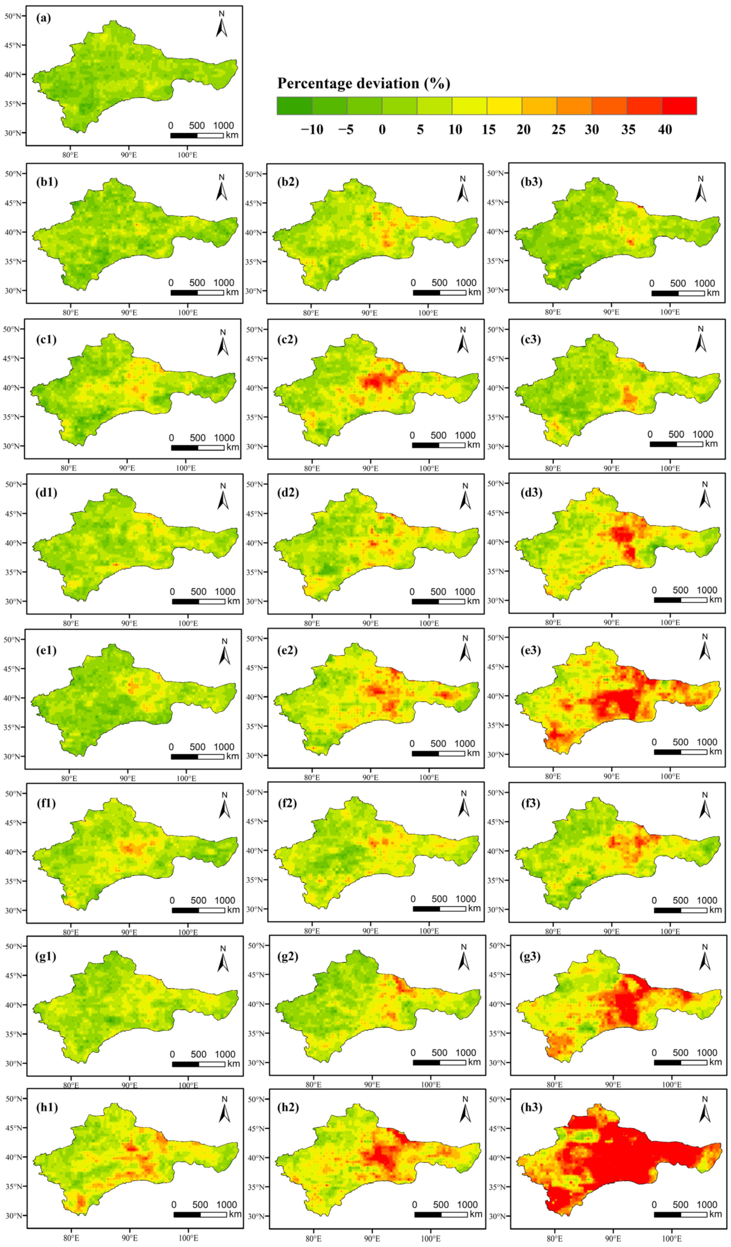
3.3. Exposure of Cropland

With or without consideration of the effect of CO₂, the results of drought exposure for cropland are as follows (Figure 10). During the baseline period, cropland exposure was approximately 92,000 km² per year, a reduction of approximately 21% compared to the condition without consideration of the effect of CO₂ (116,000 km² per year).

In terms of future projections, the cropland exposed to drought increases by 43% to 144% and by 42% to 164%, respectively, without and with the CO₂ effect, compared to the respective baseline period levels under all SSPs in the near-term; additionally, when the CO₂ effect is considered, cropland exposure is lower. Regardless of whether CO₂ is taken into account, cropland exposure under SSP1-2.6 is the lowest at 166,500 km² per year and 130,500 km² per year, respectively, an increase of two percentage points from the baseline period for the differences between cropland exposure without and with consideration of the CO₂ effect. Cropland exposure is the highest under SSP5-8.5, at 284,000 km² per year and 243,400 km² per year, respectively. When considering the difference in cropland exposure due to the inclusion or non-inclusion of the CO₂ effect, the largest difference of approximately 26% occurs under SSP3-7.0, while the smallest difference of only approximately 14% appears under SSP5-8.5. In addition, the GCM uncertainty is greatest under SSP1-2.6, at 243,000 km² per year (Figure 10a).

In the mid-term (Figure 10b), cropland exposure without the CO₂ effect is still greater than that without the CO₂ effect in all scenarios. Without considering the CO₂ effect, the maximum and minimum cropland exposure under SSP5-8.5 and SSP4-6.0 is 305,000 km² per year and 191,000 km² per year, respectively. Compared with the baseline period, only the increase rates under SSP3-7.0 and SSP4.60 are less than 100%, and the cropland exposure in the other scenarios is more than twice that of the baseline period. Taking the CO₂ effect into account, cropland exposure in all future scenarios increases over the baseline period, with increases ranging from 36% (SSP4-6.0) to 132% (SSP5-8.5). Cropland exposure reaches approximately 214,000 km² per year under SSP5-8.5, which is 2.3 times that of the baseline period. For the differences between cropland exposure with and without consideration of the effect of CO₂, the difference is the smallest under SSP1-1.9, which is approximately 16.7%, and the largest under SSP4-6.0, which can reach approximately 35.4%. The largest range of GCM uncertainty is under SSP1-2.6, with 232,000 km² per year and 272,000 km² per year, respectively, regardless of whether the CO₂ effect is considered.

In the long-term (Figure 10c), both with and without CO₂ consideration, cropland exposure to drought increases under all scenarios. However, the relatively lighter exposure of farmland when considering the CO₂ effect remains. When ignoring the CO₂ effect, the exposure of cropland under SSP1-2.6 is the lowest and increases by 81% compared with that of the baseline period. The rate of increase in cropland exposure in other scenarios exceeds 100% that of the baseline level. The exposure of cropland to drought under SSP5-8.5 reaches approximately 384,000 km² per year, 3.3 times that of the baseline period, and the rate of increase in exposure under SSP4-3.4 is the largest (approximately 475%), with an acreage of approximately 669,000 km² per year. When the CO₂ effect is considered, compared with the baseline period, cropland exposure increases by 69% to 164% in the long-term. The highest drought exposure on cropland occurs under SSP4-3.4, reaching approximately 524,000 km² per year. Unlike the case that does not consider the CO₂ effect, where the lowest exposure occurs under SSP1-2.6, the lowest exposure is approximately 156,000 km² per year under SSP3-7.0. In terms of the differences between the two sets of cropland exposure to drought, the difference between SSP1-1.9 and SSP1-2.6 is the smallest, and both are less than 50,000 km² per year. Then, the exposure difference between SSP2-4.5 and SSP4.6.0 is approximately 100,000 km² per year, while the largest exposure difference of 145,000 km² per year is under SSP4-3.4. It is worth mentioning that the main reason for the largest cropland exposure under SSP4-3.4 is the expansion of cropland acreage. According to the design of this scenario, the increase in carbon price leads to a significant increase in the total cropland area, with a rate of increase of 80% from 2010 to 2100 [47]. Meanwhile, the acreage of cropland in the study area is relatively small under other scenarios, and the change in cropland exposure is due to the change in the drought itself in this condition.

4. Conclusions and Discussion

A clear and quantitative understanding of the evolution of drought characteristics and the change in cropland exposure in the future is of great significance to water resource management, as well as social and economic development in the arid region of China. In this paper, seven GCMs, combined with dynamic land-use changes, are applied to study the future drought characteristics and changes in cropland exposure in the arid region of China. Furthermore, the projected impact of CO₂ concentrations on drought has been removed, providing a more comprehensive assessment of long-term water management. The main conclusions are as follows:

(1)

In 1961–2014, the SPEI shows an increasing trend (becoming wet), but the rate of SPEI increase is faster when considering the effect of CO₂ than without CO₂ (0.12/10a vs. 0.02/10a). The difference in drought intensity (approximately −1.45) is not obvious regardless of whether the CO₂ effect is considered in 1995–2014. Drought frequency decreases by 0.9 times/10a compared with the scenario in which CO₂ is ignored. The differences in drought duration and acreage caused by the CO₂ effect are approximately 1 month and 29%, respectively. The cropland exposure is approximately 92,000 km²/year when the CO₂ effect is considered, which is approximately 21% less than that without CO₂.

(2)

In the near-term, drought intensity is slightly more severe than in the baseline period, but weaker than that without the CO₂, and the maximum drought intensity difference is under SSP5-8.5 (11.4%). The decrease in drought frequency without the CO₂ effect is more obvious than that with CO₂, especially under SSP5-8.5. The difference between the arid acreage with and without CO₂ is the smallest under SSP4-6.0, while the largest difference occurs under SSP4-3.4. Cropland exposure without the CO₂ effect is still greater than that without the CO₂ effect in all scenarios (16.7–35.4%).

(3)

During the mid-term, drought intensity is further enhanced. Ignoring the CO₂ effect, drought frequency decreases compared with the baseline period, but increases with the CO₂ effect. Drought durations with the CO₂ effect are shorter than those without CO₂, with differences ranging from 3.2 months (SSP4-3.4) to 9.8 months (SSP5-8.5). Drought acreage is 1.5 times (SSP4-6.0) to 2.5 times (SSP1-1.9) that of the baseline period and 18.2–40.2% less than that without the CO₂ effect. Cropland exposure without CO₂ effect is still larger than that with the CO₂ effect considered (the differences range from 16.7% to 35.4%).

(4)

Regarding the long-term, the differences in drought intensity with and without the CO₂ effect are the largest in SSP5-8.5 (31.1%). Drought frequency shows a decreasing trend, and the effect of CO₂ on drought frequency increases with increasing emission concentrations. Drought acreage increases regardless of the CO₂ effect, and the maximum drought acreage considering the CO₂ effect is far smaller than that ignoring the CO₂ effect. Cropland exposure to drought increases in all scenarios, and from the perspective of the difference in cropland drought exposure with and without the CO₂ effect, the largest difference is 145,000 km²/year under SSP4-3.4.

The accurate estimation of PET is very important for drought assessment. A previous study proved that PET in the arid region of China is overestimated, by using the traditional PM formula according to surface meteorological observations and a variety of Moderate Resolution Imaging Spectroradiometer (MODIS) products [55]. For plant transpiration, as an important part of evapotranspiration, the change in CO₂ concentration will have an impact on of vegetation’s physiological characteristics. Previous studies have found that high CO₂ conditions can compensate for most of the impact of temperature rise on evapotranspiration through numerical experiments, which is consistent with our research view [30]. This PET overestimation using the traditional PM formula leads to deviations in drought assessment, and we can see that future drought risk will be more severe than that of the baseline period; however, the CO₂ effect will mitigate the risk slightly, according to our research. However, there are two main limitations in this paper. First, we followed the FAO’s hypotheses for the PM formula (Ⅰ: full evaporation is achieved under optimal soil moisture conditions and given climate conditions; Ⅱ: a crop height of 0.12 m and an albedo of 0.23 are used as a reference surface for evaporation) and modified only the parameter of surface resistance (establishing a relationship with CO₂ concentration). However, the type, quantity and distribution density of vegetation may affect PET in the real world. Second, the CO₂ concentration data used are estimated in only the latitudinal direction, and lack a detailed description in the longitudinal direction [56]; however, there is not much difference in the spatial distribution of CO₂ concentrations in the longitudinal direction for the arid region of China. Thus, the estimation of PET, as an important cause of drought, needs to take full account of various influencing factors and of the validation of existing methods in future research.

References

1. Dai, A.G. Drought under global warming: A review. Wiley Interdiscip. Rev. Clim. Chang. 2011, 2, 45–65. [Google Scholar] [CrossRef] [Green Version]
2. Chen, H.P.; Sun, J.Q. Changes in drought characteristics over China using the standardized precipitation evapotranspiration index. J. Clim. 2015, 28, 5430–5447. [Google Scholar] [CrossRef]
3. Dai, A.G.; Zhao, T.B.; Chen, J. Climate change and drought: A precipitation and evaporation perspective. Curr. Clim. Chang. Rep. 2018, 4, 301–312. [Google Scholar] [CrossRef]
4. Mishra, A.K.; Singh, V.P. A review of drought concepts. J. Hydrol. 2010, 391, 202–216. [Google Scholar] [CrossRef]
5. Duan, R.X.; Huang, G.H.; Zhou, X.; Li, Y.P.; Tian, C.Y. Ensemble drought exposure projection for multifactorial interactive effects of climate change and population dynamics: Application to the Pearl River Basin. Earth’s Future 2021, 9, 2215. [Google Scholar] [CrossRef]
6. Sheffield, J.; Wood, E.F.; Roderick, M.L. Little change in global drought over the past 60 years. Nature 2012, 491, 435–438. [Google Scholar] [CrossRef]
7. Wen, S.S.; Wang, A.Q.; Tao, H.; Malik, K.; Huang, J.L.; Zhai, J.Q.; Jing, C.; Rasul, G.; Su, B.D. Population exposed to drought under the 1.5 °C and 2.0 °C warming in the Indus River Basin. Atmos. Res. 2019, 218, 296–305. [Google Scholar] [CrossRef]
8. IPCC. Summary for Policymakers. In Climate Change 2022: Impacts, Adaptation, and Vulnerability. Contribution of Working Group II to the Sixth Assessment Report of the Intergovernmental Panel on Climate Change; Pörtner, H.-O., Roberts, D.C., Poloczanska, E.S., Mintenbeck, K., Tignor, M., Alegría, A., Craig, M., Langsdorf, S., Löschke, S., Möller, V., et al., Eds.; Cambridge University Press: Cambridge, UK, 2022. [Google Scholar]
9. Li, Q.Q.; Cao, Y.P.; Miao, S.L.; Huang, X.H. Spatiotemporal characteristics of drought and wet events and their impacts on agriculture in the Yellow River Basin. Land 2022, 11, 556. [Google Scholar] [CrossRef]
10. Dai, A.G. Increasing drought under global warming in observations and models. Nat. Clim. Chang. 2013, 3, 52–58. [Google Scholar] [CrossRef]
11. Trenberth, K.E.; Dai, A.G.; Van Der Schrier, G.; Jones, P.D.; Barichivich, J.; Briffa, K.R.; Sheffield, J. Global warming and changes in drought. Nat. Clim. Chang. 2014, 4, 17–22. [Google Scholar] [CrossRef]
12. Dai, A.G.; Zhao, T.B. Uncertainties in historical changes and future projections of drought. Part I: Estimates of historical drought changes. Clim. Chang. 2017, 144, 519–533. [Google Scholar] [CrossRef]
13. Su, B.D.; Huang, J.L.; Fischer, T.; Wang, Y.J.; Kundzewicz, Z.W.; Zhai, J.Q.; Sun, H.M.; Wang, A.Q.; Zeng, X.F.; Wang, G.J.; et al. Drought losses in China might double between the 1.5 ℃ and 2.0 ℃ warming. Proc. Natl. Acad. Sci. USA 2018, 115, 10600–10605. [Google Scholar] [CrossRef] [PubMed] [Green Version]
14. IPCC. Summary for Policymakers. In Climate Change 2021: The Physical Science Basis. Contribution of Working Group I to the Sixth Assessment Report of the Intergovernmental Panel on Climate Change; Masson-Delmotte, V.P., Zhai, A., Pirani, S.L., Connors, C., Péan, S., Berger, N., Caud, Y., Chen, L., Goldfarb, M.I., Gomis, M., et al., Eds.; Cambridge University Press: Cambridge, UK, 2021. [Google Scholar]
15. Sheffield, J.; Andreadis, K.M.; Wood, E.F.; Lettenmaier, D.P. Global and continental drought in the second half of the twentieth century: Severity–area–duration analysis and temporal variability of large-scale events. J. Clim. 2009, 22, 1962–1981. [Google Scholar] [CrossRef]
16. Su, B.D.; Huang, J.L.; Mondal, S.K.; Zhai, J.Q.; Wang, Y.J.; Wen, S.S.; Gao, M.N.; Lv, Y.R.; Jiang, S.; Jiang, T.; et al. Insight from CMIP6 SSP-RCP scenarios for future drought characteristics in China. Atmos. Res. 2021, 250, 105375. [Google Scholar] [CrossRef]
17. Zhai, J.Q.; Huang, J.L.; Su, B.D.; Cao, L.G.; Wang, Y.J.; Jiang, T.; Fischer, T. Intensity–area–duration analysis of droughts in China 1960–2013. Clim. Dyn. 2017, 48, 151–168. [Google Scholar] [CrossRef]
18. Zhou, J.; Wang, Y.J.; Su, B.D.; Wang, A.Q.; Tao, H.; Zhai, J.Q.; Kundzewicz, Z.W.; Jiang, T. Choice of potential evapotranspiration formulas influences drought assessment: A case study in China. Atmos. Res. 2020, 242, 104979. [Google Scholar] [CrossRef]
19. Shangguan, W.; Zhang, R.Q.; Li, L.; Zhang, S.L.; Zhang, Y.; Huang, F.N.; Li, J.D.; Liu, W. Assessment of agricultural drought based on reanalysis soil moisture in Southern China. Land 2022, 11, 502. [Google Scholar] [CrossRef]
20. Scheff, J.; Mankin, J.S.; Coats, S.; Liu, H. CO2-plant effects do not account for the gap between dryness indices and projected dryness impacts in CMIP6 or CMIP5. Environ. Res. Lett. 2021, 16, 034018. [Google Scholar] [CrossRef]
21. Milly, P.C.D.; Dunne, K.A. Potential evapotranspiration and continental drying. Nat. Clim. Chang. 2016, 6, 946–949. [Google Scholar] [CrossRef]
22. Zhou, J.; Jiang, S.; Su, B.D.; Huang, J.L.; Wang, Y.J.; Zhan, M.J.; Jing, C.; Jiang, T. Why the effect of CO2 on potential evapotranspiration estimation should be considered in future climate. Water 2022, 14, 986. [Google Scholar] [CrossRef]
23. Yuan, S.S.; Quiring, S.M. Drought in the US Great Plains (1980–2012): A sensitivity study using different methods for estimating potential evapotranspiration in the Palmer Drought Severity Index. J. Geophys. Res. Atmos. 2014, 119, 10996–11010. [Google Scholar] [CrossRef]
24. Dewes, C.F.; Rangwala, I.; Barsugli, J.J.; Hobbins, M.T.; Kumar, S. Drought risk assessment under climate change is sensitive to methodological choices for the estimation of evaporative demand. PLoS ONE 2017, 12, e0174045. [Google Scholar] [CrossRef] [PubMed] [Green Version]
25. Allen, R.G.; Pereira, L.S.; Raes, D.; Smith, M. Crop Evapotranspiration: Guidelines for Computing Crop Water Requirements; FAO Irrigation and Drainage Paper 56; FAO: Rome, Italy, 1998; Available online: http://www.fao.org/docrep/X0490E/X0490E00.htm (accessed on 4 May 2022).
26. Shi, L.J.; Feng, P.Y.; Wang, B.; Liu, D.L.; Cleverly, J.; Fang, Q.X.; Yu, Q. Projecting potential evapotranspiration change and quantifying its uncertainty under future climate scenarios: A case study in southeastern Australia. J. Hydrol. 2020, 584, 124756. [Google Scholar] [CrossRef]
27. Xiang, K.Y.; Li, Y.; Horton, R.; Feng, H. Similarity and difference of potential evapotranspiration and reference crop evapotranspiration-A review. Agric. Water Manag. 2020, 232, 106043. [Google Scholar] [CrossRef]
28. Yang, Y.T.; Roderick, M.L.; Zhang, S.L.; McVicar, T.R.; Donohue, R.J. Hydrologic implications of vegetation re-sponse to elevated CO2 in climate projections. Nat. Clim. Chang. 2019, 9, 44–49. [Google Scholar] [CrossRef]
29. Roderick, M.L.; Greve, P.; Farquhar, G.D. On the assessment of aridity with changes in atmospheric CO2. Water Resour. Res. 2015, 51, 5450–5463. [Google Scholar] [CrossRef] [Green Version]
30. Swann, A.L.S.; Hoffman, F.M.; Koven, C.D.; Randerson, J.T. Plant responses to increasing CO2 reduce estimates of climate impacts on drought severity. Proc. Natl. Acad. Sci. USA 2016, 113, 10019–10024. [Google Scholar] [CrossRef] [Green Version]
31. Mishra, V.; Thirumalai, K.; Singh, D.; Aadhar, S. Future exacerbation of hot and dry summer monsoon extremes in India. NPJ Clim. Atmos. Sci. 2020, 3, 1–9. [Google Scholar] [CrossRef]
32. Chai, R.F.; Mao, J.F.; Chen, H.S.; Wang, Y.P.; Shi, X.Y.; Jin, M.Z.; Zhao, T.B.; Hoffman, F.M.; Ricciuto, D.M.; Wullschleger, S.D. Human-caused long-term changes in global aridity. NPJ Clim. Atmos. Sci. 2021, 4, 65. [Google Scholar] [CrossRef]
33. Field, C.B.; Jackson, R.B.; Mooney, H.A. Stomatal responses to increased CO2: Implications from the plant to the global scale. Plant Cell Environ. 1995, 18, 1214–1225. [Google Scholar] [CrossRef]
34. Novick, K.; Ficklin, D.; Stoy, P.; Williams, C.A.; Bohrer, G.; Oishi, A.C.; Papuga, S.A.; Blanken, P.D.; Noormets, A.; Sulman, B.N.; et al. The increasing importance of atmospheric demand for ecosystem water and carbon fluxes. Nat. Clim. Chang. 2016, 6, 1023–1027. [Google Scholar] [CrossRef] [Green Version]
35. Lian, X.; Piao, S.L.; Chen, A.P.; Huntingford, C.; Fu, B.J.; Li, L.Z.X.; Huang, J.P.; Sheffield, J.; Berg, A.M.; Keenan, T.F.; et al. Multifaceted characteristics of dryland aridity changes in a warming world. Nat. Rev. Earth Environ. 2021, 2, 232–250. [Google Scholar] [CrossRef]
36. Zhai, J.Q.; Mondal, S.K.; Fischer, T.; Wang, Y.J.; Su, B.D.; Huang, J.L.; Tao, H.; Wang, G.J.; Ullah, W.; Uddin, M.J. Future drought characteristics through a multi-model ensemble from CMIP6 over South Asia. Atmos. Res. 2020, 246, 105111. [Google Scholar] [CrossRef]
37. Mondal, S.K.; Huang, J.L.; Wang, Y.J.; Su, B.D.; Zhai, J.Q.; Tao, H.; Wang, G.J.; Fischer, T.; Wen, S.S.; Jiang, T. Doubling of the population exposed to drought over South Asia: CMIP6 multi-model-based analysis. Sci. Total Environ. 2021, 771, 145186. [Google Scholar] [CrossRef] [PubMed]
38. Yang, P.; Xia, J.; Zhang, Y.Y.; Zhan, C.S.; Cai, W.; Zhang, S.Q.; Wang, W.Y. Quantitative study on characteristics of hydrological drought in arid area of northwest China under changing environment. J. Hydrol. 2021, 597, 126343. [Google Scholar] [CrossRef]
39. Chen, Y.N.; Li, Z.; Li, W.H.; Deng, H.J.; Shen, Y.J. Water and ecological security: Dealing with hydroclimatic challenges at the heart of China’s Silk Road. Environ. Earth Sci. 2016, 75, 1–10. [Google Scholar] [CrossRef]
40. Shi, Y.F.; Shen, Y.P.; Hu, R.J. Preliminary study on signal, impact and foreground of climatic shift from warm-dry to warm-humid in Northwest China. J. Glaciol. Geocryol. 2002, 24, 219–226. [Google Scholar]
41. Wang, Y.J.; Qin, D.H. Influence of climate change and human activity on water resources in arid region of Northwest China: An overview. Adv. Clim. Chang. Res. 2017, 8, 268–278. [Google Scholar] [CrossRef]
42. Yuan, Q.Z.; Wu, S.H.; Dai, E.F.; Zhao, D.S.; Zhang, X.R.; Ren, P. Spatio-temporal variation of the wet-dry conditions from 1961 to 2015 in China. Sci. China Earth Sci. 2017, 60, 2041–2050. [Google Scholar] [CrossRef]
43. Yang, P.; Xia, J.; Zhan, C.S.; Zhang, Y.Y.; Hu, S. Discrete wavelet transform-based investigation into the variability of standardized precipitation index in Northwest China during 1960–2014. Theor. Appl. Climatol. 2018, 132, 167–180. [Google Scholar] [CrossRef]
44. Huang, J.L.; Zhai, J.Q.; Jiang, T.; Wang, Y.J.; Li, X.C.; Wang, R.; Xiong, M.; Su, B.D.; Fischer, T. Analysis of future drought characteristics in China using the regional climate model CCLM. Clim. Dyn. 2018, 50, 507–525. [Google Scholar] [CrossRef]
45. Li, S.Y.; Miao, L.J.; Jiang, Z.H.; Wang, G.J.; Gnyawali, K.R.; Zhang, J.; Zhang, H.; Fang, K.; He, Y.; Li, C. Projected drought conditions in Northwest China with CMIP6 models under combined SSPs and RCPs for 2015–2099. Adv. Clim. Chang. Res. 2020, 11, 210–217. [Google Scholar] [CrossRef]
46. Su, B.D.; Huang, J.L.; Gemmer, M.; Jian, D.N.; Tao, H.; Jiang, T.; Zhao, C.Y. Statistical downscaling of CMIP5 multi-model ensemble for projected changes of climate in the Indus River Basin. Atmos. Res. 2016, 178, 138–149. [Google Scholar] [CrossRef]
47. Meinshausen, M.; Vogel, E.; Nauels, A.; Lorbacher, K.; Meinshausen, N.; Etheridge, D.M.; Fraser, P.J.; Montzka, S.A.; Rayner, P.J.; Trudinger, C.M.; et al. Historical greenhouse gas concentrations for climate modelling (CMIP6). Geosci. Model Dev. 2017, 10, 2057–2116. [Google Scholar] [CrossRef] [Green Version]
48. Meinshausen, M.; Nicholls, Z.R.J.; Lewis, J.; Gidden, M.J.; Vogel, E.; Freund, M.; Beyerle, U.; Gessner, C.; Nauels, A.; Bauer, N.; et al. The shared socio-economic pathway (SSP) greenhouse gas concentrations and their extensions to 2500. Geosci. Model Dev. 2020, 13, 3571–3605. [Google Scholar] [CrossRef]
49. Hurtt, G.C.; Chini, L.; Sahajpal, R.; Frolking, S.; Bodirsky, B.L.; Calvin, K.; Doelman, J.C.; Fisk, J.; Fujimori, S.; Goldewijk, K.K.; et al. Harmonization of global land use change and management for the period 850–2100 (LUH2) for CMIP6. Geosci. Model Dev. 2020, 13, 5425–5464. [Google Scholar] [CrossRef]
50. Popp, A.; Calvin, K.; Fujimori, S.; Havlik, P.; Humpenöder, F.; Stehfest, E.; Bodirsky, B.L.; Dietrich, J.P.; Doelmann, J.C.; Gusti, M.; et al. Land-use futures in the shared socio-economic pathways. Global Environ. Chang. 2017, 42, 331–345. [Google Scholar] [CrossRef] [Green Version]
51. Yang, Y.T.; Zhang, S.L.; Roderick, M.; McVicar, T.R.; Yang, D.W.; Liu, W.B.; Li, X.Y. Comparing Palmer Drought Severity Index drought assessments using the traditional offline approach with direct climate model outputs. Hydrol. Earth Syst. Sci. 2020, 24, 2921–2930. [Google Scholar] [CrossRef]
52. Vicente-Serrano, S.M.; Beguería, S.; López-Moreno, J.I. A multiscalar drought index sensitive to global warming: The standardized precipitation evapotranspiration index. J. Clim. 2010, 23, 1696–1718. [Google Scholar] [CrossRef] [Green Version]
53. Palmer, W.C. Meteorological Drought, Research Paper No. 45; U.S. Department of Commerce: Washington, DC, USA, 1965.
54. Cook, B.I.; Smerdon, J.E.; Seager, R.; Coats, S. Global warming and 21st century drying. Clim. Dyn. 2014, 43, 2607–2627. [Google Scholar] [CrossRef] [Green Version]
55. Hua, D.; Hao, X.M.; Zhang, Y.; Qin, J.X. Uncertainty assessment of potential evapotranspiration in arid areas, as estimated by the Penman-Monteith method. J. Arid. Land 2020, 12, 166–180. [Google Scholar] [CrossRef] [Green Version]
56. Cheng, W.; Dan, L.; Deng, X.Z.; Feng, J.M.; Wang, Y.L.; Peng, J.; Tian, J.; Qi, W.; Liu, Z.; Zheng, X.Q.; et al. Global monthly gridded atmospheric carbon dioxide concentrations under the historical and future scenarios. Sci. Data 2022, 9, 1–13. [Google Scholar] [CrossRef]
Figure 1. Location of the arid region in China.
Land 11 00881 g001
Figure 2. Comparison of the annual SPEI with and without the CO2 effect in 1961–2014 (a) and 2015–2100 (bh) under the SSPs.
Land 11 00881 g002
Figure 3. Spatial pattern of the SPEI-based drought trends in 1961–2014 (a1,a2) and 2015–2100 (b1h2) over the arid region of China without (left column) and with (right column) consideration of the CO2 effect. Note: Black crosses represent the grids with trends of SPEI agreement over 85%.
Land 11 00881 g003
Figure 4. Comparison of drought intensity with and without the CO2 effect in the near-term (a), mid-term (b) and long-term (c).
Land 11 00881 g004
Figure 5. The deviation in the spatial distribution of drought intensity without consideration of the effect of CO2 and considering the effect of CO2 for the baseline period (a), near-term (b1,c1,d1,e1,f1,g1,h1), mid-term (b2,c2,d2,e2,f2,g2,h2) and long-term (b3,c3,d3,e3,f3,g3,h3).
Land 11 00881 g005
Figure 6. Comparison of drought frequency with and without the CO2 effect in the near-term (a), mid-term (b) and long-term (c).
Land 11 00881 g006
Figure 7. The spatial distribution of drought frequency differences without and with consideration of the effect of CO2 for the baseline period (a), near-term (b1,c1,d1,e1,f1,g1,h1), mid-term (b2,c2,d2,e2,f2,g2,h2) and long-term (b3,c3,d3,e3,f3,g3,h3).
Land 11 00881 g007
Figure 8. Comparison of drought duration with and without the CO2 effect in the near-term (a), mid-term (b) and long-term (c).
Land 11 00881 g008
Figure 9. Comparison of drought acreage with and without the CO2 effect in the near-term (a), mid-term (b) and long-term (c).
Land 11 00881 g009
Figure 10. Comparison of cropland exposure to drought with and without the CO2 effect in the near-term (a), mid-term (b) and long-term (c).
Land 11 00881 g010