The Time-Varying Effect of Interest Rates on Housing Prices

Abstract

This study analyzes the time-varying effect of interest rates on housing prices. As housing prices are too high for most consumers to afford with income alone, they use bank loans. Consequently, when interest rates fall, the demand for housing increases, causing prices to rise. This effect of interest rates was common in countries that implemented low-interest rates in response to the COVID-19 pandemic. Using Korean data from March 1991 to March 2022, this study examined the impact of interest rate shocks on housing prices by employing a time-varying parameter vector autoregressive model. According to the analysis, in Korea, while the impact of the interest rate shocks on housing prices was not significant before the global financial crisis, it increased dramatically afterward. Particularly, the impact of interest rate shocks was strongest relative to the past during the period of the increase in house prices from 2020 to 2021. The rise in the effects of interest rate shocks on housing prices is attributed to the increased dependence on loans for housing purchases. The results suggest that given the recent substantial increments in interest rates due to inflation, an interest rate shock would likely cause a global housing market recession.

1. Introduction

As most housing consumers cannot afford housing prices, transactions cannot occur at the actual demand level. However, improving their ability to pay for housing by increasing their income or lowering their loan interest rates may lead to increased housing consumption. It is difficult for consumers to increase their income in a short period to the extent that the housing consumption is affected. However, by lowering the interest rates, consumers can easily procure large sums of money that would be difficult to obtain from their income alone, thereby significantly improving their ability to pay for housing in a short period. As the housing market supply is inelastic in the short term, if market demand increases due to consumers’ improved ability to pay for housing, housing prices will rise [1].

Recognizing that interest rates make a sizeable contribution to the housing demand, this study seeks to analyze the effect of interest rates on housing prices from a long-term perspective. Prior studies generally assume that the relationship between the interest rates and housing prices is time-invariant, and thus apply the constant vector autoregressive (VAR) model for the analysis and conclude that interest rates and housing prices have a negative relationship. However, these research findings are limited because they assume that interest rate shocks have a constant effect on housing prices even in different situations depending on the period, such as when interest rates are high or low and when the real economy is strong or weak. Borrowers’ dependence on loans varies with the interest rate levels. Therefore, while the government lowering the base rate when interest rates are high and raising it when interest rates are low are both the same policy in terms of lowering interest rates, the effects of these two events may differ because the cost of borrowing an identical amount varies with the interest rate level. Similarly, the interest rate shock when interest rates are raised may be asymmetrical to that when interest rates are lowered.

From 2020 to 2021, many have experienced a rapid climb in housing prices across Korea, and at this time, the causes of steep hikes in housing prices have been at the forefront of various debates for researchers and policymakers. According to Yoon [2], a possible reason for this might be the supply–demand imbalance due to dwindling supplies in housing. In the same vein, a recent investigation by the Bank of Korea (BOK) found that national market forces, such as the gaps between supply and demand, are obviously important determinants rather than other factors like the interest rate [3]. A broader perspective has also been argued that demand control policies including property ownership and acquisition tax increases and the increased regulatory measures on the LTV (loan-to-value ratio) caused a decrease in the supply of houses and thus a rise in housing prices [4]. Lee [5] highlights tightening regulatory measures to suppress demands such as designating either “regulated areas” or “overheated speculative zones” as the major causes of the housing price hike. Unlike previously aforementioned studies, Cho’s study [6] identified the relevance of the media’s report on the expectations of a rise in housing prices in determining housing prices. The proposed argument might increase the asking price in housing, but ultimately, in order for the housing price to be determined as the market price, it can be realized only by paying a high asking price. Park [7] argued that, to demonstrate this, an improvement in the solvency must be accompanied and the temporary improvement in the solvency depends on lowering the interest rate. The most critical limitation lies in the fact that most empirical studies conducted so far assume that the influence of interest rates on housing prices is constant. We thus believe that this study provides a novel approach to the experiment using the time-varying parameter (TVP-VAR) model whether the impact of the interest rates on housing prices varies over time. The TVP-VAR model was mainly used in research on the monetary policies (e.g., [8]). This study seeks to analyze the relationship between interest rates and housing prices from the perspective that the impact of interest rates varies over time. To this end, we establish the following empirical analysis strategy to identify the time-varying effects of interest rates and housing prices. First, an impulse response function based on the constant VAR model, which has been used in most prior empirical studies on interest rates and housing prices, is obtained. Second, we apply a local projection method [9] while relaxing the assumption of the first analysis, that the mean and variance are constant and assuming that the mean and variance for a certain period may differ, and use this to analyze the influence of interest rate shocks on housing prices during the rising and falling of interest rates. Third, we analyze the influence of interest rate shocks on housing prices based on the time-varying parameter VAR model [8], while further relaxing the assumption of the second analysis and assuming that the relationship between interest rates and housing prices at each point in time can differ. Through this analysis strategy, we expect to clearly identify the impact of interest rates on the housing market by the interest rate period in Korea and the long-term structural break between interest rates and the housing market.

The remainder of this paper is structured as follows: Section 2 reviews the prior studies related to the subject of this study and discusses how this study is different from them. Section 3 introduces the analysis model design and data used in this study. Section 4 examines the analysis results of the constant VAR impulse response function (IRF), conditional local projection, and time-varying parameter VAR IRF. Section 5 summarizes the content of this study and presents policy implications, limitations, and future research directions.

2. Literature Review

Among the major empirical studies on interest rates and housing prices in Korea, many have focused on the influence of interest rate changes on housing prices; however, most are based on time-invariant effects, while some have attempted conditional analyses.

First, numerous studies on interest rates and housing prices report that interest rates and housing prices have a negative relationship; however, researchers have confirmed that the statistical significance varies with the conditions of the analysis sample [7,10,11,12,13,14,15]. These studies were generally conducted under the assumption that the mean and variance were constant at all time points.

Studies that conducted an unconditional analysis of the sample have demonstrated changes in interest rate policies, such as monetary authorities actively managing accommodative monetary measures during rapid fluctuations in the real economy due to events such as a foreign exchange crisis, global financial crisis, the COVID-19 pandemic, and so on. However, many studies have also performed analyses without considering these periods, and they typically tend not to identify the impact of interest rate shocks on housing prices [10,13].

Regarding conditional analysis studies that divided the analysis sample into before and after an economic crisis, when the analysis sample was divided into before and after the foreign exchange crisis, researchers found that the impact of interest rate shocks tended to decrease after the financial crisis [11]. Researchers have also analyzed samples before and after the global financial crisis and found that the impact of interest rate shocks on housing prices differs before and after [12,15]. However, these studies have limitations because they assume that the impact of interest rate shocks during rising and falling interest rates is symmetrical.

Regarding conditional analysis studies that divided the time periods of rising and falling interest rates, a study combined the analysis samples in four combinations according to rising and falling interest rates and rising and falling prices; the impact of interest rate shocks on housing prices differed under each given condition [14]. Additionally, a study that divided the analysis sample into before and after a monetary policy transition found that the contribution of interest rates to the rise in housing prices greatly increased with the transition to low-interest rates [7]. However, these studies also have limitations, as they assume that the impact of interest rate shocks is unvarying even at the absolute level of interest rates.

Taken together, researchers have found that interest rates and housing prices have a negative relationship, but their approaches have comprised the unconditional analysis of the sample under the assumption that the regime is constant throughout the analysis period and conditional analysis under the assumptions that an economic crisis and interest rate changes are a signal of a regime switch. These studies have limitations, as they view the timing of rising and falling interest rates as symmetrical, or shocks that occur at each interest rate level as unvarying.

Thus, we confirm that most previous studies assume the impact of interest rates to be time-invariant or time-invariant under a certain regime. Unlike prior research, this study assumes that the impact of interest rates between the periods of rising and falling interest rates differs and that the impact of interest rates can differ at each point in time. For the analysis, we use the local projection method and time-varying parameter VAR (TVP-VAR) model to improve on the limitations of the existing studies.

3. Research Design

The purpose of this study is to analyze the time-varying effect of interest rates on housing prices and the varying impacts of interest rates during periods of rising and falling interest rates. To clearly observe the time-varying effect of interest rates, we estimate the time-invariant IRF, conditional IRF, and time-varying IRF in stages.

The conditional IRF uses the local projection method that estimates the IRF between the explanatory and the dependent variable. The IRF can be estimated by setting conditions for a given economic situation, such as interest rates or the market situation. The IRF is generally estimated using the VAR model; however, if the data generation process does not follow the VAR process, then a suitable IRF cannot be derived due to setting errors [9].

The local projection method adds one future time point at a time to construct h regression equations and interprets the coefficient value of the regression equations as the impulse response value. The IRF estimated with the local projection method is identical to that estimated with VAR when the conditions match.

Equation (1) shows the relationship between the interest rate at time t and the housing price change rate at time t + h. In this study, the time lag is set from 1 month to 24 months in the future.

$${\mathsf{\Delta }\mathrm{P}}_{\mathrm{t}+\mathrm{h}}={\mathsf{\beta }}_0+{\mathsf{\beta }}_{\mathrm{h}}{\mathrm{r}}_{\mathrm{t}}+{\mathrm{X}}^{\prime }\mathsf{\Gamma }+{\mathsf{\epsilon }}_{\mathrm{t}+\mathrm{h}}$$

(1)

$$\mathrm{h}=1,2,3, \dots , 24.$$

As the objective of monetary policy is to converge the inflation rate to a certain level in the medium term, monetary policy involves a process of repeatedly raising and lowering the base rate for a certain period. The general VAR model assumes that interest rate shocks during periods of rising and falling interest rates are symmetrical. This study divides the analysis sample into the period of rising interest rates and that of falling interest rates based on the base rate to analyze the IRF according to Equation (1) and identify the asymmetry of housing price responses to interest rate shocks.

Empirical studies related to interest rates and housing prices confirmed that the impact of interest rates weakened after the foreign exchange crisis and strengthened after the global financial crisis [11,12,15]. Considering that the base rate system was introduced after the foreign exchange crisis, the analysis sample is divided into before and after the global financial crisis to analyze the asymmetry of interest rate shocks.

Next, we use the TVP-VAR model to investigate the time-varying effect of interest rates. The TVP-VAR model can confirm the time-varying effect of interest rate shocks by estimating the IRF at a specific point in time based on the Markov chain Monte Carlo (MCMC) simulation.

As the VAR model estimates the IRF that applies to all periods, even if the impact of interest rates grows at a specific time point, it cannot estimate the impact at each time point. The TVP-VAR model can estimate the IRF at a specific time point, so it can identify the structural break characteristics and time-varying impact of interest rates. The TVP-VAR model analyzes the time-varying impact based on Gibbs sampling, an MCMC simulation method, and the Bayesian statistical inference technique.

Specifically, the model used in this study is based on the following TVP-VAR model [8]. First, to understand the model, we introduce the following n-variable VAR model.

$${\mathrm{Y}}_{\mathrm{t}} = {\mathrm{c}}_{\mathrm{t}} + {{\displaystyle \sum }}_{\mathrm{k} = 1}^{\mathrm{K}}{\mathrm{B}}_{\mathrm{k},\mathrm{t}}{\mathrm{Y}}_{\mathrm{t}-\mathrm{k}}+{\mathrm{u}}_{\mathrm{t}},$$

(2)

where ${\mathrm{Y}}_{\mathrm{t}}$ is a matrix of ($\mathrm{n}\times 1$) the endogenous variables, $\mathrm{k}$ is the time lag, ${\mathrm{B}}_{\mathrm{t}}$ is the ($\mathrm{n}\times \mathrm{n}$) time-varying coefficient matrix, and ${\mathrm{u}}_{\mathrm{t}}$ is the heterogeneous unobserved shock of the variance–covariance matrix ${\mathsf{\Omega }}_{\mathrm{t}}$. It is assumed that the variance–covariance matrix can be written as follows:

$$\mathrm{Var}\left({\mathrm{u}}_{\mathrm{t}}\right) = {\mathsf{\Omega }}_{\mathrm{t}} = {\mathrm{A}}_{\mathrm{t}}{}^{-1}{\mathsf{\Sigma }}_{\mathrm{t}}{{\mathsf{\Sigma }}_{\mathrm{t}}}^{\prime }{\left({\mathrm{A}}_{\mathrm{t}}{}^{-1}\right)}^{\prime }.$$

(3)

${\mathrm{A}}_{\mathrm{t}}$ in Equation (3) is composed of the following lower triangular matrix:

$${\mathrm{A}}_{\mathrm{t}} = \left[\begin{array}{cccc}1& 0& \cdots & 0\\ {\mathsf{\alpha }}_{2 1, \mathrm{t}}& 1& \ddots & ⋮\\ ⋮& \ddots & \ddots & 0\\ {\mathsf{\alpha }}_{\mathrm{n} 1, \mathrm{t}}& \cdots & {\mathsf{\alpha }}_{\mathrm{n} \mathrm{n}-1, \mathrm{t}}& 1\end{array}\right].$$

(4)

${\mathsf{\Sigma }}_{\mathrm{t}}$ in Equation (3) is assumed to be composed of the diagonal matrix of variance.

$${\mathsf{\Sigma }}_{\mathrm{t}} = \left[\begin{array}{cccc}{\mathsf{\sigma }}_{1, \mathrm{t}}& 0& \cdots & 0\\ 0& {\mathsf{\sigma }}_{2, \mathrm{t}}& \ddots & ⋮\\ ⋮& \ddots & \ddots & 0\\ 0& \cdots & 0& {\mathsf{\sigma }}_{\mathrm{n}, \mathrm{t}}\end{array}\right].$$

(5)

If ${\mathsf{\epsilon }}_{\mathrm{t}} = {\mathrm{I}}_{\mathrm{n}}$ is defined, then the residual of Equation (2) can be defined as ${\mathrm{u}}_{\mathrm{t}} = {\mathrm{A}}_{\mathrm{t}}{}^{-1}{\mathsf{\Sigma }}_{\mathrm{t}}{\mathsf{\epsilon }}_{\mathrm{t}}$, so Equation (2) can be expressed as Equation (6):

$${\mathrm{Y}}_{\mathrm{t}} = {\mathrm{c}}_{\mathrm{t}}+{{\displaystyle \sum }}_{\mathrm{k}=1}^{\mathrm{K}}{\mathrm{B}}_{\mathrm{k},\mathrm{t}}{\mathrm{Y}}_{\mathrm{t}-\mathrm{k}}+{\mathrm{A}}_{\mathrm{t}}{}^{-1}{\mathsf{\Sigma }}_{\mathrm{t}}{\mathsf{\epsilon }}_{\mathrm{t}}.$$

(6)

The most significant feature of the TVP-VAR model is that the coefficient value changes over time, so it assumes a stochastic process through a random walk process.

$${\mathrm{B}}_{\mathrm{t}} = {\mathrm{B}}_{\mathrm{t}-1} + {\mathsf{\kappa }\mathsf{\nu }}_{\mathrm{t}},$$

(7)

$${\mathsf{\alpha }}_{ \mathrm{t}}={\mathsf{\alpha }}_{\mathrm{t}-1}+{\mathsf{\kappa }\mathsf{\zeta }}_{\mathrm{t}},$$

(8)

$${\log \mathsf{\sigma }}_{\mathrm{t}}={\log \mathsf{\sigma }}_{ \mathrm{t}-1}+{\mathsf{\kappa }\mathsf{\eta }}_{\mathrm{t}}.$$

(9)

The residual component ${\mathsf{\epsilon }}_{\mathrm{t}}$ derived from Equations (2) and (3) is the identity matrix, and error ${\mathsf{\kappa }\mathrm{v}}_{\mathrm{t}}$ of the time-varying coefficient matrix ${\mathrm{B}}_{\mathrm{t}}$ as well as errors ${\mathsf{\kappa }\mathsf{\zeta }}_{\mathrm{t}}$ and ${\mathsf{\kappa }\mathsf{\eta }}_{\mathrm{t}}$ of the variance–covariance components ${\mathsf{\alpha }}_{\mathrm{t}}$ and ${\mathsf{\sigma }}_{\mathrm{t}}$ are all stochastic processes. To reduce the number of estimated parameters, it is modeled as a random walk process.

In a general linear VAR model, when $\mathsf{\kappa } = 0$, all the time variances are equal, whereas in TVP-VAR, $\mathsf{\kappa } = 1$, the error is defined by a stochastic process.

Through this, the TVP-VAR system assumes the following variance–covariance matrix with a jointly normal distribution composed of one identity matrix and three random error vectors.

$$\mathrm{V} = \mathrm{Var}(\left[\begin{array}{c}{\mathsf{\epsilon }}_{\mathrm{t}}\\ {\mathsf{\nu }}_{\mathrm{t}}\\ {\mathsf{\zeta }}_{\mathrm{t}}\\ {\mathsf{\eta }}_{\mathrm{t}}\end{array}\right]) = \left[\begin{array}{cccc}{\mathrm{I}}_{\mathrm{n}}& 0& 0& 0\\ 0& \mathrm{Q}& 0& 0\\ 0& 0& \mathrm{S}& 0\\ 0& 0& 0& \mathrm{W}\end{array}\right]\equiv \left[\begin{array}{cccc}{\mathrm{I}}_{\mathrm{n}}& 0& 0& 0\\ 0& {\mathsf{\Sigma }}_{\mathsf{\beta }}& 0& 0\\ 0& 0& {\mathsf{\Sigma }}_{\mathrm{a}}& 0\\ 0& 0& 0& {\mathsf{\Sigma }}_{\mathrm{h}}\end{array}\right].$$

(10)

The time-varying posterior distribution estimation method of TVP-VAR uses Gibbs sampling. Although the TVP-VAR model is used for estimating the time-varying effects of the shocks, the time-varying effects are not only difficult to decompose in a residual structure, but also not actually observed. This makes it difficult to mathematically organize the posterior density function and derive it as a standard distribution, making it impossible to infer the posterior distribution.

Bayesian inference treats these unobserved parameters as random variables. Particularly, when the analysis target is a high dimensional parameter space, the MCMC method is optimal for numerically maximizing the posterior distributions, and a representative simulation method is Gibbs sampling. In the linear regression equation, assuming that the regression coefficient vector is $\mathsf{\beta }$ and the variance of the residual term is ${\mathsf{\sigma }}^2$, if ${\mathsf{\sigma }}^2$ is known, then $\mathsf{\beta }$ can be extracted from $\mathsf{\beta }\mid \mathrm{Y}$ and ${\mathsf{\sigma }}^2$, and it can be proven that the posterior distribution is a multivariate normal distribution. Conversely, if $\mathsf{\beta }$ is known, then ${\mathsf{\sigma }}^2$ can be extracted from ${\mathsf{\sigma }}^2\mid \mathrm{Y}$ and $\mathsf{\beta }$, in which case the posterior distribution is an inverse gamma distribution [16]. For example, the Gibbs sampling technique extracts a sufficient number of samples by repeating $\mathsf{\beta }\mid \mathrm{Y}$, ${\mathsf{\sigma }}^2$, ${\mathsf{\sigma }}^2\mid \mathrm{Y}$, and $\mathsf{\beta }$, and the posterior mean and posterior variance–covariance of the parameter distribution can also be estimated from these extracted samples. The TVP-VAR model is an estimation method that estimates the posterior distribution of the parameters using Gibbs sampling.

The analysis algorithm is presented as follows:

First, this study applies Gibbs sampling, an MCMC simulation technique, and assumes the distribution of hyperparameters $\mathrm{Q}$, $\mathrm{S}$, and $\mathrm{W}$ of Equation (10) through inverse Wishart for inference. Gibbs sampling sequentially estimates the time-varying coefficient (${\mathrm{B}}^{\mathrm{T}}$), simultaneity (${\mathrm{A}}^{\mathrm{T}}$), volatility (${\mathsf{\Sigma }}^{\mathrm{T}}$), and hyperparameter ($\mathrm{V}$) according to the observed data and remaining parameters, and $\mathrm{p}()$ indicates the density function. The initial value is set to the ordinary least squares coefficient value estimated with VAR using the prior sample.

$${\mathrm{A}}^{\mathrm{T}},{\mathsf{\Sigma }}^{\mathrm{T}},{\mathrm{s}}^{\mathrm{T}},\mathrm{V}\mathrm{initial}\mathrm{setting}$$

(11)

Based on the first initial value, sampling is performed as follows:

$$\mathrm{p}\left({\mathrm{B}}^{\mathrm{T}}\mid {\mathrm{y}}^{\mathrm{T}}, {\mathrm{A}}^{\mathrm{T}}, {\mathsf{\Sigma }}^{\mathrm{T}}, \mathrm{V}\right)\to {\mathrm{B}}^{\mathrm{T}},$$

(12)

$$\mathrm{p}\left({\mathrm{A}}^{\mathrm{T}}\mid {\mathrm{y}}^{\mathrm{T}}, {\mathrm{B}}^{\mathrm{T}}, {\mathsf{\Sigma }}^{\mathrm{T}}, \mathrm{V}\right)\to {\mathrm{A}}^{\mathrm{T}},$$

(13)

$$\mathrm{p}\left({\mathsf{\Sigma }}^{\mathrm{T}}\mid {\mathrm{y}}^{\mathrm{T}}, {\mathrm{A}}^{\mathrm{T}}, {\mathrm{B}}^{\mathrm{T}}, {\mathrm{s}}^{\mathrm{T}},\mathrm{V}\right)\to {\mathsf{\Sigma }}^{\mathrm{T}},$$

(14)

$$\mathrm{p}\left({\mathrm{s}}^{\mathrm{T}}\mid {\mathrm{y}}^{\mathrm{T}}, {\mathrm{A}}^{\mathrm{T}}, {\mathsf{\Sigma }}^{\mathrm{T}},\mathrm{V}\right)\to {\mathrm{s}}^{\mathrm{T}}.$$

(15)

In Equation (16), using the values extracted from Equations (12) to (15), $\mathrm{Q}$, $\mathrm{W}$, and $\mathrm{S}$ are extracted to extract $\mathrm{V}$, after which we return to Equation (11), re-extract the sample, and repeat this process 10,000 times.

$$\begin{gathered} \mathrm{p}\left(\mathrm{Q}, \mathrm{W}, \mathrm{S} \mid {\mathrm{y}}^{\mathrm{T}}, {\mathrm{B}}^{\mathrm{T}}, {\mathrm{A}}^{\mathrm{T}}, {\mathsf{\Sigma }}^{\mathrm{T}}\right)=\mathrm{p}\left(\mathrm{Q} \mid {\mathrm{y}}^{\mathrm{T}}, {\mathrm{B}}^{\mathrm{T}}, {\mathrm{A}}^{\mathrm{T}}, {\mathsf{\Sigma }}^{\mathrm{T}}\right)· \\ \mathrm{p}\left(\mathrm{W} \mid {\mathrm{y}}^{\mathrm{T}}, {\mathrm{B}}^{\mathrm{T}}, {\mathrm{A}}^{\mathrm{T}}, {\mathsf{\Sigma }}^{\mathrm{T}}\right)·\mathrm{p}\left({\mathrm{S}}_1 \mid {\mathrm{y}}^{\mathrm{T}}, {\mathrm{B}}^{\mathrm{T}}, {\mathrm{A}}^{\mathrm{T}}, {\mathsf{\Sigma }}^{\mathrm{T}}\right)· \\ \cdots ·\mathrm{p}\left({\mathrm{S}}_{\mathrm{n}-1} \mid {\mathrm{y}}^{\mathrm{T}}, {\mathrm{B}}^{\mathrm{T}}, {\mathrm{A}}^{\mathrm{T}}, {\mathsf{\Sigma }}^{\mathrm{T}}\right)\to \mathrm{V}. \end{gathered}$$

(16)

The purpose of this study is to analyze the time-varying effect of interest rates on housing prices. We construct a trivariate VAR model consisting of housing prices, the real economy, and interest rates, for which the following analysis data are used.

For housing prices, we use the comprehensive housing-based housing price indexes of the Korea Real Estate Board’s National Survey of House Price Trends and the Kookmin Bank’s Housing Price Trend Survey. The data are converted to the rate of change compared to the previous month. For the real economy, we use the coincident composite index of the Statistics Korea Composite Index of Business Indicators; the data are converted to the rate of change from the previous month. For the interest rate, we employ the certificate of deposit (CD) rate, a market rate of the Bank of Korea for which the log variable is used (see

Table 1. Unit Root Test Results.

Category	Korea Real Estate Board Price Index	KB Price Index	Composite Index of Business Indicators	CD Rate
Log variable	0.855 [0.993]	0.396 [0.981]	−2.905 ** [0.045]	−2.573 * [0.098]
Differentiated variable	−8.505 *** [0.000]	−8.896 *** [0.000]	−6.487 *** [0.000]	−10.881 *** [0.000]

Note: the unit root test refers to an Augmented Dickey–Fuller test, and [ ] indicates a p-value. *** p < 0.01, ** p < 0.05, * p < 0.1. While the Korea Real Estate Board (REB) Price Index is a national statistic, the KB (Kookmin Bank) Price Index is an informal statistic produced by a private bank. The KB Price Index tends to respond more flexibly to changes in the market conditions than the REB Price Index. Source: estimated by the authors.

).

The augmented Dickey–Fuller test is performed to confirm the time series stability of the analysis data. According to the test of stability under the null hypothesis that the time series data have a unit root, for the log variables, the Composite Index of Business Indicators (log-transformed) and CD rate null hypotheses are rejected, indicating a stable series, and for the differentiated variables, all the time series data are found to be stable series. This study aims to investigate the effect of given interest rate levels in the market on housing price changes. Accordingly, in the analysis data, the housing price index and Composite Index of Business Indicators are set as differentiated variables and the CD rate as a log variable, and all the variables are found to be a stable series at the 10% significance level.

4. Empirical Analysis Results

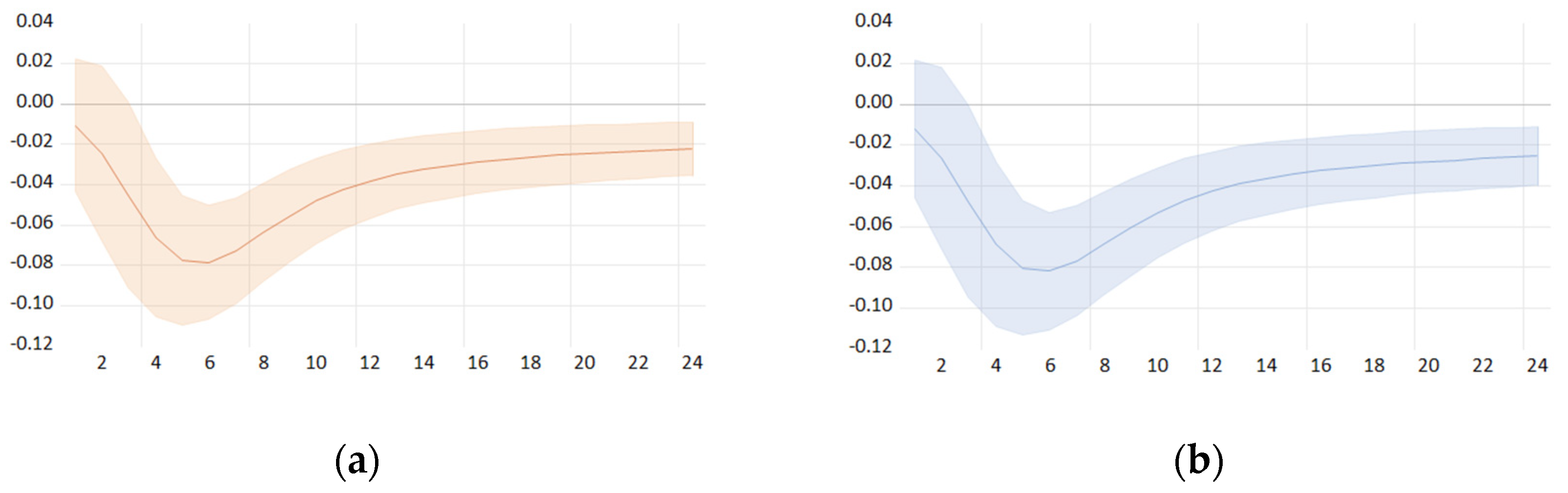
Figure 1 shows the results of the time-invariant VAR analysis. According to the analysis results based on the reduced VAR model comprising the monthly change rates of housing prices, the Composite Index of Business Indicators, and the CD rate, the shock from rising interest rates is found to reduce housing prices.

The reduced VAR model is estimated by configuring the monthly change rates of the Korea Real Estate Board and Kookmin Bank comprehensive housing price indexes as regression equations. The IRF estimation results from the two models are nearly identical. The housing price did not show a statistically significant response within 1 to 2 months of the interest rate shock, and then the price drop was apparent after 3 months and was the largest after 5 to 6 months. These analysis results assume symmetry and invariance, that is, the effects of interest rate shocks are identical at all time points, and the impulse response during periods of rising and falling interest rates are also identical. Thus, the analysis results based on the VAR model assume that the impulse response at all time points is constant, regardless of whether the model form is reduced or structural. This is judged to be a limitation because it assumes that the effects of falling interest rates during a period of past high-interest rates are identical to the effects of falling interest rates during a period of recent low-interest rates. As this analysis assumes that the impulse responses at all time points are the same, the periods of rising and falling interest rates must also be interpreted symmetrically, thereby having limitations in its application.

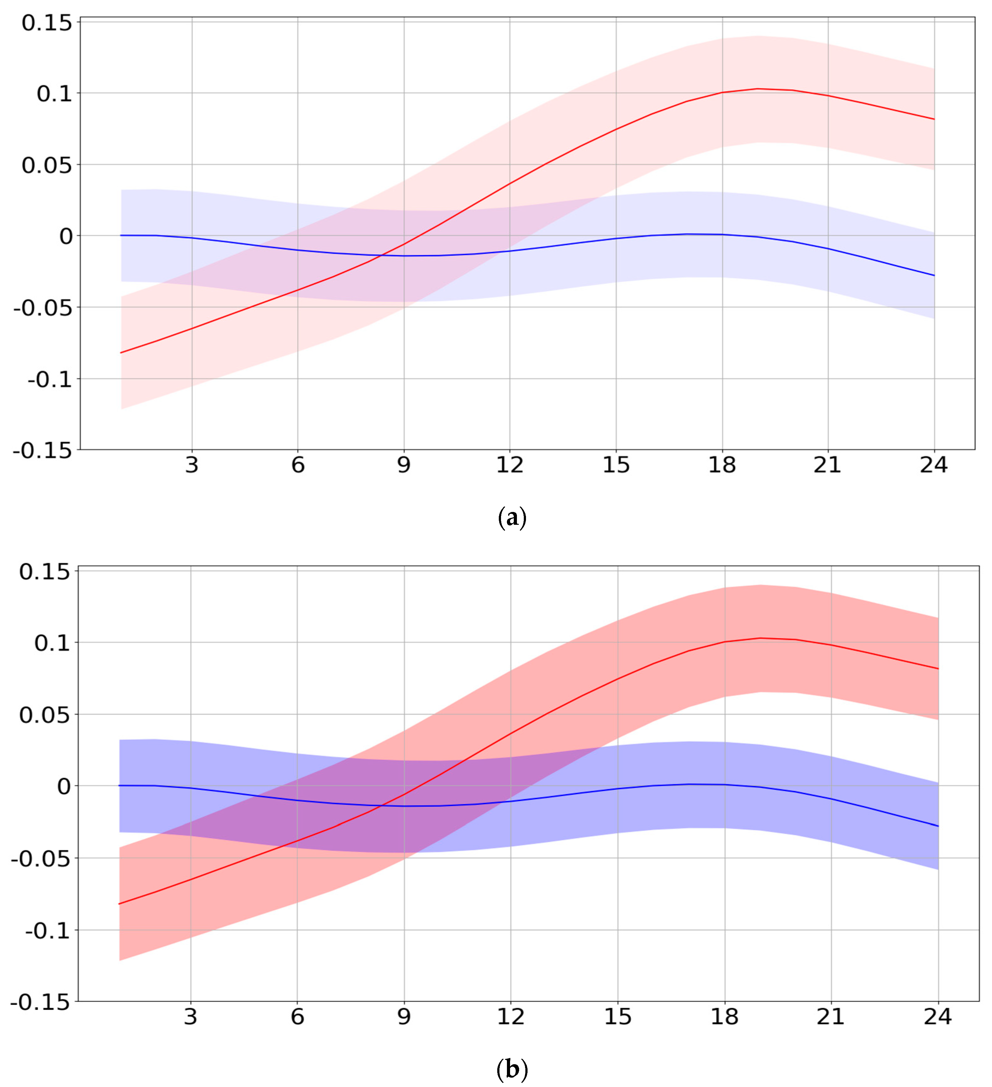
Figure 2 and Figure 3 show the conditional analysis results using the conditional local projection method.

First, we examine the conditional analysis of the period before the global financial crisis in Figure 2. Whereas falling interest rates had no impact on housing prices before the global financial crisis, rising interest rates caused a decline in housing prices in the short term, showing an asymmetry for interest rate shocks. Interest rate shocks during the period of falling interest rates before the global financial crisis did not show a statistically significant effect on housing prices. Interest rate shocks during the period of rising interest rates before the global financial crisis caused housing prices to fall within 6 months; however, the downward pressure on prices did not continue afterward.

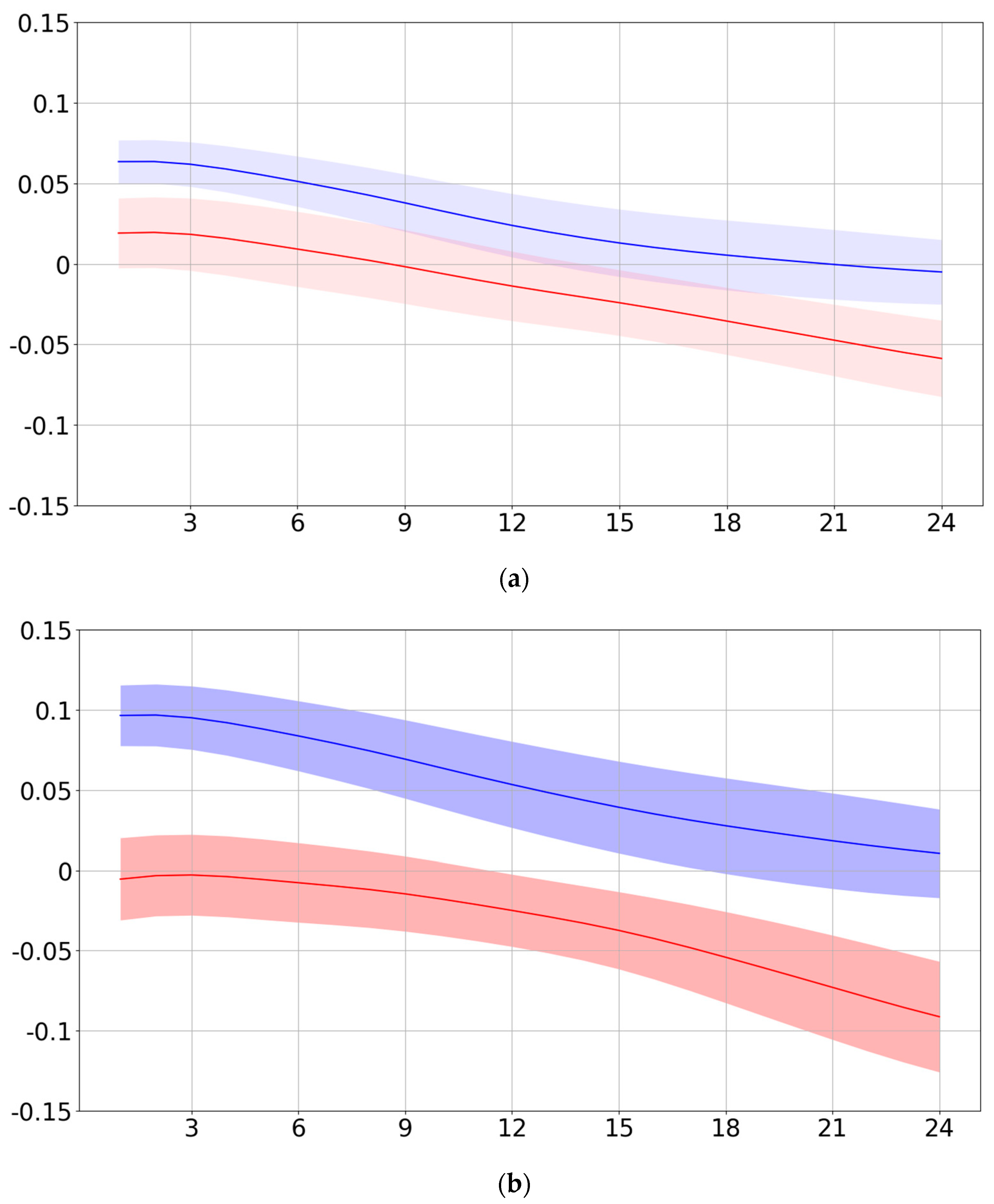
Next, we examine the conditional analysis of the period after the global financial crisis in Figure 3.

After the global financial crisis, the falling interest rates showed a highly elastic influence on housing prices in the short term, whereas rising interest rates showed an influence with a time lag of 12 to 15 months. Thus, the shock from falling interest rates caused housing prices to rise, and this impact lasted for approximately 12 months on the Korea Real Estate Board housing price index and 18 months on the KB housing price index. Owing to the interest rate shock from rising interest rates, the Korea Real Estate Board housing price index showed a falling response after about 15 months, while the KB housing price index showed a falling response after about 12 months.

Next, we examine the analysis results on the time-varying effect of interest rates.

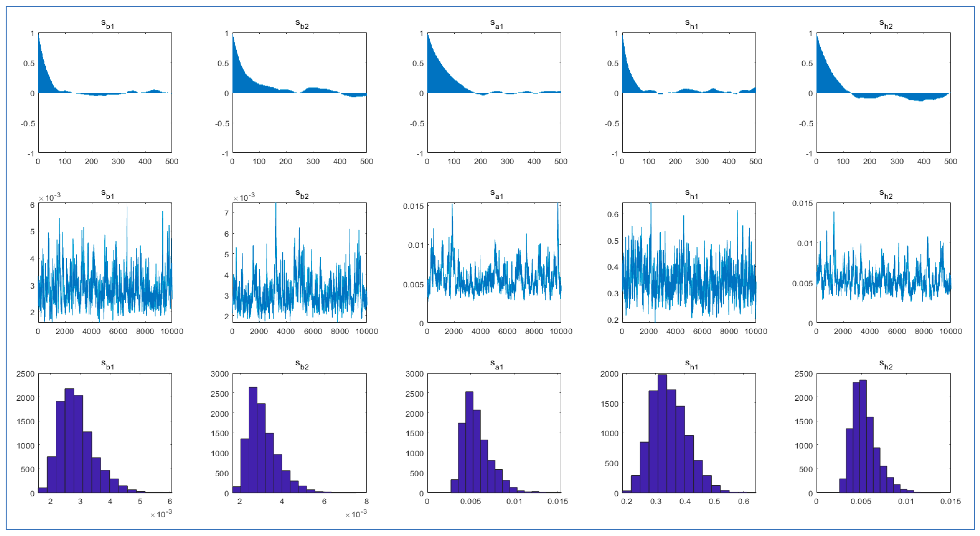
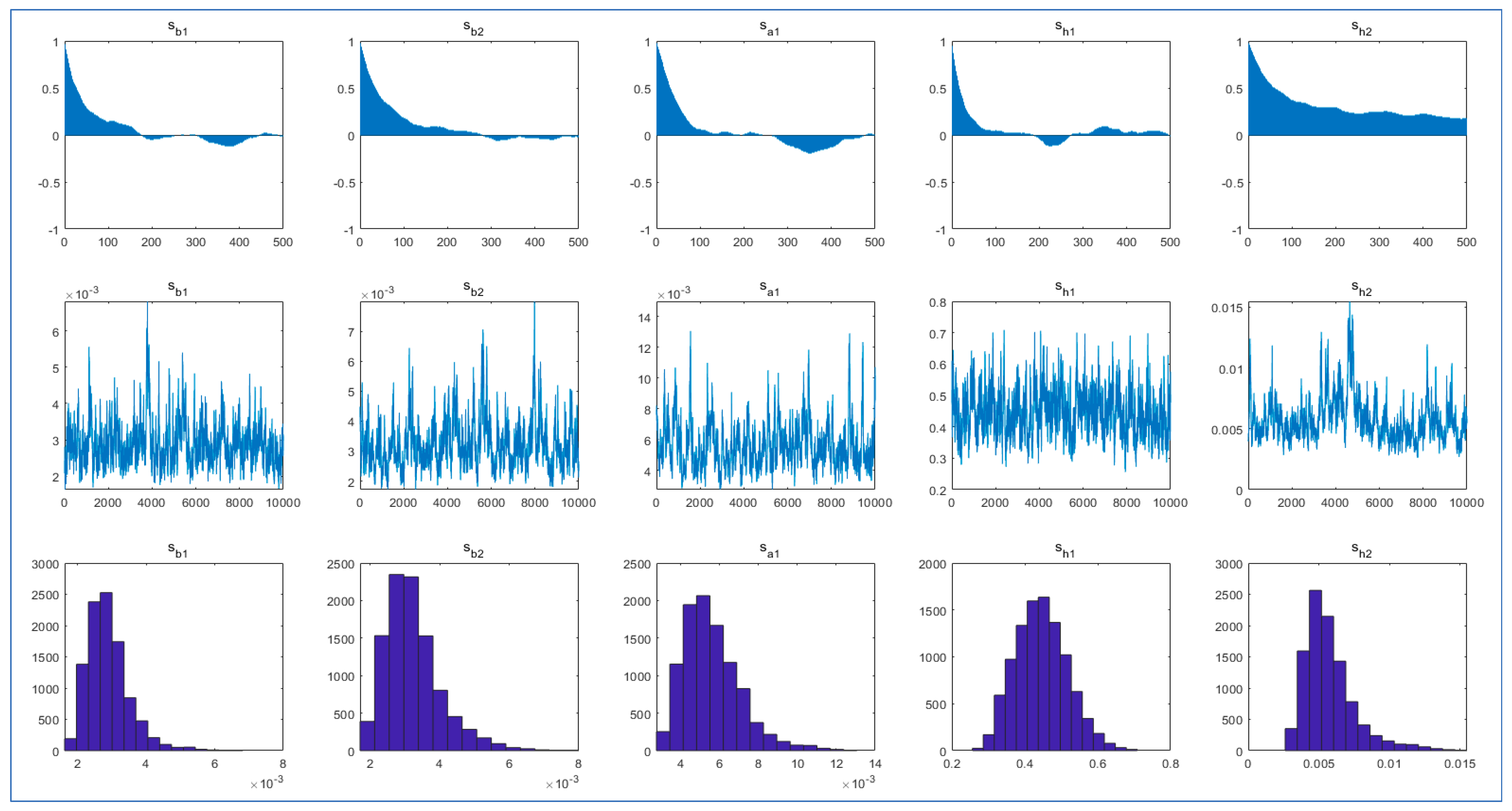
Before reviewing the analysis results, we must first examine the posterior distribution convergence test of the model. To confirm whether the estimates inferred through Gibbs sampling are valid, it is necessary to review the sample autocorrelation, sample path, and posterior distribution density. If the autocorrelation is high in the Gibbs sampling validity test, then the sample path shows a certain pattern, and the posterior distribution may not show the shape of a normal distribution. This suggests that the Markov chain of the constructed model does not converge to the posterior distribution, or even if it does, that sampling is inefficient.

Figure 4 shows the posterior distribution convergence test results on the comprehensive housing data of the Korea Real Estate Board. In the validity test results, the autocorrelation of the first line is initially high but then gradually decreases. The sample path is also repeated around a constant value, and the density function of the posterior distribution does not show an excessive bias, indicating that the Gibbs sampling was properly performed.

The basic idea of the posterior distribution convergence test is presented as follows: if the distribution of the Gibbs sample converges to the posterior distribution, then the sample mean between the given subsamples must match, and when the actual Gibbs sample converges to the posterior distribution, then it converges to the normal distribution according to the central limit theorem.

In

Table 2. Gibbs Sampling Validation Results (based on Korea Real Estate Board Price Index).

Parameter	Mean	SD	95% U	95% L	Geweke	Inefficiency
${\mathrm{S}}_{\mathrm{b}1}$	0.0029	0.0006	0.0020	0.0043	0.682	51.52
${\mathrm{S}}_{\mathrm{b}2}$	0.0031	0.0007	0.0021	0.0049	0.110	89.59
${\mathrm{S}}_{\mathrm{a}1}$	0.0057	0.0017	0.0035	0.0097	0.459	109.27
${\mathrm{S}}_{\mathrm{h}1}$	0.3473	0.0622	0.2420	0.4826	0.092	53.87
${\mathrm{S}}_{\mathrm{h}2}$	0.0054	0.0014	0.0033	0.0088	0.024	75.45

Source: estimated by the authors with the TVP-VAR model.

, the posterior sample extracted via Gibbs sampling shows a normal distribution at the 1~5% significance level. Therefore, the estimated values in this study are efficient, and the distribution of the sample properly converges to the posterior distribution.

Figure 5 shows the posterior distribution convergence test results on the comprehensive housing data of the Kookmin Bank. According to the Gibbs sampling validity test results, the autocorrelation of the first line is initially high but then gradually decreases. However, ${\mathrm{S}}_{\mathrm{h}2}$ shows a relatively high autocorrelation compared to the other parameters. Accordingly, some time series continuity is found in the sample path of ${\mathrm{S}}_{\mathrm{h}2}$. However, the density function of the posterior distribution does not significantly deviate from the general standard normal distribution or show excessive bias.

In

Table 3. Gibbs Sampling Validation Results (based on KB Price Index).

Parameter	Mean	SD	95% U	95% L	Geweke	Inefficiency
${\mathrm{S}}_{\mathrm{b}1}$	0.0029	0.0006	0.0020	0.0044	0.320	79.86
${\mathrm{S}}_{\mathrm{b}2}$	0.0032	0.0008	0.0021	0.0053	0.110	100.16
${\mathrm{S}}_{\mathrm{a}1}$	0.0056	0.0015	0.0034	0.0092	0.060	74.18
${\mathrm{S}}_{\mathrm{h}1}$	0.4455	0.0710	0.3219	0.5942	0.759	48.81
${\mathrm{S}}_{\mathrm{h}2}$	0.0057	0.0018	0.0034	0.0108	0.423	165.98

Source: estimated by the authors with the TVP-VAR model.

, the posterior sample extracted via Gibbs sampling shows a normal distribution at the 5% significance level. Therefore, the sampling in this study is efficient, and the distribution of the sample properly converges to the posterior distribution.

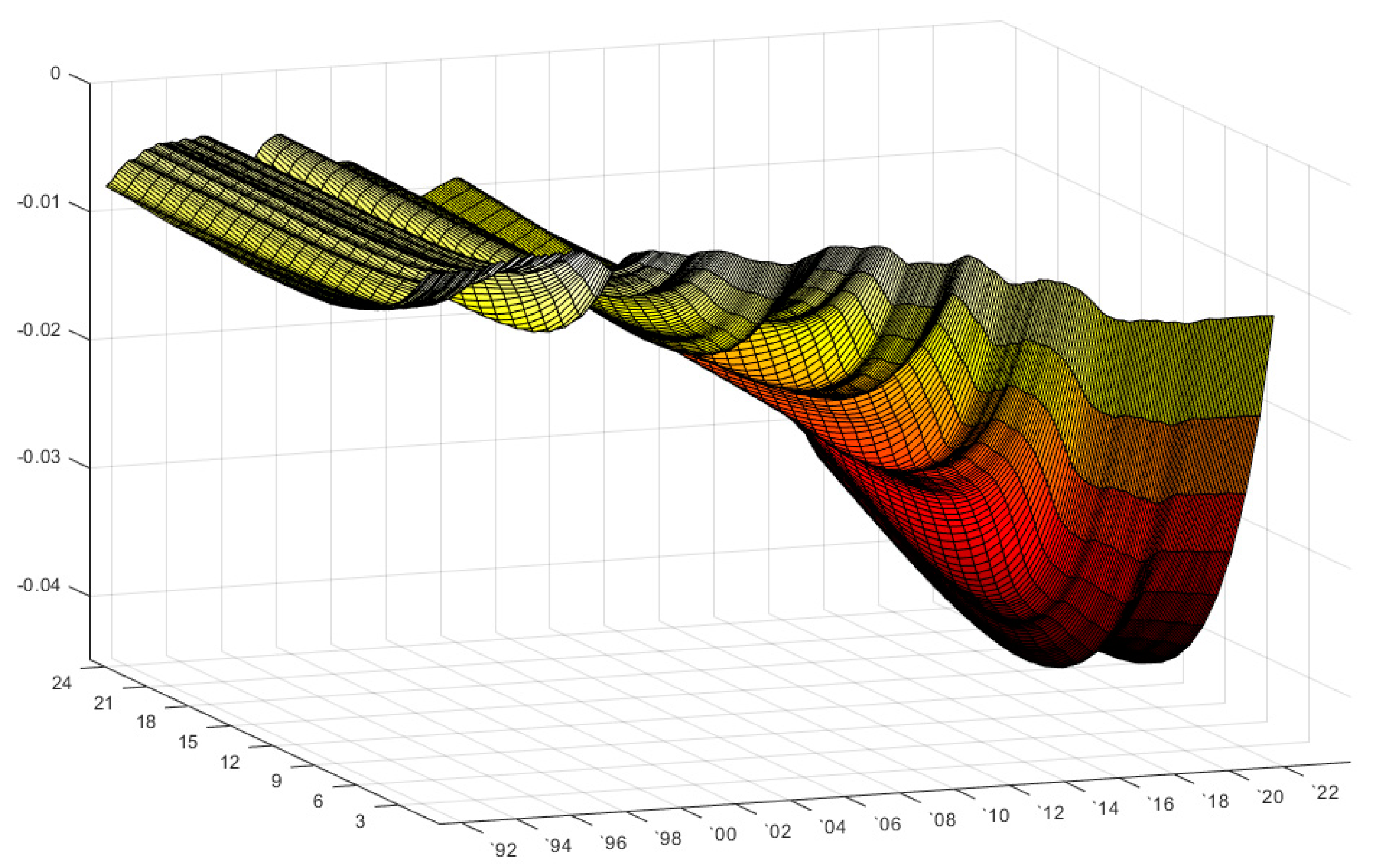
Next, we examine the time-varying estimation results of interest rates on housing prices based on the TVP-VAR model. As shown in Figure 1, the time-invariant IRF adopted in numerous studies on interest rates and housing prices is limited, as it assumes that interest rate shocks at all time points have the same impact on housing prices. Figure 6 and Figure 7 estimate the time-varying IRF through the TVP-VAR model; thus, it is possible to examine how housing prices respond to interest rate shocks over time in the long term.

Figure 6 shows the analysis results based on Korea Real Estate Board comprehensive housing. In the 1990s, housing prices were relatively unaffected even if an interest rate shock occurred, suggesting that a structural break occurred after the global financial crisis in the impact of interest rate shocks on the housing market. Put differently, interest rate changes after the global financial crisis began to have very rapid and strong impacts on the housing market.

This signifies that policies to expand liquidity through interest rates improve consumers’ ability to purchase housing, thus increasing the housing demand in a short period of time and creating an environment to raise housing prices rapidly. Particularly, in the period when the government implemented an accommodative monetary policy after July 2019 to stimulate the real economy, the impact of interest rate fluctuations on housing prices became more severe than in the past.

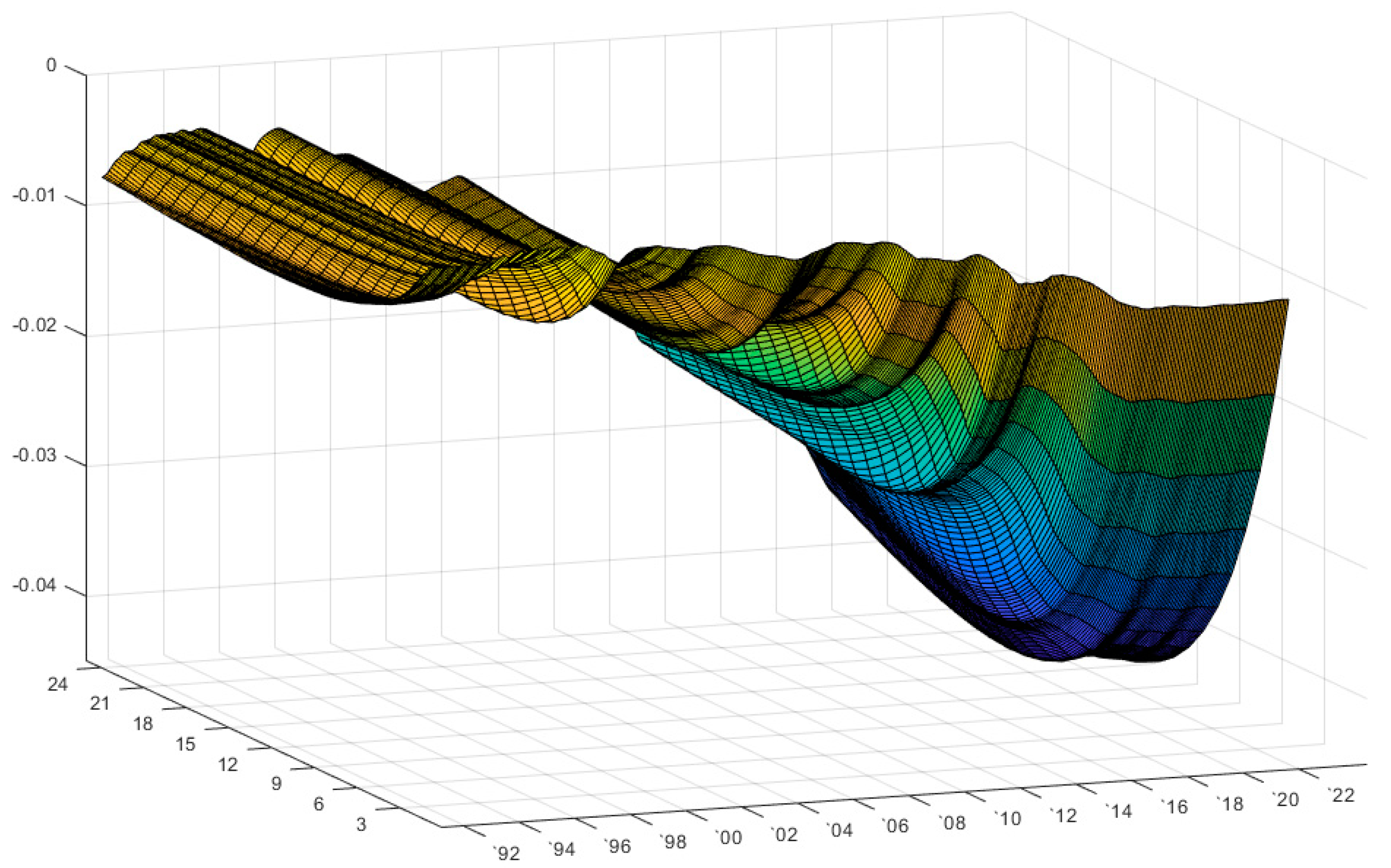
Figure 7 shows the analysis results based on KB comprehensive housing. Almost identical to the findings from Figure 6, the housing market in the past was relatively unaffected by interest rate shocks, whereas recently, the impact of interest rates on the housing market significantly increased.

Based on the characteristics shown in Figure 6 and Figure 7, the structural break in the impact of interest rates on the housing market occurred around 2012. During this period, the government continued the deregulation to stimulate the housing market, which had been stagnant after the global financial crisis.

Specifically, the measures of 22 March 2011 raised the DTI (debt-to-income) ratios and lowered transaction taxes to stimulate transactions. The measures of 10 June 2011 relaxed the period of restriction on purchase right resale in overpopulated constraint districts of the Seoul metropolitan area, as well as the restrictions on the return profit from the reconstruction of old apartments, thus stimulating transactions. The measures of 7 December 2011 abolished the price ceiling system, lifted the regulation on speculative overheat districts, and abolished the heavy capital gains tax on multi-homeowners. The measures of 10 May 2012 raised the LTV (loan-to-value ratio) and DTI ratios in Seoul, exempted the additional capital gains tax rate to homeowners of three homes, expanded the Bogeumjari loan recipient eligibility, and raised its maximum limit, along with raising the loan guarantee limit of the Korea Housing Finance Corporation, thus increasing the demand for the general public. The measures of 10 September 2012 reduced transaction taxes such as capital gains tax and acquisition tax, thus stimulating transactions.

With a growing demand for housing transactions due to such deregulations, the government lowered the base rate in July 2012 and operated an accommodative monetary policy until October 2017. During this period, the impact of interest rates on the housing market significantly expanded.

Next, we divide the results estimated by the TVP-VAR model into periods of falling and rising interest rates and compare the interest rate impulse responses according to the period.

First, in the periods of falling interest rates, the interest rate shocks on housing prices became stronger over time, and the initial response speed, magnitude, and duration all increased (see

Table 4. Analysis of the Cumulative Impulse Response Function of Time Variable at the Time of Interest Rate Cut.

	Based on Korea Real Estate Board Data						Based on KB Data
	P1	P2	P3	P4	P5	P5/P1	P 1	P2	P3	P4	P5	P5/P1
1 month later	0.002	0.003	0.004	0.006	0.010	4.395	0.002	0.003	0.004	0.007	0.010	4.037
3 months later	0.012	0.018	0.023	0.034	0.054	4.426	0.012	0.018	0.024	0.036	0.051	4.124
6 months later	0.034	0.051	0.068	0.098	0.154	4.493	0.034	0.051	0.069	0.104	0.147	4.276
12 months later	0.085	0.130	0.178	0.246	0.394	4.620	0.086	0.130	0.182	0.264	0.388	4.540
24 months later	0.187	0.268	0.393	0.512	0.828	4.415	0.188	0.271	0.408	0.545	0.854

Source: estimated by the authors with the TVP-VAR model.

.). In the fifth period (P5), the most recent period of falling interest rates, the impulse response magnitude significantly increased relative to the previous period. The impulse response magnitude in the fifth period, compared to the first period, increased by more than four times at all the impulse response time points. Thus, it is deemed that the large increase in housing prices from 2020 to 2021 is mainly due to the increased liquidity caused by falling interest rates.

Regarding the periods of rising interest rates, the impulse response in the sixth period of rising interest rates, which began in the second half of 2021, showed a greater magnitude, speed, and duration (see

Table 5. Analysis of the Cumulative Impulse Response Function of Time Variable hen Interest Rates are Raised.

	Based on Korea Real Estate Board Data							Based on KB Data
	P1	P2	P3	P4	P5	P6	P6/P1	P1	P2	P3	P4	P5	P6	P6/P1
1 month later	−0.002	−0.003	−0.003	−0.004	−0.010	−0.010	4.623	−0.002	−0.003	−0.003	−0.005	−0.009	−0.009	4.138
3 months later	−0.011	−0.014	−0.015	−0.024	−0.053	−0.054	4.758	−0.012	−0.014	−0.015	−0.025	−0.049	−0.050	4.320
6 months later	−0.032	−0.041	−0.042	−0.067	−0.151	−0.155	4.869	−0.033	−0.041	−0.044	−0.071	−0.143	−0.147	4.518
12 months later	−0.083	−0.109	−0.112	−0.175	−0.390	−0.402	4.845	−0.084	−0.109	−0.117	−0.188	−0.379	−0.392	4.677
24 months later	−0.176	−0.241	−0.257	−0.419	−0.839	−0.867	4.934	−0.176	−0.241	−0.266	−0.450	−0.847	−0.878

Source: estimated by the authors with the TVP-VAR model.

).

During this period (the current period), the impact of the interest rate shock on the housing market was more severe in the medium and long term than in the short term.

Considering the recent high inflation rate, which requires additional increases to the base rate for a considerable period, downward pressure on housing prices is expected to increase in the future.

5. Conclusions

This paper was written amid steep interest rate hikes in response to worldwide inflation following the low-interest rates which occurred during the COVID-19 pandemic. The recent high inflation rates continue to increase because of expanded liquidity due to ultra-low interest rates near 0% during the previous interest rate cuts, as well as disruptions to the fuel and food supply due to the Russia–Ukraine war. Countries worldwide are raising interest rates in response to inflation. As monetary policy based on interest rates is inelastic, this trend of rising interest rates is expected to continue for a certain period until inflation rates converge to the target levels. As these interest rate hikes are expected to persist, it is necessary to examine the impact of interest rates, which significantly influence the ability to purchase housing.

The empirical work presented here provides one of the first investigations into how the impact of interest rates on housing prices varies depending on the period. For example, in a study that estimated the influence of interest rates on housing prices using the TVP-VAR model, there was no significant evidence in the case of the United States that the interest rates have a strong impact on housing prices [17]. On the other hand, the results from an earlier study [17] demonstrate a strong and consistent association between the interest rates and housing prices in the United Kingdom. Unlike the US and the UK cases, this study in the Korean context, it has been shown that the impact of interest rates on housing prices was not significant in the past, but this trend has been dramatically changed since 2010.

The main analysis results are presented as follows: the interest rates have a negative effect on housing prices; the impact of interest rate shocks on housing prices has expanded since the global financial crisis; and the interest rate shocks during the periods of rising and falling interest rates are asymmetrical.

According to the analysis results using the time-invariant VAR model, which was generally applied in previous studies, the shock of rising interest rates caused housing prices to fall. However, as these analysis results assume that the impulse responses at all time points are the same, they are limited because the periods of rising and falling interest rates must also be interpreted symmetrically.

Based on the conditional local projection method analysis results, whereas falling interest rates had no significant influence on housing prices before the global financial crisis, rising interest rates caused a decline in housing prices in the short term. After the global financial crisis, falling interest rates caused housing prices to rise immediately, whereas rising interest rates caused prices to decline after a time lag of 12 to 15 months. This asymmetry is attributed to the fact that when interest rates fall, demand rapidly grows due to lower financing costs and the expectation for price increases, whereas when interest rates rise, demand and transactions decrease due to increased financing costs.

According to the time-varying VAR analysis results, while the influence of interest rate shocks on housing prices was not large before the global financial crisis, the impact of interest rate shocks on housing prices after the global financial crisis has significantly increased. Particularly, the period of rising housing prices from 2020 to 2021 was found to be when the impact of interest rate shocks was much higher than in the past. Moreover, the interest rate impulse response during the recent period of rising interest rates was found to be much stronger compared to the past. The rise in the impact of interest rate shocks on housing prices is attributed to the increased dependence on loans for housing purchases compared to the past. Hence, a housing market recession is highly likely if interest rate hikes persist.

These analysis results recommend the following tasks.

First, policy measures must be devised to limit the impact of interest rate shocks on the volatility of the housing market. The current impact of interest rate shocks on the housing market is greater than in the past. Housing prices can dramatically rise or fall when trying to achieve a target inflation rate through monetary policy in the medium term. This is because interest rates adjusted based on monetary policy significantly influence the formation of demand in the housing market. As interest rates can cause a high volatility in the housing market, interest rate policies must be accompanied by continuous monitoring and complementary policies to prevent excessive liquidity from flowing into the housing market.

Second, it is necessary to estimate TVP-VAR models for countries that have switched to a low-interest rate system in response to the COVID-19 pandemic, identify their long-term structural break, and conduct comparisons. Major countries lowered their interest rates at similar times in response to the COVID-19 pandemic, during which housing prices rose, and interest rates continued to be increased to fight the subsequent high inflation. It is necessary to analyze these major countries, identify the similarities and differences with the experiences of Korea, and devise measures to reduce the volatility of the housing market.

Third, specific regions must be analyzed while considering the nature of the housing market. Because the scope of this study is nationwide, the analysis results may differ from what is perceived in specific regions. Future studies should conduct region-specific analyses to examine the nonlinearity and time-varying effects of interest rate shocks, such as between Seoul and other regions with high consumer preferences or with relatively low preferences.

References

- Park, J.-B.; Lee, T.-R.; Oh, M.-J. An empirical study on the contribution of interest rates to housing prices. Hous. Policy Stud. 2021, 29, 75–100. [Google Scholar] [CrossRef]
- Yoon, J.-H. Housing Market Diagnosis and Future Prospects. KDI Real Estate Forum. 2021. [Google Scholar]
- Bank of Korea. Korean Monetary Policy Report; Bank of Korea: Seoul, Republic of Korea, 2021. [Google Scholar]
- Seok, B.-H.; You, H.-M. On the Long-Term Effect of Recent Housing Policies in Korea. Korea Econ. Rev. 2021, 37, 199–223. [Google Scholar]
- Lee, C.-M. Critical Assessments on Moon Jae-In Government’s Housing Policies. Korean J. Public Adm. 2020, 29, 37–75. [Google Scholar] [CrossRef]
- Cho, J.-H. Behavioral Economic Understanding of Housing Transaction Price Determination—Focusing on the Formation of Expectations for Apartment Prices; WP 21–19; Korea Research Institute for Human Settlements: Seoul, Republic of Korea, 2021. [Google Scholar]
- Park, J.-B. Estimation of Contribution of Interest Rates before and after Accommodative Monetary Policy to Rise in Housing Prices; WP 21–21; Korea Research Institute for Human Settlements: Sejong, Republic of Korea, 2021. [Google Scholar]
- Primiceri, G.E. Time varying structural vector autoregressions and monetary policy. Rev. Econ. Stud. 2005, 72, 821–852. [Google Scholar] [CrossRef]
- Jordà, Ò. Estimation and inference of impulse responses by local projections. Am. Econ. Rev. 2005, 95, 161–182. [Google Scholar] [CrossRef]
- Son, J.-C. Dynamic analysis of correlations among monetary policy, real and financial variables and housing prices. Hous. Policy Stud. 2010, 58, 179–219. [Google Scholar]
- Jeon, H.-J. Asset pricing theory based on the study on the determinants of housing prices, using VECM. Korea Real Estate Acad. Rev. 2013, 52, 241–255. [Google Scholar]
- Kwon, H.-J.; Yoo, J.-S. Structural changes in metropolitan housing markets and household debt before and after global financial crisis. Korea Res. Ins. Hum. Settl. 2014, 81, 105–119. [Google Scholar]
- Jo, G.-J. Asset price fluctuation and monetary policy. J. Soc. Sci. 2015, 54, 263–281. [Google Scholar] [CrossRef]
- Lee, G.-Y.; Kim, N.-H. Interest rates and housing prices. Korean J. Econ. Stud. 2016, 64, 45–82. [Google Scholar] [CrossRef]
- Lee, Y.-S. Monetary policy and housing market: Bayesian VAR analysis using sign restrictions. Hous. Policy Stud. 2019, 27, 113–136. [Google Scholar] [CrossRef] [Green Version]
- Kang, G.-H. Bayesian Econometrics; Pakyoungsa: Seoul, Republic of Korea, 2016. [Google Scholar]
- Vasilios, P.; Rangan, G.; Constantinos, K.; Mark, E.W. Time-varying role of macroeconomic shocks on house prices in the US and UK: Evidence from over 150 years of data. Empir. Econ. 2020, 58, 2249–2285. [Google Scholar]
Figure 1.
Time-invariant impulse response of housing prices to higher interest rates. (a) Based on the Korea Real Estate Board Price Index, (b) based on KB Price Index. Note: the horizontal axis represents the impulse response period (months), and the vertical axis represents the response (%) to a 1SD interest rate shock. Source: estimated by the authors with the VAR model.
Figure 2.
Conditional impulse response of interest rates before the global financial crisis. (a) Based on Korea Real Estate Board Price Index, (b) based on KB Price Index. Note 1: the horizontal axis represents the impulse response period (months), and the vertical axis represents the response (%) to a 0.25% interest rate shock. Note 2: in the graph, blue indicates the impulse response during a period of falling interest rates, and red the response during a period of rising interest rates. Source: estimated by authors.
Figure 3.
Conditional impulse response of interest rates after the global financial crisis. (a) Based on Korea Real Estate Board Price Index, (b) based on KB Price Index. Note 1: the horizontal axis represents the impulse response period (months), and the vertical axis represents the response (%) to a 0.25% interest rate shock. Note 2: In the graph, blue indicates the impulse response during a period of falling interest rates and red the response during a period of rising interest rates. Source: estimated by authors.
Figure 4.
Post-distribution of Gibbs sampling (based on Korea Real Estate Board Price Index). Note: the first line graph shows the autocorrelation; the second shows the sample path; and the third shows the posterior distribution density. Source: estimated by the authors with the TVP-VAR model.
Figure 5.
Post-distribution of Gibbs sampling (based on KB Price Index). Note: the first line graph shows the autocorrelation; the second shows the sample path; and the third shows the posterior distribution density. Source: estimated by authors with the TVP-VAR model.
Figure 6.
Time-varying impulse response to housing prices (based on Korea Real Estate Board Price Index). Note: X-axis: time of impulse response; Y-axis: magnitude of impulse response; and Z-axis: duration of impulse response. Source: estimated by the authors with the TVP-VAR model.
Figure 7.
Time-varying impulse response to housing prices (based on KB Price Index). Note: X-axis: time of impulse response; Y-axis: magnitude of impulse response; and Z-axis: duration of impulse response (months). Source: estimated by the authors with the TVP-VAR model.