Article

Identifying the Spatiotemporal Transitions and Future Development of a Grazed Mediterranean Landscape of South Greece

by
Dimitrios Chouvardas
,
Maria Karatassiou
*,
Afroditi Stergiou
and
Garyfallia Chrysanthopoulou
Laboratory of Rangeland Ecology (P.O. 286), School of Forestry and Natural Environment, Aristotle University of Thessaloniki, 54124 Thessaloniki, Greece
*
Author to whom correspondence should be addressed.
Land 2022, 11(12), 2141; https://doi.org/10.3390/land11122141
Submission received: 17 October 2022 / Revised: 22 November 2022 / Accepted: 24 November 2022 / Published: 28 November 2022

Abstract

:
Spatiotemporal changes over previous decades in grazed Mediterranean landscapes have taken the form of woody plant encroachment in open areas (e.g., grasslands, open shrublands, silvopastoral areas), altering its structure and diversity. Demographic and socioeconomic changes have played a significant role in landscape transformations, mainly by causing the abandonment of traditional management practices such as pastoral activities, wood harvesting, and agricultural practices in marginal lands. This study aimed to quantify and evaluate the spatiotemporal changes in a typical grazed Mediterranean landscape of Mount Zireia during 1945–2020, and to investigate the effect of these changes on the future development (2020–2040) of land use/land cover (LULC) types. Cartographic materials such as aerial orthophotos from 1945, land use maps of 1960, Corine Land Cover of 2018, and recent satellite images were processed with ArcGIS software. To estimate the future projection trends of LULC types, logistic regression analyses were considered in the framework of CLUE modeling. The results indicated that the strongest trend of spatiotemporal changes were forest expansion in open areas, and grasslands reduction, suggesting that the LULC types that were mainly affected were forest, grasslands, and silvopastoral areas. Future development prediction showed that forests will most probably continue to expand over grassland and silvopastoral areas, holding a high dynamic of expansion into abandoned areas. The reduction in grasslands and silvopastoral areas, independent of environment and biodiversity implications, represents a major threat to sustainable livestock husbandry based on natural grazing resources.

1. Introduction

Mediterranean landscapes are considered highly diverse areas in terms of history, geography and land uses. Several civilizations from ancient times have left a rich cultural heritage promoting this variety [1]. The Mediterranean landscapes, as a result of their long history of human activities, with a unique combination of topographic and climatic variability, have generated a rare combination of unique, but fragile, diverse species-rich ecosystems [2,3]. The Mediterranean basin is the second largest biodiversity hotspot in the world, holding more than 25,000 plant species [4]. The long history of human intervention in this area has formed plant communities that are considered as “man-made” and composed of natural components, a fact that has a significant value in setting goals and methodology for sound conservation interventions [5]. The last 75 years of technological advances, such as the introduction of heavy machinery in farming activities [6], trade globalization, the creation of the European Economic Community [2], and the Common Agricultural Policy (CAP) [7,8], have driven dramatic changes in these ecosystems unlike those experienced in the past [9]. In recent years, climate changes, along with unbalanced land use activities (e.g., coastalization, undergrazing, and land abandonment), have facilitated Mediterranean ecosystems change [10]. Two opposite trends of landscape evolution have occurred in the Mediterranean region in recent decades. Forest cover increased around the northern edge of the Mediterranean region (south European countries) and decreased around its southern edge (mainly in the Maghreb countries). This increase in forest cover in northern Mediterranean landscapes is mainly attributed to the abandonment of marginal agricultural lands [11,12], while the decrease in forest in the south is attributed to the expansion of cropland in marginal areas initially dominated by woodlands [13]. The above changes have followed the socioeconomic trends of land abandonment in rural areas in the north versus the increased population pressure in rural areas in the south [9,14].
One of the main land use activities in Mediterranean landscapes is pastoral activities [2,9,13,15]. Approximately one-fifth of European agricultural lands are dedicated to extensive livestock grazing, with the majority being situated in southern Mediterranean Europe, including the Balkans. Furthermore, 80% of Europe’s sheep and goat flocks are located in Spain, Italy, Greece, and southern France [16]. Grazing is considered a major landscape-changing factor directly related to human activities, especially in Mediterranean areas [17,18]. Greek landscapes have historically been grazed by livestock in quite a similar way as modern practices, and are highly influenced by the changes in traditional pastoral activities [19,20]. Recently, significant changes emerged in the traditional extensive livestock production systems of Greece, mainly related to the reduction in the number of local and transhuman flocks of free-grazing animals (sheep, goats, and cattle) [8,20,21,22,23]. These changes follow the land abandonment trend already mentioned for the European part of the Mediterranean region, and they highly contribute to the spatiotemporal transitions occurring in grazed areas. These transitions are taking the form of woody plant expansion in open areas, transforming grasslands, open shrublands, silvopastoral areas and abandoned agricultural areas, into forest or dense shrublands [21,24,25,26,27,28].
The study of land use/land cover (LULC) change provides an important aspect in understanding the history of spatiotemporal transition patterns, derived from landscape changes. Spatiotemporal transition patterns produce useful data for studying the effect of physical and socioeconomic interactions, land use conflicts, and influences on landscape changes [29,30,31]. Analysis of spatiotemporal changes and transitions is typically conducted within the geographic information systems (GIS) environment [30,32], with visual photointerpretation of a time series set of aerial photographs [33,34] through digital processing of multispectral satellite images [32], or more recently through object-based recognition technics [35]. The development of transition matrices has become an important part of landscape history analysis [36]. New tools and indicators of LULC changes derived from the matrices have emerged, addressing issues related to the annual rate of changes [30], persistence and net changes as quantity difference and swap as allocation difference [37], and identifying systematic or main transitions [29,36].
Predicting the future development of LULC types and transitions is an effective and reliable technique for evaluating both the causes and the significance of past and present conditions, usually under future scenarios [27,38,39]. Several spatiotemporal models for LULC future projections have been proposed over the years [31], including the adoption of empirical models for LULC prediction such as logistic regression approaches (e.g., CLUE modeling framework, LCM, MaxEnt) [39,40,41]. The use of regression analysis in landscape prediction studies contributes to understanding and describing the change mechanisms and processes of LULC types, provides an advanced statistical environment for analyzing multivariate components, and finally, predicts the LULC changes [14,42]. The above prediction models can also produce accurate results to support policy makers, land managers, and scientists in reaching sustainable landscape management decisions [41].
Spatiotemporal changes have a significant effect on altering landscape structure in terms of landscape composition and configuration [43]. These changes can be easily evaluated with the use of landscape metrics [44,45], applied in spatiotemporal studies of landscape changes [22,24,46,47], or in the future projections of land use changes [48].
Overall, there is a limited amount of published information regarding the spatiotemporal changes in grazed landscapes, especially for the eastern part of the Mediterranean region, and particularly about the influences of land abandonment in the future development of land uses that are related to pastoral activities. Therefore, the present research aims to: (a) quantify and evaluate the spatiotemporal changes of a typical, grazed Mediterranean landscape of south Greece (Mt Zireia landscape), (b) investigate the effect of these changes on the future development of the most significant LULC types, and (c) identify their correlation to a set of landscape driving factors. Finally, the overall effect and interactions of socioeconomic changes are explored, focusing on pastoral activities in LULC transitions and future development.

2. Study Area

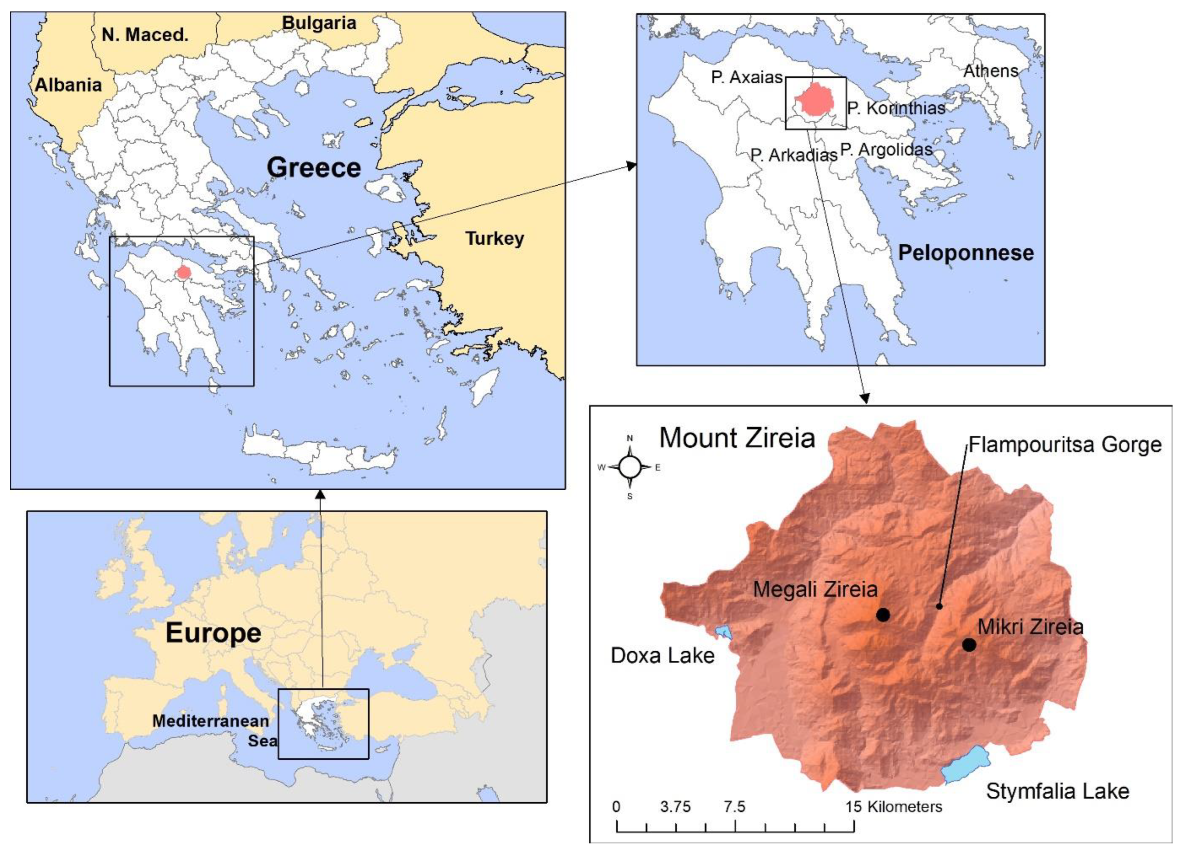
Mount (Mt) Zireia (or Kyllini), located in the Peloponnese peninsula (South Greece), was selected for the study. Mount Zireia is the second highest mountain in the Peloponnese, located in the Korinthos prefecture 115 km west of Athens (Figure 1).
The study area covers 39,762 ha of land inhabiting 3777 people living in 19 village communities–municipalities subdistricts. Elevations in the study range from 310 m to 2374 m a.s.l. A large gorge, called Flampouritsa, divides the mountain into two areas, “Mikri” (small) Zireia and “Megali” (big) Zireia. Mt Zireia, apart from the highest point of 2374 m, has other seven peaks above 2000 m (four in Megali and three in Mikri Zireia). The multiple ridges created by the mountain tops, in combination with valleys and plateaus, create a particularly diverse relief of hills, plains, cliffs, and canyons. More than two-thirds of the study area is part of the network of Natura 2000 protected areas (pSCI, SCI or SAC, SPA) [49]. Two main hydrological basins are found in the area, creating the natural lake Stymfalia (area 15,285 ha) to the south, and the artificial lake Doxa (area 48 ha) in the west (Figure 1), which greatly affect the microclimatic conditions and facilitate the touristic development of the area. Lake Stymfalia is closely connected to Greek mythology, and especially with Heracles’ legendary labors. According to mythology, the lake was full of aggressive man-eating Stymphalian birds, and Heracles’ sixth labor was to exterminate them [50].
The climate, according to Köppen–Geiger climate classification, is a hot summer Mediterranean climate (coded as “Csa”) [51]. The mean annual precipitation has varied over the last 60 years, from 418.62 mm (in 1993) to 1056 mm (in 2005), while the mean annual temperature varied from 12.59 °C (coldest year in 1976) to 15.55 °C (warmest year in 2010) [52].
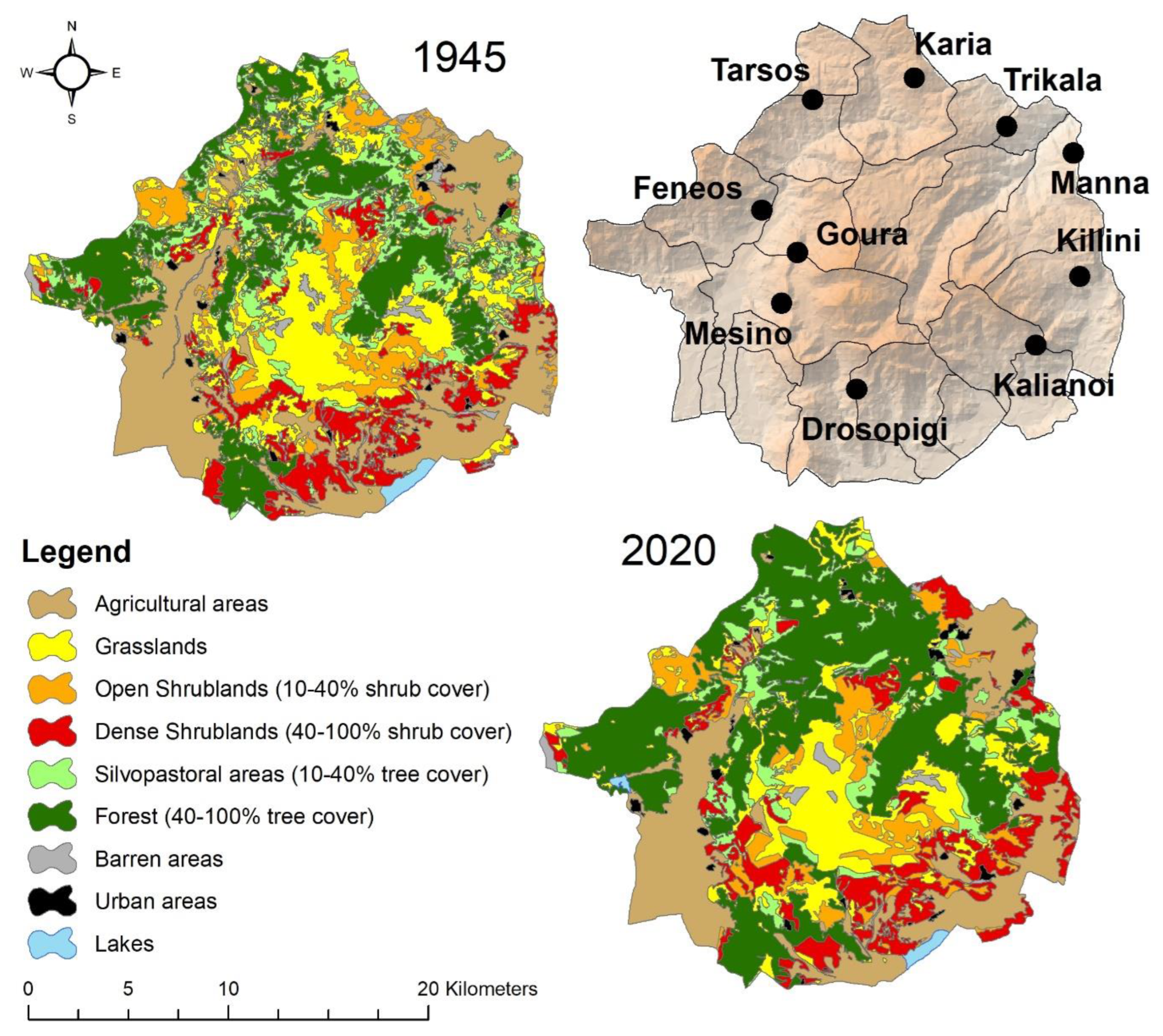
The main land uses of the area are forests, rangelands, and agricultural areas. Rangelands include grasslands, shrublands, and silvopastoral areas with less than 40% tree cover and grazed by sheep and goats. Agricultural areas are cultivated mainly with annual crops such as beans, corn, barley, and wheat [52].
According to the official census report derived from the Hellenic Statistical Authority [53], the temporal evolution of socioeconomic data from 1961 (oldest available data) until the most recent available data of 2011, showed that in the last 50 years, the total population, active workforce, and employees in the primary economic sector has rapidly been reducing (Table 1), following the general trend of land abandonment that many researchers have reported for the Mediterranean region [8,44,54,55]. Age structure analysis indicates that the human population is becoming older. Indeed, 62% of the population was under 44 in 1961, versus 47% in 2011 (Table 2).
In contrast, the local population over 45 years old increased from 38% to 53%, for the same period. The above data are in line with demonstrated demographic change in the Mediterranean region and the movement of the mainly younger population from rural areas to urban centers [8,11,44].
Census data from the Hellenic Statistical Authority and the Payment and Control Agency for Guidance and Guarantee Community Aid [56], regarding the historical data of transhumans [57], revealed that the number of grazing animals (mainly sheep and goats) and their farms have significantly reduced in the last 50 years (Table 3) [20].
The total number of grazing animals decreased from 1961 to 2011 by 38% (Table 3). This reduction was more intensive for transhuman animals (more than 64%) and less for sedentary animals (almost 4%). According to the available inventory data, the number of sedentary animal farms significantly reduced by 80% during a similar period (Hellenic Statistical Authority, 1961 to 2000). This reduction follows the similar trend of change as the number of people that are employed in the primary sector of the economy (Table 1).

3. Materials and Methods

3.1. Land Use/Land Cover Changes. Spatiotemporal Transitions

The following cartographic materials (Figure 2) were considered: (a) digital aerial orthophotographs of 1945 with a spatial resolution of 1 m obtained from the National Cadastre of Greece (georeferenced to the Hellenic Geodetic Reference System 1987-HGRS87); (b) satellite images obtained from the Google Earth Pro program for the years 2017, 2019 and 2020 (georeferenced to HGRS87); (c) maps of forest vegetation and land cover for 1960 (scale 1:20,000), obtained from the Ministry of Agriculture in digital format (shapefile in HGRS87); and, (d) digital maps of Corine Land Cover 2018 (shapefile reprojected in HGRS87).
Aerial orthophotographs from 1945, as well as the recent Google Earth satellite pictures, were digitally processed using the software ArcGIS v.10.8.1, to produce LULC maps for 1945 and 2020. To identify the distinct LULC types, on-screen visual photointerpretation and manual delineation of LULC polygons in shapefile format were performed within the ArcGIS environment (Figure 2). The chosen analysis used a classification scheme consisting of eight categories of LULC types and was based on the Greek Forest Service’s LULC classification system (Table 4). According to the chosen classification system, numerous elements on aerial orthophotos and Google Earth images were recognized by using common photographic keys (tone, texture, pattern, shade, form, and size) and feature association [15,21,29,33,34]. Special attention was placed on identifying tree and shrub cover density patterns with the use of crown density scales [58]. The 1960 forest vegetation and land cover maps in shapefile format were a valuable resource for the 1945 LULC mapping, since they served as a reference map and guided the photointerpretation. The minimum mapping unit of the reference map was one hectare, and the same unit was chosen for the 1945 and 2020 mappings. For the 2020 LULC mapping, additional supporting materials were considered from the 2018 Corine Land Cover digital map, and from several elements of the Google Earth application software, such as 3D views and street view images available from many narrow-paved roads between villages of the study area. The visual interpretation was also supported by field sampling verifications from well-experienced human image interpreters with good knowledge of the area. The above cartographic materials were further processed using ArcGIS and Excel to create tables and digital maps of the temporal evolution of LULC types. This approach produced two digital maps of LULC types for 1945 and 2020, as well as a temporal evolution table (Figure 2).
According to Puyravad [59], the annual rate of change of LULC types was calculated for the overall study period (1945–2020). The annual rate calculation Equation (1) was based on the formula developed from compound interest law, and offers a better assessment and biological meaning to the LULC change comparisons because it is insensitive to the different time periods between observation dates [29]:
r = 1 t 2 t 1 × ln A 2 A 1
where r is the annual rate of change, and A1 and A2 are the LULC class areas at time t1 and t2, respectively.
The next phase in the process was to estimate the spatiotemporal transformations of the study area for 2020 as a result of the diachronic transitions of all LULC types from their original surfaces in 1945. This was accomplished by employing a common post-classification comparison (PCC) change detection method across the study’s periods of various dates [30]. The PCC method produced a LULC change transition matrix, which was calculated using ArcGIS overlay functions for all time periods. In addition, a map showing the spatiotemporal transition of LULC types was constructed. Additional components of land changes, such as gains and losses, net changes, total changes, and swap [60], were included in the LULC changes study due to transition matrices. The proportion of the landscape that underwent gross gain or loss of LULC type j between times 1 and 2 was represented by the letters P+j and Pj+, respectively. The proportion of the landscape that demonstrated the persistence of category j was indicated by the diagonal elements (denoted as Pjj) of LULC types [60]. The difference between gain and loss is called net change and was denoted as Dj. Swap is the simultaneous gain and loss of LULC type j, and was calculated as two times the minimum gain and loss (Sj). The sum of the net change and the swap, or the sum of gains and losses for each LULC type j, abbreviated as Cj, is the total change [29,60]. In order to calculate net changes, swaps, and total changes, Equations (2)–(4) were applied:
D j = P + j P j +
  S j = 2 × M I N   P j + P j j ,   P + j   P j j
  C j   = D j + S j
Recent scientific views have defined net change as quantity difference (or quantity disagreement), and swap as allocation difference (or allocation disagreement) [37].
Identification of the most systematic transitions or dominant signals of change is another critical component in evaluating LULC alterations [29,61]. The most important form of transition can be determined using the transition matrix data by adding the total area of change for each LULC type over the time periods. This technique cannot consider the random process of LULC changes caused by the dominant LULC types and, therefore, interpreting LULC transitions based on their sizes is the correct way to evaluate them [29]. The predicted gains (denoted as Gij) and expected losses (denoted as Lij) that will occur if random changes among the LULC types occur, were computed using a process that was first proposed by Pontius [61] (Equations (5) and (6)):
G i j = P + j P j j P i + 100 P j +
L i j = P i + P i i P + j 100 P + i
The difference between the observed (Pij) and expected (Gij or Lij) transitions in a random process of gain (PijGij) or loss (PijLij) is indicated as Dij, and the ratios meaning (PijGij)/Gij or (PijLij)/Lij are denoted as Rij. Dij and Rij values show the tendency of a LULC type j to gain from type i (focus on gains) and the tendency of LULC type i to lose from type j (focus on losses) [60]. Systematic transitions or dominant signals of change are indicated by values having a considerable positive or negative deviation from zero [29]. Rij ratios are equivalent to the (observed value − expected value)/expected value ratios that are used in chi-square tests [61].
The results from the annual rate of change, absolute values of net change, and the main systematic transitions of all LULC types were used to identify the main LULC types that had undergone significant spatiotemporal changes.

3.2. Logistic Regression, Probability Maps, and Future Projection

The future projection trends of the main LULC types that were identified as experiencing the most significant spatiotemporal changes, were determined by logistic regression analyses, under the methodological approach of the CLUE modeling framework [21,62,63,64,65]. According to CLUE modeling, a set of landscape driving factors (LDF were used as independent variables in the regression analysis. In this research, 20 LDF variables were identified and collected based on the physiographic, accessibility, and socioeconomic conditions of the study area (Table 5).
In addition to the above independent variables, the identified main LULC types were selected as dependent variables. According to the spatial module of the CLUE model, both the LULC types and the independent variables were transformed into digital raster files (ArcGrid format) with a pixel size of 100 m. The raster files of all dependent variables and 8 out of 20 independent variables (Table 5) were binarily rendered. As a result, each pixel of a given main LULC type and the eight independent variables received a value of 1, and those without received a value of 0. All the other independent variables received a continuous value according to their definition. The raster data sets were then transformed into ArcGIS ASCII grids, and with the use of the “File Convert v2” application of Dyna-CLUE modeling version [64], were further transformed into tabular format necessary for entry in the SPSS statistical package v. 27.0 (IBM Corp., Armonk, NY, U.S.A.).
In SPSS, the data were analyzed by the method of binary logistic regression of absence/presence, using forward conditional analysis as a step-by-step regression method. The input and output probabilities of the independent variables in the equation were set to not surpass the significance levels of input = 0.01 and output = 0.02, respectively, during the process [64]. Variables that did not meet the above criteria were rejected as exhibiting a low degree of correlation to the model. This procedure resulted with fewer independent variables from the original selection, and resolved problems due to multicollinearity [66,67,68]. The regression coefficients (bi) of the remaining independent variables in the logistic equation were tabulated. Furthermore, the area under the ROC (relative operating characteristic) curve (AUC) was estimated, as a measure of controlling the goodness of fit of the data to the logistic regression model [64,69], and was used to validate the model (Figure 2) [65,70].
The AUC number indicates how well the model can differentiate across classes [71,72]. The greater the value, the better the model’s ability to distinguish between classes. AUC values range from 0 to 1, with 0.5 indicating that the model is unable to distinguish between the classes, and 1 indicating that the model is perfectly fitted [73,74,75]. AUC levels of 0.7 to 0.8 are considered acceptable, 0.8 to 0.9 are considered excellent, and values beyond 0.9 are considered exceptional [76,77]. All the available data concerning the dependent and independent variables and the logistic regression results from SPSS were introduced into the Dyna-CLUE version of the model, to produce a set of land use probability maps. Probability maps represent the distribution of the results of the logistic regression equations in the landscape [64].
The land use demands for 2040 of the identified main LULC types that have undergone significant spatiotemporal changes were computed using linear interpolation of their historical trend (Figure 2). This technique is often used to construct “Business as Usual” model scenarios (BAU scenario) [27,62]. The BAU scenario for a 20-year prediction period (2020–2040) was calculated by adding one-third of the total positive or negative trend of change from the most recent available historic trend, which were the years 1960 and 2020 (60-year trend). The areas of identified main LULC types for 1960 were obtained from the available forest vegetation and land cover map. As Mamanis and coworkers [27] suggested, the one-third ratio was used because the 20-year prediction period is equal to a third of the historical trend (20 years/60 years = 1:3). The projected land use demands under the BAU scenario were spatially allocated into the probability maps based on the higher probability of occurrences, which resulted in the creation of the predicted potential map of the future distribution of the main LULC types. The 2040 prediction maps did not consider LULC interactions.
Finally, the projected results were examined using the ArcGIS Patch Analyst program [21,45,78,79,80]. The number of patches (NumP) and mean patch size (MPS, ha) as overall measures of landscape fragmentation, edge density (ED, m/ha) as a measure of the number of ecotones [44], and mean nearest neighbor (MNN, m) as a measure of patch isolation, were calculated as indicators of spatial heterogeneity in landscape and class levels. The mathematical formulas for the specified indices can be found in the user manuals for Patch Analyst and Arc Fragstats [45,78,79].

4. Results

4.1. Land Use/Land Cover Changes. Spatiotemporal Transitions

The results of photo interpretation and LULC changes over the 75-year periods in terms of area, percentage, and annual rate of changes are shown in Table 6. The LULC types that increased in the study area were forest (68%), dense shrublands (10%), and urban areas (41%) (Table 6).
All the other LULC types decreased, with the more important changes being the reduction in silvopastoral areas (39%), grasslands (27%), and agricultural areas (16%) (Table 6). Open shrublands were reduced in area to a limited extent (5%). Barren areas and lakes were also reduced by 45% and 5%, respectively, but they covered only a limited part of the study area. Forest and dense shrubland expansion, at the expense of silvopastoral areas, grasslands, and agricultural areas, demonstrated that in the last 75 years, woody vegetation in the study area had significantly increased. Analyzing in more detail the annual rate of changes of LULC types (Table 6) during the study period 1945–2020, suggested that the most significant changes were the declining trend of barren areas, silvopastoral areas, and grasslands, and the increasing trend of forest and urban areas. Agricultural areas presented a considerable declining trend, but were less severe compared with grasslands and silvopastoral areas.
Gradual conversion of silvopastoral areas and grasslands into forest was observed in the northern areas between the villages of Feneos, Tarsos, Karya, and Trikala (Figure 3). Forest also seemed to have expanded in the southern area near the village of Drosopigi at the expense of shrubland areas. Grasslands decreased over time in the study areas, except for the central area east of the village Goura, where a higher elevation of landscape occurs (>1200 m). Changes in agricultural areas did not have a strong spatiotemporal orientation, suggesting that they covered a broader range of landscape territories.
The LULC transition matrix of the study area showed that between 1945 and 2020, 65.71% of the total landscape remained unchanged, while 34.29% was transformed into a different LULC type (Table 7). According to the matrix, the most important LULC transitions (>2%) were those of silvopastoral areas (SI) into forest (FO); of grasslands (GR) into open shrublands (OS), silvopastoral areas (SI) and forest (FO); and finally, of dense shrublands (DS) into forest (FO). Additional significant changes (1–2%) were presented in agricultural area transition into grasslands (GR) and shrublands (open, OS; or dense, DS); and open shrublands (OS) transition into dense shrublands (DS) and forest (FO). The results of the matrix suggested that the most important changes in the Mt Zireia landscape were woody plant encroachment into open areas such as grasslands, open shrublands, and silvopastoral areas, and to a lesser extent, into agricultural areas (Table 7).
Figure 4 presents the map of LULC transitions in the study area. It is notable that silvopastoral and forest expansions were mainly located in the northern parts of the study area. On the other hand, shrubland expansions were mainly observed in the southern and central parts of the landscape. Overall, LULC transitions were observed in all parts of the Zireia landscape, but appeared to be more extensive in the northern parts.
The most significant changes in net values (absolute values) were observed in forest, grasslands, and silvopastoral areas, and to a lesser extent, in agricultural areas (Table 8). These data also indicated that the highest losses in the area were observed in grasslands and silvopastoral areas, and the highest gains in forest areas. Net change values in forest were much higher than in comparison with their swap values, suggesting that forest expansion in new areas (quantity difference) was more significant than their simultaneous exchange of forest areas to other uses (allocation difference). On the contrary, net change and swap value changes appeared to be more balanced in grasslands and silvopastoral areas. Forest, grasslands, and silvopastoral areas were the main LULC types that underwent significant changes, and the recorded woody plant expansion in the landscape focused particularly on forest development (Table 8).
Table 9 presents the percentage of the area of the main systematic transitions of LULC changes in terms of gains and losses. The largest positive or negative variation from zero (systematic transitions) appeared to be in the transitions of silvopastoral to forest (SI to FO), grasslands to silvopastoral (GR to SI), grasslands to open shrublands (GR to OS), and open to dense shrublands (OS to DS). These results suggested that forest was systematically gaining area from silvopastoral areas, while dense shrublands gained from open ones (focus on gains). On the other hand, the same results showed that grasslands were systematically losing areas to open shrublands and silvopastoral areas (focus on losses).
Overall, spatiotemporal changes in the landscape of Mt. Zireia indicated that the most important element of landscape change was the woody plant expansion into open areas. Furthermore, among the different LULC types, the ones that were mainly affected by landscape changes were forest, grasslands, and silvopastoral areas in terms of area, percent, and the annual rate of changes (Table 6), the absolute value of net change (Table 8) and the main systematic transitions (Table 9).

4.2. Logistic Regression, Probability Maps and Future Projection of Forest, Grasslands and Silvopastoral Areas

The logistic regression analyses (forward conditional–stepwise) revealed the influence of each of the 20 included independent variables on the LULC types of forest, grasslands, and silvopastoral areas (dependent variables). The area under the ROC curve (AUC) is presented in Figure 5.
AUC values for the three main LULC types were above 0.8 for forest and grasslands, which is accepted as an excellent discrimination, and 0.697 (equal to almost 0.7) for silvopastoral areas, which is marginally acceptable discrimination [77], indicating that the logistic regression models possessed significant goodness of fit.
The b-values of the independent variables are presented in Table 10. The cells without data indicate the independent variables which did not show a statistically significant correlation with the LULC types. The regression coefficients of Table 10 (b-values and constant) were entered into the CLUE software environment to build a set of three probability maps and finally complete the landscape change prediction procedure. The produced maps of the probability (%) of future occurrence for forest, grasslands, and silvopastoral areas in the study area are presented in Figure 6.
According to the probability maps (Figure 6), forest possessed a higher possibility of occurrence mainly in the north-northwest parts of the study area, and to a lesser extent, in a restricted area in the south. Grasslands, on the other hand, were found to be highly possible to occupy areas of high altitude in the center part of the study region, covering the grounds of the sub-alpine zones near Mt Zireia’s summit. Silvopastoral areas received a lower chance of occurrence compared with forest and grasslands, and these chances of occurrence were scattered around the landscape.
Land use demands of the three LULC types under the BAU scenario for a 20-year prediction period (2020–2040), are presented in Table 11. According to Table 11, if the main factors of change (landscape changing factors–independent variables) continue to be the same between 2020 and 2040, then forest is expected to increase in some areas by 15%, and grasslands and silvopastoral areas to decrease by 11% and 31%, respectively.
Spatial allocation of the projected land use demands into the probability maps (Figure 6) produced the predicted potential map (Figure 7) of the spatiotemporal distribution for forest, grasslands and silvopastoral areas for the 2020–2040 period. Forest is expected to continue expanding in the north-northwest parts, and probably will occupy scattered new areas in the central parts of the landscape. The projected grasslands reduction, on the other hand, will most probably force the remaining grassland patches to be limited to the central parts of the landscape. Silvopastoral areas will probably continue to occupy small, scattered areas around the landscape, but with a spatial distribution uneven in size.
The above results can be confirmed by evaluating the landscape structure of the projected maps with the help of landscape metrics (Table 12). According to the metrics during the projected period (2020–2040), the expansion of forests will probably increase their overall fragmentation in the sense that numerous new and smaller sized patches (indicated by the NumP and MPS values) will be created in new areas across the landscape (Table 12). That increase will improve the ED value, creating new forest edges and promoting forest connectivity, as was indicated by the decrease in their MNN value.
Grassland patches, on the other hand, will probably become smaller in size (decrease in MPS value) and distant from each other, as was indicated by the increase in their MNN value. The latter observation will probably promote patch isolation of the smaller grassland units which occupy the marginal areas around their main distribution in the center of the landscape (Figure 7). Furthermore, the decrease in ED value indicates that a significant reduction in grasslands ecotone is to be expected. Silvopastoral patches are expected to become more fragmented in the future, meaning greater in numbers but smaller in size (indicated by the NumP and MPS differences). Moreover, even though silvopastoral areas would increase their overall connectivity (MNN value), they are expected to greatly reduce their edges (ED value), similar to grasslands.

5. Discussion

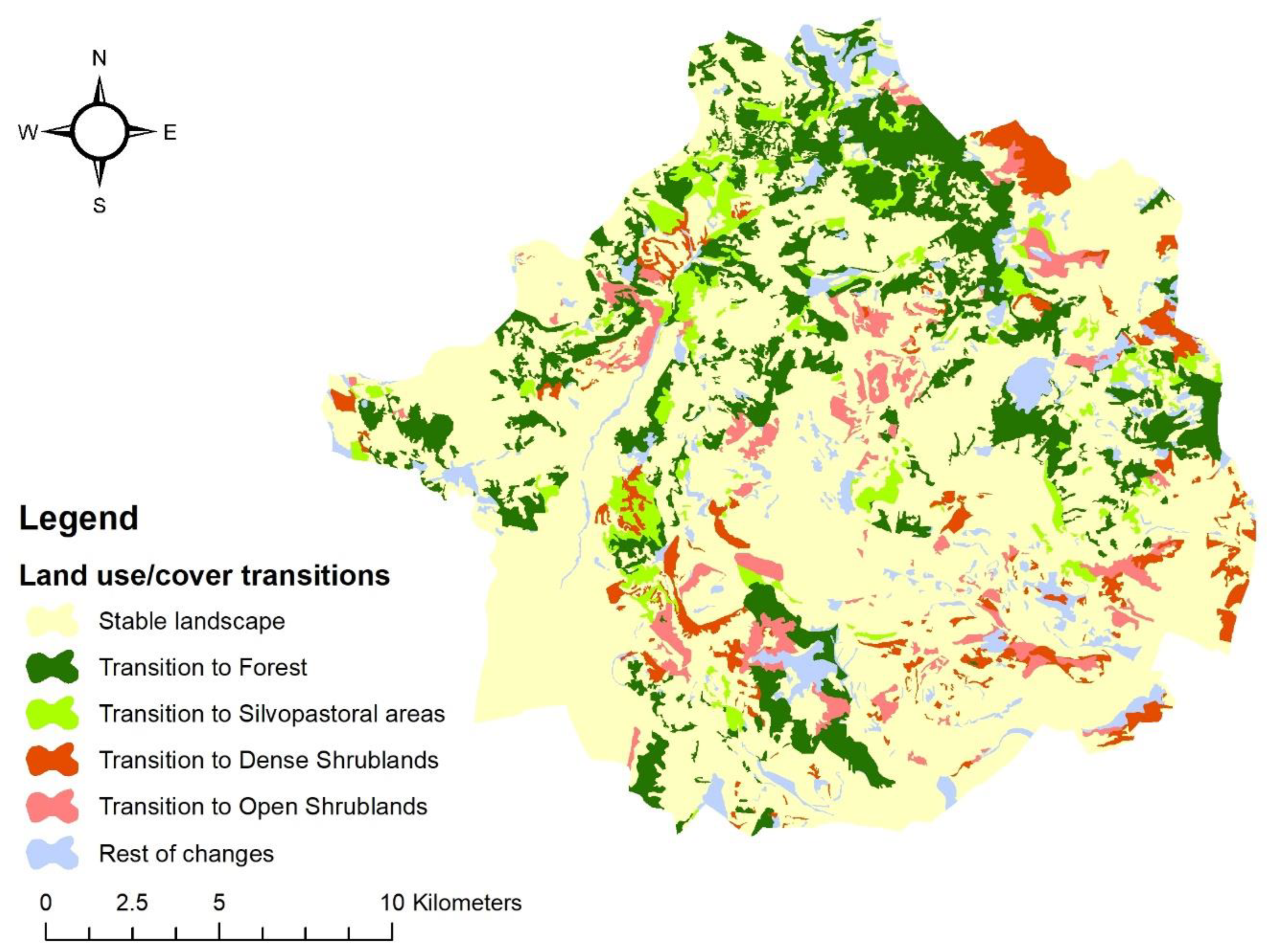
Spatiotemporal transition analysis of the landscape of Mt Zireia suggested that the strongest trend of landscape evolution was woody plant expansion in open areas, and grasslands reduction. Among the different LULC transitions, the most systematic ones (Table 9) were forest expansion over silvopastoral areas, of open shrublands over dense shrublands, and of grassland reduction in favor of open shrublands and silvopastoral areas. These results, combined with the data of the total LULC changes in area, percent, and the annual rate and net changes (Table 6 and Table 8), suggested that the LULC types that are mainly affected by landscape changes are forests, grasslands and silvopastoral areas. This finding, especially as far as the forest expansion/grasslands reduction trend is concerned, is in line with similar studies conducted in Greece [15,24,25,28] and other Mediterranean countries [2,47,55,81], indicating that special focus should be provided to these specific LULC interactions, especially in the rapidly-changing Mediterranean landscapes [9].
The above trend of LULC interactions can mainly be attributed to land abandonment issues related to socioeconomic conditions. Relevant inventory data from the village communities in the study area (Table 1 and Table 2) suggested that socioeconomic changes over the previous decades in the study area had the form of a decrease in local population, population aging and a significant temporal reduction in the percentage of employees in the primary economic sector. These specific types of socioeconomic changes are reported to especially occur in Mediterranean landscapes, as directly related to the abandonment of traditional management practices, such as extensive or semi-extensive pastoral activities (including transhumance pastoralism), wood product collection (e.g., coal and fuel woods) and agricultural practices in less favorable areas (e.g., crop fields in terraces) [8,47,54,55,81,82,83].
Additional inventory data related to the numbers and farms of grazing animals from the study area supports the notion that land abandonment has affected pastoral activities (Table 3 and Table 4). More specifically, the number of sedentary and transhumant grazing animals and farms for the study area were significantly reduced over the previous decades, following a similar trend of change as the number of people that were employed in the primary sector of the economy. The reduction in grazing animals was also reported to follow a similar, more general, trend of reduction for the whole country and for other south European Mediterranean countries [8,11,81]. The collection of forest products seems to be affected by the abandonment of traditional practices. Unpublished data from the PACTORES Project (www.pactores.eu (accessed on 10 December 2021)) indicated that fuel wood collection by local people within the study area has significantly reduced over the years, and in some areas has practically stopped. On the other hand, some of the forest expansion over open areas can be attributed to the afforestation policies of the local forest service to increase the area covered by high forests. Finally, agricultural activities were also affected by land abandonment, but this effect was less severe on the extent of agricultural lands. According to the spatiotemporal analysis of this research, agricultural areas scored as the fourth most important LULC change in terms of total area, percent of change, annual rate, and net changes (Table 6 and Table 8) and these changes did not appear to have a strong geographic orientation (Figure 3). Agricultural activities were mainly oriented in plains in favorable and more accessible parts of the Mt Zireia landscape, which, as similar studies have pointed out, are probably less affected by land abandonment [11,84]. All these aspects of socioeconomic effects in the current management of Mediterranean landscapes have been noted throughout the Mediterranean region of Europe [2,13,15,22,24,25,54,55,81,85] and have been identified as the main reasons for landscape change.
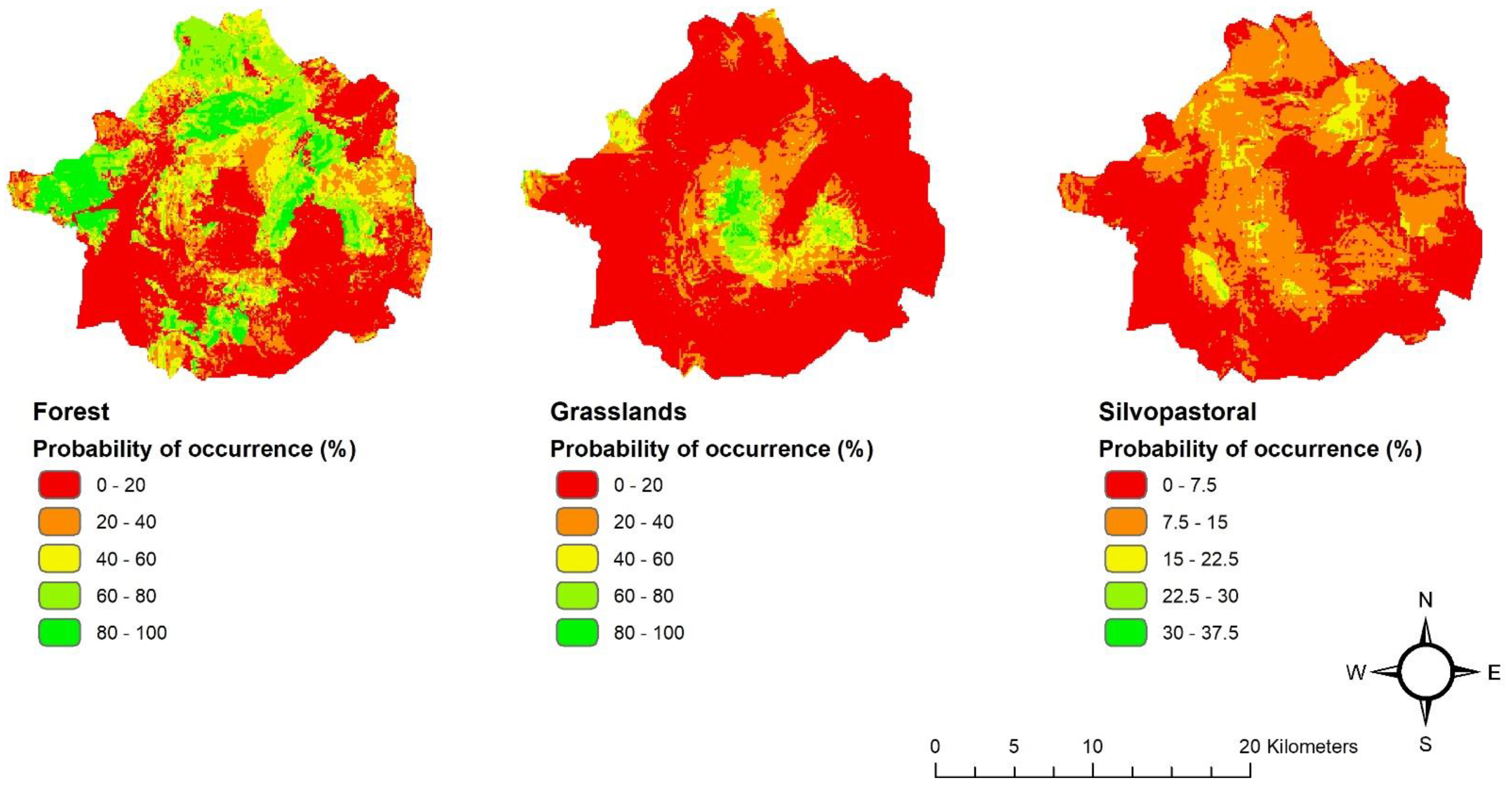
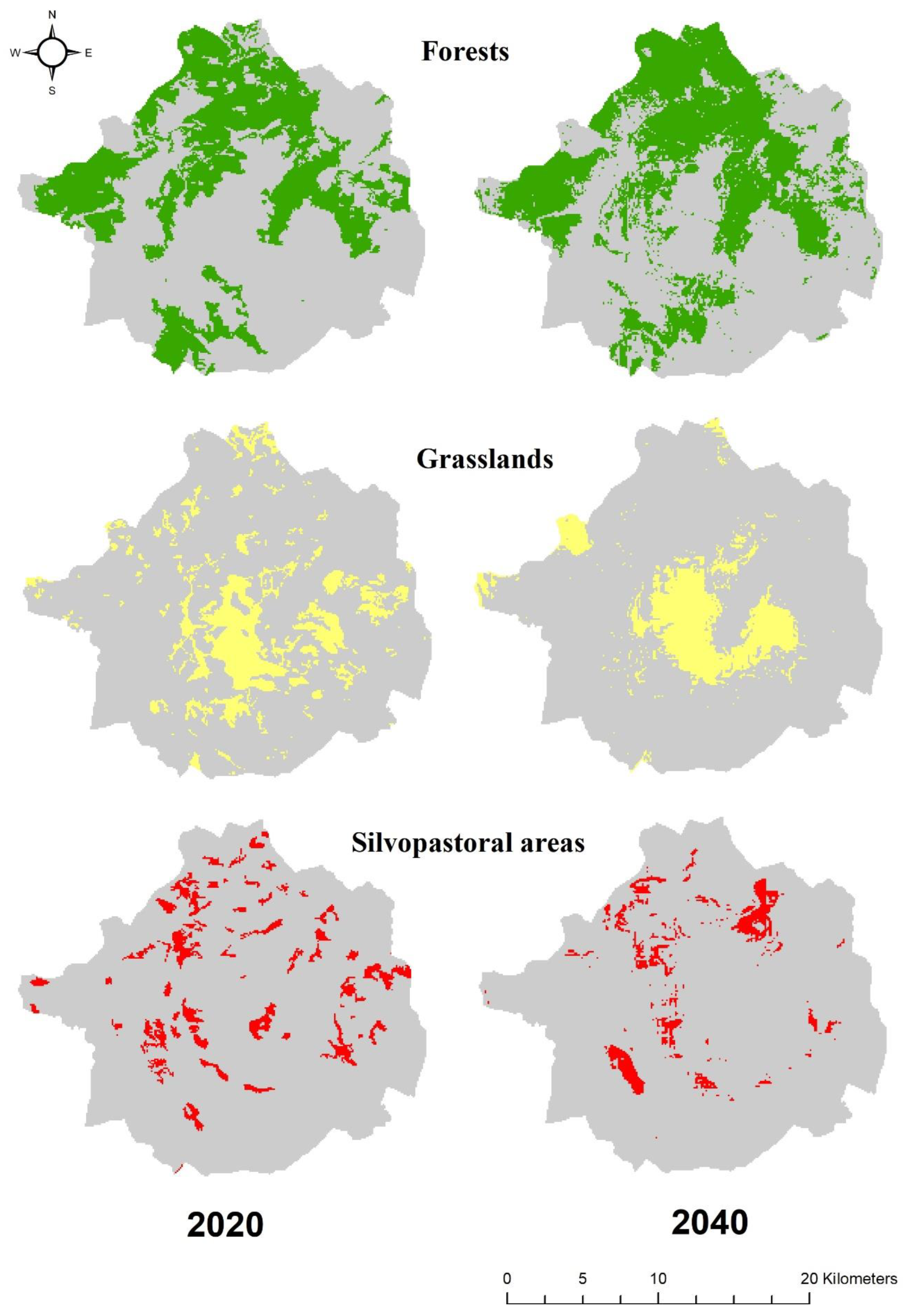
Future development for forest, grasslands, and silvopastoral areas based on the BAU scenario of linear extension of land use demands for 2040 and probability maps, suggested that forest will most probably continue to expand in the north-northwest parts, adding new areas scattered mainly in the central parts of the landscape. At the same time, grassland and silvopastoral areas will probably continue to reduce in area, occupying territories mainly at the central part for grasslands, or small scattered territories around the landscape for silvopastoral areas (Figure 7). Similar results of future development of forests and grasslands were very recently reported from a rural landscape study of central Greece under a similar trend of land abandonment [27,65]. Evaluation of the structural developments (Table 12) of the Mt Zireia landscape from the projected maps revealed that forest expansion into new areas, and in many cases, as small patches, will increase their overall dispersal and will create new forest edges (higher ED value). Furthermore, the decrease in MNN value will promote forest connectivity. Grasslands, on the other hand, apart from occupying one large and three smaller core areas in the center and the north-northwest part of the study area (Figure 7), will probably keep only smaller, fragmented, and isolated patches around the landscape, as indicated by the reduction in their MPS and the increase in their MNN values. Moreover, the decrease in ED value will cause a significant reduction in grassland edges. Silvopastoral patches, similar to grasslands, will became more fragmented with reduced edges. These findings correlate with the response of many other landscapes around the world, showing that forest expansion usually leads to increased forest patch connectivity promoting forest edges, while open habitat reduction usually creates the opposite trend of a reduction in connectivity and edges [86,87]. These results could be alarming for sustaining the environmental integrity of the Mt Zireia landscape, as many researchers have linked grasslands fragmentation and the loss of connectivity and boundary lengths of open habitats, to the decline of species richness and mountainous biodiversity [47,86,88]. The results of landscape metrics evaluation on the future development of LULC types can serve as evidence of the great dynamic of expansion that forest patches possess over grassland and silvopastoral patches, independent of the environment and biodiversity implications.
The findings of this study are consistent with the common pattern of woody cover expansion over open regions in many Mediterranean landscapes that suffer from land abandonment [89]. Environmental integrity, biodiversity, and cultural heritage may be positively or negatively impacted by land abandonment, which can additionally benefit forest ecosystems by fostering it at minimal cost and on a larger scale [65]. Forest recovery promotes carbon sequestration, erosion reduction, and several other ecosystem services such as climate and water regulation, wood production, and recreation [12]. On the other hand, land abandonment, especially in the Mediterranean region, results in declining biodiversity and loss of traditional cultural landscapes [7,81,84], and is often linked to an increased risk of wildfires and decreased river flows [83,90,91]. The land abandonment effect can also be associated with the loss of important cultural elements and services related to traditional pastoral activities, such as cultural heterogenic pastoral landscapes, gastronomical heritage, and folklore elements [92,93].
Developmental planning must take into consideration the spatiotemporal trends and the future projection of LULC types recorded in this study. Forest expansion over grassland and silvopastoral areas, apart from the environmental and cultural implications, would have a strong negative effect on the future of sustainable development of livestock husbandry in the study area. Grassland and silvopastoral areas are considered important natural resources necessary for applying extensive pastoral practices, especially the transhuman livestock system, and the reported threat status could have a damaging effect on keeping the ecological integrity and the social benefits that people expect from pastoral landscapes [62,94,95].

Author Contributions

Conceptualization, D.C. and M.K.; methodology, D.C., M.K., A.S. and G.C.; software, D.C. and A.S.; validation, D.C., M.K., A.S. and G.C.; formal analysis, D.C., M.K., A.S. and G.C.; investigation D.C., M.K., A.S. and G.C.; resources, D.C. and M.K.; data curation, D.C., M.K., A.S. and G.C.; writing—original draft preparation, D.C., M.K. and A.S.; writing—review and editing. D.C., M.K. and A.S.; visualization, D.C., M.K., A.S. and G.C.; supervision, M.K.; project administration, M.K.; funding acquisition, M.K. All authors have read and agreed to the published version of the manuscript.

Funding

This research was part of the project «PACTORES» and was co-funded by the European Union (European Social Fund, ERANETMED2-72-303) and General Secretariat for Research and Innovation (GSRI, Τ8ΕΡΑ2-00022) through the Action “ERA-Net”.

Data Availability Statement

The data presented in this study are available in figures and tables provided in the manuscript.

Conflicts of Interest

The authors declare no conflict of interest.

References

  1. Sluiter, R.; de Jong, S.M. Spatial patterns of Mediterranean land abandonment and related land cover transitions. Landsc. Ecol. 2007, 22, 559–576. [Google Scholar] [CrossRef]
  2. Sirami, C.; Nespoulous, A.; Cheylan, J.-P.; Marty, P.; Hvenegaard, G.T.; Geniez, P.; Schatz, B.; Martin, J.-L. Long-term anthropogenic and ecological dynamics of a Mediterranean landscape: Impacts on multiple taxa. Landsc. Urban Plan. 2010, 96, 214–223. [Google Scholar] [CrossRef]
  3. Marignani, M.; Chiarucci, A.; Sadori, L.; Mercuri, A.M. Natural and human impact in Mediterranean landscapes: An intriguing puzzle or only a question of time? Plant Biosyst. 2016, 151, 900–905. [Google Scholar] [CrossRef]
  4. Ecosystem, C. Ecosystem Profile: Mediterranean Basin Biodiversity Hotspot. Critical Ecosystem Partnership Fund. BirdLife Int. 2017, 309. Available online: https://www.cepf.net/sites/default/files/mediterranean-basin-2017-ecosystem-profile-english_0.pdf (accessed on 23 November 2022).
  5. Perevolotsky, A. Integrating landscape ecology in the conservation of Mediterranean ecosystems: The Israeli experience. Isr. J. Plant Sci. 2005, 53, 203–213. [Google Scholar] [CrossRef]
  6. Papanastasis, V. Traditional vs contemporary management of Mediterranean vegetation: The case of the island of Crete. J. Biolog. Res. 2004, 1, 39–46. [Google Scholar]
  7. Delattre, L.; Debolini, M.; Paoli, J.C.; Napoleone, C.; Moulery, M.; Leonelli, L.; Santucci, P. Understanding the Relationships between Extensive Livestock Systems, Land-Cover Changes, and CAP Support in Less-Favored Mediterranean Areas. Land 2020, 9, 518. [Google Scholar] [CrossRef]
  8. Nori, M.; Farinella, D. Migration, Agriculture and Rural Development: IMISCOE Short Reader; Springer Nature: Berlin/Heidelberg, Germany, 2020. [Google Scholar]
  9. Papanastasis, V.P. Land Use Changes. In Mediterranean Mountain Environments; John Wiley & Sons: Hoboken, NJ, USA, 2012; pp. 159–184. [Google Scholar] [CrossRef] [Green Version]
  10. Guarino, R.; Vrahnakis, M.; Rojo, M.P.R.; Giuga, L.; Pasta, S. Grasslands and shrublands of the Mediterranean region. In Encyclopedia of the World’s Biomes; Goldstein, M., DellaSala, D., Eds.; Elsevier: Amsterdam, The Netherlands, 2020; Volume 3, pp. 635–638. [Google Scholar]
  11. Levers, C.; Müller, D.; Erb, K.; Haberl, H.; Jepsen, M.R.; Metzger, M.J.; Meyfroidt, P.; Plieninger, T.; Plutzar, C.; Stürck, J.; et al. Archetypical patterns and trajectories of land systems in Europe. Reg. Environ. Chang. 2015, 18, 715–732. [Google Scholar] [CrossRef]
  12. Nocentini, S.; Travaglini, D.; Muys, B. Managing Mediterranean Forests for Multiple Ecosystem Services: Research Progress and Knowledge Gaps. Curr. For. Rep. 2022, 8, 229–256. [Google Scholar] [CrossRef]
  13. Peñuelas, J.; Sardans, J. Global Change and Forest Disturbances in the Mediterranean Basin: Breakthroughs, Knowledge Gaps, and Recommendations. Forests 2021, 12, 603. [Google Scholar] [CrossRef]
  14. Millington, J.D.A.; Perry, G.; Romero-Calcerrada, R. Regression Techniques for Examining Land Use/Cover Change: A Case Study of a Mediterranean Landscape. Ecosystems 2007, 10, 562–578. [Google Scholar] [CrossRef]
  15. Papanastasis, V.P.; Chouvardas, D. Application of the state-and-transition approach to conservation management of a grazed Mediterranean landscape in Greece. Isr. J. Plant Sci. 2005, 53, 191–202. [Google Scholar] [CrossRef] [Green Version]
  16. Nori, M. Redressing Policy Making in Pastoral Areas of the Mediterranean Region. J. Policy Gov. 2022, 2, 21–32. [Google Scholar] [CrossRef]
  17. Glasser, T.; Hadar, L. Grazing management aimed at producing landscape mosaics to restore and enhance biodiversity in Mediterranean ecosystems. Options Méditerr. 2014, 109, 437. [Google Scholar]
  18. Psyllos, G.; Hadjigeorgiou, I.; Dimitrakopoulos, P.G.; Kizos, T. Grazing Land Productivity, Floral Diversity, and Management in a Semi-Arid Mediterranean Landscape. Sustainability 2022, 14, 4623. [Google Scholar] [CrossRef]
  19. Hadjigeorgiou, I. Past, present and future of pastoralism in Greece. Pastor. Res. Policy Pract. 2011, 1, 24. [Google Scholar] [CrossRef] [Green Version]
  20. Karatassiou, M.; Parissi, Z.M.; Stergiou, A.; Chouvardas, D.; Mantzanas, K. Patterns of transhumant livestock system on Mount Zireia, Peloponnese, Greece. Opt. Mediterr. Ser. A 2021, 126, 197–200. [Google Scholar]
  21. Chouvardas, D. Estimation of Diachronic Effects of Pastoral Systems and Land Uses in Landscapes with the Use of Geographic Information Systems (GIS). Ph.D. Thesis, School of Forestry and Natural Environment, Aristotle University of Thessaloniki, Thessaloniki, Greece, 2007. [Google Scholar]
  22. Sidiropoulou, A.; Karatassiou, M.; Galidaki, G.; Sklavou, P. Landscape Pattern Changes in Response to Transhumance Abandonment on Mountain Vermio (North Greece). Sustainability 2015, 7, 15652–15673. [Google Scholar] [CrossRef] [Green Version]
  23. Ragkos, A.; Abraham, E.M.; Papadopoulou, A.; Kyriazopoulos, A.P.; Parissi, Z.M.; Hadjigeorgiou, I. Effects of European Union agricultural policies on the sustainability of grazingland use in a typical Greek rural area. Land Use Policy 2017, 66, 196–204. [Google Scholar] [CrossRef]
  24. Zomeni, M.; Tzanopoulos, J.; Pantis, J.D. Historical analysis of landscape change using remote sensing techniques: An explanatory tool for agricultural transformation in Greek rural areas. Landsc. Urban Plan. 2008, 86, 38–46. [Google Scholar] [CrossRef]
  25. Sklavou, P.; Karatassiou, M.; Parissi, Z.; Galidaki, G.; Ragkos, A.; Sidiropoulou, A. The Role of Transhumance on Land Use /Cover Changes in Mountain Vermio, Northern Greece: A GIS Based Approach. Not. Bot. Horti Agrobot. Cluj-Napoca 2017, 45, 589–596. [Google Scholar] [CrossRef] [Green Version]
  26. Rapti, D.; Chouvardas, D.; Parissi, Z. Study of Temporal Evolution of Olympus Landscape. In Proceedings of the 9th Panhellenic Rangeland Congress, Larisa, Greece, 9–12 October 2018; pp. 82–89. [Google Scholar]
  27. Mamanis, G.; Vrahnakis, M.; Chouvardas, D.; Nasiakou, S.; Kleftoyanni, V. Land Use Demands for the CLUE-S Spatiotemporal Model in an Agroforestry Perspective. Land 2021, 10, 1097. [Google Scholar] [CrossRef]
  28. Nasiakou, S.; Chouvardas, D.; Vrahnakis, M.; Kleftoyanni, V. Temporal Changes Analysis of Mouzaki’s Landscape, Western Thessaly, Greece (1960–2020). In Proceedings of the 10th Panhellenic Rangeland Congress, Florina, Greece, 4 March 2022; pp. 147–152. [Google Scholar]
  29. Teferi, E.; Bewket, W.; Uhlenbrook, S.; Wenninger, J. Understanding recent land use and land cover dynamics in the source region of the Upper Blue Nile, Ethiopia: Spatially explicit statistical modeling of systematic transitions. Agric. Ecosyst. Environ. 2013, 165, 98–117. [Google Scholar] [CrossRef]
  30. Munthali, M.; Botai, O.; Davis, N.; Abiodun, A. Multi-temporal Analysis of Land Use and Land Cover Change Detection for Dedza District of Malawi using Geospatial Techniques. Int. J. Appl. Eng. 2019, 14, 1151–1162. [Google Scholar]
  31. Abbas, Z.; Yang, G.; Zhong, Y.; Zhao, Y. Spatiotemporal Change Analysis and Future Scenario of LULC Using the CA-ANN Approach: A Case Study of the Greater Bay Area, China. Land 2021, 10, 584. [Google Scholar] [CrossRef]
  32. Attri, P.; Chaudhry, S.; Sharma, S. Remote Sensing & GIS based Approaches for LULC Change Detection—A Review. Int. J. Curr. Eng. Techn. 2015, 5, 3126–3137. [Google Scholar]
  33. Carta, A.; Taboada, T.; Müller, J.V. Diachronic analysis using aerial photographs across fifty years reveals significant land use and vegetation changes on a Mediterranean island. Appl. Geogr. 2018, 98, 78–86. [Google Scholar] [CrossRef]
  34. Kiziridis, D.A.; Mastrogianni, A.; Pleniou, M.; Karadimou, E.; Tsiftsis, S.; Xystrakis, F.; Tsiripidis, I. Acceleration and Relocation of Abandonment in a Mediterranean Mountainous Landscape: Drivers, Consequences, and Management Implications. Land 2022, 11, 406. [Google Scholar] [CrossRef]
  35. Feizizadeh, B.; Alajujeh, K.M.; Lakes, T.; Blaschke, T.; Omarzadeh, D. A comparison of the integrated fuzzy object-based deep learning approach and three machine learning techniques for land use/cover change monitoring and environmental impacts assessment. GIScience Remote Sens. 2021, 58, 1543–1570. [Google Scholar] [CrossRef]
  36. Zhang, B.; Zhang, Q.; Feng, C.; Feng, Q.; Zhang, S. Understanding Land Use and Land Cover Dynamics from 1976 to 2014 in Yellow River Delta. Land 2017, 6, 20. [Google Scholar] [CrossRef] [Green Version]
  37. Cribari, V.; Strager, M.P.; Maxwell, A.E.; Yuill, C. Landscape Changes in the Southern Coalfields of West Virginia: Multi-Level Intensity Analysis and Surface Mining Transitions in the Headwaters of the Coal River from 1976 to 2016. Land 2021, 10, 748. [Google Scholar] [CrossRef]
  38. Verburg, P.H.; Overmars, K.P.; Huigen, M.G.A.; de Groot, W.T.; Veldkamp, A. Analysis of the effects of land use change on protected areas in the Philippines. Appl. Geogr. 2006, 26, 153–173. [Google Scholar] [CrossRef]
  39. Mas, J.-F.; Kolb, M.; Paegelow, M.; Olmedo, M.T.C.; Houet, T. Inductive pattern-based land use/cover change models: A comparison of four software packages. Environ. Model. Softw. 2014, 51, 94–111. [Google Scholar] [CrossRef] [Green Version]
  40. Amici, V.; Marcantonio, M.; La Porta, N.; Rocchini, D. A multi-temporal approach in MaxEnt modelling: A new frontier for land use/land cover change detection. Ecol. Inform. 2017, 40, 40–49. [Google Scholar] [CrossRef]
  41. Nwaogu, C.; Benc, A.; Pechanec, V. Prediction Models for Landscape Development in GIS. In Dynamics in GIscience; Ivan, I., Horak, J., Inspektor, T., Eds.; Springer International Publishing AG 2018: Cham, Switzerland, 2018; pp. 289–304. [Google Scholar]
  42. Minetos, D.; Polyzos, S. Multivariate statistical methodologies for testing hypothesis of land-use change at the regional level. A review and evaluation. J. Environ. Prot. 2009, 10, 834–866. [Google Scholar]
  43. Feng, Y.; Liu, Y.; Tong, X. Spatiotemporal variation of landscape patterns and their spatial determinants in Shanghai, China. Ecol. Indic. 2018, 87, 22–32. [Google Scholar] [CrossRef]
  44. Farina, A. The Cultural Landscape as a Model for the Integration of Ecology and Economics. Bioscience 2000, 50, 313–320. [Google Scholar] [CrossRef] [Green Version]
  45. McGarigal, K. FRAGSTATS Help; University of Massachusetts: Amherst, MA, USA, 2015; Volume 182. [Google Scholar]
  46. Kumar, M.; Denis, D.M.; Singh, S.K.; Szabó, S.; Suryavanshi, S. Landscape metrics for assessment of land cover change and fragmentation of a heterogeneous watershed. Remote Sens. Appl. Soc. Environ. 2018, 10, 224–233. [Google Scholar] [CrossRef] [Green Version]
  47. Ameztegui, A.; Morán-Ordóñez, A.; Márquez, A.; Blázquez, C.; Pla, M.; Villero, D.; García, M.B.; Errea, M.P.; Coll, L. Forest expansion in mountain protected areas: Trends and consequences for the landscape. Landsc. Urban Plan. 2021, 216, 104240. [Google Scholar] [CrossRef]
  48. Motlagh, Z.K.; Lotfi, A.; Pourmanafi, S.; Ahmadizadeh, S.; Soffianian, A. Spatial modeling of land-use change in a rapidly urbanizing landscape in central Iran: Integration of remote sensing, CA-Markov, and landscape metrics. Environ. Monit. Assess. 2020, 192, 695. [Google Scholar] [CrossRef]
  49. Natura 2000. Network Viewer. Available online: https://natura2000.eea.europa.eu (accessed on 10 May 2022).
  50. Wikipedia. Heracles. Available online: https://en.wikipedia.org/wiki/Heracles#Labours_of_Heracles (accessed on 10 May 2022).
  51. Climate Data for Cities Worldwide. Available online: https://en.climate-data.org (accessed on 15 January 2018).
  52. Chrysanthopoulou, G. Synergy of Climate and Grazing in the Evolution of Vegetation on Mount Kyllini. Aristotle University of Thessaloniki: Thessaloniki, Greece, 2021. [Google Scholar]
  53. Hellenic Statistical Authority. Digital Library (ELSTAT). General and Special Publications. Available online: http://dlib.statistics.gr/portal/page/portal/ESYE (accessed on 15 April 2022).
  54. Ispikoudis, I.; Chouvardas, D. Livestock, land use and landscape. In Animal Production and Natural Resources Utilisation in the Mediterraneanmountain Areas; Georgoudis, A., Rosati, A., Moscani, C., Eds.; Wageningen Academic Publishers: Wageningen, The Netherlands, 2005; Volume 115, pp. 151–157. [Google Scholar]
  55. Lasanta-Martínez, T.; Vicente-Serrano, S.M.; Cuadrat-Prats, J.M. Mountain Mediterranean landscape evolution caused by the abandonment of traditional primary activities: A study of the Spanish Central Pyrenees. Appl. Geogr. 2005, 25, 47–65. [Google Scholar] [CrossRef]
  56. PCAGGCA. Payment and Control Agency for Guidance and Guarantee Community Aid-Registry of Farms and Farmers; Ministry of Rural Development and Food: Athens, Greece, 2020. [Google Scholar]
  57. Chatzimichali, A. Sarakatsanoi, 2nd ed.; Angeliki Chatzimichali Foundation: Athina, Greece, 2007. [Google Scholar]
  58. Paine, D.P.; Kiser, J.D. Aerial Photography and Image Interpretation; John Wiley & Sons: Hoboken, NY, USA, 2012. [Google Scholar]
  59. Puyravaud, J.P. Standardizing the calculation of the annual rate of deforestation. For. Ecol. Manag. 2003, 177, 593–596. [Google Scholar] [CrossRef]
  60. Viana, C.M.; Rocha, J. Evaluating Dominant Land Use/Land Cover Changes and Predicting Future Scenario in a Rural Region Using a Memoryless Stochastic Method. Sustainability 2020, 12, 4332. [Google Scholar] [CrossRef]
  61. Pontius, R.G.; Huffaker, D.; Denman, K. Useful techniques of validation for spatially explicit land-change models. Ecol. Modell. 2004, 179, 445–461. [Google Scholar] [CrossRef]
  62. Chouvardas, D.; Vrahnakis, M. A semi-empirical model for the near future evolution of the lake Koronia landscape. J. Environ. Prot. Ecol. 2009, 10, 867–876. [Google Scholar]
  63. Verburg, P.H.; Overmars, K.P. Combining top-down and bottom-up dynamics in land use modeling: Exploring the future of abandoned farmlands in Europe with the Dyna-CLUE model. Landsc. Ecol. 2009, 24, 1167–1181. [Google Scholar] [CrossRef]
  64. Verburg, P. The CLUE modelling framework: The conversion of land use and its effects. In Manual for the CLUE-S Model; The CLUE Group; Department of Environmental Sciences; Wageningen University: Wageningen, The Netherlands, 2010; p. 53. [Google Scholar]
  65. Nasiakou, S.; Vrahnakis, M.; Chouvardas, D.; Mamanis, G.; Kleftoyanni, V. Land Use Changes for Investments in Silvoarable Agriculture Projected by the CLUE-S Spatio-Temporal Model. Land 2022, 11, 598. [Google Scholar] [CrossRef]
  66. Temme, A.; Verburg, P.H. Modelling of Intensive and Extensive Farming in CLUE. Wettelijke Onderz. Nat. Milieu 2010. Available online: https://edepot.wur.nl/139499 (accessed on 23 November 2022).
  67. Sohl, T.L.; Sleeter, B.M.; Sayler, K.L.; Bouchard, M.A.; Reker, R.R.; Bennett, S.L.; Sleeter, R.R.; Kanengieter, R.L.; Zhu, Z. Spatially explicit land-use and land-cover scenarios for the Great Plains of the United States. Agric. Ecosyst. Environ. 2012, 153, 1–15. [Google Scholar] [CrossRef] [Green Version]
  68. SPSS Stepwise Regression—Simple Tutorial. Resolving Multicollinearity with Stepwise Regression. Available online: https://www.spss-tutorials.com/stepwise-regression-in-spss-example (accessed on 15 September 2022).
  69. Verburg, P.H.; Veldkamp, A. Projecting land use transitions at forest fringes in the Philippines at two spatial scales. Landsc. Ecol. 2004, 19, 77–98. [Google Scholar] [CrossRef]
  70. Majnik, M.; Bosnić, Z. ROC analysis of classifiers in machine learning: A survey. Intell. Data Anal. 2013, 17, 531–558. [Google Scholar] [CrossRef]
  71. Pontius Jr, R.G.; Si, K. The total operating characteristic to measure diagnostic ability for multiple thresholds. Int. J. Geogr. Inf. Sci. 2014, 28, 570–583. [Google Scholar] [CrossRef]
  72. Talukdar, S.; Singha, P.; Mahato, S.; Shahfahad; Pal, S.; Liou, Y.-A.; Rahman, A. Land-Use Land-Cover Classification by Machine Learning Classifiers for Satellite Observations—A Review. Remote. Sens. 2020, 12, 1135. [Google Scholar] [CrossRef] [Green Version]
  73. DeFries, R.S.; Rudel, T.; Uriarte, M.; Hansen, M. Deforestation driven by urban population growth and agricultural trade in the twenty-first century. Nat. Geosci. 2010, 3, 178–181. [Google Scholar] [CrossRef]
  74. Yoshikawa, S.; Sanga-Ngoie, K. Deforestation dynamics in Mato Grosso in the southern Brazilian Amazon using GIS and NOAA/AVHRR data. Int. J. Remote Sens. 2011, 32, 523–544. [Google Scholar] [CrossRef]
  75. Yirsaw, E.; Wu, W.; Shi, X.; Temesgen, H.; Bekele, B. Land Use/Land Cover Change Modeling and the Prediction of Subsequent Changes in Ecosystem Service Values in a Coastal Area of China, the Su-Xi-Chang Region. Sustainability 2017, 9, 1204. [Google Scholar] [CrossRef] [Green Version]
  76. Mandrekar, J.N. Receiver Operating Characteristic Curve in Diagnostic Test Assessment. J. Thorac. Oncol. 2010, 5, 1315–1316. [Google Scholar] [CrossRef] [Green Version]
  77. Hosmer, D.W.; Lemeshow, S.; Sturdivant, R.X. Applied Logistic Regression; John Wiley & Sons: Hoboken, NJ, USA, 2013; Volume 398. [Google Scholar]
  78. McGarigal, K.; Marks, B.J. Spatial pattern analysis program for quantifying landscape structure. In General Technical Report. PNW-GTR-351; US Department of Agriculture, Forest Service, Pacific Northwest Research Station: Portland, OR, USA, 1995; pp. 1–122. [Google Scholar]
  79. Elkie, P.C.; Rempel, R.S.; Carr, A. Patch Analyst User’s Manual: A Tool for Quantifying Landscape Structure; Ontario Ministry of Natural Resources, Boreal Science, Northwest Science & Technology: Thunder Bay, Canada, 1999. [Google Scholar]
  80. Leitão, A.; Miller, J.; Ahern, J.; McGarigal, K. Measuring Landscapes: A Planner’s Handbook; Island Press: Washington, DC, USA, 2006. [Google Scholar]
  81. Pelorosso, R.; Leone, A.; Boccia, L. Land cover and land use change in the Italian central Apennines: A comparison of assessment methods. Appl. Geogr. 2009, 29, 35–48. [Google Scholar] [CrossRef]
  82. Levers, C.; Schneider, M.; Prishchepov, A.V.; Estel, S.; Kuemmerle, T. Spatial variation in determinants of agricultural land abandonment in Europe. Sci. Total. Environ. 2018, 644, 95–111. [Google Scholar] [CrossRef]
  83. Quintas-Soriano, C.; Buerkert, A.; Plieninger, T. Effects of land abandonment on nature contributions to people and good quality of life components in the Mediterranean region: A review. Land Use Policy 2022, 116, 106053. [Google Scholar] [CrossRef]
  84. Van der Sluis, T.; Kizos, T.; Pedroli, B. Landscape Change in Mediterranean Farmlands: Impacts of Land Abandonment on Cultivation Terraces in Portofino (Italy) and Lesvos (Greece). J. Landsc. Ecol. 2014, 7, 23–44. [Google Scholar] [CrossRef] [Green Version]
  85. Henkin, Z. The role of brush encroachment in Mediterranean ecosystems: A review. Isr. J. Plant Sci. 2021, 69, 1–12. [Google Scholar] [CrossRef]
  86. Sitzia, T.; Semenzato, P.; Trentanovi, G. Natural reforestation is changing spatial patterns of rural mountain and hill landscapes: A global overview. For. Ecol. Manag. 2010, 259, 1354–1362. [Google Scholar] [CrossRef]
  87. Campagnaro, T.; Frate, L.; Carranza, M.L.; Sitzia, T. Multi-scale analysis of alpine landscapes with different intensities of abandonment reveals similar spatial pattern changes: Implications for habitat conservation. Ecol. Indic. 2017, 74, 147–159. [Google Scholar] [CrossRef]
  88. Howell, P.E.; Terhune, T.M.; Martin, J.A. Edge density affects demography of an exploited grassland bird. Ecosphere 2021, 12, e03499. [Google Scholar] [CrossRef]
  89. Ustaoglu, E.; Collier, M. Farmland abandonment in Europe: An overview of drivers, consequences, and assessment of the sustainability implications. Environ. Rev. 2018, 26, 396–416. [Google Scholar] [CrossRef]
  90. Bentley, L.; Coomes, D.A. Partial river flow recovery with forest age is rare in the decades following establishment. Glob. Chang. Biol. 2020, 26, 1458–1473. [Google Scholar] [CrossRef] [Green Version]
  91. Mantero, G.; Morresi, D.; Marzano, R.; Motta, R.; Mladenoff, D.J.; Garbarino, M. The influence of land abandonment on forest disturbance regimes: A global review. Landsc. Ecol. 2020, 35, 2723–2744. [Google Scholar] [CrossRef]
  92. Muñoz-Ulecia, E.; Bernués, A.; Casasús, I.; Olaizola, A.M.; Lobón, S.; Martín-Collado, D. Drivers of change in mountain agriculture: A thirty-year analysis of trajectories of evolution of cattle farming systems in the Spanish Pyrenees. Agric. Syst. 2021, 186, 102983. [Google Scholar] [CrossRef]
  93. National Inventory of the Intangible Cultural Heritage of Greece. Transhumant Livestock Farming. Available online: https://ayla.culture.gr/wp-content/uploads/2017/07/TRANSHUMANCE_GREECE_TRANSL.pdf (accessed on 30 May 2022).
  94. Porqueddu, C.; Franca, A.; Lombardi, G.; Molle, G.; Peratoner, G.; Hopkins, A. Grassland Resources for Extensive Farming Systems in Marginal Lands; Major Drivers and Future Scenarios: Alghero, Italy, 2017; p. 681. [Google Scholar]
  95. Surová, D.; Ravera, F.; Guiomar, N.; Sastre, R.M.; Pinto-Correia, T. Contributions of Iberian Silvo-Pastoral Landscapes to the Well-Being of Contemporary Society. Rangel. Ecol. Manag. 2018, 71, 560–570. [Google Scholar] [CrossRef]
Figure 1. Location of the study area in Mt Zireia, south Greece.
Land 11 02141 g001
Figure 2. Procedural and methodological workflow chart.
Land 11 02141 g002
Figure 3. Spatiotemporal distribution of land use/land cover types in the study area for the entire period (1945 to 2020).
Land 11 02141 g003
Figure 4. Land use/land cover transitions map (1945 to 2020) of the study area.
Land 11 02141 g004
Figure 5. Graphs of the relative operating characteristic (ROC) curves and areas under the curve (AUC) values (spss v27) of stepwise logistic regression analyses for: (A) forest (AUC = 0.894), (B) grassland (AUC = 0.834), and (C) silvopastoral areas (AUC = 0.697), in the landscape of Mt. Zireia.
Land 11 02141 g005
Figure 6. Probability maps of future occurrence of forest, grasslands and silvopastoral areas in the study area.
Land 11 02141 g006
Figure 7. Predicted potential map of the spatiotemporal distribution of forest (green color), grasslands (yellow color), and silvopastoral areas (red color) for the 2020–2040 period in the study area.
Land 11 02141 g007
Table 1. Temporal evolution (1961–2011) of the total population, active workforce, and primary sector employees of the nineteen village communities in the study area.
Total
Population
Total
Working Force
Employees in the Primary Sector% of Primary Sector Employees per Total Working Force
196174203632316987.25
20113777135468250.37
(Source: Hellenic Statistical Authority.)
Table 2. Temporal evolution (1961–2011) of age structure (as percentages) of the local population of the nineteen village communities in the study area.
19612011
% (0–44)% (45–)% (0–44)% (45–)
Total62.3437.6646.9353.07
(Source: Hellenic Statistical Authority.)
Table 3. Temporal evolution (1961–2020) of grazing animals (sheep and goats) in the study area.
Number of AnimalsPercentage of Change
19612020
Sedentary28,75027,595−4.02
Transhumant 38,23013,717−64.12
Total66,98041,312−38.32
Table 4. Classification scheme of land use/land cover types in the study area.
Land Use/Land Cover TypesDescriptionCodes
Agricultural areasAreas covered with annual or permanent cropsAG
GrasslandsAreas dominated by herbaceous plants, with woody vegetation cover of less than 10%GR
Open shrublands Areas dominated by sparse woody shrubs with less than 40% coverOS
Dense shrublandsAreas dominated by dense woody shrubs higher than 40% coverDS
Silvopastoral areas Open grazed forest with tree cover between 10 and 40%SI
Forest Forest areas with tree cover higher than 40%FO
Barren areasMainly bare lands with little or no vegetationBA
Urban areasAreas with man-made features, mainly villagesUR
LakesLarge area of water surrounded by landLA
Table 5. Type, units, and data sources of the independent variables used in the logistic regression analyses for future projection modeling of land use changes in the study area.
a/aIndependent Variables *Type/UnitData Source
1ElevationContinuous/mDEM Aster 2
2SlopeContinuous/%DEM Aster 2
3Alluvial deposits/very deep soilsBinary/0–1Soil map of Greece (Nakos 1991)
4Hard limestone/ahallow to bare soils>> >>
5Limestone colluvium/seep to moderately deep soils>> >>
6Doline-deposition cones/seep soils>> >>
7Tertiary deposits/seep to moderately deep soils>> >>
8Tertiary deposits/shallow soils>> >>
9Schist/shallow soils>> >>
10Schist/deep soils>> >>
11Erosion potentialContinuous/t × ha−1 × year−1Soil erosion by water (RUSLE 2015)/ESDAC **
12Distance from unpaved roadsContinuous/mDigital files from state Cadastre, Google Earth
13Distance from paved roads>> >>
14Distance from water courses>> Hydrological model from DEM, topographic maps, Google Earth
15Distance to settlements>> Land use map 2020
16Population density Continuous/number × ha−1 of the total areaHellenic Statistical Authority [53]
17Sheep/cow density>> Hellenic Statistical Authority [53], PCAGGCA *** [56],
18Goat density>> Hellenic Statistical Authority [53], PCAGGCA *** [56],
19Annual mean temperatureContinuous/°Chttps://worldclim.org/ (accessed 20 April 2022)
20Annual precipitationContinuous/mm>>
* Landscape driving factors (LDF), ** European Soil Data Cent, *** Payment and Control Agency for Guidance and Guarantee Community Aid.
Table 6. Temporal evolution and the annual rate of changes (1945–2020) of land use/land cover types in the study area (ha).
Land Use/Land Cover Types19452020Area Change from 1945 to 2020 (ha)Percentage Change from 1945 to 2020 (%)Annual Rate of Change (% per Year)
Agricultural areas9581.598092.84−1488.75−15.54−0.23
Grasslands8052.245893.51−2158.73−26.81−0.42
Open Shrublands 3756.353571.97−184.38−4.91−0.07
Dense Shrublands 4390.134849.15459.0210.460.13
Silvopastoral areas 4671.172850.80−1820.37−38.97−0.66
Forest 8000.3013,430.985430.6867.880.69
Barren areas788.44432.18−356.26−45.19−0.80
Urban areas317.46447.05129.5940.820.46
Lakes203.87193.18−10.69−5.24−0.07
Total39,761.5539,761.66
Table 7. Land use/land cover (LULC) change transition matrix between 1945 and 2020 (%) in the study area.
2020 LULC
1945 LULCAGGROSDSSIFOBAURLATotal 1945Loss
AG19.161.121.051.100.350.970.020.260.0824.114.95
GR0.4110.942.210.672.573.270.150.030.0020.259.31
OS0.060.684.651.810.411.780.010.040.009.444.79
DS0.200.170.517.800.202.120.020.020.0011.043.24
SI0.090.900.380.352.857.160.000.010.0011.748.89
FO0.040.780.040.240.6818.300.000.000.0420.121.82
BA0.240.240.140.200.100.170.890.010.001.991.10
UR0.030.000.000.000.000.010.000.750.000.790.04
LA0.130.000.000.020.000.000.000.000.370.520.15
Total 202020.3614.838.9812.197.1633.781.091.120.49100.0034.29
Gain1.203.894.334.394.3115.480.200.370.1234.29
Note: The values in the shaded box (diagonally) indicate the unchanged LULC types from 1945 to 2020. The underlined values indicate the most important land use/land cover transitions (>1%). AG: agricultural areas, GR: grasslands, OS: open shrublands, DS: dense shrublands, SI: silvopastoral areas, FO: forest, BA: barren areas, UR: urban areas, LA: lakes.
Table 8. Temporal evolution of gain, losses, net change, and swap of land use/land cover, in terms of percent, in the landscape of Mt Zireia for the period 1945 to 2020.
Land Use/Land CoverPercentage of Change
GainLossTotal ChangeSwapAbsolute Value of Net Change
Agricultural areas1.204.956.152.403.75
Grasslands3.899.3113.207.785.42
Open shrublands 4.334.799.128.660.46
Dense shrublands 4.393.247.636.481.15
Silvopastoral areas 4.318.8913.208.624.58
Forest15.481.8217.303.6413.66
Barren areas0.201.101.300.400.90
Urban areas0.370.040.410.080.33
Lakes0.120.150.270.240.03
Landscape34.2934.2934.2919.1515.14
Table 9. Area percentage of the main systematic transitions of land use/land cover changes in terms of gains and losses in the landscape of Mt Zireia for the period 1945 to 2020.
TransitionsGains (%)Losses (%)
DijRijDijR
AG to GR−0.06−0.050.200.22
AG to OS−0.11−0.090.490.88
AG to DS−0.09−0.080.340.45
GR to OS1.241.281.231.25
GR to SI1.581.591.792.28
GR to FO−0.65−0.17−0.42−0.11
OS to DS1.342.871.171.81
OS to FO−0.05−0.030.000.00
DS to FO−0.02−0.010.870.70
SI to FO4.882.143.921.21
AG: agricultural areas, GR: grasslands; OS: open shrublands; DS: dense shrublands; SI: silvopastoral areas; FO: forest; BA: barren areas; UR: urban areas; LA: lakes; Dij: the difference between the observed and expected transitions; Rij: the difference between the observed and expected transitions, relative to the expected transitions.
Table 10. The logistic regression coefficients (b-values and constant).
Independent VariablesForestGrasslandsSilvopastoral
Elevation (m)0.00100.0024−0.0007
Slopes (%)0.0306−0.02890.0122
Alluvial deposits/very deep soils−2.8321−2.6520−4.1481
Hard limestone/shallow to bare soils−0.6249 −0.4752
Limestone colluvium/deep to moderately deep soils0.6755
Doline-deposition cones/deep soils−19.1054−1.3975−18.2201
Tertiary deposits/deep to moderately deep soils −0.31520.6172
Tertiary deposits/shallow soils −0.6550−0.6041
Schist/shallow soils 1.6790 −0.4972
Schist/deep soils 2.7273−1.7426−2.2187
Erosion (t/ha/year)−0.22480.0324−0.0059
Distance from unpaved roads (m)0.0001−0.0003
Distance from paved roads (m)0.0005
Distance from water courses (m)−0.0002−0.0003
Distance to settlements (m)−0.0001−0.0002−0.0003
Population density (number of people per area (ha)−7.40411.5776
Sheep/cow density (number of heads per area (ha)−0.37470.11500.2747
Goat density (number of heads per area (ha)) −3.0946
Annual mean temperature (Co)−0.3339 −0.2338
Annual precipitation (mm)−0.01130.00970.0052
Constant12.8058−11.7581−3.7588
Table 11. Area distribution (ha) and rate of change (%) of forest, grasslands, and silvopastoral areas in the study area for the projection period 2020–2040.
Land UseArea (ha)Rate of Change
%
20202040
Forest13,430.9815,474.8715.22
Grasslands5893.515228.86−11.28
Silvopastoral areas2850.801979.33−30.57
Total22,175.2922,683.062.29
Table 12. Landscape metric evaluation for forest (FO), grasslands (GR), and silvopastoral areas (SI) in the landscape of Mt Zireia for the projection period 2020–2040.
NumP 1MPS 2ED 3MNN 4
FOGRSIFOGRSIFOGRSIFOGRSI
20203015570448.7038.1140.2114.8013.488.22348.96229.83419.34
204020015512377.3933.9015.9520.497.745.78192.68289.07268.55
1 Number of patches. 2 Mean patch size (ha). 3 Edge density (m/ha). 4 Mean nearest neighbor (m).
Publisher’s Note: MDPI stays neutral with regard to jurisdictional claims in published maps and institutional affiliations.

