Spatial Pattern Impact of Impervious Surface Density on Urban Heat Island Effect: A Case Study in Xuzhou, China

Abstract

Impervious surfaces (IPS) are the major source of urban heat island effect (UHI), and the relationships between IPS and land surface temperature (LST) have been widely studied. However, the spatial impact of landscape patterns of patches with different IPS density (IPSD) on the thermal environment remains largely unexplored. Based on three Landsat 8 images of the Xuzhou built-up area obtained in May and the corresponding ground observations from 2014 to 2020, the IPSD and LST maps were inversed through a linear spectral mixture analysis and mono-window algorithm, respectively. The landscape patterns of the five IPSD levels were characterized by four landscape-level and five class-level metrics. Finally, the spatial correlation between all landscape metrics and LST were analyzed using bivariate Moran’s I. The results were as follows: (1) The findings revealed that for the landscape-level metrics, LST had significant positive spatial correlations with Shannon’s diversity index (SHDI), Shannon’s evenness index (SHEI), and patch density (PD), while showing a significant negative correlation with contagion index (CONTAG), indicating that increasing the types, even distribution degree, and density of patches, or decreasing the aggregation degree of the five IPSD levels will lead to the enhancement of the thermal environment. (2) Furthermore, the class-level metrics of each IPSD level, percentage of landscape (PLAND), largest patch index (LPI), landscape shape index (LSI), aggregation index (AI), and patch cohesion index (COHESION) showed significant correlations and LST, which signified that the spatial characteristics of patch proportion, predominance degree, shape complexity, aggregation degree, and natural connectivity degree of each IPSD level are important factors affecting UHI. In addition, the spatial correlations between LST and class-level metrics were significantly positive for IPSD levels 4 and 5 with an evidently higher Moran’s I value, indicating that landscape patterns of IPSD levels 4 and 5 were the key factors in UHI enhancement. Furthermore, the impact weights of each class-level metric of IPSD levels 4 and 5 on LST were also analyzed by applying the principal component analysis and the multivariate regression standardization coefficient. These results reveal the importance and impact mechanism of the IPSD spatial patterns on UHI evolution, which may provide a valuable reference for future urban planning and climate management. This study also suggests that regional UHI can be mitigated by reducing the area proportion, natural connectivity, and shape complexity of high-density impervious surfaces.

1. Introduction

Rapid urbanization has promoted socioeconomic development and infrastructure upgrades [1,2,3,4], but it is also accompanied by several environmental problems, including air pollution [5], vegetation destruction [6], energy crisis [5], agricultural land occupation [7] and the urban heat island (UHI) effect [8]. UHI is a phenomenon wherein urban areas experience higher temperatures than the surrounding non-urbanized areas [9,10]. Rapid urbanization has subjected natural landscapes to great pressure, eventually transforming them into construction zones [11]. Most built-up areas covered by impervious surfaces (IPS) can dramatically change the surface radiation, thermal properties, and humidity in urban areas, resulting in the UHI phenomena [9,10,12,13,14]. Elevated temperatures in urban areas caused by UHI can aggravate energy and water consumption [15,16], urban air pollution [17], and human health risks [18]. Therefore, the urban thermal environment has attracted research interest from the fields of urban ecology, environment, and climate [19], and effective methods to mitigate the risks and negative consequences of the UHI effect are urgently needed.

As a large number of natural surfaces are transformed into IPSs during urbanization, the areas and densities of various buildings and structures are increasing [20]. Therefore, the area, abundance, landscape pattern, and other spatial characteristics of IPS also vary [21]. With the development of remote sensing technology, accurate large-scale IPS extraction has been realized [22], and the spatial distribution of land surface temperature (LST) can also be retrieved using satellite thermal infrared data [23,24]. With the support of multi-source remote sensing data, research on the relationship between the IPS and the UHI effect has become popular. A large number of studies have shown that the IPS has a significant correlation with the urban thermal environment, including linear and non-linear positive correlations, which signifies that the regional LST will rise with an increase in the IPS area [25]. Some case studies have also found that an increase in construction density is positively correlated with LST [26,27,28,29]. However, these studies mainly focused on the numerical relationship between IPS indices and LST [30], and rarely involved the perspective of landscape ecology.

To explore the spatial effect of IPS on the UHI effect, some studies have revealed the influence of the IPS landscape patterns on land surface temperature [21,27]. Landscape patterns generally refer to the spatial arrangement and combination of landscape elements with different sizes and shapes, including the type, number, spatial distribution, and configuration of landscape constituent units [31], which can be quantified by various landscape metrics based on appropriate mathematical algorithms. Landscape patterns have always been related to the UHI phenomenon, and each land cover type constituting the landscape has unique radiation, thermal, and moisture characteristics, thus affecting the regional thermal environment [9]. In recent decades, owing to the increase in available satellite data, the relationship between landscape patterns and the UHI effect has been widely discussed from the perspectives of composition and configuration [32,33,34,35]. Studies have discovered that landscape features such as the size, shape, and spatial distribution of IPS can significantly affect the scale and extent of UHI [21,31,36]. However, in most studies, all IPSs are analyzed as a single landscape category without detailed classification. Therefore, the impact of the spatial pattern of IPS patches with various densities on LST remains unclear.

In this study, Landsat 8 remote sensing data and meteorological data were selected to extract the IPS density (IPSD) and LST of the study area by pixel unmixing and thermal infrared temperature retrieval, respectively. The study area was then classified into five levels according to their IPSD values. Finally, the spatial effects of spatial patterns of various IPSD levels on the UHI effect were revealed using landscape pattern analysis and geospatial analytic approaches.

2. Materials and Methods

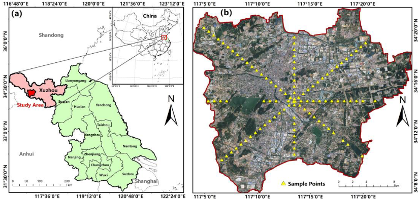
2.1. Study Area

The built-up area of Xuzhou City (Figure 1) was selected as the study area, which is located in the northwest of Jiangsu Province, China (between 116°22′–118°40′ E and 33°43′–34°58′ N). In this study, the built-up area refers to the highly urbanized areas dominated by artificial buildings and roads in the main urban area of Xuzhou (including Quanshan District, Gulou District, Yunlong District, Tongshan District, and Jiuli District). Approximately 90% of the area of Xuzhou is dominated by plains, with an average altitude of approximately 40 m. Xuzhou is also located in a typical warm temperate zone and semi monsoon region, with an annual average temperature of 14 °C and an annual average rainfall of 800–930 mm. By the end of 2021, the GDP of Xuzhou reached 127.32 billion USD, a permanent population of 9.0285 million, and an urbanization rate of 66.2%. From 1995 to 2019, Xuzhou experienced rapid urbanization, with the scale of the urban built-up area increasing from 59 km² to 274 km² [37]. Xuzhou is also an important transportation hub, coal-producing area, and power-base in eastern China. In addition, Xuzhou has a large-scale manufacturing industry. Rapid urbanization and industrialization have intensified the expansion of the IPS area and enhanced the UHI effect in the built-up areas of Xuzhou City. As a typical medium-sized city in China, Xuzhou has a high level of urbanization, industrialization, and transportation. It is not only widely distributed by impervious surfaces, but also has a significant UHI effect [20]. Therefore, the study area is very suitable for exploring the influence of IPS spatial characteristics on the heat island effect.

2.2. Data

Three scenes of Landsat 8 images from 2014 to 2020 were downloaded from the United States Geological Survey (USGS) data center (https://glovis.usgs.gov/, accessed on 1 September 2022). Their multispectral (bands 1–7) and thermal infrared (band 10) bands provide spatial source data for land surface component extraction and LST inversion, respectively. The time interval of the three images is 3 years. During these two periods, Xuzhou City was in the process of rapid urbanization, and the IPS has experienced obvious evolution, which is conducive to reflecting the effects of different IPS spatial patterns on LST. In addition, the three images are all in May (close to summer), which can not only show a significant UHI effect, but also avoid the impact of seasonal differences on the research results. Another satellite dataset used in pixel unmixing validation was the GF-1 high-resolution remote sensing image obtained in April 2020, whose spatial resolution reached 2 m with the fusion of panchromatic and multispectral bands. It should be noted that there was only a 19-day difference in the acquisition date of the GF-1 image and the corresponding Landsat 8 data in 2020. Therefore, the land cover change during this period can be ignored.

In addition, ground observations at the transit time of the Landsat 8 satellite, including near-surface temperature (T_air) and air relative humidity (RH), were also necessary for LST retrieval. The ground observations of May 1, 2014, and May 16, 2017, were collected from the Collaborative Observation Test Site of China University of Mining and Technology in the study area (data recording frequency of 30 min), and the meteorological data of May 17, 2020, were obtained from the NOAA National Centers for Environmental Information (NCEI) of USA (https://www.ngdc.noaa.gov/, accessed on 7 September 2022) (recording frequency of 1 h). All of the satellite data and ground observations are presented in

Table 1. Remote sensing data information and ground meteorological observation data.

Sensor Type	Image ID	Acquisition Time (GMT)	Air Temperature Tair (K)	Air Relative Humidity RH (%)
Landsat 8 OLI: 30 m TIRS: 100 m	LC81210362014121LGN00	1 May 2014 02:42:29	297.42	55.12
	LC81220362017136LGN00	16 May 2017 02:48:22	296.33	39.76
	LC81210362020138LGN00	17 May 2020 02:42:10	299.48	53.19
GF-1 PAN: 2 m MSS: 8 m	GF1_PMS1_E117.2_N34.1_20200428_L1A0004767917	28 April 2020 03:14:21 & 03:14:17
	GF1_PMS1_E117.3_N34.4_20200428_L1A0004767915

.

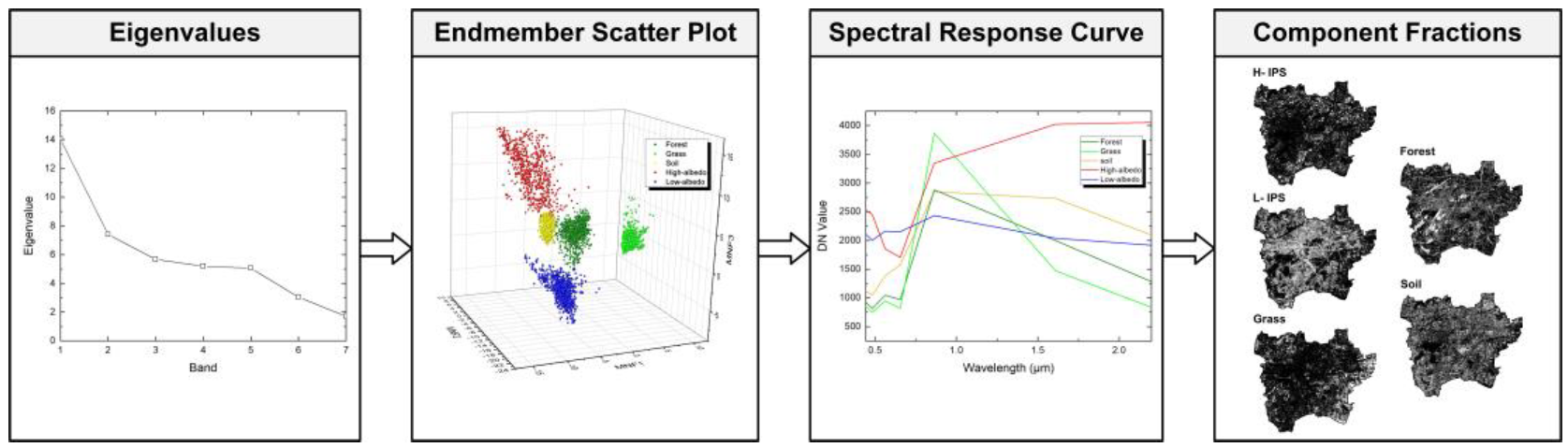
2.3. IPS Density Extraction from Mixed Pixels

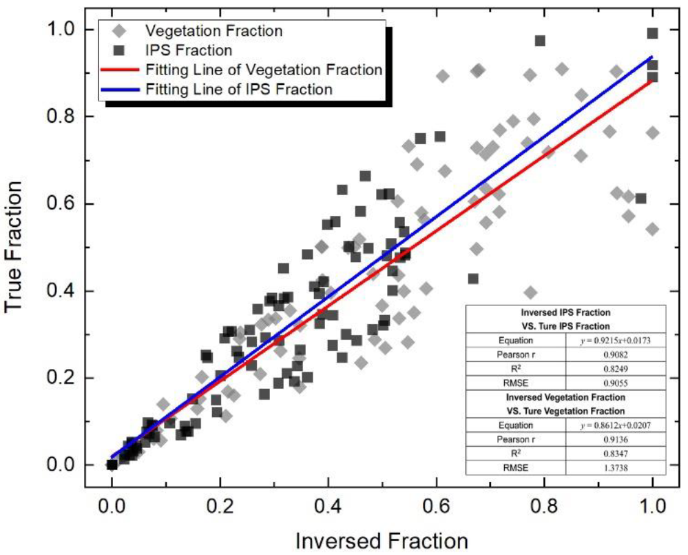
2.3.1. Endmember Fraction Extraction

Urban land cover can be expressed as a combination of three ecological elements (vegetation, impervious surface, and soil) at a certain ratio, using the vegetation-impervious surface-soil (V-I-S) model [36]. In medium- and low-resolution remote sensing images, a single pixel often contains more than two land cover components. The linear spectral mixture analysis (LSMA) model assumes that the reflectance of each mixed pixel in a certain band has a linear relationship with the reflectance of all components in the pixel, and the linear coefficient is the area proportion of each component [22]. Therefore, the least-squares method can be used to solve the component fractions of the mixed pixels. However, without any constraints, an endmember fraction extracted by the LSMA may be greater than 1 or less than 0, or the sum of all endmember fractions in a mixed pixel is not equal to 1. Then, the fully constrained linear spectral mixture analysis (FCLS) [38] was developed by considering the two constraints. On this basis, a normalized spectral mixture analysis model (NSMA) was proposed to further solve the negative impact of shadows on mixed pixel decomposition results [39]. Based on the diversity of impervious surfaces in the study area, the endmembers in a mixed pixel were divided into grass (including farmland), forest, soil, and high- and low-albedo impervious surfaces (water generally exists independently and can be masked). The LSMA algorithms are as follows.

$$\overline{R_b}=\frac{R_b}{\frac{1}{N}{{\displaystyle \sum }}_{b=1}^N\times R_b}\times 100$$

(1)

$$\overline{R_b}={\displaystyle \sum }_{i=1}^N{f}_i\overline{R_{i,b}}+e_b$$

(2)

$${\displaystyle \sum }_{i=1}^N{f}_i=1,f_i\ge 0$$

(3)

$$RMS={({\displaystyle \sum }_{b=1}^N{e}_b/N)}^{0.5}$$

(4)

where $\overline{R_b}$ is the standardized reflectance of a mixed pixel for band b; R_b is the original reflectance of the mixed pixel for band b; N is the endmember number of the mixed pixel; f_i is the fraction of endmember i; $\overline{R_{i,b}}$ is the standardized reflectance of endmember i for band b; e_b is the model calculation residual for band b; and RMS is the fitting accuracy of the LSMA model.

Sample selection of each endmember should be completed in ENVI 5.3 before LSMA, as shown in Figure 2. First, the eigenvalues of all bands were calculated using the minimum noise fraction rotation (MNF), which can be used to eliminate nonmajor bands. The pure pixels of all endmembers were extracted from the major bands of the MNF using the pure pixel index (PPI). Finally, the pure pixels were superposed onto the major bands of the MNF as a region of interest to generate a scatter plot in the ENVI n-D visualizer, and each clustered scatter cloud was marked as the sample of an endmember. After the endmember fractions were extracted using the NSMA model, the IPSD was calculated as the sum of the fractions of the high- and low-albedo IPS.

2.3.2. Endmember Fraction Validation

The endmember fractions extracted through the LSMA should be validated using high-resolution maps of land cover types. As shown in Figure 1b, all the sample points were set at intervals of 900 m along the four directions. Each pixel containing a sample point was regarded as the center pixel to create a 90 × 90 m² sample area. The fractions of IPS (including high- and low-albedo) and vegetation (including grass and forest) were then extracted from each sample area. All sample areas were superimposed on the GF-1 image, and manual interpretation was used to extract the proportions of land cover types in each sample area, which can be regarded as the true values of the component fractions. Although we have only found one phase of high-resolution satellite images whose transit time was close to the acquisition date of the Landsat 8 data of 2020, the pixel unmixing of the three Landsat 8 images was completely consistent with the rules and methods of endmember extraction. Therefore, the validation result of 17 May 2020 can represent the accuracy of the LSMA in this study.

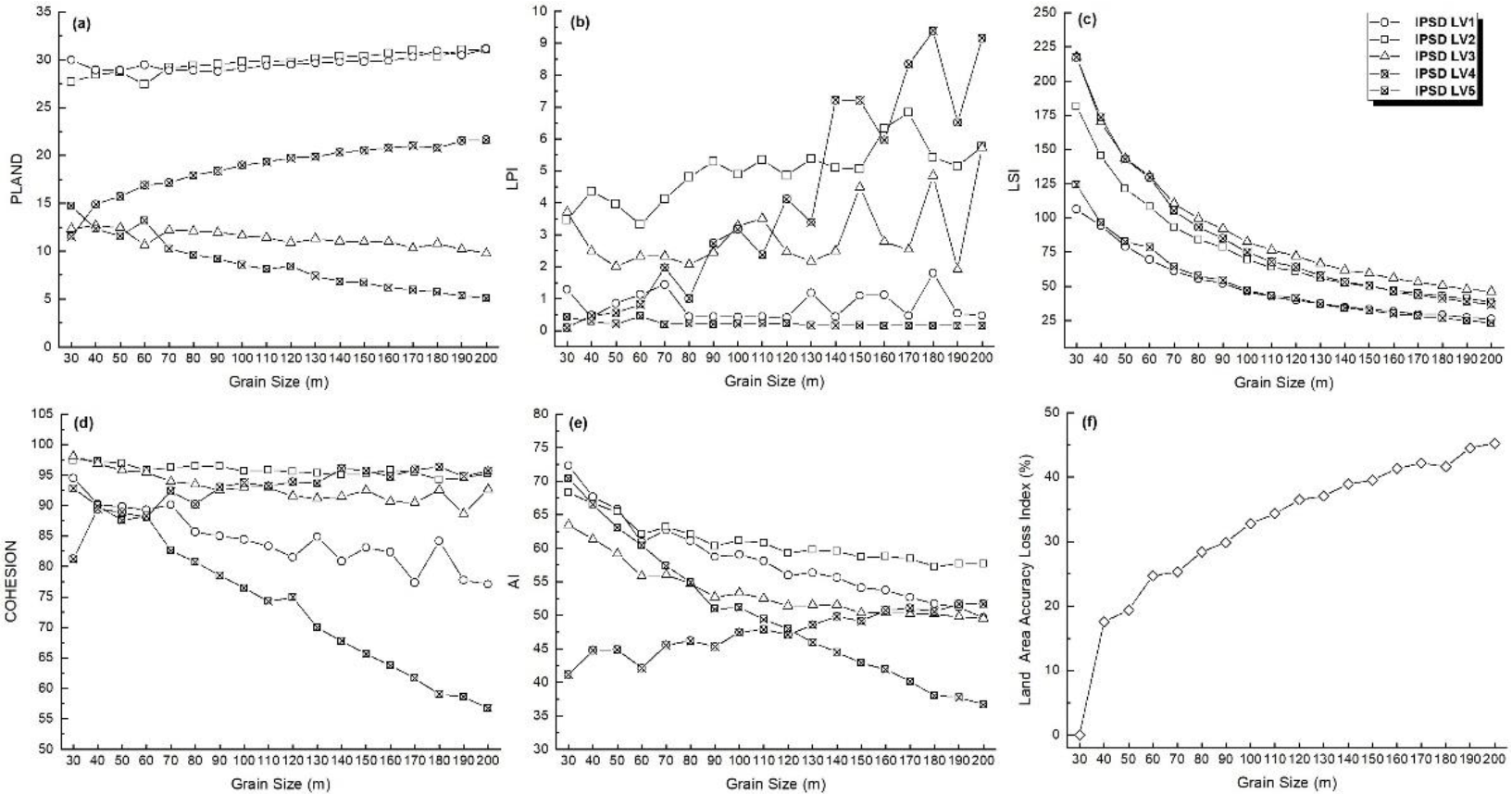
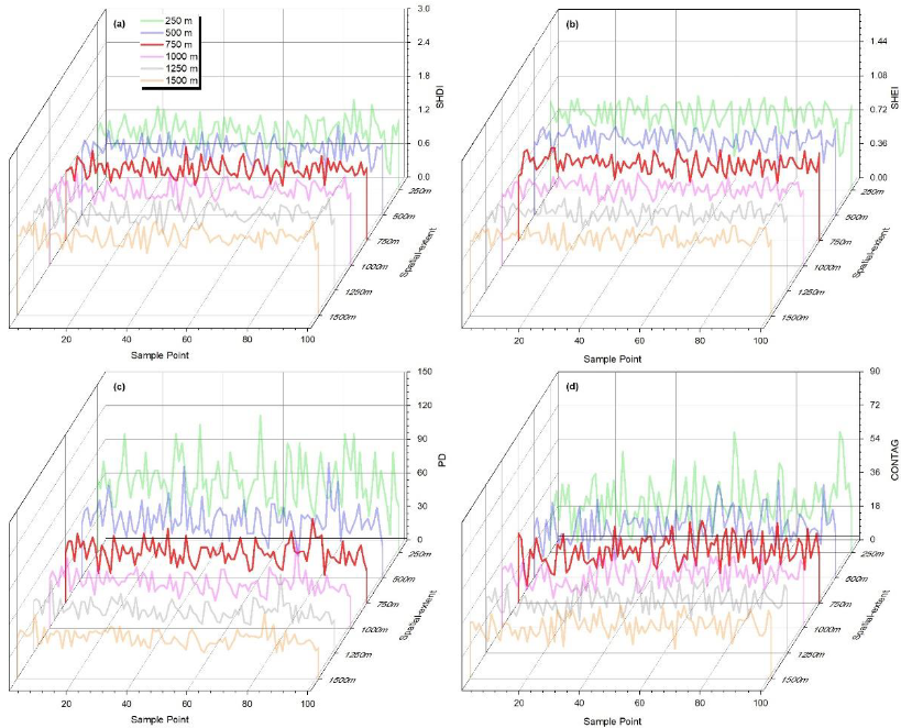
2.4. Landscape Pattern Analysis of IPS Density Levels

2.4.1. Landscape Metrics Selection for Five ISPD Levels

According to the IPSD values, the study area was classified into five levels using the mean-standard deviation method, including extremely high (LV5), sub high (LV4), medium (LV3), sub low (LV2), and low (LV1). The five levels were regarded as patches with various IPSDs to explore the effects of their landscape patterns on the UHI effect.

The proportion, shape complexity, predominance, natural connectivity, and aggregation are the five typical factors that can represent the spatial characteristics of patches, and the landscape metric is an effective approach for quantifying these spatial features [27]. Therefore, five class-level metrics–percentage of landscape (PLAND), landscape shape index (LSI), largest patch index (LPI), patch cohesion index (COHESION), and aggregation index (AI)–were selected to represent these spatial characteristics of each IPSD level, respectively. In addition, four landscape-level metrics: Shannon’s diversity index (SHDI), patch diversity (PD), Shannon’s evenness index (SHEI), and competition (CONTAG), were selected to represent the diversity, number, distribution, and aggregation of all IPSD levels in the same region. All of the selected landscape metrics are listed in

Table 2. The landscape metrics selected in this study.

Landscape Metrics		Formulas
Class level	PLAND	$\left({\displaystyle {\displaystyle \sum }_{j=1}^n}{a}_{ij}/A\right)\times 100$
	LPI	$\left[\max \left(a_{ij}\right)/A\right]\times 100$
	LSI	$e_i/min\left(e_i\right)$
	AI	$\left[\frac{g_{ii}}{max\to g_{ii}}\right]\times 100$
	COHESION	$\left\{1-\left[{\displaystyle {\displaystyle \sum }_{i=1}^m}{\displaystyle {\displaystyle \sum }_{k=1}^m}{p}_{ij}/{\displaystyle {\displaystyle \sum }_{i=1}^m}{\displaystyle {\displaystyle \sum }_{k=1}^m}\left(p_{ij}\times \sqrt{a_{ij}}\right)\right]\right\}\times {\left(1-1/\sqrt{Z}\right)}^{-1}\times 100$
Landscape level	SHDI	$-{\displaystyle {\displaystyle \sum }_{i=1}^n}\left[p_i\times ln\left(p_i\right)\right]$
	SHEI	$-{\displaystyle {\displaystyle \sum }_{i=1}^n}\left[p_i\times \ln \left(p_i\right)\right]/ln\left(m\right)$
	PD	$N/A$
	CONTAG	$\left\{1+\left[{\displaystyle {\displaystyle \sum }_{i=1}^m}{\displaystyle {\displaystyle \sum }_{k=1}^m}\left(p_i\times \frac{g_{ik}}{{{\displaystyle \sum }}_{j=1}^n{g}_{ij}}\right)\times \right.\right.\left.\left.ln\left(p_i\times g_{ik}/{\displaystyle {\displaystyle \sum }_{j=1}^n}{g}_{ij}\right)\right]/\left[2ln\left(m\right)\right]\right\}\times 100$

.

2.4.2. Scale Effect Analysis

In the assessment of landscape patterns and processes, most landscape metrics are highly dependent on the observation scale, particularly in remote sensing-based research, as the scale effect may affect the survey results of landscape structure [40]. The scale effect has two aspects: the grain-size effect and spatial-extent effect [41], which represent the impact of the variations of the size of the smallest spatial analysis unit and the analysis extent on landscape structure extraction, respectively. First, the best grain size should be analyzed. Each IPSD level map was resampled at 10 m interval from 30–200 m to produce 18 images with different spatial resolutions (grain-sizes). FRAGSTATS 4.2 was used to calculate the class-level metrics of these resized images, and the response trend of each metric to the change in grain-size was recorded, as shown in Figure 3a–e (taking the data of 17 May 2020 as an example). It can be seen that the inflection points of the response curves of most metrics occur at the position where the grain-size is 50 m. In addition, according to the land area information loss index (Figure 3f) calculated using Equations (5) and (6), the land area accuracy loss at a grain-size of 50 m is relatively low. Therefore, 50 m can be selected as the best grain-size for landscape pattern analysis of IPSD levels.

$$L_j=\left(A_j-A_{bj}\right)/A_{bj}\times 100$$

(5)

$$S_j=\sqrt{\frac{{{\displaystyle \sum }}_{j=1}^n{L}_j^2}{n}}$$

(6)

where L_j is the relative value of the patch area loss of IPSD level j, A_j is the patch area of IPSD level j at a converted grain size, A_bj is the patch area of IPSD level j at the original grain size, n is the number of IPSD levels, and S_j is the land area loss index.

The moving-window method was applied to calculate landscape metrics [42,43]. The landscape metrics within the spatial-extent of the moving-window window were assigned to the center pixel of the window and then moved to the next extent, and the spatial distribution map of each landscape metric was produced. The spatial-extent effect can be analyzed by adjusting the moving window size. To avoid pixel segmentation, the tested moving window sizes (spatial-extent) should be set as multiples of the best grain-size (n × 50 m). Therefore, six moving-window sizes at 250 m intervals from 250 × 250 m² to 1500 × 1500 m² were tested. FRAGSTATS 4.2 was applied to calculate the spatial distribution maps of four landscape-level metrics for six tested moving-window sizes, respectively. The sample points shown in Figure 1b were used to extract these metrics, as shown in Figure 4. The fluctuation curves of the four landscape-level metrics began to stabilize when the moving-window size increased to 750 × 750 m², which indicates that 750 × 750 m² can be set as the best spatial-extent for analyzing the landscape patterns of the IPSD levels.

2.5. Landscape Surface Temperature Retrieval

Landsat 8 has two thermal infrared bands, 10 and 11. Owing to the uncertainty of information in band 11 [23,24], band 10 was selected as the thermal radiation data. The mono-window algorithm [44,45] based on the thermal radiation transfer equation was used for LST inversion. The algorithm requires three parameters: land surface emissivity(ε), atmospheric transmittance (τ), and effective average atmospheric temperature (T_{air_e}). ε is determined by the thermal physical characteristics of the land cover types and is primarily affected by the atmospheric water vapor content (w), and T_{air_e} is related to atmospheric temperature and water vapor distribution. Previous research reported that the inversion accuracy of the mono-window algorithm was ±1.4 °C [45], and the equations were as follows:

$$LST=\left\{a\left(1-C-D\right)+\left[b\left(1-C-D\right)+C+D\right]T_{10}-D{T}_{air\_e}\right\}/C$$

(7)

$$C=\epsilon \tau$$

(8)

$$D=\left(1-\tau \right)\left[1+\left(1-\epsilon \right)\tau \right]$$

(9)

$$T_{10}=1321.08/ln\left(1+774.89/L_{10}\right)$$

(10)

$$\epsilon =P_v{R}_v{\epsilon }_v+\left(1-P_v\right)R_x{\epsilon }_x+d_{\epsilon }$$

(11)

where a = −62.7182 and b = 0.4339 are the regression coefficients of the Planck blackbody radiation function within 0–70 °C; T₁₀ is the brightness temperature calculated by thermal infrared band 10; L₁₀ is the thermal radiation parameter calculated by the DN value of band 10; P_v is the proportion of vegetation area to pixel, which can be calculated by the Normalized Difference Vegetation Index (NDVI); R_v and R_x (R_m or R_s) represent the radiation ratios of pure vegetation pixels, building pixels, and soil pixels, respectively; and d_ε is the interference value of the interaction between vegetation and soil on the land surface emissivity.

According to the simulation results of the Modern Resolution Atmospheric Transmission (MODTRAN 4) program, the linear relationships between τ and w for Landsat 8 TIR band 10 are shown in

Table 3. Regression functions for T_{air_e} and τ estimation.

w (g·cm−2)	τ Functions
0.2–1.6	0.9184–0.0725 w
1.6–4.4	1.0163–0.1330 w
4.4–5.4	0.7029–0.0620 w

[45]. Although the atmospheric water content data of the study area are not directly obtained, they can be calculated according to the empirical formula fitted from the historical data of the China Meteorological Station. The necessary parameters included the average altitude (H_E = 40 m), the latitude (φ = 34.24°), and the relative air humidity (RH) of the study area, as shown in Equations (12) and (13) [46]. In the mid-latitude summer, the linear relationship between T_{air_e} and T_air is shown in Equation (14) [44].

$$w=0.03exp\left(-1.39H_E{}^2+2.74H_E+0.15\right)e+\frac{0.066}{{\left(\phi -33\right)}^2+4.41}+0.17$$

(12)

$$e=0.6112exp(\frac{17.67T_{air}}{T_{air}+243.5})\times RH$$

(13)

$$T_{air\_e}=16.0110+0.9262T_{air}$$

(14)

2.6. Bivariate Moran’s I Analysis

Two types of bivariate Moran’s I [47] were applied to explore the spatial correlation between landscape metrics of IPSD levels and LST, namely bivariate global Moran’s I and bivariate local Moran’s I. Bivariate global Moran’s I indicated whether there is spatial correlation between landscape metrics and LST in the whole region and the degree of their spatial correlation, while bivariate local Moran’s I shows the spatial correlations in different spatial units. The equations are as follows:

$$I=\frac{{{\displaystyle \sum }}_{i=1}^n{{\displaystyle \sum }}_{j=1}^n{W}_{ij}\left(x_i-\overline{x}\right)\left(y_j-\overline{y}\right)}{S^2{{\displaystyle \sum }}_i^n{{\displaystyle \sum }}_{j=1}^n{W}_{ij}}$$

(15)

$$I_i=Z_i{{\displaystyle \sum }}_{j=1}^n{W}_{ij}{Z}_j$$

(16)

where I and I_i are the bivariate global and local spatial autocorrelation indices, respectively; n is the total number of spatial units; W_ij is the spatial weight matrix established by K adjacency method; x_i and y_j are the observed values of independent variable and dependent variable in spatial unit i and j respectively; S² is the variance of all samples; z_i and z_j are the normalized values of the variances of the observations in spatial units i and j.

The values of I and I_i range from −1 to 1. A positive value indicates a positive spatial correlation between landscape metrics and LST, meaning that pixels with high landscape metric values may be surrounded by pixels with high LST values. By contrast, a negative value represents a negative spatial correlation, indicating that pixels with high landscape metric values may be surrounded by pixels with low LST values. The larger the absolute values of I and I_i, the stronger the spatial correlation between landscape metrics and LST. The four quadrants generated based on the local indicators of spatial association (LISA) of I_i represent four types of local spatial autocorrelation [48]. Quadrant I, called High–High (HH) type, represents the high landscape metrics value surrounded by high LST value; Quadrant II is High–Low (HL), indicating the high landscape metrics value surrounded by low LST value; Quadrant III is Low–Hight (LH), indicating a low landscape metrics value surrounded by a high LST value; and Quadrant IV is Low–Low (LL), indicating the low landscape metrics value surrounded by low LST values.

3. Results

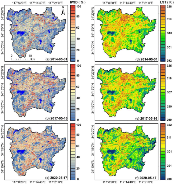
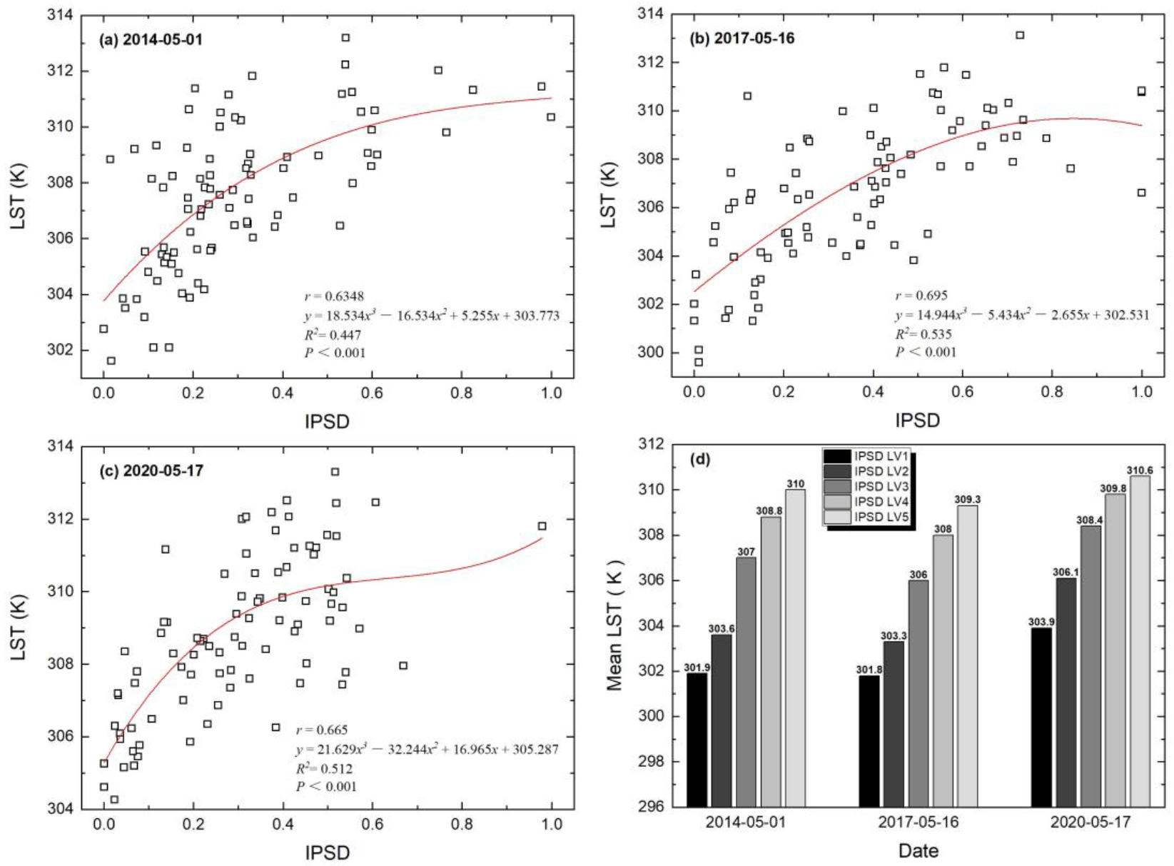
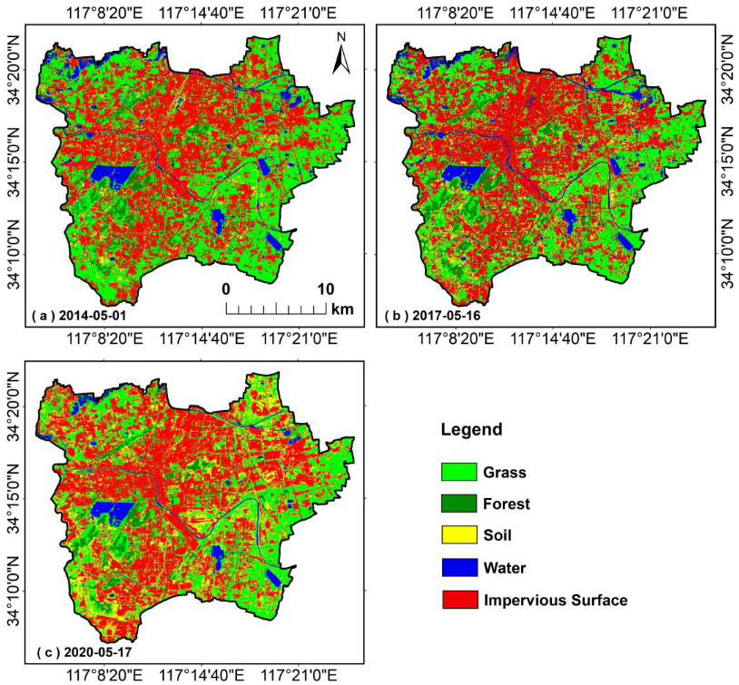
3.1. Inversion Results of IPSD and LST

The IPSD maps calculated by LSMA are shown in Figure 5a–c. Compared with the high-resolution land cover data extracted from the GF-1 image (Figure 6), the inversed fractions (taking the components of IPS and vegetation on 17 May 2020, as an example) had a significant and strong linear correlation with the true fractions (with r > 0.90 and R² > 0.82, p < 0.001), which signified that the accuracy of the inversed IPSD was reliable. The IPS area of the study area has gradually expanded, and high-density impervious patches have significantly increased, which is consistent with the rapid urbanization of Xuzhou City during this period. The LST images retrieved by the mono-window algorithm are shown in Figure 5d–f. From 2014 to 2020, the study area also showed an apparent UHI effect, and the LST of the areas covered by IPS was higher than that of the surrounding vegetation, soil, and other natural surfaces. IPSD and LST values were extracted by the sample points shown in Figure 1b. The quantitative relationship between IPSD and LST is simulated using linear, quantitative, cubic and empirical regression models, respectively. The results are shown in

Table 4. Regression results between IPSD and LST by applying four models.

Date	Regression Model	R2	F	Siginficance
1 May 2014	Linear	0.403	56.692	0.000
	Quadratic	0.446	33.364	0.000
	Cubic	0.447	22.080	0.000
	Exponential	0.402	56.571	0.000
16 May 2017	Linear	0.482	78.297	0.000
	Quadratic	0.534	47.616	0.000
	Cubic	0.535	31.403	0.000
	Exponential	0.482	78.295	0.000
17 May 2020	Linear	0.443	66.734	0.000
	Quadratic	0.489	41.132	0.000
	Cubic	0.512	28.699	0.000
	Exponential	0.443	66.894	0.000

. It can be seen that the fitting results of the four regression models are significant at p < 0.001, and the cubic model has the highest fitting goodness (with 0.447 < R² < 0.535) for three phases. Figure 7a–c reveals that the LST of three phases generally shows an upward trend with the increase of IPSD, with Pearson’s correlation coefficients of 0.63, 0.69, and 0.66, respectively. In addition, as shown in Figure 7d, the average LST of each IPSD level indicated that the average LST also increased with an increase in the IPSD level, which further proved the enhancement effect of IPSD on the thermal environment. Therefore, it is valuable to further explore the spatial relationship between landscape patterns of IPSD levels and LST.

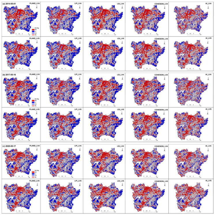
3.2. Spatial Correlation between Landscape Metrics of IPSD Levels and LST

The bivariate global Moran’s I values between landscape metrics of the five IPSD levels and LST are listed in

Table 5. Bivariate Global Moran’s I between landscape metrics of IPSD levels and LST.

Landscape Metrics of IPSD Levels	1 May 2014		16 May 2017		17 May 2020
	Moran’s I	z-Value	Moran’s I	z-Value	Moran’s I	z-Value
PLAND_LV1	−0.4104 ***	−484.3881	−0.3640 ***	−445.4438	−0.5860 ***	−624.7005
PLAND_LV2	−0.6232 ***	−685.0685	−0.575	−650.749	−0.5059 ***	−570.771
PLAND_LV3	0.1072 ***	137.3938	0.0677 ***	87.2685	0.1210 ***	151.1338
PLAND_LV4	0.5383 ***	614.4767	0.5590 ***	643.6663	0.5756 ***	631.9944
PLAND_LV5	0.5694 ***	620.9965	0.6040 ***	676.2391	0.5970 ***	644.6729
LPI_LV1	−0.3197 ***	−393.3837	−0.3121 ***	−389.215	−0.5315 ***	−583.4593
LPI_LV2	−0.5868 ***	−654.7533	−0.5346	−614.5225	−0.4395 ***	−505.6169
LPI_LV3	0.0647 ***	81.7962	0.0180 ***	23.9672	0.0641 ***	82.5256
LPI_LV4	0.4297 ***	488.2168	0.3920 ***	478.9052	0.4547 ***	523.3753
LPI_LV5	0.4673 ***	559.9899	0.5190 ***	585.9848	0.4871 ***	544.9192
LSI_LV1	−0.4573 ***	−532.3214	−0.3848 ***	−461.4945	−0.4999 ***	−563.362
LSI_LV2	−0.4002 ***	−476.3153	−0.3055 ***	−392.9659	−0.4857 ***	−540.3122
LSI_LV3	0.1536 ***	195.9282	0.1254 ***	158.7598	0.1820 ***	220.0359
LSI_LV4	0.5388 ***	606.2473	0.5350 ***	626.5211	0.5551 ***	609.7773
LSI_LV5	0.5870 ***	648.4811	0.5832 ***	656.4933	0.5881 ***	636.8686
COHESION_LV1	−0.3765 ***	−448.9476	−0.3388 ***	−412.4622	−0.5433 ***	−599.7174
COHESION_LV2	−0.5047 ***	−576.0259	−0.4572 ***	−529.8952	−0.4486 ***	−522.592
COHESION_LV3	0.0579 ***	73.9933	0.0410 ***	53.2148	0.0860 ***	113.1896
COHESION_LV4	0.4797 ***	537.8656	0.4602 ***	542.6128	0.5117 ***	564.794
COHESION_LV5	0.4883 ***	578.6784	0.5277 ***	597.2353	0.5227 ***	579.8648
AI_LV1	−0.2701 ***	−331.9032	−0.2186 ***	−275.91	−0.4366 ***	−511.5759
AI _LV2	−0.4040 ***	−474.7578	−0.3443 ***	−421.8647	−0.2690 ***	−329.8153
AI _LV3	0.0114 ***	14.3478	0.0210 ***	27.7116	0.0382 ***	49.9856
AI _LV4	0.2148 ***	256.5564	0.2014 ***	254.5295	0.2943 ***	340.0671
AI _LV5	0.3271 ***	411.6849	0.3711 ***	444.3869	0.3693 ***	437.643
SHDI	0.0444 ***	57.7489	0.1342 ***	176.6873	0.0123 ***	15.8512
SHEI	0.2120 ***	275.7464	0.2885 ***	366.9209	0.1894 ***	240.8287
PD	0.1598 ***	203.1749	0.1885 ***	248.4368	0.1525 ***	192.6977
CONTAG	−0.2891 ***	−366.797	−0.3494 ***	−432.5666	−0.2885 ***	−356.5613

*** Statistically significant p < 0.001.

Significant spatial correlations were observed between all the selected landscape metrics and LST. However, these spatial correlations show great differences with variations in landscape metrics and IPSD levels. For landscape-level metrics, SHDI, SHEI, and PD showed significant positive spatial correlations with LST (p < 0.001), indicating that increasing the number of IPSD levels, patch even distribution degree, and patch density could enhance the regional thermal environment. In contrast, CONTAG showed a significant negative spatial correlation with LST (p < 0.001), which signified that increasing the aggregation degree of the five IPSD levels would alleviate the UHI effect.

For class-level metrics which represent the independent spatial characteristics of the patches of each IPSD level for an area, PLAND, LPI, LSI, AI, and COHESION showed significant correlations (p < 0.001) with LST, indicating that the spatial characteristics of each IPSD level, such as patch proportion, predominance degree, shape complexity, aggregation degree, and natural connectivity degree, have significant spatial impacts on the thermal environment. However, the direction and degree of these spatial impacts varied at different IPSD levels. First, the bivariate global Moran’s I between LST and class-level metrics of IPSD LV1 or LV2 were negative. Second, the bivariate global Moran’s I between LST and class-level metrics of IPSD LV3 to LV5 were positive, and the value of Moran’s I increased gradually as the level of IPSD increased.

In addition, LST have an obviously stronger spatial correlation with the class-level metrics of IPSD LV4 and LV5 (0.2 < Moran’s I < 0.6) than IPSD LV3 (most Moran’s I < 0.1). Therefore, the class-level metrics of IPSD LV4 and LV5 are key factors that affect the spatial characteristics of the thermal environment and deserve special attention. Based on the degree of spatial correlation between the LST and class-level metrics of IPSD LV4 or LV5, these metrics can be sorted as PLAND (average Moran’s I = 0.57), LSI (average Moran’s I = 0.56), COHESION (average Moran’s I = 0.50), LPI (average Moran’s I = 0.46), and AI (average Moran’s I = 0.30). However, the spatial correlation degree cannot fully represent the contribution ratio of each class-level metric of IPSD LV4 and LV5 to LST; therefore, further discussion on the impact weights of these metrics is necessary.

The bivariate local Moran’s I between the class-level metrics of IPSD LV4 or LV5 and LST are represented as LISA maps (Figure 8), which show the spatial distributions of the correlation between the two variables. The spatial clustering mode between the class-level metrics (PLAND, LSI, COHESION, LPI, and AI) and LST were mostly HH and LL. The superposition results of LISA maps and land cover classification maps (Figure A1 in Appendix A) showed that most of the HH areas were distributed in urban built-up areas with IPS coverage, whereas LL areas were mainly distributed in urban forests and parks with vegetation coverage, as well as farmland in the suburbs.

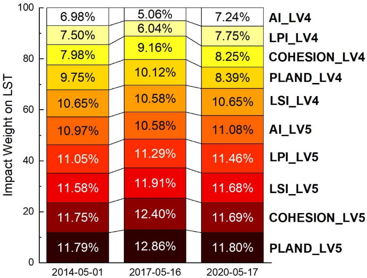
3.3. The Impact Weights of Class-Level Metrics of IPSD LV4 and LV5 on LST

The spatial correlation analysis in the previous sections proved that class-level metrics of IPSD LV4 and LV5 have significant negative spatial effects on LST. However, the contribution of each metric to the spatial impact on LST still needs to be discussed further. In general, the standardized coefficients of multiple linear regression (MRA) can be used to express the contribution weight of each independent variable (class-level metrics of IPSD LV4 and LV5) to the dependent variable (LST). However, the multicollinearity among these metrics was revealed during testing, which prevented the direct use of MRA. The principal component analysis (PCA) can recombine multiple original highly correlated independent variables into a group of unrelated comprehensive variables, which are called major component variables (F_i) [49]. As collinearity was eliminated among the principal component variables, MRA could be directly used to extract standardized regression coefficients (β_i) between F_i and LST. Finally, the impact weights of each class-level metric of IPSD LV4 and LV5 on LST were calculated using the eigenvalue (η_i) of the major component variables, the PCA component matrix, and the standardized regression coefficients.

All independent and dependent variables were standardized before PCA. The total variance explained by PCA (

Table 6. Total variance explained by principal component analysis.

Date	KMO	Sums of Squared Loadings	F1 ①	F2 ①
1 May 2014	0.7596	Eigenvalue (ηi)	4.076	3.836
		Cumulative Percent (%)	79.119
16 May 2017	0.7335	Eigenvalue (ηi)	3.942	3.928
		Cumulative Percent (%)	78.706
17 May 2020	0.7387	Eigenvalue (ηi)	4.030	3.868
		Cumulative Percent (%)	78.985

^① F₁ and F₂ are components 1 and 2 extracted through PCA, respectively.

) showed that the Kaiser–Meyer–Olkin measure of sampling adequacy (KMO) values were all above 0.73, indicating that the PCA method was applicable to the independent variables of the class-level metrics of IPSD LV4 and LV5. Two principal components (F₁ and F₂) were extracted from the independent variables of the three phases, and all cumulative proportions of variance were more than 78%, indicating that F₁ and F₂ could effectively represent all independent variables.

The component matrix of PCA represents the correlation coefficient (θ₁ and θ₂) of all the original independent variables (V1 to V10) with each principal component variable (F₁ and F₂), which are shown in

Table 7. Component matrix of principal component analysis (PCA) ^①.

Normalized Original Variables (Class-Level VFLM)	1 May 2014		16 May 2017		17 May 2020
	F1 (θ1)	F2 (θ2)	F1 (θ1)	F2 (θ1)	F1 (θ1)	F2 (θ2)
(V1) PLAND_LV5	0.449	0.836	0.886	0.240	0.722	0.525
(V2) PLAND_LV4	0.209	0.855	0.902	0.278	/	0.882
(V3) LSI_LV5	0.624	0.635	0.835	/	0.877	0.358
(V4) LSI_LV4	0.871	0.282	0.623	0.630	0.233	0.888
(V5) LPI _LV5	0.897	0.300	0.873	/	0.320	0.888
(V6) LPI_LV4	0.809	/	0.522	0.719	/	0.815
(V7) COHESION_LV5	0.619	0.659	/	0.874	0.635	0.599
(V8) COHESION_LV4	0.861	/	0.240	0.905	0.874	/
(V9) AI _LV5	0.304	0.893	/	0.732	0.901	0.270
(V10) AI_LV4	/	0.764	0.377	0.870	0.767	/

^① Rotation Method: Varimax with Kaiser Normalization.

(where θ_i < 0.2 was considered to be too low and was rejected). As shown in Equations (18) and (19) [49], F₁ and F₂ can be calculated as the weighted sum of the original variables and their contribution coefficient α_ij (calculated using Equation (17)).

$${\alpha }_{ij}=\frac{{\theta }_{ij}}{\sqrt{{\eta }_i}}$$

(17)

$$F_1={\alpha }_{11}V1+{\alpha }_{12}V2+{\alpha }_{13}V3+{\alpha }_{14}V4+{\alpha }_{15}V5+{\alpha }_{16}V6+{\alpha }_{17}V7+{\alpha }_{18}V8+{\alpha }_{19}V9+{\alpha }_{110}V10$$

(18)

$$F_2={\alpha }_{21}V1+{\alpha }_{22}V2+{\alpha }_{23}V3+{\alpha }_{24}V4+{\alpha }_{25}V5+{\alpha }_{26}V6+{\alpha }_{27}V7+{\alpha }_{28}V8+{\alpha }_{29}V9+{\alpha }_{210}V10$$

(19)

Table 8. Multiple linear regression coefficients between normalized LST and principal variables (F₁ and F₂).

Regression Coefficients		1 May 2014	16 May 2017	17 May 2020
r		0.599 ***	0.640 ***	0.650 ***
R2		0.359 ***	0.410 ***	0.422 ***
Standardized Coefficients (βi)	F1	0.317 ***	0.430 ***	0.345 ***
	F2	0.303 ***	0.245 ***	0.340 ***

*** Significant at p < 0.001

presents the multivariate linear regression results between the dependent variable normalized LST and independent variables F₁ and F₂. The significant and strong linear relationship between independent variables and dependent variables for each phase is evident ((with p < 0.001 and r > 0.59). Here, the impact weights (β_i) of F₁ and F₂ on the LST were obtained. Then, by combining β_i with the contribution coefficient α_ij of the original variables to F₁ and F₂, the impact weights of the class-level metrics of IPSD LV4 and LV5 on LST were calculated using Equation (20). Figure 9 shows that the impact weights of the class-level metrics of IPSD LV5 are higher than those of LV4. For the LV5 patches, the impact weights of the metrics were ranked from high to low as PLAND, COHESION, LSI, LPI, and AI. In addition, the impact weights of the first four metrics were similar, indicating that the spatial characteristics of IPSD LV5, such as area proportion, natural connectivity, shape complexity, and predominance degree have similar regulatory effects on the thermal environment. For the LV4 patches, the impact weights of the class-level metrics on LST were ranked differently from those of LV5, that is, LSI, PLAND, COHESION, LPI, and AI from high to low.

$$W_j={\alpha }_{1j}\times {\beta }_1+{\alpha }_{2j}\times {\beta }_2$$

(20)

4. Discussion

In recent studies on the relationship between the IPS spatial pattern and UHI, IPS is generally regarded as a single land cover type (such as a building or built-up area) in the calculation of landscape pattern metrics [8,49], without considering the impact caused by the difference of IPS density in the patches. Since the positive correlation between IPS and UHI has been proved by many studies [21,27], our study explored an innovative method to incorporate IPS density into landscape pattern analysis. According to the component fraction value of IPS, the land surface of the study area is classified into five levels (or can be regarded as five patch types), which corresponds to the land cover types in general landscape pattern analysis. Although the density index used for simple classification cannot completely simulate the urban IPS with high heterogeneous, it is still helpful to reveal the impact of the spatial pattern of the patches with various IPS densities on UHI.

It should be noted that landscape-level metrics represent the comprehensive spatial characteristics of the patches of all spatial elements in an area. The patches of the five IPSD levels have different ratios of natural surface and impervious surface (for example, level 1 contains higher natural surface and lower IPS ratios, while level 5 has the opposite ratios). Therefore, landscape-level metrics can be regarded as comprehensive spatial pattern indicators of vegetation and IPS patches with various proportions. This further indicates that the relationship between landscape-level metrics and LST results from the interaction between the IPS and natural patches in the region, including the enhancement effect of high IPS density patches (LV4 and LV5) on thermal environment and the mitigation effect of low IPS density patches (LV1 and LV2 with higher vegetation or soil density) on UHI.

In previous studies, IPS is generally regarded as one of the land cover types, and its class-level metrics PLAND, LPI, LSI, COHESION, and AI have been proved to have significant positive correlations with LST [50,51]. This is consistent with our results that these class-level metrics of IPSD LV3 to LV5 (with higher IPS proportion) show positive bivariate global Moran’s I with LST (p < 0.001).

From IPSD LV1 to LV2, the spatial patterns of the patches are negatively correlated with LST, which because these patches are mainly covered by natural surfaces (vegetation and soil) with low IPS proportions, resulting in that the mitigation effect of vegetation on the thermal environment is dominant. On the contrary, from IPSD LV3 to LV5, the spatial patterns of the patches began to be positively correlated with LST, which owing to the increase in IPSD is accompanied by the enhancement of surface thermal radiation and anthropogenic heat emissions, and the heating effect of IPS thermal completely offsets the cooling effect of natural surfaces. With the gradual increase of IPS density, Moran’s I tends to increase. In addition, the land cover type in IPSD LV5 patches are mostly IPS. However, IPSD LV4 patches are still mixed with more natural surfaces. This is an important reason for the difference in the impact weight rankings between the class-level metrics of LV4 and LV5. Previous research found that the landscape metric PLAND of building or built-up patches has the strongest correlation with LST [8], and the correlation between LPI and LST is stronger than that between AI and LST [51], which are also the same as our results. According to our research, priority should be given to reducing the area proportion, natural connectivity degree and shape complexity degree of high-density IPS regions, which could be one of the effective approaches to alleviate the regional thermal environment.

5. Conclusions

Based on three Landsat 8 images of the study area from 2014 to 2020, the LSMA and mono-window algorithms were used to extract the IPSD and LST, respectively. Landscape and geospatial analyses were applied to explore the spatial correlation between the landscape metrics of various IPSD levels and LST. It was revealed that the four landscape-level metrics, SHDI, SHEI, and PD all showed significant positive spatial correlations with LST, while CONTAG showed a significant negative correlation, indicating that increasing the regional number of IPSD levels, patch even distribution degree, and patch density, or reducing the aggregation degree between the five IPSD levels will lead to the enhancement of the thermal environment. It should be noted that the relationships between landscape-level metrics and LST reflect the comprehensive spatial effects of all IPSD level patches, which means that natural patches (mainly covered vegetation and soil) also contribute to these spatial effects on LST. For the five class-level metrics of each IPSD level, PLAND, LPI, LSI, AI, and COHESION, all showed significant correlations with LST. This means that the spatial characteristics of each IPSD level, such as patch proportion, predominance degree, shape complexity, aggregation degree, and natural connectivity degree, were all regulatory factors for the UHI effect. In particular, the degree of positive spatial correlation of the class-level metrics of IPSD LV4 and LV5 with LST were the highest. The impact weight of each class-level metric of IPSD LV4 and LV5 on LST was also obtained using PCA and MRA standardization coefficients, which can be sorted as PLAND_LV5 > COHESION_LV5 > LSI_LV5 > LPI_LV5 > AI_LV5 > LSI_LV4 > PLAND_LV4 > COHESION_LV4 > LPI_LV4 > AI_LV4. This study has revealed the importance of and differences in the spatial patterns of patches with various IPSDs in UHI effect regulation. It is suggested that in urban planning and environmental management, approaches to reduce the area proportion, natural connectivity degree, and shape complexity of regional high-density IPS are preferred to alleviate the UHI effect.

Considering the size, geographical location and industrial structure of the study area in this paper, our conclusions may be limited with regard to the applicability to medium-sized cities dominated by industry in central China. For other city types, such as agriculture-dominated cities, commerce-dominated cities, and super large cities, the impact of IPS spatial pattern on the UHI effect needs to be discussed further. In addition, owing to the fact that the transit time of Landsat 8 images are basically fixed, the inversion time of UHI effect in this paper is limited to noon (around 11:00 AM, Beijing time), which cannot further reveal whether the impact of the IPS’s spatial pattern on UHI varies with time. Another issue worth detailed study is the use of unmanned aerial vehicles (UAV) equipped with multispectral and thermal infrared sensors to obtain urban LST data at different times in one day, and to explore the temporal characteristics of the impact of IPS spatial patterns on the UHI effect.

References

1. Yan, Z.; Zhou, D.; Li, Y.; Zhang, L. An Integrated Assessment on the Warming Effects of Urbanization and Agriculture in Highly Developed Urban Agglomerations of China. Sci. Total Environ. 2022, 804, 150119. [Google Scholar] [CrossRef] [PubMed]
2. Ahmed, H.A.; Singh, S.K.; Kumar, M.; Maina, M.S.; Dzwairo, R.; Lal, D. Impact of Urbanization and Land Cover Change on Urban Climate: Case Study of Nigeria. Urban Clim. 2020, 32, 100600. [Google Scholar] [CrossRef]
3. Estoque, R.C.; Murayama, Y. Quantifying Landscape Pattern and Ecosystem Service Value Changes in Four Rapidly Urbanizing Hill Stations of Southeast Asia. Landsc. Ecol. 2016, 31, 1481–1507. [Google Scholar] [CrossRef]
4. Chao, Z.; van Dijk, A.I.J.M.; Wang, L.; Che, M.; Hou, S. Effects of Different Urbanization Levels on Land Surface Temperature Change: Taking Tokyo and Shanghai for Example. Remote Sens. 2020, 12, 2022. [Google Scholar] [CrossRef]
5. Santamouris, M. Recent Progress on Urban Overheating and Heat Island Research. Integrated Assessment of the Energy, Environmental, Vulnerability and Health Impact. Synergies with the Global Climate Change. Energy Build. 2020, 207, 109482. [Google Scholar] [CrossRef]
6. Da Silva, J.M.C.; Prasad, S.; Diniz-Filho, J.A.F. The Impact of Deforestation, Urbanization, Public Investments, and Agriculture on Human Welfare in the Brazilian Amazonia. Land Use Policy 2017, 65, 135–142. [Google Scholar] [CrossRef]
7. Yao, R.; Cao, J.; Wang, L.; Zhang, W.; Wu, X. Urbanization Effects on Vegetation Cover in Major African Cities during 2001–2017. Int. J. Appl. Earth Obs. Geoinf. 2019, 75, 44–53. [Google Scholar] [CrossRef]
8. Qin, L.; Liu, H.; Shang, G.; Yang, H.; Yan, H. Thermal Environment Effects of Built-Up Land Expansion in Shijiazhuang. Land 2022, 11, 968. [Google Scholar] [CrossRef]
9. Oke, T.R. The Energetic Basis of the Urban Heat Island. Q. J. R. Meteorol. Soc. 1982, 108, 1–24. [Google Scholar] [CrossRef]
10. Oke, T.R. The Distinction between Canopy and Boundary-Layer Urban Heat Islands. Atmosphere 1976, 14, 268–277. [Google Scholar] [CrossRef]
11. Estoque, R.C.; Murayama, Y. Monitoring Surface Urban Heat Island Formation in a Tropical Mountain City Using Landsat Data (1987–2015). ISPRS J. Photogramm. Remote Sens. 2017, 133, 18–29. [Google Scholar] [CrossRef]
12. Liu, K.; Li, X.; Wang, S.; Gao, X. Assessing the Effects of Urban Green Landscape on Urban Thermal Environment Dynamic in a Semiarid City by Integrated Use of Airborne Data, Satellite Imagery and Land Surface Model. Int. J. Appl. Earth Obs. Geoinf. 2022, 107, 102674. [Google Scholar] [CrossRef]
13. Jacob, D.J.; Winner, D.A. Effect of Climate Change on Air Quality. Atmos. Environ. 2009, 43, 51–63. [Google Scholar] [CrossRef] [Green Version]
14. Zhou, W.; Cao, F. Effects of Changing Spatial Extent on the Relationship between Urban Forest Patterns and Land Surface Temperature. Ecol. Indic. 2020, 109, 105778. [Google Scholar] [CrossRef]
15. Santamouris, M.; Cartalis, C.; Synnefa, A.; Kolokotsa, D. On the Impact of Urban Heat Island and Global Warming on the Power Demand and Electricity Consumption of Buildings—A Review. Energy Build. 2015, 98, 119–124. [Google Scholar] [CrossRef]
16. Zhou, W.; Huang, G.; Cadenasso, M.L. Does Spatial Configuration Matter? Understanding the Effects of Land Cover Pattern on Land Surface Temperature in Urban Landscapes. Landsc. Urban Plan. 2011, 102, 54–63. [Google Scholar] [CrossRef]
17. Wang, Y.; Du, H.; Xu, Y.; Lu, D.; Wang, X.; Guo, Z. Temporal and Spatial Variation Relationship and Influence Factors on Surface Urban Heat Island and Ozone Pollution in the Yangtze River Delta, China. Sci. Total Environ. 2018, 631–632, 921–933. [Google Scholar] [CrossRef]
18. Patz, J.A.; Campbell-Lendrum, D.; Holloway, T.; Foley, J.A. Impact of Regional Climate Change on Human Health. Nature 2005, 438, 310–317. [Google Scholar] [CrossRef]
19. Ma, X.; Peng, S. Research on the Spatiotemporal Coupling Relationships between Land Use/Land Cover Compositions or Patterns and the Surface Urban Heat Island Effect. Environ. Sci. Pollut. Res. 2022, 29, 39723–39742. [Google Scholar] [CrossRef]
20. Wang, Y.; Zhang, Y.; Ding, N.; Qin, K.; Yang, X. Simulating the Impact of Urban Surface Evapotranspiration on the Urban Heat Island Effect Using the Modified RS-PM Model: A Case Study of Xuzhou, China. Remote Sens. 2020, 12, 578. [Google Scholar] [CrossRef]
21. Song, J.; Chen, W.; Zhang, J.; Huang, K.; Hou, B.; Prishchepov, A.V. Effects of Building Density on Land Surface Temperature in China: Spatial Patterns and Determinants. Landsc. Urban Plan. 2020, 198, 103794. [Google Scholar] [CrossRef]
22. Li, L.; Canters, F.; Solana, C.; Ma, W.; Chen, L.; Kervyn, M. Discriminating Lava Flows of Different Age within Nyamuragira’s Volcanic Field Using Spectral Mixture Analysis. Int. J. Appl. Earth Obs. Geoinf. 2015, 40, 1–10. [Google Scholar] [CrossRef] [Green Version]
23. Barsi, J.; Schott, J.; Hook, S.; Raqueno, N.; Markham, B.; Radocinski, R. Landsat-8 Thermal Infrared Sensor (TIRS) Vicarious Radiometric Calibration. Remote Sens. 2014, 6, 11607–11626. [Google Scholar] [CrossRef] [Green Version]
24. Montanaro, M.; Lunsford, A.; Tesfaye, Z.; Wenny, B.; Reuter, D. Radiometric Calibration Methodology of the Landsat 8 Thermal Infrared Sensor. Remote Sens. 2014, 6, 8803–8821. [Google Scholar] [CrossRef] [Green Version]
25. Yuan, F.; Bauer, M.E. Comparison of Impervious Surface Area and Normalized Difference Vegetation Index as Indicators of Surface Urban Heat Island Effects in Landsat Imagery. Remote Sens. Environ. 2007, 106, 375–386. [Google Scholar] [CrossRef]
26. Du, H.; Wang, D.; Wang, Y.; Zhao, X.; Qin, F.; Jiang, H.; Cai, Y. Influences of Land Cover Types, Meteorological Conditions, Anthropogenic Heat and Urban Area on Surface Urban Heat Island in the Yangtze River Delta Urban Agglomeration. Sci. Total Environ. 2016, 571, 461–470. [Google Scholar] [CrossRef]
27. Estoque, R.C.; Murayama, Y.; Myint, S.W. Effects of Landscape Composition and Pattern on Land Surface Temperature: An Urban Heat Island Study in the Megacities of Southeast Asia. Sci. Total Environ. 2017, 577, 349–359. [Google Scholar] [CrossRef]
28. Guo, G.; Zhou, X.; Wu, Z.; Xiao, R.; Chen, Y. Characterizing the Impact of Urban Morphology Heterogeneity on Land Surface Temperature in Guangzhou, China. Environ. Model. Softw. 2016, 84, 427–439. [Google Scholar] [CrossRef]
29. Peng, J.; Jia, J.; Liu, Y.; Li, H.; Wu, J. Seasonal Contrast of the Dominant Factors for Spatial Distribution of Land Surface Temperature in Urban Areas. Remote Sens. Environ. 2018, 215, 255–267. [Google Scholar] [CrossRef]
30. Ma, Y.; Zhang, S.; Yang, K.; Li, M. Influence of Spatiotemporal Pattern Changes of Impervious Surface of Urban Megaregion on Thermal Environment: A Case Study of the Guangdong–Hong Kong–Macao Greater Bay Area of China. Ecol. Indic. 2021, 121, 107106. [Google Scholar] [CrossRef]
31. Guo, G.; Wu, Z.; Chen, Y. Complex Mechanisms Linking Land Surface Temperature to Greenspace Spatial Patterns: Evidence from Four Southeastern Chinese Cities. Sci. Total Environ. 2019, 674, 77–87. [Google Scholar] [CrossRef]
32. Fu, P.; Weng, Q. A Time Series Analysis of Urbanization Induced Land Use and Land Cover Change and Its Impact on Land Surface Temperature with Landsat Imagery. Remote Sens. Environ. 2016, 175, 205–214. [Google Scholar] [CrossRef]
33. Gaur, A.; Eichenbaum, M.K.; Simonovic, S.P. Analysis and Modelling of Surface Urban Heat Island in 20 Canadian Cities under Climate and Land-Cover Change. J. Environ. Manage. 2018, 206, 145–157. [Google Scholar] [CrossRef]
34. Son, N.-T.; Chen, C.-F.; Chen, C.-R.; Thanh, B.-X.; Vuong, T.-H. Assessment of Urbanization and Urban Heat Islands in Ho Chi Minh City, Vietnam Using Landsat Data. Sustain. Cities Soc. 2017, 30, 150–161. [Google Scholar] [CrossRef]
35. Wang, Y.-C.; Hu, B.K.H.; Myint, S.W.; Feng, C.-C.; Chow, W.T.L.; Passy, P.F. Patterns of Land Change and Their Potential Impacts on Land Surface Temperature Change in Yangon, Myanmar. Sci. Total Environ. 2018, 643, 738–750. [Google Scholar] [CrossRef]
36. Ridd, M.K. Exploring a V-I-S (Vegetation-Impervious Surface-Soil) Model for Urban Ecosystem Analysis through Remote Sensing: Comparative Anatomy for Cities†. Int. J. Remote Sens. 1995, 16, 2165–2185. [Google Scholar] [CrossRef]
37. Liang, X.; Ji, X.; Guo, N.; Meng, L. Assessment of Urban Heat Islands for Land Use Based on Urban Planning: A Case Study in the Main Urban Area of Xuzhou City, China. Environ. Earth Sci. 2021, 80, 308. [Google Scholar] [CrossRef]
38. Heinz, D.C.; Chang, C.I. Fully Constrained Least Squares Linear Spectral Mixture Analysis Method for Material Quantification in Hyperspectral Imagery. IEEE Trans. Geosci. Remote Sens. 2001, 39, 529–545. [Google Scholar] [CrossRef] [Green Version]
39. Wu, C. Normalized Spectral Mixture Analysis for Monitoring Urban Composition Using ETM+ Imagery. Remote Sens. Environ. 2004, 93, 480–492. [Google Scholar] [CrossRef]
40. Lechner, A.M.; Langford, W.T.; Bekessy, S.A.; Jones, S.D. Are Landscape Ecologists Addressing Uncertainty in Their Remote Sensing Data? Landsc. Ecol. 2012, 27, 1249–1261. [Google Scholar] [CrossRef]
41. Wu, J. Effects of Changing Scale on Landscape Pattern Analysis: Scaling Relations. Landsc. Ecol. 2004, 19, 125–138. [Google Scholar] [CrossRef]
42. Chefaoui, R.M. Landscape Metrics as Indicators of Coastal Morphology: A Multi-Scale Approach. Ecol. Indic. 2014, 45, 139–147. [Google Scholar] [CrossRef]
43. Kong, F.; Nakagoshi, N. Spatial-Temporal Gradient Analysis of Urban Green Spaces in Jinan, China. Landsc. Urban Plan. 2006, 78, 147–164. [Google Scholar] [CrossRef]
44. Qin, Z.; Karnieli, A.; Berliner, P. A Mono-Window Algorithm for Retrieving Land Surface Temperature from Landsat TM Data and Its Application to the Israel-Egypt Border Region. Int. J. Remote Sens. 2001, 22, 3719–3746. [Google Scholar] [CrossRef]
45. Wang, F.; Qin, Z.; Song, C.; Tu, L.; Karnieli, A.; Zhao, S. An Improved Mono-Window Algorithm for Land Surface Temperature Retrieval from Landsat 8 Thermal Infrared Sensor Data. Remote Sens. 2015, 7, 4268–4289. [Google Scholar] [CrossRef] [Green Version]
46. Zhang, Y.; Li, L.; Chen, L.; Liao, Z.; Wang, Y.; Wang, B.; Yang, X. A Modified Multi-Source Parallel Model for Estimating Urban Surface Evapotranspiration Based on ASTER Thermal Infrared Data. Remote Sens. 2017, 9, 1029. [Google Scholar] [CrossRef] [Green Version]
47. Anselin, L. Local Indicators of Spatial Association—LISA. Geogr. Anal. 1995, 27, 93–115. [Google Scholar] [CrossRef]
48. Zhang, Y.; Liu, Y.; Zhang, Y.; Liu, Y.; Zhang, G.; Chen, Y. On the Spatial Relationship between Ecosystem Services and Urbanization: A Case Study in Wuhan, China. Sci. Total Environ. 2018, 637–638, 780–790. [Google Scholar] [CrossRef]
49. Liu, R.X.; Kuang, J.; Gong, Q.; Hou, X.L. Principal Component Regression Analysis with Spss. Comput. Methods Programs Biomed. 2003, 71, 141–147. [Google Scholar] [CrossRef]
50. Gage, E.A.; Cooper, D.J. Relationships between Landscape Pattern Metrics, Vertical Structure and Surface Urban Heat Island Formation in a Colorado Suburb. Urban Ecosyst. 2017, 20, 1229–1238. [Google Scholar] [CrossRef]
51. Hou, H.; Estoque, R.C. Detecting Cooling Effect of Landscape from Composition and Configuration: An Urban Heat Island Study on Hangzhou. Urban For. Urban Green. 2020, 53, 126719. [Google Scholar] [CrossRef]
Figure 1. Maps of the study area: (a) Location of the study area in Jiangsu province, China; (b) GF-1 satellite image of the study area (acquired on 28 April 2020).
Land 11 02135 g001
Figure 2. Flow chart of impervious surface (IPS) density extraction (data from 17 May 2020).
Land 11 02135 g002
Figure 3. Response curves of class level metrics (ae) and land area accuracy loss (f) to the grain size variation.
Land 11 02135 g003
Figure 4. The landscape metrics fluctuation curves of the sample points at different spatial-extents: (a) SHDI, (b) SHEI, (c) PD, and (d) CONTAG.
Land 11 02135 g004
Figure 5. Inversion images of impervious surface density (ISPD) (left (ac)) and land surface temperature (LST) (right (df)).
Land 11 02135 g005
Figure 6. The inversed component fraction validation using a GF-1 image (taking the inversed vegetation and IPS fractions of 17 May 2020 as an example).
Land 11 02135 g006
Figure 7. (ac) Cubic regression between IPSD and LST for three phases; (d) average LST statistics in five IPSD levels.
Land 11 02135 g007
Figure 8. LISA maps between landscape metrics of IPSD LV4 or LV5 and LST (HH refers to the spatial aggregation of high landscape metrics and high LST; LL refers to the spatial aggregation of low landscape metrics and low LST; HL refers to the spatial aggregation of high landscape metrics and low LST; and LH refers to the spatial aggregation of low landscape metrics and high LST). (a) 1 May 2014; (b) 16 May 2017; (c) 17 May 2020.
Land 11 02135 g008
Figure 9. The impact weight of the class level landscape metrics of IPSD LV4 or LV5 on LST.
Land 11 02135 g009