Essay

Identifying Driving Factors of Basin Ecosystem Service Value Based on Local Bivariate Spatial Correlation Patterns

1
School of Geography, South China Normal University, Guangzhou 510631, China
2
Guangdong Province Key Laboratory for Land Use and Consolidation, South China Agricultural University, Guangzhou 510631, China
*
Author to whom correspondence should be addressed.
Land 2022, 11(10), 1852; https://doi.org/10.3390/land11101852
Submission received: 28 September 2022 / Revised: 15 October 2022 / Accepted: 15 October 2022 / Published: 20 October 2022

Abstract

:
Ecosystem service value (ESV) is a crucial indicator for evaluating ecosystem health, and identifying its spatial driving factors will help to provide scientific decision support for ecological protection and restoration. This study took the Liuxi River Basin in China as the research object and used the value equivalent method to estimate regional ESV. In the process of using the Geodetector model (GDM), the study area was spatially stratified by using the local bivariate spatial correlation pattern to mine the potential driving factors of ESV. The results show that: (1) From 2005 to 2018, the total value of ecosystem services in the Liuxi River Basin showed a fluctuating and increasing trend. ESV had high-value aggregation in the northeastern mountainous areas with high green space coverage and high river distance accessibility and low-value aggregation in the central and southwestern urban areas with frequent human activities. Its spatial heterogeneity and aggregation patterns were of statistical significance. (2) The spatial distribution characteristics of ESV were affected by various driving factors to varying degrees. The order of their degree of influence on ESV was per capita green area > slope > the proportion of urban and rural human settlements > river distance accessibility > population. (3) Compared to the previous study, the stratification method employing the local bivariate spatial correlation pattern more fully considers spatial autocorrelation and spatial heterogeneity. It effectively captured the spatial explanatory power of driving factors. This study can provide new ideas for capturing the driving mechanisms of ESV and insights into the sustainable development of the ecological environment in other regions with similar characteristics worldwide.

1. Introduction

There is a universal coupling relationship between human activities and the health of the ecological environment [1]. As natural resources and assets, ecosystems play an important role in human survival and development [2]. Natural constraints and social preferences are necessary for maintaining ecosystem health [3]. The benefits to human beings from ecosystem characteristics, functions, or processes can be represented by ecosystem service values (ESV). ESV also represents services and products that directly or indirectly contribute to humans [4,5]. It is often used as a common indicator to characterize ecosystem change in measuring the interaction between ecosystems and human activities [6]. Current ecosystem services are increasingly unable to withstand the pressure of continued socioeconomic and population growth in China [7]. Therefore, using ESV to measure ecosystem health facilitates people’s intuitive understanding of ecological conservation and provides effective guidance for harmonious coexistence between humans and nature.
ESV and its sustainability are often key criteria for evaluating ecosystem health [8,9]. Currently, the commonly used methods for estimating regional ESV mainly include the functional value assessment and the equivalent factor assessment. In particular, the functional value assessment method evaluated some key service functions through a series of biological equations and parameters, such as food production, carbon sequestration, oxygen production, water conservation, soil conservation, recreation, and habitat provision [10,11,12,13]. Although this method can measure the number of service functions more accurately, the calculation process is complicated and can bring uncertainty to the assessment if it lacks a careful consideration of the regional ecological background [4,14]. The equivalent factor assessment method can directly link regional land use and ecological quality [15,16]. Such a method is more convenient for assessing the spatial-temporal distribution of ESV in regional and global studies [17]. This method has been widely used in evaluating ESV in China, including provisioning services, regulating services, support services, and cultural services [7]. Therefore, this study selected the equivalent factor assessment method to estimate the ESV.
Evaluating the ESV cannot form adequate ecosystem management decision support [4,18], and only determining which factors influence its status can benefit ecosystem management and restoration [19,20]. The current research on factors influencing ESV mainly involves natural condition factors and human activity factors. Natural condition factors come from within the ecosystem and directly impact the ecosystem [21,22]. Human activity factors cause unsustainable resource depletion, reduce the quantity and quality of natural resources, and put pressure on the natural environment [23]. In order to improve ESV, it is crucial to understand how ecosystem services respond to natural conditions and drivers of human activities [24]. Different quantitative methods have investigated the relationship between ESV and multiple drivers. These were usually based on statistical methods, including correlation analysis, principal component analysis, redundancy analysis [25], linear regression analysis [26,27], spatial econometric models [28], and geographic regression models [26,29].
Because ESV has a specific spatial autocorrelation and usually has a spatial correlation with the influencing factors on the local spatial scale [30], the results obtained by traditional statistical analysis and spatial analysis are somewhat biased. However, bivariate-based spatial autocorrelation was able to identify the spatial correlation between ESV and driving factors at a fine scale and thus provide a clear understanding of how driving factors affect the spatial distribution of ESV [31]. Shi et al. [32] analyzed the spatial response of ESV to urbanization based on Getis-Ord Gi*. Cui et al. [33] analyzed the spatial clustering pattern between ESV and urbanization by global and local bivariate Moran’s I method. In addition, Wang et al. [12] explained the reasons for the formation of spatial heterogeneity of ecosystem services by studying the impact of urbanization in the Beijing-Tianjin-Hebei region on ecosystem services at the hotspot scale.
Existing studies rarely consider the differences brought about by spatial stratification heterogeneity [26,34]. Ignoring it in ecological analysis misses valuable information and may lead to the misspecification of models and the misunderstanding of nature [35]. The GeoDetector model (GDM) is suitable and promising for measuring the significance of stratified heterogeneity of a global division into any number of clusters [36]. Hundreds of classifications and partitioning algorithms were available to stratify the heterogeneity of ESV, including K-means clustering, natural breaks, and more [21,37]. In addition, the GDM can both detect the explanatory power of a single factor on ESV and quantify the combined effects of bivariate interactions on ESV caused by the complexity of geographic processes [38,39]. At the same time, the spatial pattern formed by the spatially stratified heterogeneity of driving factors may determine the status of ESV. This study used the bivariate local spatial autocorrelation method to visualize the spatial correlation patterns between ESV and influencing factors, then used it for spatial stratification in GDM to explore these potential influencing factors to explain well the ESV in the Liuxi River Basin.
In selecting research areas, most of the previous studies on ecosystem services were carried out in urban areas, and little attention was paid to basins. Many studies have explored the factors of regional differences in urban ecosystem health in China [19,28]. Some studies examined the impact of socioeconomic factors on ESV in urban agglomerations, such as the Guangdong-Hong Kong-Macao Greater Bay Area [30,40], Beijing-Tianjin-Hebei region [12], and urban agglomeration in the middle reaches of the Yangtze River [25]. However, as one of the best geographical units to study ecosystem services, basins are specific areas closely related to humans and the environment. The study area, the Liuxi River Basin, is a multifunctional area that combines the functions of a key economic zone, a major food production area, a water source area, and an ecological reserve. Current studies on this basin ecosystem have focused on land use, landscape pattern evolution, water quality environmental conditions, and biophysical variables of the basin [41]. There is no comprehensive quantitative assessment of the spatial pattern of ESV. The influence of the natural conditions, human activities, and other factors on ESV in the Liuxi River Basin remains ambiguous.
This study took the Liuxi River Basin in China as the case study using the equivalent factor method to estimate its ESV at the grid scale. Then, it considered spatial correlation and spatial heterogeneity to determine ESV’s driving factors. Specifically, the goals of this study are: (1) to investigate the temporal and spatial variation characteristics of ESV in the Liuxi River Basin from 2005 to 2018; (2) to analyze the reasons for the formation of ESV spatial distribution characteristics using bivariate correlation indicators; (3) to explore the explanatory power of driving factors for the spatial distribution of ESV using the GDM. The results are expected to support the scientific decision for environmental conservation in the Liuxi River Basin.

2. Materials

2.1. Study Area

The Liuxi River Basin (23°12′30″ N–23°57′36″ N, 113°10′12″ E–114°2′00″ E) is located in Guangzhou City, Guangdong Province, China (Figure 1), with a total length of 157 km, area of 2290 km2 (Guangzhou Water Authority. Available online: http://swj.gz.gov.cn/xxgk/bmwj/qtwj/content/post_1321252.html (assessed on 1 June 2022)). The basin is in the subtropical monsoon climate zone, which has a humid and mild climate and ample rainfall. The average annual rainfall is 1823.6 mm, and the rainy season is from April to September. The basin’s upper reaches are mainly forested, with dense forests and a high greening rate; agricultural activities and tourist attractions dominate the middle and lower reaches.
As one of the crucial parts of China’s Pearl River Delta, the Liuxi River Basin has excellent potential for developing water resources and biodiversity and provides many benefits for maintaining and improving human livelihoods and quality of life. However, due to rapid economic growth, urbanization, and frequent human activity, the demand for ecological resources and some environmental issues have grown in recent years. The rapid urbanization and industrial development in the middle and lower reaches of the basin seriously threaten the ecological security of the entire basin and affect the supply capacity of its ecosystem services. Therefore, studying the influence of various driving factors on the spatial distribution of ESV can provide an essential decision-making basis for the ecological conservation and enhancement of the basin.

2.2. Data Sources

This study used a variety of data sources, including vector data, remote sensing data, and statistical data (Table 1). The scope and location of the study area are obtained from the Liuxi River Basin Management Office, Guangzhou City, China.
Since the spatial resolution of the original data was different, in order to facilitate the spatial overlay analysis, the data were converted to a uniform spatial resolution. In addition, a regular grid was used as the spatial statistics unit to ensure the invariance of data capacity within the unit and facilitate quantitative spatial statistics. According to the scope of the study area, data availability, and computational efficiency, the coefficient of variation (CV) of ESV values of 250 m, 500 m, and 1000 m regular grids was selected and compared. The spatial research unit selected the 250 m grid with the maximum CV.

2.3. Driving Factors Selection and Data Processing

In this paper, taking into account both natural conditions and human activities, as well as the limited availability of data, five spatial factors were selected as potential driving factors that might impact the spatial distribution of ESV. They were slope (SLO), river distance accessibility (RDC), per capita green area (GRE), the proportion of urban and rural human settlements (UR), and population (POP). The spatial distribution of the above five factors in 2018 is shown in Figure 2. In addition, the average annual precipitation and the average NPP were calculated from the average monthly precipitation data and the 16-day NPP data, respectively.
As a stable endogenous driver, natural conditions are an essential basis for determining the formation of the spatial distribution of critical ecosystem services in the basin. Topographic factors affect various ecosystem processes by regulating ecological conditions such as surface temperature and water storage capacity. The unit SLO value was obtained by calculating the maximum change rate of the elevation value of each grid to the elevation value of the immediate neighbor (3 × 3 window) grid by inverse trigonometric function. The green area has a protective effect on the regional ecological environment and can also provide residents with recreational functions. The unit GRE value was calculated by dividing the sum of forest and grassland areas by the population. In addition, because of the abundance of freshwater supplies near rivers, the spatial accessibility of rivers is critical for human well-being, economic growth, and ecological sustainability [42,43]. It can be used to characterize freshwater availability. We set the weights of the Liuxi River’s mainstream and tributary water systems to 2 and 1, respectively. The ArcGIS nearest neighbor analysis tool calculated the distance from each grid’s center point to the nearest water system. The inverse distance weighting model calculated the unit RDC value.
As a manageable external driver [25], human activities often lead to the degradation of ecological environment quality [44], and the influence on ecosystem services is more significant in a short period [45]. Urbanization-related built-up areas and transportation systems are essential indicators of human activities’ stress and disturbance intensity [17]. In urbanization, more natural and semi-natural ecosystems are converted to impervious surfaces, so timely and accurate information on impervious surfaces is crucial in socioeconomic and natural environments [46]. At the same time, crowded transportation networks can also negatively impact the integrity of ecological landscapes [30]. Human settlements obtained by inversion of impervious surfaces mainly include roofs, paved surfaces, hardened floors of human settlements, and main pavements [46]. The unit UR value was obtained by calculating the ratio of the area of human settlements to the area of grids. In addition, the increase in population density has produced unsustainable natural resource consumption and put pressure on the ecological environment [47], which is an essential factor affecting the spatial distribution of ESV. Converted the 100 m population raster data into vector data, performed area-weighted superposition processing with the grids, and counted the population in each grid to obtain the unit POP value.

3. Methodology

3.1. Estimation of Ecosystem Service Value

3.1.1. Calculation of ESV

This research used the ESV evaluation method to conduct ESV estimation research in the Liuxi River Basin. Calculated as follows:
E S V j = i = 1 n A i j E i j v
where E S V j is the ESV (US dollars) in a research unit in year j ; A i j is the area (ha) of the ecosystem i in year j in a unit. The ecosystems were divided into nine categories: field, dry land, broadleaf forest, shrubs, grassland, water area, wetland, construction, and barren land. E i j is the dynamic equivalent factor for the ecosystem service function per unit area of the ecosystem i in year j ; v is the economic value (US dollars/ha) of a unit equivalent factor which can characterize the potential contribution of various ecosystems to services (Detailed calculations refer to XIE Gao-di et al. [15]).

3.1.2. Correction of Equivalent Factor

Because services of ecological mechanisms regulate how ecosystem services are provided, different periods and different ecosystem service functions are affected by various environmental processes and conditions. Therefore, this study adopted the improved equivalent factor to make corresponding spatial corrections to the ecological service value equivalent. The formula is as follows:
E i j = Q k j E i q + R k j E i r + N k j E i n
where Q k j is the spatial and temporal regulation factor of NPP, which is the ratio of the NPP in region k in year j to the national average NPP; R k j is the regulation factor of precipitation, which is the ratio of the precipitation in region k in year j to the national average precipitation; N k j is the regulation factor of soil conservation, which is the ratio of the soil conservation in region k in year j to the national average soil conservation; E i q is the sum of the equivalent coefficient for the natural environment comprehensive service functions corresponding to the ecosystem i ; E i r is the sum of the equivalent coefficient for the water source conditions comprehensive service functions corresponding to the ecosystem i ; E i n is the equivalent coefficient for the soil conservation service functions corresponding to ecosystem i . The values of E i q , E i r , and E i n refer to the equivalent coefficients table for China’s ecosystem service (Table 2) constructed by Xie et al. [7].

3.2. Spatial Autocorrelation

Since the influence of spatial interaction and spatial diffusion, the attribute values of adjacent units may no longer be independent but related. This potential interdependence is called spatial autocorrelation [48].

3.2.1. Univariate Spatial Autocorrelation

This study adopted the global Moran’s I to test ESV, SLO, RDC, GRE, UR, and POP’s global spatial autocorrelation. Then, the local Moran’s I to measure ESV’s local spatial clustering pattern. The formula is as follows:
I g = N Σ i Σ j w i j ( x i μ ) ( x j μ ) ( Σ i Σ j w i j ) i ( x i μ ) 2
I l = x i μ Σ i ( x i μ ) 2 j w i j ( x i μ )
where I g and I l are the global and Moran’s I, respectively; N is the total spatial unit of the Liuxi River Basin; W i j is the spatial weight matrix for the unit i and unit j . In this study, an inverse distance element associated with spatial relationship weight matrix was established by setting a distance threshold of 500 m; x i and x j are the attribute values for spatial units i and j; μ is the average attribute values of all units. See Hu and Xu [49] for more details.

3.2.2. Bivariate Spatial Autocorrelation

This study adopted the global bivariate Moran’s I to test the global spatial correlation between ESV and a factor. Then, the local bivariate Moran’s I displayed the local spatial correlation pattern between ESV and factors [50]. The formula is as follows:
I s f = N Σ i N Σ j i N W i j z i s z j f ( N 1 ) Σ i N Σ j i N w i j
I s f ' = z s Σ j = 1 N w i j z i j f
where I s f and I s f are the global and local bivariate Moran’s I for ESV and factors, respectively. N and W i j have the same meaning as Formula (3); z i s is the ESV for space unit i; z j f is the attribute value of a factor for unit j; The values of I s f / I s f range from −1 to 1. A positive I s f / I s f value indicates a positive spatial correlation between ESV and a factor, which signifies that a unit with a high(low) ESV value is likely to be surrounded by units with high(low) factor values. A negative I s f / I s f indicates a negative spatial correlation, signifying that a unit with a high(low) ESV is likely to be surrounded by units with low(high) factor values. The greater the absolute value of I s f / I s f is, the more significant the spatial correlation between ESV and this factor will be. See Zhang et al. [31] for more details.

3.3. Spatial Heterogeneity

Spatial heterogeneity refers to differences in attribute values or phenomena between spatial locations beyond random variation. Spatial hierarchical heterogeneity is the hierarchical regularity exhibited by spatial heterogeneity, that is, the phenomenon that the variance within a layer is smaller than the variance between layers [51], which is common in ecological phenomena such as ecological areas and several ecosystems’ processes [36]. This study used the univariate local spatial clustering pattern of ESV to divide the study area into five layers: high-high (HH), low-low (LL), high-low (HL), low-high (LH), and not significant, and analyzes the spatial stratified heterogeneity of ESV itself. In addition, the whole study area was divided into five levels: HH, LL, HL, LH, and not significant by using the clustering results of bivariate local spatial correlation patterns and analyzing the ability of five factors to explain the spatial distribution of ESV.

3.3.1. GDM Factor Detection

The factor detection in GDM was employed to investigate the significance of spatial stratified heterogeneity of ESV and the explanatory power of each spatial factor to the stratified variance of ESV. Calculated using the q statistic:
q = 1 h = 1 L N h δ h 2 N δ 2
where N h and N are the number of units in layer h and the overall region, respectively; δ h 2 and δ 2 are the variance of the ESV of layer h and the overall region, respectively. The values of q statistic range from −1 to 1, and the greater the value of q statistic is, the more substantial the spatial stratified heterogeneity will be. Suppose ESV generates the stratification, then 100 q % reflects the degree of differentiation of the ESV. Suppose the stratification is generated by a spatial factor (SLO, RDC, GRE, UR, and POP). In that case, 100 q % reflects the interpretation of the ESV by a spatial factor. At this time, the spatial stratified heterogeneity reveals the controlling factors behind the spatial pattern.

3.3.2. GDM Interaction Detection

The interaction in GDM was used to explore the effect strengths of combinations of any two spatial factors, X1 and X2, on ESV. By comparing the value of q(X1∩X2) with q(X1) and q(X2), there are five types of interaction effects on ESV: nonlinear attenuation, single-factor nonlinear attenuation, and two-factor enhancement, independent, and nonlinear enhancement. See Wang and Xu [38] for more details.

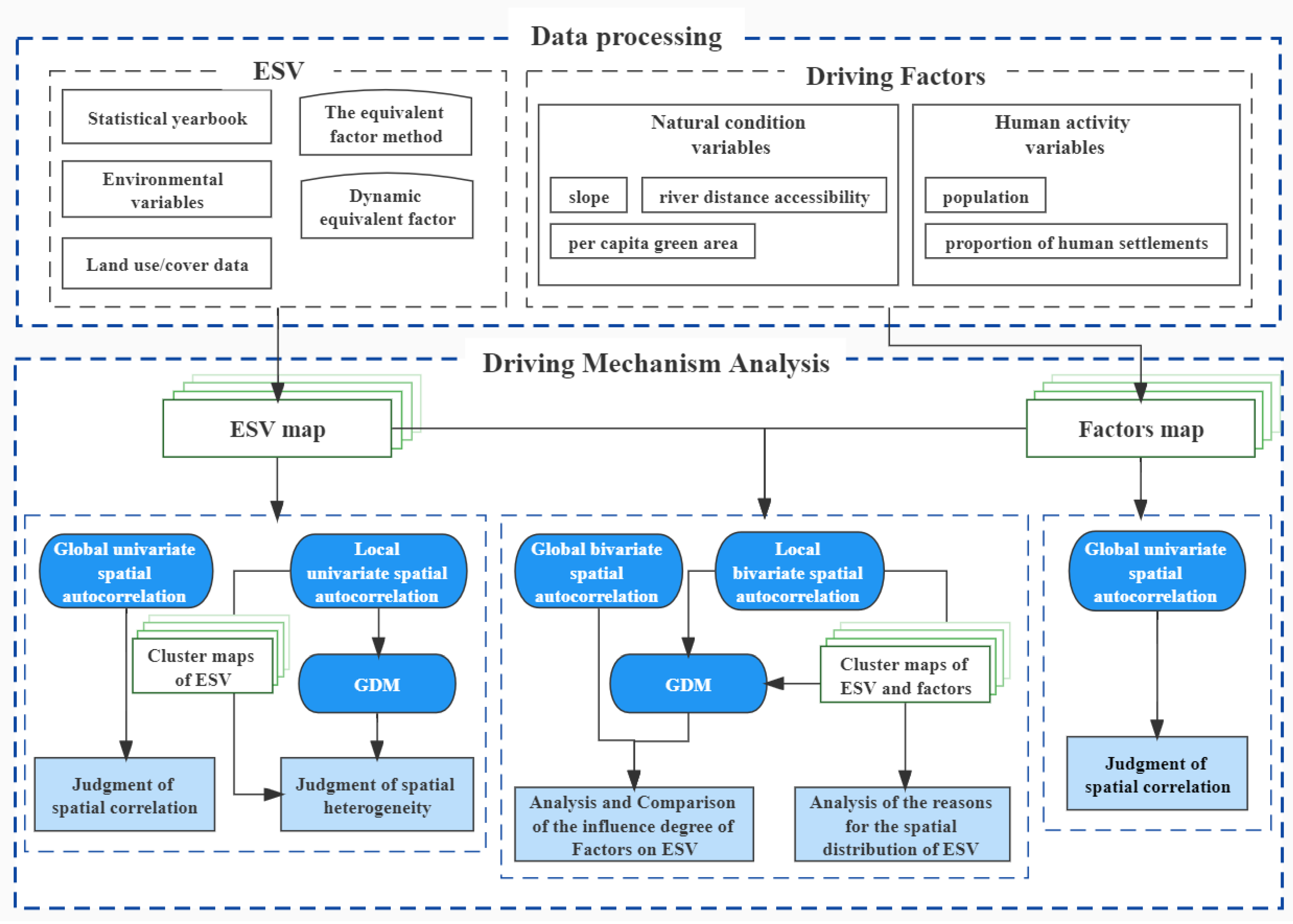
3.4. Research Framework

This section exposed the reader to this study’s primary methods and objectives. The framework of this study included two separate modules (Figure 3): data processing and driving mechanism analysis.
The data processing module included the ESV-related data processing and the Driving factors-related data processing submodules. The dynamic equivalence factor was obtained based on the equivalence factor table and environmental variables. Dynamic equivalence factor and statistical yearbook were used for interannual ESV estimation, and land use/cover data was used for spatial ESV mapping. In the Driving factors-related data processing section, the original raster or vector data of natural conditions and human activity variables were subjected to spatial analysis and processing, and then mapping was performed. For more details, see Section 2.3.
In the driving mechanism module, global spatial autocorrelation analysis was performed on ESV and driving factors to verify whether they have a significant spatial correlation. Then, local spatial autocorrelation analysis was performed on ESV, and GDM was used to explore the spatial heterogeneity of ESV. Secondly, bivariate-based spatial autocorrelation analysis was used to explore the reasons for forming the spatial distribution of ESV. Then, the local spatial correlation patterns obtained by the local bivariate-based autocorrelation analysis were used to stratify the study area, and GDM was used to investigate the impact of driving factors on ESV. Finally, the results of the two analysis methods were compared to judge whether the GDM analysis method was effective.

4. Results and Analysis

4.1. The Spatiotemporal Characteristics of ESV

Calculated and aggregated according to Formula (1), the total value of ecosystem services in the study area in 2005, 2010, 2015, and 2018 were 3649.4923, 3684.7445, 3664.2962, and 3665.7068 million US dollars, respectively. There was an upward trend from 2005–2010 and 2015–2018 and a clear downward trend from 2010-2015. Overall, from 2005 to 2018, the total value of ESV in the Liuxi River Basin experienced a volatile increase, an increase of approximately 16.2145 US million dollars. It shows that the environmental conditions of the basin have been effectively improved during the study period, and this trend can offset the adverse effects of economic development and human activities to a certain extent.
In order to better observe and analyze the spatial distribution of ESV and its changes, the natural discontinuous point method was used to divide ESV into five grades: well, relatively well, ordinary, relatively weak, and weak. Figure 4a–d show that there were spatial differences in the distribution of ESV in 2005, 2010, 2015, and 2018. The well and relatively well areas were mainly distributed in the forest cover area in the northeastern part of the basin. The highest values appeared in the water body and surrounding areas and maintained a dominant state. However, weak and relatively weak areas were mainly distributed in urban areas in the central and southwest of the basin, with the lowest values appearing in the built-up areas in the southwest. Figure 4e shows the statistics of the ESV area at different levels. During the study period, the total area at the relatively good level was the largest, and the total area at the poor level was the smallest. Figure 4f shows the temporal changes of the five ESV levels. The combined area of the well and relatively well levels was the smallest in 2015 and the largest in 2010, while the combined area of the ESV weak and relatively weak levels was the largest in 2015 and the smallest in 2005. By combining the total value of ecosystem services in different periods, it was estimated that 2010 was the best year while 2015 was the worst year for the ecological environment of the basin.
According to Formula (3), the global Moran’s I index (by the significance test) of ESV in 2005, 2010, 2015, and 2018 were 0.568, 0.550, 0.552, and 0.554, respectively, there was a significant spatial aggregation phenomenon, and the degree of aggregation first decreased and then increased. According to Formula (7), ESV’s q-statistics (by the significance test) in 2005, 2010, 2015, and 2018 were 0.5415, 0.5376, 0.5382, and 0.5388, respectively, significant spatial stratified heterogeneity phenomenon, and the degree of heterogeneity first decreased and then increased. The clustering pattern of ESV obtained by Formula (4) also indicates that ESV has apparent differences in different spatial locations and has the characteristics of two-pole spatial aggregation. ESV high-value accumulation areas occurred in the northeast, and ESV low-value accumulation areas occurred in the central and southwest. The low-value accumulation areas were contiguous, whose area was larger than the high-value accumulation areas.

4.2. Correlation Analysis Results of Spatial Factors

Considering that the information overlap between factors may affect the analysis of the driving relationship between them and ESV, the stepwise regression method of SPSS was used to test whether there was multicollinearity among the selected factors. The regression equation can pass the test only when p < 0.01. Table 3 shows that there was no multicollinearity problem (variance inflation factor (VIF) < 10 or tolerance (TOL) > 0.1) among the factors during the study period, indicating that they were independent of each other. In addition, according to Formula (4), the factors themselves all showed a statistically significant (p < 0.05) spatial autocorrelation (Moran’s I > 0.65), see Table 4. Therefore, further probing the five factors’ spatial influence on ESV was necessary.

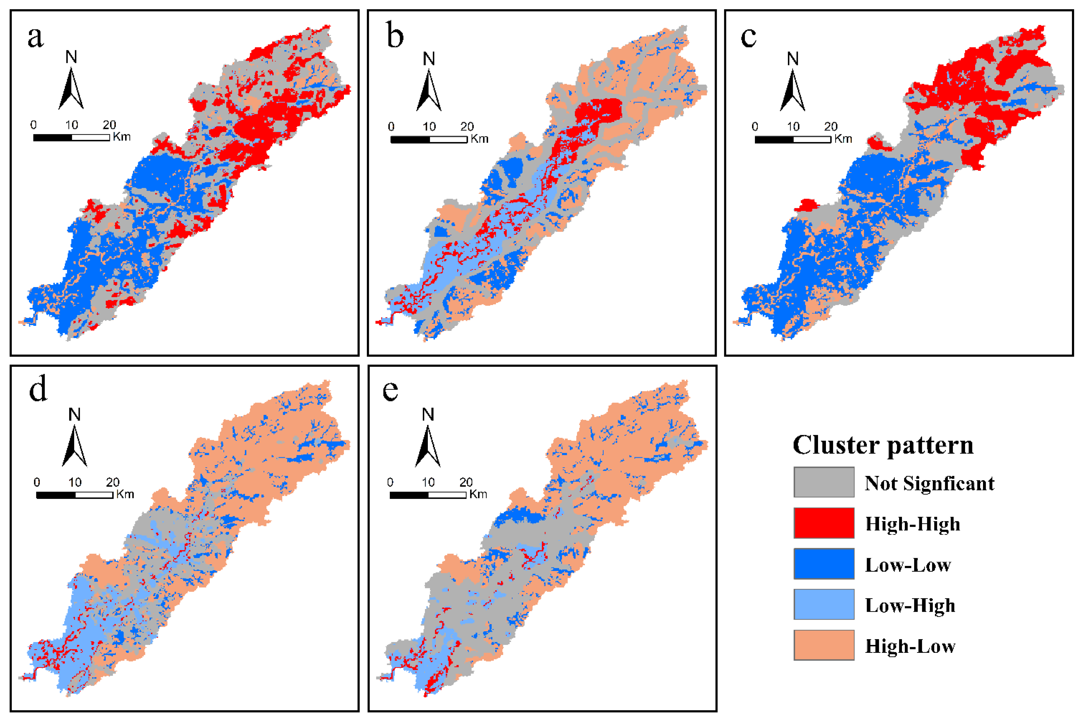
4.3. Moran Bivariate Analysis

According to Formula (5), the global bivariate Moran’s I between ESV and five spatial factors was calculated by Geoda software. All Moran’s I were statistically significant (p < 0.01) (Figure 5). There were spatial correlations between ESV and the five spatial factors, and the degree of correlation differs. There was a positive spatial correlation between ESV and SLO, ESV and GRE, indicating spatial agglomeration among them. The bivariate Moran’s I value of ESV and SLO was stable at around 0.2, and the bivariate Moran’s I value of ESV and GRE increased from 0.199 in 2005 to 0.227 in 2018. Its spatial correlation showed an increasing trend. At the same time, there was a negative spatial correlation between ESV and UR, POP, and RDC, indicating spatial dispersion among them. The negative correlation between ESV and UR was always the strongest and showed an increasing trend; at the same time, the negative spatial correlation between ESV and POP showed a trend of “increase, decrease and increase”; in addition, the bivariate Moran’s I of ESV and RDC was close to 0, implying their spatial correlation was insignificant. Overall, the global bivariate Moran’s I absolute values of the mean order over the study period were: UR > GRE > SLO > POP > RDC.
According to Formula (6), the LISA clustering map was generated by GeoDa’s bivariate LISA method, and the local spatial correlation between ESV and each factor was visualized, see Figure 6. Taking 2018 as an example, by observing the aggregation of HH, LL, HL, and LH values in the area, ESV and SLO can be found. The LL accumulation areas between ESV and GRE were concentrated in the middle and southwest of the basin, covering a large area and distributed in contiguous areas. In these areas, units with low ESV values were surrounded by units with low elevation, a slight SLO, and a small GRE. The HH accumulation areas between ESV and SLO, GRE, and RDC were primarily spread in the northeastern part of the basin, where high ESV values were surrounded by high SLO and high GRE close to the river. The HH and HL accumulation areas of ESV and RDC were mainly distributed in the basin northeast with sufficient water supply.
In contrast, their LH accumulation areas were distributed on both sides of the mainstream of the Liuxi River. These areas were mainly paddy fields and construction land, resulting in significant water demand. In addition, the HL accumulation areas between ESV and UR, ESV and POP were distributed in the northeastern part of the basin, and units surround the units with high ESV values with small UR and small POP; at the same time, their LH accumulation areas concentrated in the basin’s central and southwestern regions, where construction land was concentrated, social and economic activities were frequent. The increase in urbanization level may lead to a decrease in the ESV value of their surrounding units.

4.4. GDM Factor Detection

4.4.1. Single Factor Detection

According to the clustering results in Figure 6, the study area was stratified, and the q-statistic of the explanation degree of five factors for the spatial differentiation of ESV was obtained through the GDM factor detector. The significance test p values of the five factors all reached the significance level of 1%, indicating that ESV resulted from many factors’ action (Figure 7). Five spatial factors explained the spatial heterogeneity of ESV in the whole basin to different degrees; that is, each factor was significantly consistent with the spatial distribution of ESV. Among them, the q-statistic of GRE remained above 0.42, and its explanatory power for the spatial heterogeneity of ESV has always been the strongest. The q-statistic of the SLO was stable above 0.41, and its explanatory power showed an upward trend. Both UR and the explanatory power of RDC were rising. Compared with other factors, the explanatory power of POP was the weakest, showing a trend of “first increase and then decrease.” Overall, the q-statistics of the five factors during the study period were sorted by mean: GRE > SLO > UR > RDC > POP.

4.4.2. Two-Factor Interaction Detection

Through the GDM interaction detector, the q statistic of the explanatory degree of the interaction between the two factors on the spatial differentiation of ESV was obtained (significance test p-value < 0.01). Table 5 lists the explanatory power level in the top four main interactions. It can be found that the interaction between factors had a significant two-factor enhancement or nonlinear enhancement effect on the explanatory power of the spatial differentiation of ESV, which indicated that the synergistic effect of the two factors exceeded the individual effect of a single factor or the cumulative effect of the two factors. In the whole basin, the interaction between SLO and RDC had the most potent explanatory power for the spatial differentiation of ESV (q statistic > 0.49), and it showed an upward trend; the interaction between SLO and UR provided the most potent explanatory power. The explanatory power of the interaction between SLO and GRE, SLO, and POP was declining relative to other interactions.

5. Discussion

The highlight of this study was the use of bivariate Moran’s I clustering results to stratify the study area. This stratification method made the GDM detection results find that five factors have significant explanatory power for the spatial distribution pattern of ESV. Compared with the stratification of the study area using the univariate Moran’s I clustering results, the explanatory power of the five factors for ESV was significantly enhanced after the bivariate Moran’s I clustering results were stratified. At the same time, when spatial correlation and heterogeneity were not considered, only the natural discontinuity method on attribute values, K-means clustering method, and equal interval classification method were used to stratify the study area [44,52], the q-statistics of the five factors obtained by GDM were all small, resulting in their loss of explanatory power for ESV. In addition, the comparison between different factors can provide a direction of tendencies for ecological protection policy trade-offs. However, existing research on ESV has not been able to determine the priority of the importance levels of various factors. However, this study not only identified the spatial dependence characteristics between each influencing factor and ESV at the grid scale but also mined the importance order and temporal change of the influence degree of each factor on ESV by combining GDM. The results were beneficial in providing ecological protection recommendations for the basin.

5.1. The Reason for the Formation of the Spatial Distribution of ESV

This study found significant spatial autocorrelation and spatial heterogeneity of ESVs in the Liuxi River Basin. Therefore, identifying the spatial clustering pattern between ESV and impact factors helped explore the reasons for forming the spatial distribution characteristics of this ecological environment quality [32]. The following conclusions can be inferred by combining the spatial distribution of ESV with the local bivariate spatial correlation patterns. The formation of high-value ESV accumulation areas in the northeastern river basin may be affected by factors such as excellent GRE, high RDC, and high SLO, which exert positive external forces on ESV. It was located in a hilly area with a wide area of forests and rivers. Due to natural conditions such as temperature and topography, the cost of urban construction and economic development was relatively high, which protected ecosystem services. The formation of low-value accumulation areas in southwestern urban areas may be affected by factors such as the large UR, the large POP, and the high RDC, which exerted opposing external forces on ESV. Most of these areas were located in plains and areas near rivers. The level of urbanization was high, and the surface coverage was mainly impervious surface. Compared with other types of land cover, the surface evapotranspiration was lower, and the natural ecosystem was quickly disturbed by the development of human society [26], adversely affecting ecosystem services. In addition, Cui et al. [33] conducted a study on Zhuhai, China, and found that ecosystem health was negatively connected with the urbanization of the economy, construction area, and population.

5.2. Driving Mechanism of ESV

The explanatory power of each driving factor detected by GDM factors stratified was more substantial than that of using the global bivariate-based spatial autocorrelation analysis, and the relative importance of different factors on the explanatory power of ESV changed.
The GDM results showed that the GRE had the most decisive influence on ESV, and the natural barrier it provided for ESV protection is significant to maintaining the dominant state of ESV; The influence of SLO on ESV was relatively stable, and it played an essential role in protecting the basin ecosystem from human disturbance [29]; the impact of RDC on ESV was stable; the impact of UR on ESV showed a gradually increasing trend. Peng et al. [27] also indicated that land urbanization had a more significant and direct influence on ESV than population urbanization. In addition, POP had the weakest and most fluctuating impact on ESV during the study period, indicating its effect on ESV was unstable. This finding conflicts with studies by Wang et al [29] in the Pearl River Delta region, which found that population density was becoming increasingly important. In addition, according to the q-statistic of the interaction between two factors, it can be found that the interaction between factors had a significant two-factor enhancement or nonlinear enhancement effect on the explanatory power of the spatial heterogeneity of ESV. The interaction between the three natural conditions has always been the dominant factor affecting ESV. In addition, in recent years (2015–2018), the interaction between urbanization level and natural conditions has become significant. It suggested that the effects of land urbanization gradually played a leading role in the combined effects [39]. Studies have also shown that socioeconomic variables serve as links and reinforce other variables in regions with low and moderate ecosystem health levels [39].

5.3. Policy Recommendations for the Liuxi River Basin

In light of the study’s conclusions, the following suggestions were put forward for the ecologically sustainable development planning of the Liuxi River Basin: (1) As the ecological environment energy guarantees the area of the whole river basin, the high-value ESV accumulation areas can be maintained green coverage and protect biodiversity by delimiting nature reserves and continue to play its beneficial role. In contrast, as the main contributor to the deterioration of ecological environment health, ESV low-value accumulation areas can adopt ecological conservation projects such as returning farmland to forests to improve and manage their ecosystem services, thereby promoting the healthy restoration of their ecosystems. (2) To maintain an excellent natural ecosystem in the entire basin area, future protection measures in the basin should focus on human settlements. Due to the excellent water conservation conditions and biodiversity in the area near the river, proper control of the expansion rate of human settlements near the river and the avoidance of unreasonable reclamation is conducive to enhancing the organization of the natural ecosystem. (3) The influence of human economic activities on the service value of the basin ecosystem was gradually increasing. In the future, it is necessary to focus on balancing the relationship between economic growth and environmental protection so that the ecological environment of the basin can be coordinated with economic development and more suitable for human habitation.

5.4. Study Limitations and Prospects for Future Research

Although research on the driving mechanisms of basin ecosystem services has progressed, further study must address the following issues. First, there is an intimate interaction between humans and the environment in the basin and an intricate coupling between economic development and the ecological environment. In this case, future research needs to incorporate more diverse socioeconomic data for analysis. Furthermore, this research only evaluated the spatial distribution of ESV, ignoring detailed changes over time. Although the temporal changes of small basins in shorter years were not necessarily noticeable, further mining the temporal characteristics of multi-source geographic data is needed to capture detailed changes. Therefore, it is necessary to continuously pay attention to the dynamic process of the driving mechanism, such as capturing trends through long-term series models and making scenario simulation predictions. Finally, treating a small basin as a single study area does not provide a clear understanding of the uniqueness of the area. Different basin regions may produce very different results of the driving mechanism of ESV, and only a comparative analysis of multiple basins can learn from each other. Future research can add a comparative analysis of ESV drivers in multiple regions, supplying a scientific foundation for comprehending and improving management practices.

6. Conclusions

This study used the grid of 250 m ∗ 250 m as the research unit. The value equivalent method was used to estimate the ESV of the Liuxi River Basin in 2005, 2010, 2015, and 2018 and obtained ESV’s temporal and spatial distribution. Based on the principles of spatial correlation and heterogeneity. We explored the relationship between ESV and five potential spatial driving factors. Its main research conclusions are: (1) The total value of ecosystem services in the Liuxi River Basin experienced an increase in volatility in the time series from 2005 to 2018, with an increase of about 16.2145 million US dollars. (2) The spatial autocorrelation and spatial heterogeneity of ESV within the basin were highly significant. ESV high-value aggregation areas were mainly distributed in northeastern mountainous regions, and ESV, SLO, GRE, and RDC had a positive spatial correlation. ESV low-value aggregation areas were concentrated in the southwestern urban areas, and there was a negative spatial correlation between ESV and the UR, POP, and RDC. (3) The spatial distribution characteristics of ESV were affected by various driving factors to varying degrees. The order of their degree of influence on ESV during the study period was GRE > SLO > UR > RDC > POP. (4) The interaction between factors had a significant two-factor enhancement or nonlinear enhancement effect on the explanatory power of the spatial distribution of ESV. The interaction of SLO and RDC, SLO and UR has been the strongest during the study period and showed an upward trend. (5) Compared with traditional stratification methods, we used the local bivariate spatial pattern of ESV and influencing factors for spatial heterogeneity stratification, which made each factor’s capacity for an explanation for ESV significant in the basin. This study considered both the spatial correlation and heterogeneity of ESV and driving factors and determined the priority of the influence degree of the factors of ESV in the basin. The research results are expected to support the scientific decision to alleviate the contradiction in the basin between human activities and environmental protection.

Author Contributions

X.D.: Conceptualization; Methodology; Resources; Formal Analysis; Writing—Original draft; Y.S.: Conceptualization; Supervision; Writing—Reviewing and Editing; X.T.: Writing—Reviewing and Editing; J.M.: Formal Analysis; Writing—Original draft. All authors have read and agreed to the published version of the manuscript.

Funding

This research received no external funding.

Informed Consent Statement

Not applicable.

Data Availability Statement

Data is contained within the article.

Conflicts of Interest

The authors declare no conflict of interest.

References

  1. Tian, Y.Y.; Zhou, D.Y.; Jiang, G.H. Conflict or Coordination? Multiscale assessment of the spatio-temporal coupling relationship between urbanization and ecosystem services: The case of the Jingjinji Region, China. Ecol. Indic. 2020, 117, 14. [Google Scholar] [CrossRef]
  2. Braat, L.C.; de Groot, R. The ecosystem services agenda:bridging the worlds of natural science and economics, conservation and development, and public and private policy. Ecosyst. Serv. 2012, 1, 4–15. [Google Scholar] [CrossRef] [Green Version]
  3. Rapport, D.J.; Costanza, R.; McMichael, A.J. Assessing ecosystem health. Trends Ecol. Evol. 1998, 13, 397–402. [Google Scholar] [CrossRef]
  4. Boithias, L.; Terrado, M.; Corominas, L.; Ziv, G.; Kumar, V.; Marques, M.; Schuhmacher, M.; Acuna, V. Analysis of the uncertainty in the monetary valuation of ecosystem services--A case study at the river basin scale. Sci. Total Environ. 2016, 543, 683–690. [Google Scholar] [CrossRef]
  5. Costanza, R.; d’Arge, R.; de Groot, R.; Farber, S.; Grasso, M.; Hannon, B.; Limburg, K.; Naeem, S.; Oneill, R.V.; Paruelo, J.; et al. The value of the world’s ecosystem services and natural capital. Nature 1997, 387, 253–260. [Google Scholar] [CrossRef]
  6. Wang, X.; Dong, X.; Liu, H.; Wei, H.; Fan, W.; Lu, N.; Xu, Z.; Ren, J.; Xing, K. Linking land use change, ecosystem services and human well-being: A case study of the Manas River Basin of Xinjiang, China. Ecosyst. Serv. 2017, 27, 113–123. [Google Scholar] [CrossRef]
  7. Xie, G.; Zhang, C.; Zhen, L.; Zhang, L. Dynamic changes in the value of China’s ecosystem services. Ecosyst. Serv. 2017, 26, 146–154. [Google Scholar] [CrossRef]
  8. Chen, W.; Zeng, J.; Zhong, M.; Pan, S. Coupling Analysis of Ecosystem Services Value and Economic Development in the Yangtze River Economic Belt: A Case Study in Hunan Province, China. Remote Sens. 2021, 13, 1552. [Google Scholar] [CrossRef]
  9. Peng, J.; Liu, Y.; Li, T.; Wu, J. Regional ecosystem health response to rural land use change: A case study in Lijiang City, China. Ecol. Indic. 2017, 72, 399–410. [Google Scholar] [CrossRef]
  10. Lin, W.P.; Xu, D.; Guo, P.P.; Wang, D.; Li, L.B.; Gao, J. Exploring variations of ecosystem service value in Hangzhou Bay Wetland, Eastern China. Ecosyst. Serv. 2019, 37, 9. [Google Scholar] [CrossRef]
  11. Sun, X.; Lu, Z.M.; Li, F.; Crittenden, J.C. Analyzing spatio-temporal changes and trade-offs to support the supply of multiple ecosystem services in Beijing, China. Ecol. Indic. 2018, 94, 117–129. [Google Scholar] [CrossRef]
  12. Wang, J.L.; Zhou, W.Q.; Pickett, S.T.A.; Yu, W.J.; Li, W.F. A multiscale analysis of urbanization effects on ecosystem services supply in an urban megaregion. Sci. Total Environ. 2019, 662, 824–833. [Google Scholar] [CrossRef]
  13. Zhang, Y.S.; Lu, X.; Liu, B.Y.; Wu, D.T.; Fu, G.; Zhao, Y.T.; Sun, P.L. Spatial relationships between ecosystem services and socioecological drivers across a large-scale region: A case study in the Yellow River Basin. Sci. Total Environ. 2021, 766, 16. [Google Scholar] [CrossRef]
  14. Li, T.; Lü, Y. A review on the progress of modeling techniques in ecosystem services. Acta Ecol. Sin. 2018, 38, 5287–5296. [Google Scholar]
  15. Xie, G.D.; Lu, C.X.; Leng, Y.F.; Zheng, D.U.; Li, S.C. Ecological assets valuation of the Tibetan Plateau. J. Nat. Resour. 2003, 18, 189–196. [Google Scholar] [CrossRef]
  16. Yan, F.Q.; Zhang, S.W. Ecosystem service decline in response to wetland loss in the Sanjiang Plain, Northeast China. Ecol. Eng. 2019, 130, 117–121. [Google Scholar] [CrossRef]
  17. Li, Q.; Yu, Y.; Catena, M.R.; Ahmad, S.; Jia, H.; Guan, Y. Multifactor-based spatio-temporal analysis of effects of urbanization and policy interventions on ecosystem service capacity: A case study of Pingshan River Catchment in Shenzhen city, China. Urban For. Urban Green. 2021, 64, 127263. [Google Scholar] [CrossRef]
  18. Wang, Z.; Mao, D.; Li, L.; Jia, M.; Dong, Z.; Miao, Z.; Ren, C.; Song, C. Quantifying changes in multiple ecosystem services during 1992-2012 in the Sanjiang Plain of China. Sci. Total Environ. 2015, 514, 119–130. [Google Scholar] [CrossRef]
  19. He, J.; Pan, Z.; Liu, D.; Guo, X. Exploring the regional differences of ecosystem health and its driving factors in China. Sci. Total Environ. 2019, 673, 553–564. [Google Scholar] [CrossRef]
  20. Luo, Q.; Zhou, J.; Li, Z.; Yu, B. Spatial differences of ecosystem services and their driving factors: A comparation analysis among three urban agglomerations in China’s Yangtze River Economic Belt. Sci. Total Environ. 2020, 725, 138452. [Google Scholar] [CrossRef]
  21. Lyu, R.; Clarke, K.C.; Zhang, J.; Feng, J.; Jia, X.; Li, J. Spatial correlations among ecosystem services and their socio-ecological driving factors: A case study in the city belt along the Yellow River in Ningxia, China. Appl. Geogr. 2019, 108, 64–73. [Google Scholar] [CrossRef]
  22. Ma, S.; Wang, L.-J.; Jiang, J.; Chu, L.; Zhang, J.-C. Threshold effect of ecosystem services in response to climate change and vegetation coverage change in the Qinghai-Tibet Plateau ecological shelter. J. Clean. Prod. 2021, 318, 128592. [Google Scholar] [CrossRef]
  23. Wang, X.; Liu, G.; Xiang, A.; Qureshi, S.; Li, T.; Song, D.; Zhang, C. Quantifying the human disturbance intensity of ecosystems and its natural and socioeconomic driving factors in urban agglomeration in South China. Environ. Sci. Pollut. Res. 2021, 29, 11493–11509. [Google Scholar] [CrossRef]
  24. Deng, C.X.; Liu, J.Y.; Nie, X.D.; Li, Z.W.; Liu, Y.J.; Xiao, H.B.; Hu, X.Q.; Wang, L.X.; Zhang, Y.T.; Zhang, G.Y.; et al. How trade-offs between ecological construction and urbanization expansion affect ecosystem services. Ecol. Indic. 2021, 122, 12. [Google Scholar] [CrossRef]
  25. Dai, X.; Wang, L.C.; Huang, C.B.; Fang, L.L.; Wang, S.Q.; Wang, L.Z. Spatio-temporal variations of ecosystem services in the urban agglomerations in the middle reaches of the Yangtze River, China. Ecol. Indic. 2020, 115, 11. [Google Scholar] [CrossRef]
  26. Han, R.; Feng, C.C.E.; Xu, N.Y.; Guo, L. Spatial heterogeneous relationship between ecosystem services and human disturbances: A case study in Chuandong, China. Sci. Total Environ. 2020, 721, 11. [Google Scholar] [CrossRef]
  27. Peng, J.; Tian, L.; Liu, Y.; Zhao, M.; Hu, Y.; Wu, J. Ecosystem services response to urbanization in metropolitan areas: Thresholds identification. Sci. Total Environ. 2017, 607–608, 706–714. [Google Scholar] [CrossRef]
  28. Xing, L.; Zhu, Y.; Wang, J. Spatial spillover effects of urbanization on ecosystem services value in Chinese cities. Ecol. Indic. 2021, 121, 107028. [Google Scholar] [CrossRef]
  29. Wang, S.; Liu, Z.; Chen, Y.; Fang, C. Factors influencing ecosystem services in the Pearl River Delta, China: Spatiotemporal differentiation and varying importance. Resour. Conserv. Recycl. 2021, 168, 105477. [Google Scholar] [CrossRef]
  30. He, Y.; Kuang, Y.; Zhao, Y.; Ruan, Z. Spatial Correlation between Ecosystem Services and Human Disturbances: A Case Study of the Guangdong-Hong Kong-Macao Greater Bay Area, China. Remote Sens. 2021, 13, 1174. [Google Scholar] [CrossRef]
  31. Zhang, Y.; Liu, Y.F.; Zhang, Y.; Liu, Y.; Zhang, G.X.; Chen, Y.Y. On the spatial relationship between ecosystem services and urbanization: A case study in Wuhan, China. Sci. Total Environ. 2018, 637, 780–790. [Google Scholar] [CrossRef]
  32. Shi, Y.; Feng, C.-C.; Yu, Q.; Guo, L. Integrating supply and demand factors for estimating ecosystem services scarcity value and its response to urbanization in typical mountainous and hilly regions of south China. Sci. Total Environ. 2021, 796, 149032. [Google Scholar] [CrossRef]
  33. Cui, N.; Feng, C.C.; Han, R.; Guo, L. Impact of Urbanization on Ecosystem Health: A Case Study in Zhuhai, China. Int. J. Environ. Res. Public Health 2019, 16, 4717. [Google Scholar] [CrossRef] [Green Version]
  34. Ling, H.; Yan, J.; Xu, H.; Guo, B.; Zhang, Q. Estimates of shifts in ecosystem service values due to changes in key factors in the Manas River basin, northwest China. Sci. Total Environ. 2019, 659, 177–187. [Google Scholar] [CrossRef]
  35. Dutilleul, P. Spatio-Temporal Heterogeneity: Concepts and Analyses; Cambridge University Press: Cambridge, UK; New York, NY, USA, 2011. [Google Scholar]
  36. Wang, J.-F.; Zhang, T.-L.; Fu, B.-J. A measure of spatial stratified heterogeneity. Ecol. Indic. 2016, 67, 250–256. [Google Scholar] [CrossRef]
  37. Fu, J.; Zhang, Q.; Wang, P.; Zhang, L.; Tian, Y.; Li, X. Spatio-Temporal Changes in Ecosystem Service Value and Its Coordinated Development with Economy: A Case Study in Hainan Province, China. Remote Sens. 2022, 14, 970. [Google Scholar] [CrossRef]
  38. Wang, J.; Xu, C. Geodetector: Principle and prospective. Acta Geogr. Sin. 2017, 72, 116–134. [Google Scholar]
  39. Fang, L.; Wang, L.; Chen, W.; Sun, J.; Cao, Q.; Wang, S.; Wang, L. Identifying the impacts of natural and human factors on ecosystem service in the Yangtze and Yellow River Basins. J. Clean. Prod. 2021, 314, 127995. [Google Scholar] [CrossRef]
  40. Wang, X.G.; Yan, F.Q.; Su, F.Z. Impacts of Urbanization on the Ecosystem Services in the Guangdong-Hong Kong-Macao Greater Bay Area, China. Remote Sens. 2020, 12, 3269. [Google Scholar] [CrossRef]
  41. Zhenjie, Z.; Zibo, Y.; Bingjun, L. Analysis of Spatio-temporal Evolution of Land Use and Landscape Pattern in Liuxi River Basin Driven by Rapid Urbanization. Pearl River 2020, 41, 11. [Google Scholar]
  42. Gedo, H.W.; Morshed, M.M. Inadequate accessibility as a cause of water inadequacy: A case study of Mpeketoni, Lamu, Kenya. Water Policy 2013, 15, 598–609. [Google Scholar] [CrossRef]
  43. Lorenz, C.; Tourian, M.J.; Devaraju, B.; Sneeuw, N.; Kunstmann, H. Basin-scale runoff prediction: An Ensemble Kalman Filter framework based on global hydrometeorological data sets. Water Resour. Res. 2015, 51, 8450–8475. [Google Scholar] [CrossRef] [Green Version]
  44. Yang, J.; Xie, B.; Zhang, D. Spatial-temporal evolution of habitat quality and its influencing factors in the Yellow River Basin based on InVEST model and GeoDetector. J. Desert Res. 2021, 41, 12. [Google Scholar]
  45. Nan, B.; Yang, Z.; Bi, X.; Fu, Q.; Li, B. Spatial-temporal correlation analysis of ecosystem services value and human activities-a case study of Huayang Lakes area in the middle reaches of Yangtze River. China Environ. Sci. 2018, 38, 3531–3541. [Google Scholar]
  46. Gong, P.; Li, X.; Zhang, W. 40-Year (1978–2017) human settlement changes in China reflected by impervious surfaces from satellite remote sensing. Sci. Bull. 2019, 64, 756–763. [Google Scholar] [CrossRef]
  47. Xiong, J.N.; Li, W.; Zhang, H.; Cheng, W.M.; Ye, C.C.; Zhao, Y. Selected Environmental Assessment Model and Spatial Analysis Method to Explain Correlations in Environmental and Socio-Economic Data with Possible Application for Explaining the State of the Ecosystem. Sustainability 2019, 11, 4781. [Google Scholar] [CrossRef] [Green Version]
  48. Anselin, L. GeoDa 0.9 User’s Guide; Spatial Analysis Laboratory, Department of Agricultural and Consumer Economics, University of Illinois Urbana-Champaign: Urbana, IL, USA, 2003. [Google Scholar]
  49. Hu, X.; Xu, H. A new remote sensing index for assessing the spatial heterogeneity in urban ecological quality: A case from Fuzhou City, China. Ecol. Indic. 2018, 89, 11–21. [Google Scholar] [CrossRef]
  50. Anselin, L.; Rey, S.J. Modern Spatial Econometrics in Practice: A Guide to GeoDa, GeoDaSpace and PySAL; GeoDa Press LLC.: Chicago, IL, USA, 2014. [Google Scholar]
  51. Anselin, L. Thirty years of spatial econometrics. Pap. Reg. Sci. 2010, 89, 3–25. [Google Scholar] [CrossRef]
  52. Ren, Y.; Deng, L.Y.; Zuo, S.D.; Song, X.D.; Liao, Y.L.; Xu, C.D.; Chen, Q.; Hua, L.Z.; Li, Z.W. Quantifying the influences of various ecological factors on land surface temperature of urban forests. Environ. Pollut. 2016, 216, 519–529. [Google Scholar] [CrossRef]
Figure 1. Location map of the study area: (a) the location of Guangdong Province in China; (b) the location of Liuxi River Basin in Guangdong Province; (c) the Land use/cover of the study area.
Land 11 01852 g001
Figure 2. Spatial distribution of five factors in 2018: (a) SLO, slope; (b) RDC, river distance accessibility; (c) GRE, per capita green area; (d) UR, the proportion of urban; (e) rural human settlements, POP, population.
Land 11 01852 g002
Figure 3. Research Framework of the Study. ESV, Ecosystem service value; GDM, Geodetector model.
Land 11 01852 g003
Figure 4. Spatial distribution of ESV in (a) 2005, (b) 2010, (c) 2015, and (d) 2018; (e) the percentage of areas with different levels in each year; and (f) the percentage of all grids in each ESV level. ESV, Ecosystem service value.
Land 11 01852 g004
Figure 5. Global Bivariate Moran’s I between ESV and five factors in 2005, 2010, 2015, and 2018. SLO, slope; RDC, river distance accessibility; GRE, per capita green area; UR, the proportion of urban and rural human settlements; POP, population.
Land 11 01852 g005
Figure 6. Bivariate LISA cluster maps between ESV and each factor in 2018: (a) SLP (b) RDC (c) GRE (d) UR (e) POP. SLO, slope; RDC, river distance accessibility; GRE, per capita green area; UR, the proportion of urban and rural human settlements; POP, population.
Land 11 01852 g006
Figure 7. GDM detection q statistic for ESV for five factors. SLO, slope; RDC, river distance accessibility; GRE, per capita green area; UR, the proportion of urban and rural human settlements; POP, population.
Land 11 01852 g007
Table 1. Data source and description.
Data CategoryType of DataResolutionTime (Year)Source
Land use/cover DataRaster data30 m2005, 2010,
2015, 2018
Land cover remote sensing monitoring data set for multi-period land use in China (CNLUCC). Available online: http://www.resdc.cn (assessed on 1 June 2022)
Soil ErodibilityRaster data500 m2005, 2010,
2015
Erosion Area of China in Five-year Increments. Available online: https://doi.org/10.3974/geodb.2021.05.03.V1 (assessed on 1 June 2022)
Digital Elevation Model (DEM)Raster data250 m2000NASA dataset. Available online: https://earthdata.nasa.gov (assessed on 1 June 2022)
Average Monthly PrecipitationRaster data1000 m2005, 2010,
2015, 2018
National Earth System Science Data Center. Available online: http://www.geodata.cn (assessed on 1 June 2022)
PopulationRaster data100 m2005, 2010,
2015, 2018
WordPress Project. Available online: https://www.worldpop.org/ (assessed on 1 June 2022)
Human Settlements (urban and rural)Raster data30 m2005, 2010,
2015, 2017
Impervious surface dataset. Available online: http://data.ess.tsinghua.edu.cn/ (assessed on 1 June 2022)
16-day Net Primary Productivity (NPP)Raster data500 m2005, 2010,
2015, 2018
MODIS/Terra Net Primary Production Gap-Filled Yearly L4 Global 500 m SIN Grid. Available online: https://lpdaac.usgs.gov/products/mod17a3hgfv006/ (assessed on 1 June 2022)
Water SystemVector data/2017National Geographic Information Resources 1:1,000,000 National Basic Geographic Database. Available online: https://www.webmap.cn/ (assessed on 1 June 2022)
Food DataStatistical data/2005, 2010,
2015, 2018
Guangdong Statistical Yearbook. Available online: http://stats.gd.gov.cn/gdtjnj/ (assessed on 1 June 2022)
Table 2. Ecosystem services equivalent coefficients table.
Land Use TypeDry LandPaddy FieldBroadleaf ForestShrubsGrassWetlandWaterConstructionUnused
Ecosystem Classification
Natural environment comprehensive service functionsfood production0.851.360.290.190.380.510.800
raw materials0.40.090.660.430.560.50.2300
gas regulation0.671.112.171.411.971.90.7700.02
climate regulation0.360.576.54.235.213.62.2900
environmental purification0.10.171.931.281.723.65.5500.1
nutrient cycle maintenance 0.120.190.20.130.180.180.0700
biodiversity maintenance0.130.212.411.672.187.872.5500.02
aesthetic landscape0.060.091.060.690.964.731.8900.01
Water source conditions comprehensive service functionswater supply0.02−2.630.340.220.312.598.2900
water regulation0.272.724.743.353.8224.23102.2400.03
Soil conservation service functionsoil conservation1.030.012.651.722.42.310.9300.02
Table 3. Multicollinearity test results in 2005, 2010, 2015, and 2018. SLO, slope; RDC, river distance accessibility; GRE, per capita green area; UR, the proportion of urban and rural human settlements; POP, population.
2005201020152018
pTOLVIFpTOLVIFpTOLVIFpTOLVIF
SLO00.8240991.21344700.7776841.28587000.7551221.32428900.7496371.333978
GRE00.888490 1.125505 00.827045 1.209124 00.814747 1.227374 00.809450 1.235407
UR00.640032 1.562421 00.559448 1.787476 00.562794 1.776848 00.551702 1.812574
POP00.662943 1.508425 00.6116861.63482600.6600701.51499200.6644771.504943
RDC00.8456671.18249900.8388941.19204600.8272111.20888200.8239481.213669
Table 4. Moran’s I for five factors in 2005, 2010, 2015, and 2018. SLO, slope; RDC, river distance accessibility; GRE, per capita green area; UR, the proportion of urban and rural human settlements; POP, population.
SLORDCGREURPOP
20050.7600.9930.9230.6660.857
20100.7600.9930.9240.7510.865
20150.7600.9930.9290.8050.858
20180.760 0.993 0.938 0.815 0.857
Table 5. GDM detection q statistic for interaction between factors on ESV. SLO, slope; RDC, river distance accessibility; GRE, per capita green area; UR, the proportion of urban and rural human settlements; POP, population.
Dominant Interaction2005201020152018
1SLO∩POP0.48914SLO∩RDC0.50597SLO∩RDC0.51013SLO∩RDC0.51112
2SLO∩RDC0.49076SLO∩POP0.49619SLO∩UR0.50460SLO∩UR0.50825
3SLO∩GRE0.48693SLO∩GRE0.49619RDC∩UR0.50105RDC∩UR0.50501
4SLO∩UR0.47996SLO∩UR0.49606SLO∩POP0.50009SLO∩GRE0.50279
Publisher’s Note: MDPI stays neutral with regard to jurisdictional claims in published maps and institutional affiliations.

