Interaction between Tourism Carrying Capacity and Coastal Squeeze in Mazatlan, Mexico

Abstract

While many coastal areas are affected by coastal squeeze, quantitative estimations of this phenomenon are still limited. Ambiguity concerning the degree of coastal squeeze, combined with a lack of knowledge on its interaction with human activities may lead to inadequate and unsuccessful management responses. The objective of the present research was to quantify the degree of coastal squeeze on the highly urbanized coast of Mazatlan, Mexico, and to investigate the relationship between the development of tourism and coastal squeeze from various time perspectives. The Drivers, Exchanges, States of the environment, Consequences, and Responses (DESCR) framework was applied to identify the chronic, negative consequences of dense tourism in the area, together with the assessment of coastal squeeze. A Tourism Load Capacity (TLC) estimation was made and correlated with the DESCR results, showing that coastal squeeze is inversely correlated with tourism load in Mazatlan. The medium-intensity coastal squeeze currently experienced in Mazatlan requires interventions to avoid severe degradation of the ecosystem on which the local tourism industry relies, for which immediate, long-term, and administrative recommendations are given.

1. Introduction

Loss of coastal territory as a result of natural or human activities is a situation faced by most countries with ocean boundaries (Silva et al.) [1]. This threat is the subject of much ongoing research, since it affects both ecosystems and human activities. The intrinsic vulnerability of any coastal zone is undeniable, as these are the most dynamic environments on Earth—the only places where the terrestrial environment, atmosphere, seawater, and freshwater all interact (Silva et al.) [2]. The coastal zone can be delimited as the area between the oceanic boundary of the continental shelf and the first significant topographic change above the maximum storm surge elevation (USACE) [3]. The adaptability of coastal areas, together with the dynamics of the ecosystems they host (wetlands, dunes, and beaches), allow them to control the energy of marine hydrometeorological events and thus, one of the primary services they provide is protection (Silva et al.) [1].

Coastal areas in Europe have always struggled against the loss of territory, particularly in England, where the term coastal squeeze was born (Doody, Tros de Ilarduya) [4,5,6]. This term was initially used to describe the loss of coastline and habitats to sea defences (Pontee et al.) [7]. In general, coastal squeeze has been understood as the process in which hydrometeorological hazards threaten coastal ecosystems through the combination of sea-level rise (SLR) and the presence of rigid barriers which prevent the ecosystems’ adaptation, such as human infrastructure. This situation impedes the terrestrial migration of ecosystems and species as the coast moves inland, and thus they are exposed to local extinction (Martinez et al.) [8]. Natural processes that trigger coastal squeeze include the natural variability in sea level, extreme cyclical events (e.g., storm surges and flooding), and inland landscape morphology, which can function as a static ecological barrier to species migration (Doody) [5]. Known factors contributing to coastal squeeze include global and local climate change and local effects of poorly planned coastal infrastructure (Doody, Pontee et al.) [4,5,7]. The present research considers coastal squeeze as a process in which rising sea levels and other factors, such as hard infrastructure, cause a loss of space in land and sea, and where the ecosystems no longer have the necessary conditions to maintain their essential functions (Silva et al.) [2].

Given its importance and impact on the coasts of many countries, the evaluation of coastal squeeze has been the subject of numerous research efforts. Notable works include those by Jackson et al., Mazaris et al., and Schleupner et al. [9,10,11], who developed methodologies and spatial models to quantify habitat loss. They explained the responses of coastal ecosystems in different study sites (wetlands, mangroves, sea turtle populations, and intertidal organisms). Another example is Torio et al. [12], who developed a coastal squeeze index from a spatial model that can be used along the boundaries of a single wetland and ranks threats faced by multiple wetlands. Coastal squeeze in the state of Veracruz, Mexico, was investigated by Martinez et al. [8]. They considered urban expansion along the coast, an analysis of coastal geodynamics, and a projection of the potential effects of sea-level rise and the distribution of two focal plant species that are endemic to the coastal dunes in Mexico. Using systematic spatial planning, Mills et al. [13] assessed the optimal configuration and the trade-offs involved in SLR adaptation, incorporating spatial models of inundation, urban growth, and ecosystem migration. None of these works included efforts to forecast coastal squeeze, apart from considering some sea-level-rise scenarios. Hildinger and Braun [14] proposed a methodology that considers three main aspects determining the dynamics of coastal squeeze: the geosphere, the biosphere, and the anthropogenic impact. They conducted a small- and large-scale risk analysis to regulate land use, but did not present any quantification or forecast. Luo et al. [15] combined the coastal squeeze index (CSI) and the assessment method proposed by Torio et al. [12] to evaluate the coastal squeeze potential of the Yellow River Delta coastal wetlands in future SLR scenarios. They focused on the effects of slope and impervious surfaces on adjacent uplands with regard to potential wetland migration. This study was applied to a wetland area but not to urbanized coasts. Luo et al. and Ramirez-Vargas et al. [15,16] developed fuzzy-logic-based coastal squeeze indexes to quantify coastal squeeze intensity. They included ecological, geomorphological, and socioeconomic variables. Silva et al. [2] developed the DESCR (Drivers, Exchanges, States, Consequences, and Responses) framework, which examines the relationships between drivers, exchanges, and environmental states to subsequently assess chronic and negative consequences and determine potential responses to combat coastal squeeze. A recurrent gap in all of the cited work is the assessment of coastal squeeze along with possible response actions, including an evaluation of tourism carrying capacity (Cifuentes) [17].

Three main aspects have increased the rise in consciousness regarding coastal erosion: (a) the continuous growth of human coastal settlements, (b) the lack of knowledge on coastline behavior in the short and medium term and (c) the inefficient regulation of coastal urbanization (Silva et al.) [1]. In Mexico, the federal government has expressed interest in developing a strategy to manage all coastal zones and solve the problems faced there. Unfortunately, they have not yet successfully implemented integrated management, so the issues have been addressed individually: that is, in response to the specific needs, or emergencies, of owners or concessionaires (Cortes-Macías et al., Escofet) [18,19]. For the last 50 years, the Mexican coast, particularly along the Caribbean and the Central Pacific, has hosted tourism, residential, and industrial developments. In this time, countless structures have been built with inappropriate designs and with severe impacts on coastal dynamics. The lack of specific regulatory criteria has meant it is impossible to stop or improve poorly planned developments (Silva et al.) [1]. Unfortunately, most anthropic activities affect the coast, directly or indirectly, causing negative consequences on it (Petrişor et al., Senouci and Taibi)) [20,21]. The transcendence of the phenomenon means it is a critical issue; it is induced by the lack of public policies and specific programs to protect and sustain the coastal zone (Huang et al.) [22]. There is an urgent need to establish programs to control, monitor, and predict the behavior of coasts, in order to minimize the physical, ecological, and socioeconomic consequences of their deterioration under different scenarios (natural and anthropogenic).

Given predictions of current and future climate change scenarios and the continuous modification of coastal ecosystems (urbanization), there has been a growing interest in the study of coastal squeeze assessment (Lithgow et al.) [23]. This paper evaluates and quantifies the degree of coastal squeeze occurring at Mazatlan, Mexico. The initial approach to a coastal squeeze intensity forecast was conducted using available historical data and linear models. Next, the tourist carrying capacity was estimated, and a forecast is provided to correlate its evolution with that of the intensity of coastal squeeze. The study site was modeled under different scenarios (past, present, and future) to seek alternatives to reverse the negative trends found. Recommendations for coastal tourism management to avoid increasing coastal squeeze in Mazatlan are proposed.

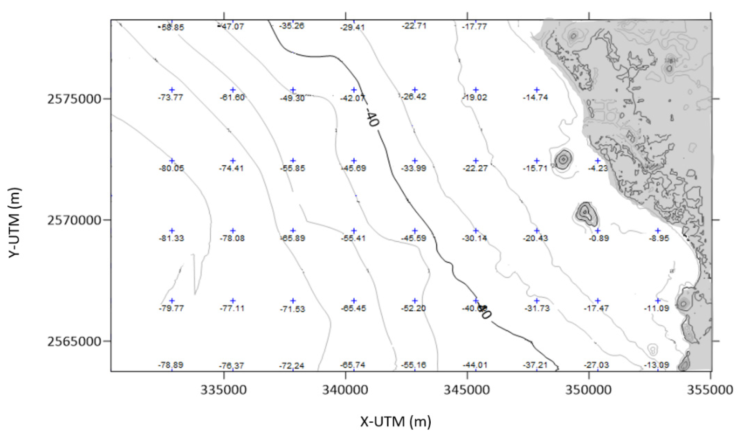
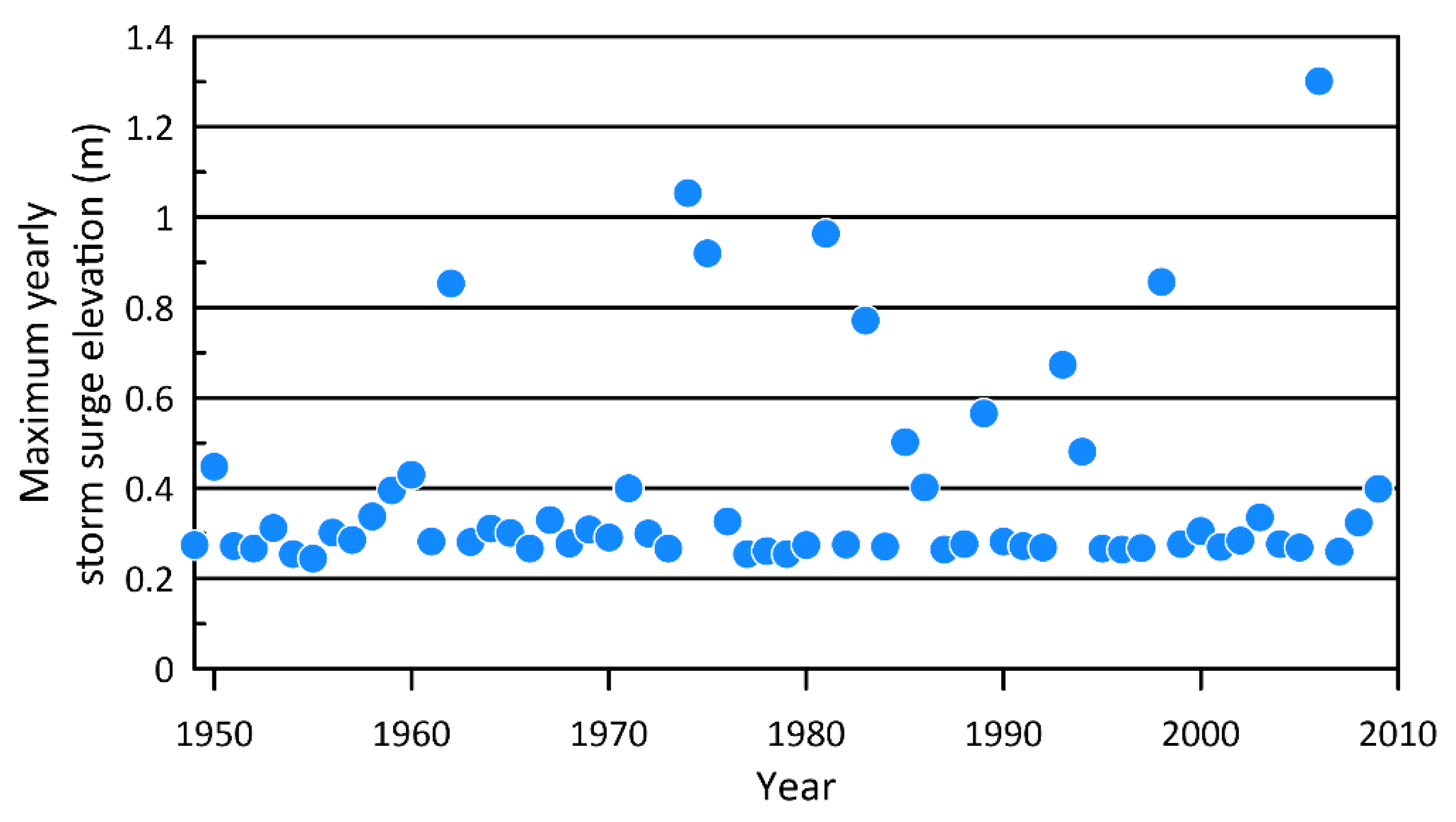
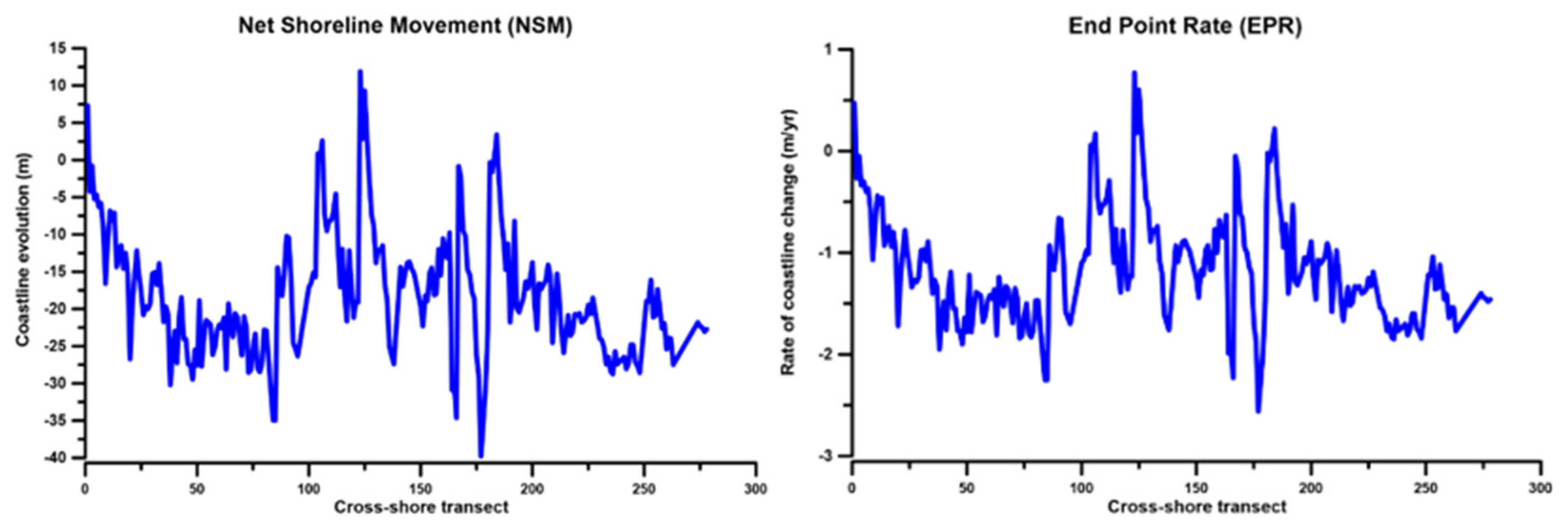
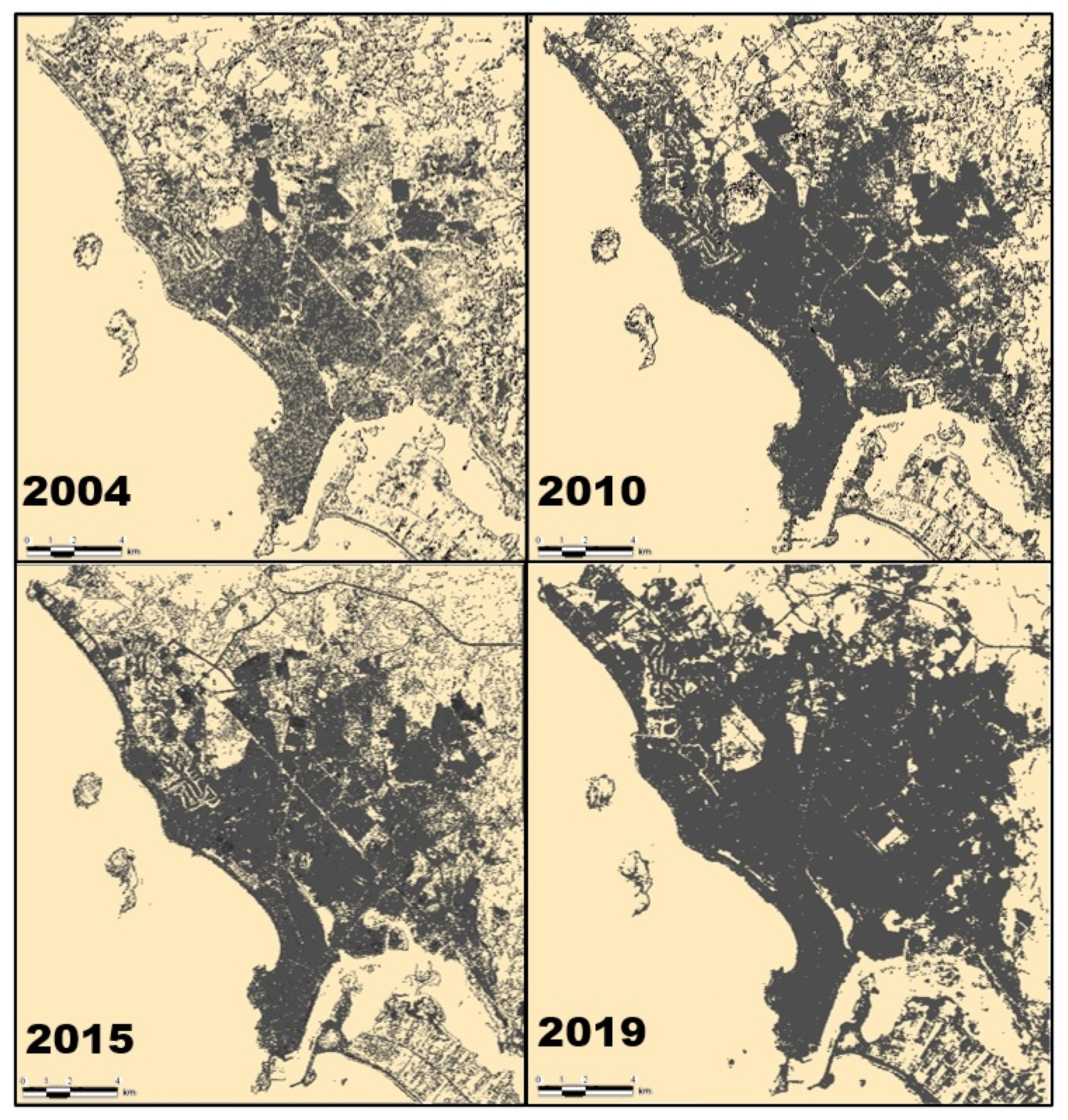
In Section 2 the methods used are presented, including the study site description and the data sources; Section 3 shows the results of coastline evolution, estimation of maximum water elevation, and the assessment of coastal squeeze and tourism carrying capacity in Mazatlan. The discussion and conclusions of our findings are given in Section 4.

2. Methods

2.1. Study Site Description

The coastal unit of Mazatlan, a municipality in Sinaloa, Mexico, is bordered to the north by San Ignacio Municipality and the state of Durango, to the east by Concordia Municipality, to the south by Rosario Municipality, and to the west by the Pacific Ocean (Figure 1). Mazatlan is located between the coordinates 105°46′23″, and 106°30′51″ W and 23°04′25″ and 23°50′22″ N. According to the 2010 census by INEGI [24], Mazatlan has a population of 500,000 and an area of 3068 km² [25].

Mazatlan is one of the chief ports on the Mexican Pacific due to its maritime conditions, celebrated fishing activity, and tourist activities (it was the sixth national “sun and sea” destination in 2014 according to DATATUR [26]). In 2015, Mazatlan received more than 2,177,000 visitors, an 8% growth compared to 2014. The economic revenue from tourism increased 9% from 2014 to 2015, with over 1 billion USD in revenue from domestic and international tourism and the cruise-ship sector [26]. Apart from the direct economic benefits of the Mazatlan coast (i.e., recreational and tourism activities), port activities and transportation, resource extraction (fishing and aquaculture), education, and scientific research can also be considered local economic drivers.

The Mazatlan coastline is 80 km long and features coastal lagoons, rivers, and streams, with gently rolling hills (formed by wind and marine deposits) with elevations scarcely higher than 50 m above mean sea level. There are no deltas or alluvial plains, but there are sand dunes on the backshore area. According to Fredrickson [27], the coastal strip of Mazatlan is formed by a combination of igneous and volcanic rocks from the Miocene. These rocks underlie a wide layer of alluvial fine and coarse sand. The climate is warm, ranging from 10 to 40 °C (50 to 104 °F) with an annual precipitation average of 722 mm. The monthly average wind speed ranges from 1.4 m/s to 6.6 m/s, with the overall average being 3.5 m/s. The prevailing wind directions along the year are WNW, N, and NNW (Mexican CONAGUA) [28].

The main problems found on the coast of Mazatlan are related to human interventions. Arguably, the most detrimental actions were expanding the boardwalk on the seafront and the modernization of some sections of the area known as the Golden Zone. The former, carried out between Rafael Buelna Avenue and Gutierrez Najera Avenue (see Figure 2), destabilized the beach and destroyed 80% of the coastal dunes. The modernization consisted of dredging and the construction of breakwaters to keep the mouth of the marina open and navigable all year round (see Figure 2). This interrupted the sedimentary longshore balance, producing deficits in some areas and accumulations in others (Oyedutun et al.) [29].

Other actions with negative consequences were the construction of apartments and a shopping center on the shrimp lagoon (a wetland) and the dredging and expansion of Jabalines Creek, for which many mangroves were cut down. In addition, in some parts of the Golden Zone, the construction of buildings very close to the sea has also altered the natural dynamics of the beaches, in most cases narrowing them. To recover the beach width, the owners of the buildings constructed breakwaters and walls without carrying out sufficient studies. The result was inadequate designs and construction work that affected the landscape and caused erosion in nearby areas (Oyedutun et al.) [30]. Figure 2 contains images of some areas in a critical state along the coast of Mazatlan.

2.1.1. Characterization of Marine Climate

Wave data were obtained from the ERA5 reanalysis [31]. The model output contains hourly data of significant wave height (Hs), mean period (Tm), and wave direction for 1979–2020. The data were downloaded for the point located at 23° N 106.5° W (approximately 120 m depth). Figure 3 shows the annual average rose diagrams for significant wave height and mean period. Waves from the SSW clearly govern the marine climate.

The tidal regime at Mazatlan is microtidal, with a range of 0.44 m at neap tide and 0.55 m at spring tide. These values and the tide levels shown in

Table 1. Tide levels at Mazatlan [32].

Elevation	Meters above the Mean Sea Level
Maximum registered height	1.462
Highest astronomical tide	1.127
Mean higher high water	0.528
Mean high water	0.455
Mean sea level	0.000
Mean low water	−0.444
Mean lower low water	−0.616
Lowest astronomical tide	−1.250
Minimum registered height	−1.342

were taken from the Mexican Servicio Mareográfico Nacional [32].

Together with human activity, the Mazatlan coast is threatened by sea-level rise (SLR). In this work, SLR was characterized for four scenarios: 1999, 2019, 2059, and 2100. The past and future mean sea levels were estimated by linearly adjusting the IPCC 2014 [33] prediction of a 0.98 m rise for 2100. To estimate the highest water elevations in front of the coast, the Delft 3D model was run for each SLR scenario. The numerical domain was generated by combining a Digital Elevation Model (DEM) of 20 m resolution, the Nautical Chart 363.3 from the Mexican Secretaria de Marina and a topo-bathymetric survey from 2019. The digitizing was carried out with Autodesk Civil 3D software, and the processing and interpolation were performed with Surfer® software to a maximum depth of 85 m. A regular mesh of 272 × 227 nodes in the X and Y directions was set. The mesh contained 61,744 squared cells of 36 m in length. Figure 4 shows the bathymetry obtained for Mazatlan Bay, where a very regular seafloor can be seen, except for some islands.

2.1.2. Coastline Evolution

The Mazatlan coastline has been reported to be rapidly retreating landward in recent years [29]. The analysis presented here was conducted using the Digital Shoreline Analysis System (DSAS), version 4.3 [34] and satellite images available on Google Earth PRO. The shoreline studied comprises the upper limit of the swash zone seen in the available satellite images. The area is delimited by Punta Cerritos and Punta Tiburon (see Figure 5).

The digitized shorelines (the wet/dry lines of the images were manually extracted) and a fixed landward baseline were the inputs to the DSAS. The domain was divided into 278 transects, 50 m apart. The DSAS outputs considered in this research were the Net Shoreline Movement (NSM) and the End Point Rate (EPR). The NSM gives the distance between the oldest and most recent shorelines, regardless of whether they coincide with the positions of the most erosional or cumulative shorelines. The EPR is the NSM value divided by the number of years in each period, giving an annual rate of movement in m/year.

2.1.3. Urban Growth

Urbanization of the Mazatlan coast has increased rapidly since 1999. To characterize this and quantify its growth over time, the urban area of Mazatlan was extracted from Google Earth PRO images for 1999, 2004, 2010, 2015, and 2019. The area was obtained using the semi-automatic classification plugin for QGIS following Chapa et al. [35]

2.1.4. Extreme Events

For the present work, the extreme events considered included all categories of tropical storms. According to Hernández et al. [36], 21 tropical storms made landfall close to the Mazatlan area between 1921 and 1999. Hurricanes induce human and material losses, while the rains accompanying these natural phenomena generally cause flooding and the strong winds, intense waves, and storm surge can produce temporal or permanent coastal erosion. The information on extreme weather events was obtained by combining data from a variety of sources: IMPLAN [37], the Mexican National Centre for Disaster Prevention [38] and the National Weather Service and NOAA [39]. On average, 1.7 events occur near Mazatlan per year, and the year with most events was 1981, with 5 (Hernández et al.) [36]. The full list of hurricanes that affected Mazatlan from 1950 to 2019 is shown in Appendix A.

2.1.5. Storm Surge

The water elevation due to storm surge was computed following Villatoro et al. [40], who developed a parametric model of sea surface elevation in front of the coast as a function of wind fields (intensity and direction), given by Equation (1).

$$\begin{array}{c}{\eta }_s=\alpha V+\beta V\\ \mathrm{with} \\ \alpha =\mathrm{a}+\mathrm{b}\mathsf{\theta }+{\mathrm{c}\mathsf{\theta }}^2\\ \beta =\mathrm{d}+\mathrm{e}\mathsf{\theta }+{\mathrm{f}\mathsf{\theta }}^2\end{array}$$

(1)

where η_s is the maximum storm surge, V is the wind velocity in km/h, θ is the wind direction (0° coming from the west and increasing positively, counterclockwise), and α and β are best fit parameters, for which the coefficients a, b, c, d, e and f were obtained and validated by Villatoro et al. [40] from hydrodynamic modeling with MATO [41]. The values of coefficients a–f for Mazatlan are shown in

Table 2. Values of the coefficients for storm surge estimation in Mazatlan.

a	b	c	d	e	f
−0.027	0.00025	−0.00000049	−0.00037	0.0000035	−0.000000007

.

Wind data for the calculation of the storm surge was obtained from the NCEP/NCAR [42] database. The wind intensity time series covered 1949 to 2009. Figure 6 shows the annual rose diagram of wind velocity and direction (incoming) for Mazatlán.

Figure 7 shows the yearly maximum values for storm surge (water elevation in front of the coast) obtained from Equation (1).

As shown by the data in Figure 7, the mean of the yearly maximum values was 0.39 m and the standard deviation was 0.23 m. The Gumbel probability distribution for a 61-point data sample is

$$\begin{array}{c}x=-\ln \left(-\ln \left(f\left(x\right)\right)\right)\times \alpha +\mu \\ \alpha =S_x/1.1759\\ \mu =\overline{x}-\left(0.5524\times \alpha \right)\end{array}$$

(2)

where x is the value to be exceeded, $f\left(x\right)$ the probability (inverse of the return period), $S_x$ the standard deviation, and $\overline{x}$ the mean of the sample. From Equation (2), the storm surge values for return periods of 50 and 91 years (i.e., the storm surge elevations for 2059 and 2100) yielded 1.04 m and 1.16 m, respectively.

2.2. Coastal Squeeze Assessment

The coastal squeeze assessment presented by Schleupner et al. [11] was used in this work. The variables were ranked and organized following Saaty [43]. This methodology, known as AHP, solves complex problems with multiple criteria in the following way: the problem is classified according to its causes and solved separately; the solutions are evaluated and ordered in a hierarchical model; and finally, the values are homogenized in order to compute a single value for each scenario (past, present, and future).

The normalization and hierarchization process begins with the construction of a parallel comparison matrix, A. This is a squared matrix in which the variables inducing coastal squeeze are placed in a row and in a column. The elements of A correspond to a comparative relevance value between variables, following the scale shown in

Table 3. Comparative relevance scale [43].

Comparative Relevance	Value
Equal importance	1
Moderate importance	3
Strong importance	5
Very strong, demonstrated importance	7
Extremely strong importance	9

.

The comparative relevance values are placed in the upper diagonals of A, and the bottom diagonals are filled with the multiplicative inverses of the comparative values, yielding

$$A=\left[\begin{array}{cccc}1& a_{1,2}& \dots & a_{1,n}\\ 1/a_{1,2}& 1& \dots & a_{2,n}\\ ⋮& ⋮& ⋮& ⋮\\ 1/a_{1,n}& 1/a_{2,n}& \dots & 1\end{array}\right]$$

(3)

The second step is the construction of a normalized matrix M, for which the elements of A are added, column by column, and then each element is divided by the sum of its corresponding column, that is

$$\begin{array}{c}M=\left[\begin{array}{cccc}\frac{1}{S_1}& \frac{a_{1,2}}{S_2}& \dots & \frac{a_{1,n}}{S_n}\\ \frac{1/a_{1,2}}{S_1}& \frac{1}{S_2}& \dots & \frac{a_{2,n}}{S_n}\\ ⋮& ⋮& ⋮& ⋮\\ \frac{1/a_{1,n}}{S_1}& \frac{1/a_{2,n}}{S_2}& \dots & \frac{1}{S_n}\end{array}\right]\\ S_j={\displaystyle \sum _{i=1}^n}{a}_{i,j}\end{array}$$

(4)

The AHP ends with computation of the weight vector, W, the elements of which are the average of the rows of matrix M as seen in Equation (5).

$$W=\left[\begin{array}{c}\frac{1}{n}{\displaystyle \sum _{j=1}^n}{m}_{1,j}\\ \frac{1}{n}{\displaystyle \sum _{j=1}^n}{m}_{2,j}\\ ⋮\\ \frac{1}{n}{\displaystyle \sum _{j=1}^n}m{N}_{n,j}\end{array}\right]$$

(5)

Given that the weights obtained from AHP are already hierarchized and homogenized, the intensity of coastal squeeze (ICS) can be obtained as the sum of the value of each particular variable (in its native units), multiplied by its corresponding AHP weight, that is

$$ICS={\displaystyle \sum _{i=1}^n}{w}_i{C}_i$$

(6)

where w is the weight and C the characteristic value of each variable inducing coastal squeeze. The result of Equation (4) can be divided by 100 to provide the ICS as a percentage.

2.3. Tourist Load Capacity

Tourism is the main economic activity in Mazatlan; thus, its environmental impact should be systematically monitored. As stated by Fisher et al. [44], a method to quantify whether a tourist resort is negatively impacting the coast is by estimating the Tourist Load Capacity (TLC). The TLC is the maximum number of visitors that an area can accommodate without exceeding the maximum environmental stress, while at the same time maintaining the quality of their experience (Dias et al.) [45]. If the TLC is consistently exceeded, both the tourism industry and the environment begin to degrade.

The methodology used in this work to assess the TLC was that of Cifuentes [17], which consists of calculating the physical carrying capacity (PCC) as

$$PPC=\frac{Sv}{A}$$

(7)

where S is the beach area available, v is the average time a tourist stays on the beach, and A is the beach area occupied by a visitor (~2 to 4 m²).

The current carrying capacity (CCC) is calculated by applying a local factor (TCF) to the PPC. The correction coefficients include environmental, social, and economic aspects that may prevent tourists from staying on the beach for the expected time or even from visiting it.

$$\begin{array}{c}CCC=PPC\times TCF\\ TCF={\displaystyle \prod _{i=1}^n}F{C}_i\end{array}$$

(8)

where FC is the correction coefficient, expressed as a percentage, due to aspect i.

The TLC of effective carrying capacity is obtained by multiplying the CCC by a management capacity coefficient (MC). The management capacity is defined as the best state or conditions that the administration of a protected area can maintain, if it is to carry out its activities and achieve its objectives. Personnel, infrastructure, and equipment variables are used to measure management capacity.

$$TLC=CCC\times MC$$

(9)

MC is expressed as a percentage of functionality, with the value being set according to the experience of the administrators of the tourist resort.

3. Results

In this section, the characterization of drivers (SLR, extreme events, and urban growth) is presented. In turn, the exchanges through hydrodynamics and coastline evolution are assessed and the consequences, understood as the intensity of coastal squeeze and impact of tourism, are evaluated.

3.1. Highest Water Elevation in Front of the Coast

3.1.1. Astronomical Tide Level

The input data for each numerical scenario are summarized in

Table 4. Inputs per numerical simulation scenario.

	1999 MSL = −0.064 m	2019 MSL = 0.0 m	2059 MSL = 0.45 m	2100 MSL = 0.98 m
Astronomical tide	October 18 to 25	October 18 to 25	October 18 to 25	October 18 to 25
Wind	Speed: 4.72 m/s	Speed: 4.72 m/s	Speed: 4.72 m/s	Speed: 4.72 m/s
	Direction: 315°	Direction: 315°	Direction: 315°	Direction: 315°
Wave	Hs: 0.92 m	Hs: 0.92 m	Hs: 0.92 m	Hs: 0.92 m
	Tp: 14.3 s	Tp: 14.3 s	Tp: 14.3 s	Tp: 14.3 s
	Direction: 225°	Direction: 225°	Direction: 225°	Direction: 225°

. The wave data taken from ERA5 did not show any increasing trend, so the same conditions were used for all the scenarios. Given that the only bathymetric survey available was for 2019, the mean sea level for this year was taken as a reference, i.e., MSL = 0. The conditions selected coincided with those producing the highest water levels (spring tide and large wave periods) throughout the year.

Figure 8 shows the free surface elevation results of the two-dimensional (vertically averaged) numerical modeling. The modeled time for the coupled tide–wave–wind simulation was 7 days for each scenario, with a calculation time step of 1 min and results recorded every 15 min. The moments of maximum water elevations for the years 1999, 2019, 2059, and 2100 are shown in Figure 6.

Table 5. Maximum elevation in front of the coast for the predicted SLR scenarios.

	1999	2004	2010	2015	2019	2059	2100
MSL (m)	−0.064	−0.048	−0.029	−0.013	0.000	0.450	0.980
High tide (m)	0.97	1.09	1.05	1.01	0.82	1.07	1.19
Max elevation (m)	1.034	1.138	1.079	1.022	0.820	1.520	2.170

summarizes the elevations at high tide and the maximum water elevations for each scenario, obtained from the numerical modeling (Figure 8).

3.1.2. Storm Surge Water Level

The storm surge elevations for the years of interest in this study are summarized in

Table 6. Storm surges for the years of interest.

	1999	2004	2010	2015	2019	2059	2100
Storm surge (m)	0.28	0.28	0.39	0.61	0.72	1.04	1.15

. The years after 2009 were estimated by Gumbel fit to maximum yearly storm surge values, which gives a worst-case prediction.

The total maximum water elevation considers the worst case possible: that is, the simultaneous occurrence of a storm and high tide during the highest spring tides of the year. This is summarized in

Table 7. Total maximum water elevation.

	1999	2004	2010	2015	2019	2059	2100
Total maximum water elevation (m)	1.314	1.418	1.469	1.632	1.54	2.56	3.32

.

3.2. Coastline Evolution

Transects 177 and 179 had the greatest beach retreats, as shown in Figure 9.

Figure 10 shows the results of the NSM and the EPR in the left and right panels, respectively. Positive values represent coastline displacement seawards and negative values represent displacement landwards. It can be seen that although the general trend is one of erosion, a small area, near the central part of the beach, was found to be accumulative. Analysis of its evolution from 2004 to 2019 showed an average retreat (erosion) of 23.5 m, with the greatest loss being 2.5 m per year.

In this work, the average NSM along the Mazatlan coast was considered as the variable representing the coastal squeeze process. From the DSAS results and fitting of a linear model for the future scenarios,

Table 8. Evolution of the Mazatlan coastline.

	1999	2004	2010	2015	2019	2059	2100
Average net shoreline movement (m)	1.1	6.7	13.4	19.0	23.5	68.3	114.2

shows the values of shore movement for the years considered.

3.3. Urban Growth

Figure 11 shows the urban area obtained from the satellite images available. With the four available areas, a linear model was fitted to get the areas for 1999, 2059, and 2100. The results are shown in

Table 9. Evolution of the Mazatlan urban area.

	1999	2004	2010	2015	2019	2059	2100
Urban area (km2)	40.4	48.6	58.4	65.1	73.2	133.1	195.5

, where it can be seen that the average urban growth rate is 1.82 km² per year.

3.4. Coastal Squeeze Assessment

Table 10. Results of hierarchical analysis and weighting of drivers causing coastal squeeze.

Drivers	Urban Area	Water Elevation	NSM	Extreme Events	Normalized Matrix				W
Urban area	1	7	5	9	0.69	0.84	0.45	0.38	0.59
Water elevation	1/7	1	5	7	0.10	0.12	0.45	0.29	0.24
NSM	1/5	1/5	1	7	0.14	0.02	0.09	0.29	0.13
Extreme events	1/9	1/7	1/7	1	0.08	0.02	0.01	0.04	0.04
Total	1.45	8.34	11.14	24

shows the hierarchical ranking and weighting of the elements that cause coastal squeeze in Mazatlan. The comparative relevance values were obtained using the authors’ experience and personal communication with other experts. The normalized matrix was obtained from Equation (4) and the weight vector from Equation (5).

The result was a total coastal squeeze value for each scenario.

Table 11. Degree of coastal squeeze for each scenario.

	Scenario
	1999	2004	2010	2015	2019	2059	2100
Urbanization of the coast	40.4	48.6	58.4	65.1	73.2	133.1	195.5
Maximum water elevation	1.314	1.418	1.469	1.632	1.54	2.56	3.32
Coastline evolution	1.1	6.7	13.4	19.0	23.5	68.3	114.2
Extreme events	1	0	0	1	2	1	1
Coastal squeeze intensity	0.24	0.30	0.37	0.41	0.47	0.88	1.31

shows the results obtained for each driver and the final coastal squeeze value for 1999, 2004, 2010, 2015, 2019, 2059, and 2100.

The values shown in Table 11 for the urbanization of the coast were taken from Table 9. The maximum water elevation is that reported in Table 7, and the coastline evolution is that from Table 8. The number of extreme events was set using the average number in the period 1950–2019, one event every two years. We used this average as there was no evidence of an increase or decrease in the local historical data. The coastal squeeze intensity was obtained by substituting the values of the upper rows into Equation (6).

The degree of coastal squeeze was determined using the scale by Ramírez-Vargas et al. [17], modified by the authors. The final scale is shown in

Table 12. Degree of coastal squeeze, taken and modified from [17].

Degree of Coastal Squeeze	Value
No coastal squeeze	0
Very low	0.00–0.20
Low	0.20–0.40
Medium	0.40–0.60
High	0.60–0.80
Very high	0.80–1.00

.

As can be seen in Table 11 and Table 12, up to 2010 Mazatlan had low-intensity coastal squeeze; since then, up to the current scenario for 2019, the degree of coastal squeeze has been medium, and for 2059 and beyond, the intensity is forecast to be very high.

3.5. Tourist Load Capacity

Table 13. The tourist load capacity for Mazatlan.

	Scenario (year)
	1999	2004	2010	2015	2019	2059	2100
Beach area (m²)	644,722	602,103	550,960	478,871	442,008	5418	0
Physical carrying capacity (PCC)	267,560	249,873	228,648	198,731	183,433	2248	0
Correction coefficient (TCF)	0.16	0.16	0.16	0.16	0.16	0.16	0.16
Current carrying capacity (CCC)	42,810	39,980	36,584	31,797	29,349	360	0
Management capacity (MC)	0.59	0.59	0.59	0.59	0.59	0.59	0.59
Tourist load capacity (TLC)	25,258	23,588	21,584	18,760	17,316	212	0

shows the results obtained for Mazatlan for each of the years considered in this study. The beach area was obtained by digitizing the satellite images available in Google Earth PRO and fitting a linear model as done for the urban area. Using survey data from other Mexican beaches, the time per visitor was set to 1.66 h and the area used per person to 4 m² (Quijano) [46]; using these values and Equation (7), the PCC was obtained. TLC was determined using Equation (9).

The linear model for the beach area gave null values for 2100 as this reflects the “do-nothing” scenario. The present research seeks to motivate actions that will avoid this scenario. The values of TCF and MC were 0.143 and 0.6, respectively, as detailed in Appendix B. In the absence of historical information and data to perform any forecast, TCF and MC were considered constant in time.

It was observed that the TLC in Mazatlan decreased, to the extent that by 2019 it had a value of 9841 people, compared to 13,829 people in 1999. For the 2059 scenario, there was a TLC forecast of only 1573 people, and for 2100, the tourist load capacity was null. This does not mean that no people will visit the resort, but that offering a high-quality tourist experience will not be possible.

Table 14. Comparison of coastal squeeze and tourist load capacity in different scenarios.

	Scenario (year)
	19999	2004	2010	2015	2019	2059	2100
Coastal squeeze	0.24	0.30	0.37	0.41	0.47	0.88	1.31
Tourist load capacity	22,957	21,439	19,618	17,051	15,739	193	0

compares coastal squeeze and TLC, showing that as coastal squeeze increases, the TLC decreases. The main trigger for the fall in TLC is the loss of beach area.

In order to avoid the gloomy future predicted for Mazatlan and shown in Table 10, immediate, long-term actions are needed. These are detailed in the following section.

4. Discussion

The methodology to assess coastal squeeze applied in this work was based on the works by Martinez et al., Schleupner et al., and Ramírez-Vargas et al. [8,11,16], who considered qualitative and quantitative variables. The main differences between this research and the above are the multicriteria evaluation and decision method, and the Hierarchical Analysis Process developed by Saaty [43], which was used to hierarchize and homogenize the values of the drivers that induce coastal squeeze. The DESCR framework was used (Drivers, Exchanges, and States of the environment to subsequently evaluate the chronic, negative Consequences and determine possible Responses), following Silva et al. [2]. Finally, a Tourist Load Capacity (TLC) assessment (Cifuentes) [17] was carried out to verify the results. The Tourist Load Capacity evaluation took into account environmental, social, and economic aspects; therefore, the work presented here is a step closer to the development of an integrated management framework, rather than only an assessment of coastal squeeze.

In the last decade, it has been recognized that some coasts are subject to the phenomenon of coastal squeeze (Schlacher et al.) [47]. With increasing urbanization and human-induced modifications of the coastal zone, the capacity of beaches to change shape and extent in response to storms and SLR is hindered (Nordstrom) [48]. Although studies on coastal squeeze abound, they have rarely been related to increased coastal tourism activity (Lithgow et al.) [23].

In the municipality of Mazatlan, there is no legal framework to regulate and protect the use of the beaches, nor is there any program for their recovery and restoration. For this reason, technical elements are needed to develop criteria for the regulation and sustainable management of new developments. As the oceanographic and topographic data obtained in the field were not available in sufficient quality or quantity, this research also highlights the need for systematic and permanent monitoring of the Mazatlan coast.

The results indicate that this coast is experiencing a coastal squeeze process of 0.47 (medium degree). This means that the sea and land space are already being reduced, and so the beaches and associated ecosystems may disappear if no action is taken. While it is true that the growth in urbanization and the intense expansion of the tourism industry have had positive impacts on the Mazatlan economy, the cost in terms of environmental degradation may be unacceptably high. These developments pose a risk to many coastal and marine recreational activities, and may reduce the attractiveness of the area for tourists.

It was also seen that there is a close link between tourism development and coastal squeeze along the Mazatlan coast, as shown in Table 14, where tourism load capacity and coastal squeeze were found to be inversely correlated.

4.1. Possible Responses

Natural processes that affect coastal stress in Mazatlán include the natural variability in sea level, extreme cyclical events (storm surges and flooding), and inland landscape morphology. Anthropogenic factors causing coastal squeeze include the effects of global and local climate change (sea-level rise and increased frequency and intensity of storms) and the local effects of poorly planned coastal infrastructure. The combination of all the drivers mentioned above has caused a loss of sea and land space (coastal squeeze) to a medium degree, but worsening with time, degrading both the tourism industry and the remaining coastal ecosystems. However, there is still time to halt this trend. From the knowledge gained in this research and following Martínez-López et al. and Chávez et al. [49,50], we offer some recommendations to tackle the coastal squeeze identified in Mazatlan.

4.1.1. Immediate Actions

• Design a permanent coastal unit surveillance program. Continuous monitoring of the coastal zone will produce reliable information, reduce uncertainties, and ensure appropriate actions are taken.
• Make an inventory of urban and coastal areas that are suitable as territorial reserves for coastal protection and, most importantly, stop constructions being built on the beach.
• Carry out an immediate urban densification plan to promote the reuse of lost or forgotten spaces. Given that urbanization is expanding towards the periphery, or the coast, appropriate urban rearrangement may mean Mazatlan is better prepared to face climate change and the challenges of coastal squeeze that will very soon affect the tourism industry there.
• Maintain an updated municipal risk atlas with the detailed information needed for a vulnerable coastal zone.

4.1.2. Long-Term Actions

• Plan new tourist developments and regulations, taking into consideration the dynamics expected, based on the results obtained in the present research regarding SLR.
• Alter or remove infrastructure where necessary; some buildings, roads, etc. were designed without taking environmental sustainability into account. In other cases, infrastructure can be altered, for example by lifting structures off the ground on stilts or pillars.
• Control human migration into the area to reduce urban growth. Proper, long-term planning will enable the authorities to provide tourist services of good quality.

4.1.3. Management and Administration Actions

• Any intervention or construction in the coastal area must demonstrate how it synchronizes with local natural cycles.
• Update land use regulations, to include climate change and SLR information, and review them periodically.
• Implement mitigation plans to address coastal squeeze and establish strategies that respond quickly and effectively to these emerging issues.
• Develop building regulations for the municipality and adapt building codes and urban and coastal infrastructure for safety and sustainability.

5. Conclusions

The methodology developed in this work for measuring the degree of coastal squeeze can be easily applied on a large scale and in other sites. For the case of Mazatlan, it will support municipal, state, and national coastal resource managers in making decisions. The main goal was to provide sufficient technical elements for the development of regulations and sustainable management criteria to design and implement regeneration and restoration projects. It is essential to mention that it is a valuable tool in implementing integrated coastal zone management at a low cost. Likewise, recommendations for coastal tourism management were conceptualized in order to mitigate coastal squeeze, as it has been found to be a direct risk for the tourism industry.

The definition of coastal squeeze has permeated coastal managers’ decision-making and disaster risk reduction strategies. Therefore, further work is needed to improve methodologies and disseminate them on a large scale. Policy and decision makers at all levels of government should act together to promote the improvement and care of coastal zones worldwide.

References

1. Silva, R.; Villatoro, M.; Ramos, F.; Pedroza, D.; Ortiz, M.; Mendoza, E.; Cid, A. Caracterización de la Zona Costera y Planteamiento de Elementos Técnicos para la Elaboración de Criterios de Regulación y Manejo Sustentable; Instituto de Ingeniería Universidad Nacional Autónoma de México: Mexico City, Mexico, 2014; 118p. [Google Scholar]
2. Silva, R.; Martínez, M.L.; van Tussenbroek, B.; Guzmán-Rodríguez, L.; Mendoza, E.; López-Portillo, J. A Framework to Manage Coastal Squeeze. Sustainability 2020, 12, 610. [Google Scholar] [CrossRef]
3. USACE. Coastal Engineering Manual. Part I; U.S. Army Corps of Engineers: Washington, DC, USA, 2006; Chapter 1; 5p. [Google Scholar]
4. Doody, J.P. Coastal squeeze—An historical perspective. J. Coast. Conserv. 2004, 10, 129–138. [Google Scholar] [CrossRef]
5. Doody, J.P. Coastal squeeze and managed realignment in southeast England, does it tell us anything about the future? Ocean. Coast. Manag. 2013, 79, 34–41. [Google Scholar] [CrossRef]
6. Tros-de-Ilarduya, M. El reto de la Gestión Integrada de las Zonas Costeras (GIZC) en la Unión Europea. Boletín Asoc. Geógrafos Españoles 2008, 47, 143–156. [Google Scholar]
7. Pontee, N. Defining coastal squeeze: A discussion. Ocean. Coast. Manag. 2013, 84, 204–207. [Google Scholar] [CrossRef]
8. Martínez, M.L.; Mendoza-Gonzalez, G.; Silva, R.; Mendoza, E. Land use changes and sea level rise may induce a “coastal squeeze” on the coasts of Veracruz, Mexico. Glob. Environ. Chang. 2014, 29, 180–188. [Google Scholar] [CrossRef]
9. Jackson, A.C.; McIlvenny, J. Coastal squeeze on rocky shores in northern Scotland and some possible ecological impacts. J. Exp. Mar. Biol. Ecol. 2011, 400, 314–321. [Google Scholar] [CrossRef]
10. Mazaris, A.D.; Matsinos, G.; Pantis, J.D. Evaluating the impacts of coastal squeeze on sea turtle nesting. Ocean. Coast. Manag. 2009, 52, 139–145. [Google Scholar] [CrossRef]
11. Schleupner, C. Evaluation of coastal squeeze and its consequences for the Caribbean Island Martinique. Ocean. Coast. Manag. 2008, 51, 383–390. [Google Scholar] [CrossRef]
12. Torio, D.D.; Chmura, G.L. Assessing Coastal Squeeze of Tidal Wetlands. J. Coast. Res. 2013, 29, 1049–1061. [Google Scholar] [CrossRef]
13. Mills, M.; Leon, J.X.; Saunders, M.I.; Bell, J.; Liu, Y.; O’Mara, J.; Lovelock, C.E.; Mumby, P.J.; Phinn, S.; Possingham, H.P.; et al. Reconciling Development and Conservation under Coastal Squeeze from Rising Sea Level. Conserv. Lett. 2016, 9, 361–368. [Google Scholar] [CrossRef]
14. Hildinger, A.; Braun, A. Outlining an approach to address Geospherical and Biospherical aspects of Coastal Squeeze in the Mediterranean. J. Coast. Res. 2016, 75, 997–1001. [Google Scholar] [CrossRef]
15. Luo, S.; Shao, D.; Long, W.; Liu, Y.; Sun, T.; Cui, B. Assessing coastal squeeze of wetlands at the Yellow River Delta in China: A case study. Ocean. Coast. Manag. 2018, 153, 193–202. [Google Scholar] [CrossRef]
16. Ramírez-Vargas, D.L.; Mendoza, E.; Lithgow, D.; Silva, R. A Quantitative Methodology for Evaluating Coastal Squeeze Based on a Fuzzy Logic Approach: Case Study of Campeche, Mexico. J. Coast. Res. 2019, 92, 101–111. [Google Scholar] [CrossRef]
17. Cifuentes, M. Determinación de Capacidad de Carga Turística en Áreas Protegidas; Centro Agronómico tropical de Investigación y Enseñanza (CATIE): Turrialba, Costa Rica, 1992; 23p. [Google Scholar]
18. Cortes-Macias, R.; Navarro-Jurado, E.; Ruiz-Sinoga, J.D.; Delgado-Peña, J.J.; Noa, R.R.; Salinas-Chávez, E.; Fernández, J.M. Manejo integrado costero en Cuba, la ensenada Sibarimar. Baetica. Estud. Arte Geogr. Hist. 2010, 32, 45–65. [Google Scholar]
19. Escofet, A. Marco operativo de macro y mesoescala para estudios de planeación de zona costera en el Pacífico mexicano. In El Manejo Costero en México. México; Arriaga, E., Azuz, I., Villalobos, G., Eds.; Centro EPOMEX, Universidad Autónoma de Campeche: Campeche, Mexico, 2004; pp. 223–233. [Google Scholar]
20. Petrişor, A.-I.; Hamma, W.; Nguyen, H.D.; Randazzo, G.; Muzirafuti, A.; Stan, M.-I.; Tran, V.T.; Aştefănoaiei, R.; Bui, Q.-T.; Vintilă, D.-F.; et al. Degradation of Coastlines under the Pressure of Urbanization and Tourism: Evidence on the Change of Land Systems from Europe, Asia and Africa. Land 2020, 9, 275. [Google Scholar] [CrossRef]
21. Senouci, R.; Taibi, N.E. Impact of the urbanization on coastal dune: Case of Kharrouba, west of Algeria. J. Sediment. Environ. 2019, 4, 90–98. [Google Scholar] [CrossRef]
22. Huang, F.; Huang, B.; Huang, J.; Li, S. Measuring Land Change in Coastal Zone around a Rapidly Urbanized Bay. Int. J. Environ. Res. Public Health 2018, 15, 1059. [Google Scholar] [CrossRef] [Green Version]
23. Lithgow, D.; Martínez, M.L.; Gallego-Fernández, J.B.; Silva, R.; Ramírez-Vargas, D.L. Exploring the co-occurrence between coastal squeeze and coastal tourism in a changing climate and its consequences. Tour. Manag. 2019, 74, 43–54. [Google Scholar] [CrossRef]
24. INEGI. Censo de Población y Vivienda 2010. Instituto Nacional de Estadística y Geografía. Dirección General de Estadísticas Sociodemográficas. Dirección General Adjunta del Censo de Población y Vivienda. 2010. Available online: https://www.inegi.org.mx/rnm/index.php/catalog/71/related_materials?idPro= (accessed on 15 April 2021).
25. INEGI. Directorio Estadístico Nacional de Unidades Económicas (DENUE). 2015. Available online: http://www.beta.inegi.org.mx/temas/turismo/ (accessed on 15 April 2021).
26. DATATUR. Análisis Integral del Turismo, Secretaría de Turismo. (2015–2016). 2016. Available online: http://www.datatur.sectur.gob.mx (accessed on 15 April 2021).
27. Fredrikson, G. Geology of Mazatlan Area, Sinaloa Western Mexico; University of Texas: Austin, TX, USA, 1974; 418p. [Google Scholar]
28. CONAGUA. Mazatlan-Station. 2020. Available online: https://smn.conagua.gob.mx/es/informacion-climatologica-por-estado?estado=sin (accessed on 15 April 2021).
29. Oyedotun, T.D.T.; Ruiz-Luna, A.; Navarro-Hernández, A.G. Coastline morphodynamics and defences in Mazatlán, Mexico. Interdiscip. Environ. Rev. 2018, 19, 168–183. [Google Scholar] [CrossRef]
30. Oyedotun, T.D.T.; Ruiz-Luna, A.; Navarro-Hernández, A.G. Contemporary shoreline changes and consequences at a tropical coastal domain. Geol. Ecol. Landsc. 2018, 2, 104–114. [Google Scholar] [CrossRef] [Green Version]
31. ECMCF. ERA5 Hourly Data on Single Levels from 1979 to Present. 2021. Available online: https://doi.org/10.24381/cds.adbb2d47 (accessed on 15 April 2021).
32. SMN. Servico Mareográfico. Instituto de Geofisica, UNAM. 2020. Available online: http://www.mareografico.unam.mx/portal/index.php?page=Estaciones&id=16 (accessed on 15 April 2021).
33. Pachauri, R.K.; Allen, M.R.; Barros, V.R.; Broome, J.; Cramer, W.; Christ, R.; Church, J.A.; Clarke, L.; Dahe, Q.; Dasgupta, P.; et al. Climate change 2014: Synthesis Report. Contribution of Working Groups I, II and III to the Fifth Assessment Report of the Intergovernmental Panel on Climate Change; IPCC: Geneva, Switzerland, 2014; 151p. [Google Scholar]
34. Thieler, E.; Himmelstoss, E.; Miller, T. User Guide and Tutorial for the Digital Shoreline Analysis System (DSAS) Version 3.2. Extension for ArcGIS; USGS: Reston, VA, USA, 2005; 33p.
35. Chapa, F.; Hariharan, S.; Hack, J. A New Approach to High-Resolution Urban Land Use Classification Using Open Access Software and True Color Satellite Images. Sustainability 2019, 11, 5266. [Google Scholar] [CrossRef] [Green Version]
36. Hernández, M.; Azpra, E.; Carrasco, G.; Delgado, O.; Villicaña, F. Los Ciclones Tropicales de México I.6.1; Plaza y Valdes, Instituto de Geografía, UNAM: Mexico City, Mexico, 2001; pp. 117–120. [Google Scholar]
37. IMPLAN-Mazatlán. Programa Municipal de Desarrollo Urbano. 2020. Available online: http://www.implanmazatlan.mx/programas/ (accessed on 15 April 2021).
38. CENAPRED. Centro Nacional de Prevención de Desastres. 2019. Available online: https://www.gob.mx/cenapred (accessed on 15 April 2021).
39. NHC/NOAA. Eastern Pacific Hurricane Archive. Available online: https://www.nhc.noaa.gov/data/tcr/index.php?season=2021&basin=epac (accessed on 15 January 2021).
40. Villatoro, M.; Silva, R.; Méndez, F.; Zanuttigh, B.; Pan, S.; Trifonova, E.; Losada, I.J.; Izaguirre, C.; Simmonds, D.; Reeve, D.E.; et al. An approach to assess flooding and erosion risk for open beaches in a changing climate. Coast. Eng. 2014, 87, 50–76. [Google Scholar] [CrossRef] [Green Version]
41. Posada, G.; Simmonds, D.; Silva, R.; Pedrozo, A. A 2D hydrodynamic model with multi quadtree mesh. In Ocean Engineering Research Advances; Alan, I., Ed.; Nova Publishers: Prescot, UK, 2008; pp. 205–241. [Google Scholar]
42. NCEP/NCAR 40-Year Reanalysis Project. Bull. Am. Meteorol. Soc. 1996, 77, 437–472. [CrossRef] [Green Version]
43. Saaty, T. Método analítico jerárquico (AHP)-principios básicos. In Evaluación y Decisión Multicriterio. Reflexiones y Experiencias; Martínez, E., Escudey, M., Eds.; USACH, UNESCO: Santiago, Chile, 1998; pp. 17–46. [Google Scholar]
44. Fisher, A.C.; Krutilla, J.V. Determination of optimal capacity of resource-based recreation facilities. Nat. Resour. J. 1972, 12, 417–444. [Google Scholar]
45. Dias, I.; Körössy, N.; Selva, V.F. Determinación de la capacidad de carga turística: El caso de Playa de Tamandaré-Pernambuco-Brasil. Estud. Perspect. Tur. 2012, 21, 1630–1645. [Google Scholar]
46. Quijano, I. Capacidad de Carga Turística en Tres Playas del Norte de Tuxpan, Veracruz. Specialty in Environmental Mangement and Impact Thesis, Universidad Veracruzana, Xalapa, Mexico, 2019. [Google Scholar]
47. Schlacher, T.A.; Dugan, J.; Schoeman, D.S.; Lastra, M.; Jones, A.; Scapini, F.; McLachlan, A.; Defeo, O. Sandy beaches at the brink. Divers. Distrib. 2007, 13, 556–560. [Google Scholar] [CrossRef] [Green Version]
48. Nordstrom, K.F. Beaches and Dunes of Developed Coasts; Cambridge University Press: Cambridge, UK, 2000; 340p. [Google Scholar]
49. Chávez, V.; Lithgow, D.; Losada, M.; Silva-Casarin, R. Coastal green infrastructure to mitigate coastal squeeze. J. Infrastruct. Preserv. Resil. 2021, 2, 1–12. [Google Scholar] [CrossRef]
50. Martínez-López, J.; Teixeira, H.; Morgado, M.; Almagro, M.; Sousa, A.I.; Villa, F.; Balbi, S.; Genua-Olmedo, A.; Nogueira, A.J.A.; Lillebø, A.I. Participatory coastal management through elicitation of ecosystem service preferences and modelling driven by “coastal squeeze”. Sci. Total Environ. 2019, 652, 1113–1128. [Google Scholar] [CrossRef]
51. SECTUR. Agendas de Competitividad de los Destinos Turísticos de México: Mazatlán Sinaloa. Universidad del Occidente. 2014. Available online: http://www.sectur.gob.mx/wp-content/uploads/2015/02/PDF-Mazatlan.pdf (accessed on 15 April 2021).
52. SECTUR/CONACYT. Estudio de la Vulnerabilidad y Programa de Adaptación ante la Variabilidad Climática y el Cambio Climático en diez Destinos Turísticos Estratégicos, así como Propuesta de un Sistema de Alerta Temprana a Eventos Hidrometeorológicos Extremos. Sección VIII Vulnerabilidad del Destino Turístico Mazatlán, Sinaloa. 2014. Available online: http://www.sectur.gob.mx/wp-content/uploads/2014/09/SECCION-VIII.-MAZATLAN.pdf (accessed on 15 April 2021).
Figure 1. Geographic location of Mazatlan in Sinaloa, Mexico.
Land 10 00900 g001
Figure 2. Locations with severe erosion problems on the coast of Mazatlan.
Land 10 00900 g002
Figure 3. Significant wave height and mean period annual rose diagrams for Mazatlan (1979–2020).
Land 10 00900 g003
Figure 4. Bathymetry of the study area, soundings in meters.
Land 10 00900 g004
Figure 5. Aerial views of the shoreline in 2004 and 2019, showing the locations of transects 1–2 and 275–278.
Land 10 00900 g005
Figure 6. Wind rose diagram for Mazatlan from 1949 to 2009 with data from NCEP/NCAR [42].
Land 10 00900 g006
Figure 7. Yearly maximum values of storm surge obtained from Equation (1).
Land 10 00900 g007
Figure 8. Numerical results for free surface elevations at high tide for 1999 (top left), 2019 (top right), 2059 (bottom left), and 2100 (bottom right).
Land 10 00900 g008
Figure 9. Locations of the transects with greatest retreats on the beach in the Golden Zone.
Land 10 00900 g009
Figure 10. Evolution of the coastline between 2004 and 2019, showing the net shoreline movement (NSM) and the end point rate (EPR) (left and right panels, respectively).
Land 10 00900 g010
Figure 11. Digitization of satellite images to quantify urbanization in Mazatlan, 2004–2019. The dark gray indicates urban area.
Land 10 00900 g011