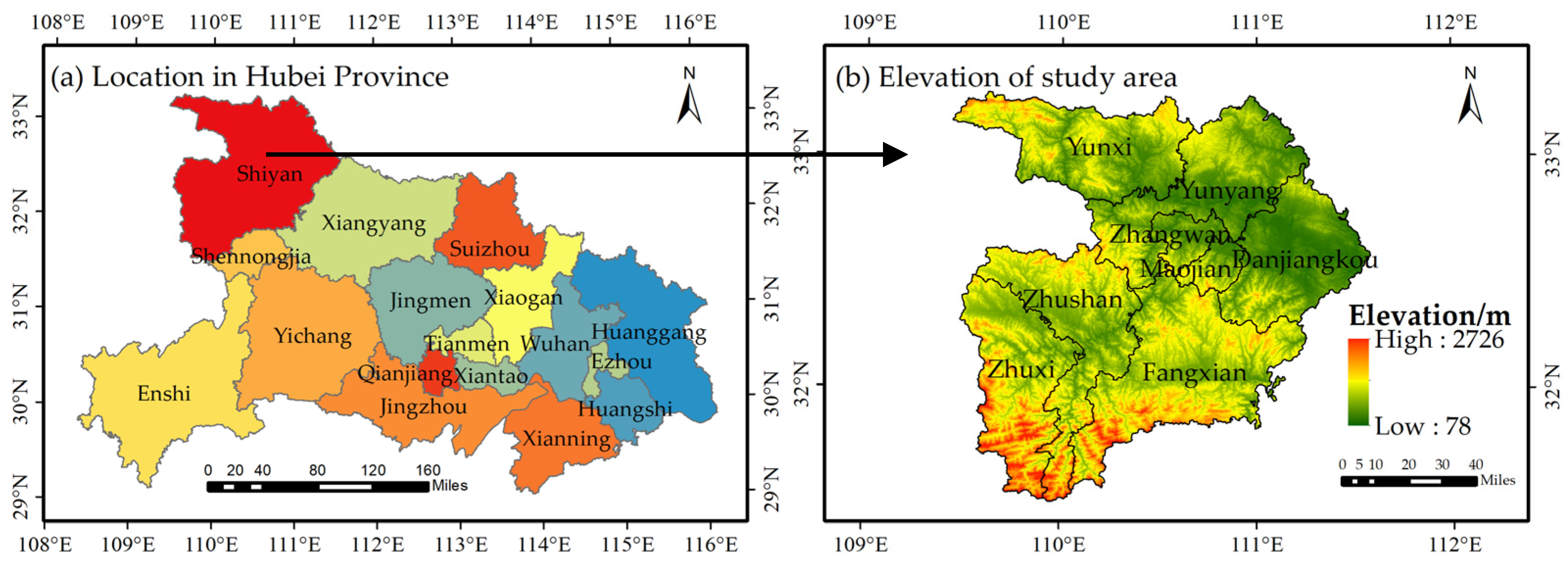
Article

Evolution of Habitat Quality and Its Topographic Gradient Effect in Northwest Hubei Province from 2000 to 2020 Based on the InVEST Model

1
Faculty of Urban and Environmental Sciences, Central China Normal University, Wuhan 430079, China
2
Key Laboratory for Geographical Process Analysis & Simulation in Hubei Province, Central China Normal University, Wuhan 430079, China
3
Land Science Research Center, Central China Normal University, Wuhan 430079, China
*
Author to whom correspondence should be addressed.
Land 2021, 10(8), 857; https://doi.org/10.3390/land10080857
Submission received: 6 July 2021 / Revised: 6 August 2021 / Accepted: 12 August 2021 / Published: 16 August 2021

Abstract

:
Regional land use change and ecological security are important fields and have been popular issues in global change research in recent years. Regional habitat quality is also an important embodiment of the service function and health of ecosystems. Taking Shiyan City of Hubei Province as an example, the spatiotemporal differences in habitat quality in Shiyan City were evaluated using the habitat quality module of the InVEST model and GIS spatial analysis method based on DEM and land use data from 2000, 2005, 2010, 2015, and 2020. According to the habitat quality index values, the habitats were divided into four levels indicating habitat quality: I (very bad), II (bad), III (good), and IV (excellent), and the topographic gradient effect of habitat quality was studied using the topographic position index. The results show the following. (1) The habitat quality of Shiyan City showed relatively high and obvious spatial heterogeneity overall and, more specifically, was high in the northwest and southwest, moderate in the center, and low in the northeast. The higher quality habitats (levels III, IV) were mainly distributed in mountain and hill areas and water areas, while those with lower quality habitats (levels I, II) were mainly distributed in agricultural urban areas. (2) From 2000 to 2020, the overall average habitat quality of Shiyan City first increased, then decreased, and then increased again. Additionally, the habitat area increased with an improvement in the level. There was a trend in habitat transformation moving from low to high quality level, showing a spatial pattern of “rising in the southwest and falling in the northeast”. (3) The habitat quality in the water area and woodland area was the highest, followed by grassland, and that of cultivated land was the lowest. From 2000 to 2020, the habitat quality of cultivated land, woodland, and grassland decreased slightly, while the habitat quality of water increased significantly. (4) The higher the level of the topographic position index, the smaller the change range of land use types with time. The terrain gradient effect of habitat quality was significant. With the increase in terrain level, the average habitat quality correspondingly improved, but the increasing range became smaller and smaller. These results are helpful in revealing the spatiotemporal evolution of habitat quality caused by land use changes in Shiyan City and can provide a scientific basis for the optimization of regional ecosystem patterns and land use planning and management, and they are of great significance for planning the rational and sustainable use of land resources and the construction of an ecological civilization.

1. Introduction

Habitat quality refers to the ability of an ecosystem to provide suitable and sustainable living conditions for individuals and populations [1], which is an important reflection of regional biodiversity and ecosystem functioning [2]. The quality of a habitat is decisive in the sustainable and harmonious development of human beings, nature, and other species [3]. The early methods for habitat quality assessment involve obtaining parameters related to the habitat quality in the study area through field surveys to construct an evaluation index system and to use certain mathematical methods for the comprehensive evaluation of habitat quality. For example, Ma Mingdong et al. [4] investigated and evaluated the multi-factor quantitative habitat quality of spruce natural stand; Liu Minxia [5] investigated and evaluated the biodiversity characteristics and habitat quality of Dunhuang West Lake Nature Reserve; Wang Jianhua et al. [6] investigated and evaluated the habitat quality of the river in Naoli River Basin; and Liu Hua et al. [7] investigated and evaluated the habitat quality of Yixing River in Taihu Lake Basin. Methods based on field survey sampling to evaluate habitat quality have great limitations. For example, field sampling tends to serve a specific target on a small scale and has high requirements for labor, material resources, and time. It is operationally and relatively difficult, and conducting long-term data analysis is also challenging, with evaluation results being difficult to promote and compare.
In recent years, the combination of 3S and habitat assessment has bypassed the limitations of early methods, making it possible to conduct quantitative, visual, and fine-scale analysis and assessment of the large and medium-scale changes in biodiversity, considering both spatiotemporal scales. At the same time, ecological models are constantly being updated and improved, and the effects as determined by spatial change analysis and simulation of habitat quality are becoming increasingly obvious, with examples such as the InVEST model habitat quality assessment module [8], the biodiversity evaluation module in IDRISI software [9], the SoLVES model [10,11], the HIS model [12], etc. Among these, the habitat quality module in the InVEST model is designed to establish the relationship between different land use types and threat sources, using data for land use types in the study area and combining the habitat suitability, habitat sensitivity, and threat intensity of disturbance factors of each ecosystem type to assess habitat quality distribution and degradation. This model is widely used because the required parameters can be conveniently acquired with low application cost, high evaluation accuracy, and strong spatial analysis function [13]. For example, using the InVEST model, Zhou Liang et al. [14] studied the impact of urban expansion on habitat quality in the densely populated areas of the Loess Plateau from 1990 to 2018; Wang Geng et al. [15] studied the impact of land use change on habitat quality in the coastal areas of Dandong from 2000 to 2018; Zhou Ting et al. [16] studied the spatial relationship between human activities and habitat quality in the Shennongjia forest region from 1995 to 2015; Wang Jun et al. [17] analyzed the spatiotemporal variation characteristics of habitat quality in the Minjiang River Basin from 2000 to 2040.
The results of former research demonstrate that the InVEST model has characteristics that make it suitable for different regional scales and shows better integration of ecological processes and good spatial display effects, and the rationality of the model has been well verified. In recent years, research has focused on the distribution of topographic factors and land use types, regional habitat quality status, and the spatiotemporal variation characteristics of habitat quality. Few scholars have paid attention to the topographic gradient effect of habitat quality, and there is few research involving the effects of topographic factors on the spatial heterogeneity of habitat quality. The terrain is often an important factor that affects the ecological structure and spatial pattern differentiation of mountainous areas [18] and the spatial distribution of landscape patterns and ecosystem services [19] and has an important impact on the material exchange and energy cycle of the habitat system. Strengthening the research on habitat quality and topographic gradient effects is helpful for establishing a topographic information map of habitat quality, which is of great significance for comprehensively and deeply understanding the spatiotemporal differentiation characteristics of habitat quality.
Shiyan City, Hubei Province, has a vast territory characterized by complex terrain that can be divided into four main landform types of hills, low mountains, middle mountains, and high mountains and two secondary landform types of valley flats and intermountain basins. The mountain ranges are characterized by large mountains, narrow valleys, large elevation differences, large slopes, and deep cuts, which are suitable for topographic-scale research. The unbalanced distribution of population, resources, and the environment has become the main obstacle to the sustainable development of cities. Considering this, this study takes Shiyan City as the research object. Based on the land use data from 2000, 2005, 2010, 2015, and 2020, the habitat quality module in the InVEST model was used to evaluate the regional habitat quality and to analyze the spatiotemporal aspects of the habitat quality from the grid scale. In addition, this study also uses DEM (digital elevation model) data, the topographic position index, and GIS spatial analysis methods to study the terrain gradient effect of habitat quality at the county scale in order to enrich the theoretical research on habitat quality change in Shiyan City. The results are expected to serve as a reference for biodiversity protection, land use planning, ecological security pattern construction, and spatial optimization in Shiyan City, as well as to promote the construction of an ecological civilization.

2. Materials and Methods

2.1. Study Area

Shiyan City is located in the northwest of Hubei Province (Figure 1) in the eastern part of the Qinba Mountains and the upper and middle reaches of the Hanjiang River, and it borders three provinces and cities, including western Henan, southern Shanxi, and eastern Chongqing. Shiyan City spans 31°30′ N to 33°16′ N, 109°29′ E to 111°16′ E and has jurisdiction over 8 county-level administrative districts, including 3 municipal districts, 1 county-level city, and 4 counties. It is about 200 km from east to west and about 195.5 km from north to south, with a land area of 23,680 square km. The city has a permanent population of 3.209 million. The city terrain is characterized by high elevation in the north and south with low elevation in in the center and slopes from southwest to northeast. The city terrain can be divided into four main landform types of hills, low mountains, middle mountains, and high mountains and two secondary landform types of river valley flats and intermountain basins. The highest point in Shiyan City, Zhuxi Congping, is 2740.2 m above sea level, while the lowest point, Danjiangkou Panjiayan, is 87 m above sea level. The city has a subtropical monsoon climate with an average annual precipitation of 834 mm and an average temperature of 15.2 °C. Shiyan City has large and steep mountains, vertical and horizontal rivers, large drops, and rapid water flow. It is rich in biological, mineral, and water resources.
Shiyan is an emerging modern city, with Xiangyu railway providing transportation to all parts of the country, national highways 209 and 316 connecting east, west, north, and south, and an expressway to Wuhan, Xi’an, and Baoji. People travel in all directions. The automobile, hydropower, tourism, and ecological industries have become the four pillar industries of Shiyan’s economic development. By the end of 2020, Shiyan had basically completed the goals and tasks of the “13th Five-Year Plan”, making decisive achievements in building a moderately prosperous society in an all-round way. It is expected to achieve a regional GDP of 195 billion yuan and a per capita GDP close to 60,000 yuan. In the process of social and economic development of Shiyan City, the imbalance in spatial allocation of population, resources, and environment has brought about many ecological problems that cause the landscape pattern and ecological environment of Shiyan City to constantly change. Natural landscapes have gradually been replaced by artificial buildings. The land area available for cultivation is continuously being reduced while the area corresponding to built-up land is increasing. The regional habitat is being further divided, with the degree of habitat fragmentation increasing, and the discordance between man and land is becoming increasingly prominent. Human activities have not only caused the degradation of biological resources but have also resulted in a series of environmental issues. The overloading of ecological carrying capacity in certain areas has threatened the ecological security of Shiyan, and this has become the main obstacle to realizing the sustainable development of the city. The task of ecological environmental protection is still under pressure and there is a long way to go in achieving this.

2.2. Data Resources and Preparation

The land use data from 2000, 2005, 2010, 2015, and 2020 in this study are from the Resource and Environmental Science and Data Center of the Chinese Academy of Sciences (http://www.resdc.cn (accessed on 15 April 2021)). The US satellite Landsat-TM/ETM and Landsat 8 multispectral images are the information sources for these data. Based on the high-resolution remote sensing ground survey observation technology, the data are constructed by a human–computer interactive visual interpretation. The spatial resolution is 30 m, and the classification accuracy is over 85%. The remote sensing images in central China were acquired in early March or late October. The data series integrate the land use types of the research area based on 6 first-class categories of cultivated land, woodland, grassland, water, built-up land, and unused land, depending on the land resources and their use attributes. The second class includes division into 25 types according to the natural properties of land resources (Table 1), although only 18 of these secondary land types were observed in Shiyan.
The vector data of the basic geographic information administrative region boundaries, lakes and rivers, main roads, and main railways were derived from the national basic geographic database of 1:250,000 and 1:1,000,000 provided by the National Catalogue Service for Geographic Information (https://www.webmap.cn (accessed on 15 April 2021)). The DEM data is from NASA EARTHDATA (https://earthdata.nasa.gov (accessed on 15 April 2021)), the ASTER Global Digital Elevation Model V003 data were selected, and the spatial resolution of the data is 30 m.
This research was based on the ArcGIS 10.2 software platform to preprocess and analyze the related vector and raster data. The habitat quality of Shiyan was simulated based on the InVEST 3.9.0 model.

2.3. Habitat Quality Assessment

2.3.1. Habitat Quality Module of the InVEST Model

The InVEST model (Integrated Valuation of Ecosystem Services and Tradeoffs) was jointly developed by Stanford University, The Nature Conservancy, and the World Wildlife Fund in 2007 [25] and has been widely used in ecosystem service assessments [26]. By integrating RS and GIS technology, the model simulates the dynamic change process of ecosystem service function according to the change in land use and cover type and realizes spatial visualization of the quantitative evaluation of ecosystem service value. The habitat quality module of the InVEST model aims to establish the relationship between different land use types and threat sources. Based on the data of land use types in the study area combined with the habitat suitability of animals and plants, habitat sensitivity, and threat intensity of disturbance factors of each ecosystem type, the habitat quality index can be calculated based on two aspects: the natural attributes of the habitat and the degree of habitat degradation caused by external threats [27,28]. The module reflects the influence of people’s production and life on the surrounding environment [29]. The greater the severity of activities, the greater the stress to the environment, and the lower its quality and level of biological diversity [29]. In contrast, the better the habitat quality, the less the area is disturbed by human activities, and the higher the level of biodiversity [30]. The advantage of this method is that it can replace the detailed investigation method as well as allow quantitative monitoring of the change in habitat quality within a short time scale. The spatial attenuation of threats can be described by linear or exponential distance attenuation functions. The calculation formula of the stress level i r x y of the threat factor r in the grid y to the habitat grid x is as follows:
i r x y = 1 ( d x y d r m a x )   ( linear   decay )
i r x y = e x p ( ( 2.99 d r m a x ) )   ( exponential   decay )
where d x y is the linear distance between grid x and grid y , and d r m a x is the maximum impact distance of threat factor r on the habitat. The total threat level D x j of grid cell x in habitat type j can be expressed as
D x j = r = 1 R y = 1 Y r ( w r r = 1 R w r ) r y i r x y β x S j r
where R is the number of threat factors, w r is the weight of the threat factor r with a value of 0–1, indicating the relative destructive power of the stress factor to all habitats, Y r is the total number of grid cells of the threat factor r in land use map, r y is the number of stress factors on each grid in the land use map, and S j r is the relative sensitivity of land use type j to threat factor r with a value of 0–1. The closer the value is to 1, the greater the relative sensitivity; β x is the legal accessibility of the grid unit x , which refers to the protection degree of land resources or ecosystems under the current policies, laws, regulations, and regulations and their implementation methods—that is, the accessibility level of various threat factors to grid x . The value range is 0–1, and the closer the value is to 1, the easier it is for the threat to reach the grid. This paper temporarily ignores the specific land protection areas in Shiyan City and considers that all land cover types in the study area are equally and uniformly protected by national laws and regulations, and the system will automatically assign a value of 1, which corresponds to safe arrival.
The habitat quality index is calculated using the following formula:
Q x j = H j ( 1 ( D x j z D x j z + K z ) )
where Q x j is the habitat quality index of grid x in land use type j , and its value is between 0 and 1. The higher the value, the better the habitat quality. H j is the habitat suitability of land use type j , and its value range is 0–1, in which 1 indicates most suitable. K is a half-saturation constant, generally taken as 1/2 of the maximum value of the habitat degradation degree D x j . The z value is the default parameter and is a normalized constant whose value is usually set as 2.5.

2.3.2. Habitat Quality Module Parameter Setting

The measurement of habitat quality in the InVEST model includes four elements: the relative weight of the impact of each threat factor, the relative sensitivity of each habitat to each threat factor, the distance between the habitat and the threat source, and the accessibility of the habitat. The threat sensitivity of habitat quality in this model should be determined according to the common rules of biodiversity conservation [31,32]. According to previous experience, stress factors related to human production and life have the greatest influence on the surrounding environment. The cultivated land and built-up land have intense human activities and extremely low biodiversity. Unused land is essentially without vegetation cover, and the ecological environment is harsh, which has an erosive effect on the external habitat and will affect the stability of the surrounding ecological environment. The higher the intensity of human activities, the greater the impact on the biodiversity of the surrounding habitat. The greater the sensitivity, the worse the anti-interference ability of habitat types to threat factors is. Therefore, we collected data from relevant examples of existing studies in many regions [33], and analyzed the types, weights, and habitat sensitivity assignment of the threat sources in the literature. Referring to the user guide manual of the InVEST model and the expert opinions of the region and considering the special geographical environment of the study area, we selected eight types of threat sources, namely paddy field, dry land, urban land, rural residential land, other construction land, unused land, main railways, and main roads. Additionally, the values of habitat threat sources and related parameters (Table 2), the habitat suitability of each land use type and its sensitivity to different threat sources were evaluated (Table 3).
The InVEST model uses the habitat quality index to reflect the status of regional habitat quality. The habitat quality index in the model varied continuously from 0 to 1 at the grid level. The larger the value, the better the habitat quality; the more complete the structure and function of the corresponding ecological environment, the more conducive it is to the maintenance of biodiversity. The smaller the value, the worse the habitat quality; the more imperfect the structure and function of the ecological environment, the more unfavorable it is to the maintenance of biodiversity, and the more vulnerable the ecological environment is to external disturbance and destruction.

2.4. Terrain Index

The topography of Shiyan City is complex, and topographical conditions have greater constraints on the spatial pattern of land use and the spatial distribution of habitat quality. Therefore, this study uses the topographic position index to measure the topographic gradient. The terrain index is a composite index used to analyze the elevation and slope attribute information of any point in space, which can comprehensively reflect the spatial differentiation of topographical conditions [34]. The formula is as follows:
T = lg [ ( E E ¯ + 1 ) × ( S S ¯ + 1 ) ]
In the formula, T is the topographic position index, E and E ¯ refer to the elevation value (m) and average elevation value (m) of any grid in the space, respectively, S and S ¯ refer to the slope value (°) and average slope value (°) of any grid in the space, respectively. Generally, the value for grid topographic position index is larger when there is both high elevation and slope value, while the value for grid topographic position index is lower when there is both low elevation and slope value, and with high elevation and low slope value or with low elevation and high slope value, the value for grid topographic position index is moderate.

3. Results and Analyses

3.1. Land Use Change Characteristics

According to the five land use maps of Shiyan City from 2000, 2005, 2010, 2015, and 2020 (Figure 2), the proportion of area for each land use type in the five periods (Figure 3) and the change in land use type in the different periods (Figure 4) were obtained. The main land use types in Shiyan are woodland, cultivated land, and grassland, which account for about 97% of the total area of Shiyan. The area proportion of each land use type in the five phases of the study area remained stable, but all changed to different degrees. In general, from 2000 to 2020, the increase in proportion of built-up land area was 282.68%, the increase in proportion of water areas was 18.01%, the decrease in proportion of unused land area was 12.56%, the change in other types of areas was small, and the decrease in proportion of cultivated land, grassland, and woodland area was 2.52%, 1.81%, and 0.65%, respectively. The decrease in the area of the natural landscape dominated by woodland and grassland and the increase in the area of cultural landscapes dominated by built-up land reflect the increasing disturbance from human activities in this area. From 2000 to 2005, the increased proportion of built-up land area was 6.40%, water area was 5.17%, and the change in other types of areas was small. From 2005 to 2010, the increase in proportion of built-up land area was 99.95%, the increase in proportion of water area was 16.66%, the increase in proportion of unused land area was 14.40%, and the change in other types of areas was small. From 2010 to 2015, the increase in proportion of built-up land area was 110.26%, the increase in proportion of water area was 9.87%, the decrease in proportion of unused land area was 15.05%, and the change in other types of areas was small. From 2015 to 2020, the reduction in proportion of built-up land area was 14.45%, the reduction in proportion of water area was 12.46%, the reduction in proportion of unused land area was 11.07%, and the change in other types of areas was small.

3.2. Spatiotemporal Variation Characteristics of Habitat Quality

By running the habitat quality module of InVEST, the spatial distribution maps of habitat quality in Shiyan in 2000, 2005, 2010, 2015, and 2020 were obtained. On the grid layer, the habitat quality index is a value that varies continuously from 0 to 1. The closer the value is to 1, the better the habitat quality. The habitat is relatively complete and has a corresponding structure and function, which is conducive to maintaining biodiversity. In order to describe the evolution law of habitat quality in the study area more accurately, the habitat quality was divided into four levels using the natural breakpoint method in ArcGIS, namely I (very bad), II (bad), III (good), and IV (excellent), and the corresponding habitat quality index value ranges were 0.0–0.4, 0.4–0.6, 0.6–0.8, and 0.8–1.0, respectively.
In terms of spatial distribution (Figure 5), the habitat quality of the entire city was high in the northwest and southwest, moderate in the center, and low in the northeast. The distribution of habitat quality was consistent with that of land use types. The habitat quality was higher in woodland and grassland, but lower in cultivated land and built-up land. From 2000 to 2020, the habitat quality of Shiyan City showed obvious spatial heterogeneity. Due to the large proportion of woodland in the study area, the higher quality habitats (III and IV) were widely distributed, with an average area proportion of about 61% in the five periods. The distribution characteristics of these habitats were different. Habitats of quality level IV were mainly distributed in the southwest of Zhuxi County, the southeast of Fangxian County, and the mountainous and hilly areas in the southeast of Danjiangkou City. Habitats of level III were mainly distributed in the southwest of Fangxian County, the west of Yunyang District, the south of Zhangwan District, and the center of Maojian District in the mountainous and hilly areas. Due to having low population density, less human disturbance, a large number of woodland and grassland areas, relatively high species richness, high vegetation coverage and good natural ecological conditions, and a number of ecological protection policies in place, the mountain and hilly areas have become a habitat for many types of birds, insects, and other organisms due to their high habitat quality and relative stability. In addition, the habitat quality of Hanjiang River and Duhe River was also at a high level, benefiting from rich water resources and being suitable for the survival of aquatic animals and plants. Habitats of level II were mainly distributed in the hills and peaceful lands in the south of Yunxi County and the east of Yunyang District. The land use structure in these areas was mainly sparse woodland and medium coverage grassland with low vegetation coverage, a single ecosystem type, low biodiversity, and a fragile ecological environment. Habitats of level I were mainly distributed in the agricultural production areas in the north of Zhuxi County, the center of Fangxian County, and the center of Danjiangkou City. The land use structure in these areas was mainly dry land, paddy fields, and urban land. The population density was large, human activity was high, the vegetation coverage was low, the original natural environment had been transformed, the biodiversity was low [35], and the ecological environment was relatively fragile; it was not suitable for living organisms. Therefore, the spatial distribution of habitat quality is strongly correlated with topography and resource endowment.
From the time scale data (Table 4), it was found that the habitat area increased with an improvement in the level of habitat quality. According to the statistics from the area ratio of each level of habitat, the proportion of level IV habitats was the highest, at about 36%, and the proportion of level III and IV habitats was 61%, which indicated that the overall habitat quality of Shiyan City was at a high level. In 2000, 2005, 2010, 2015, and 2020, the overall average habitat quality index values for Shiyan City were 0.7217, 0.7221, 0.7192, 0.7157, and 0.7181, respectively. The habitat quality first increased, then decreased, and then increased again. From 2000 to 2020, the habitat quality decreased by 0.50%, and the area proportion of each habitat showed little change. The area proportion of level II habitats decreased gradually from 22.68% to 22.23%, while the area proportion of IV increased gradually from 35.89% to 36.33%. The increase and decrease degree were essentially the same, reflecting the trend of the transformation from low to high habitat quality. While the area of built-up land in Shiyan City increased rapidly from 2005 to 2015, the woodland, grassland, and farmland were occupied, the habitat was continuously divided, there was an aggravation in the degree of habitat fragmentation, connectivity worsened, and the overall average habitat quality continued to decline. The habitat in Shiyan City gradually recovered from 2015 to 2020. The promotion of policies and development of concepts such as returning farmland to forest or grassland, ecological civilization construction, clear water and green mountains becoming gold and silver mountains, as well as the implementation of measures such as energy conservation, emission reduction, and environmental protection led to an improvement in the average habitat quality.
According to statistics from the habitat quality changes in Shiyan City from 2000 to 2020 (Figure 6), the change in habitat quality index in Danjiangkou, Fangxian, Yunxi, Yunyang, Zhushan, and Zhuxi counties varied. Additionally, the decrease in the habitat quality index values of Maojian and Zhangwan districts was in the range of 0.03–0.04. Among them, the habitat quality index of Maojian District decreased the most from 0.73 to 0.69, followed by the habitat quality index in Zhangwan District from 0.74 to 0.71, which was mainly due to the increase in built-up land, which more greatly threatened the habitat more and resulted in the decrease in habitat quality.
In order to establish spatial visualization of the dynamic increase and decrease in habitat quality in Shiyan City from 2000 to 2020 and to further explore the spatial differentiation characteristics of habitat quality, the grid calculator tool of the ArcGIS 10.2 platform was used to calculate the difference in the habitat quality Shiyan City in 2000, 2005, 2010, 2015, and 2020 as a distribution map. Additionally, the natural breakpoint method was also used to classify the changes according to five levels: rapid decline, decline, no obvious change, promotion, and rapid promotion (Figure 7). As can be seen from the figure, the habitat quality in most areas of Shiyan City showed no significant change from 2000 to 2020, and the overall spatial pattern was “rising in the southwest to falling in the northeast”. From 2000 to 2010, the areas showing habitat quality improvement were mainly located in the Hanjiang River of Yunyang District and the Hanjiang River of Danjiangkou City. The land use structure of these places was mostly water area, and the increase in water surface caused the habitat quality to improve. From 2005 to 2010, the areas of declining habitat quality were mainly located in the southern part of Yunyang District, the northern part of Zhangwan District, and the northern part of Maojian District. The land use structure of these areas was mostly built-up land, and the increase in construction land was the main threat to habitat quality change. From 2010 to 2015, habitat quality improvement areas were mainly located in Duhe River in Zhushan County and Huiwan River in Zhuxi County. The areas of declining habitat quality were mainly located in the central part of Yunyang District, the eastern part of Zhangwan District, and the northern part of Maojian District. There is urgent demand for economic development in Shiyan City. With the intensification of urbanization, the proportion of construction land has increased rapidly and has occupied the bare land and cultivated land. As a result, the surrounding habitats have been squeezed and divided, leading to the gradual expansion of areas with low habitat quality to the surrounding areas and a successive decrease in the regional habitat quality. At the same time, a series of pollutants discharged in the process of construction and production may cause the degradation of nearby habitats, destroy and disturb the recreational environment of surrounding species, and pose a greater threat to the maintenance of biodiversity. From 2015 to 2020, the area of habitat quality improvement was mainly located in the south of Yunyang District, the north of Maojian District, and the forestland in the northwest and northeast of Zhangwan District. The main reason was that the vegetation coverage rate increased due to the conversion of farmland to forest and afforestation. The degradation of habitat quality was mainly located in the central part of Yunyang District and the central part of Danjiangkou City. The continuous enhancement of the social economy and human activities has detrimentally affected habitat quality.

3.3. Habitat Quality Change Characteristics of Different Land Types

Regional habitat quality is greatly affected by land use, and land use change causes changes in habitat quality, which may lead to the deepening of habitat fragmentation [36]. Land use change contains a large amount of information corresponding to human activities, which affects the quality of the landscape ecological environment by interfering with landscape types and spatial patterns [37,38], leading to a series of changes in the composition of the ecosystem and, consequently, changes in biodiversity, affecting the relationship between land use and the ecosystem. In order to understand the impact of land use changes on habitat quality, the distribution and average habitat quality of different land use types in 2000, 2005, 2010, 2015, and 2020 in Shiyan City were statistically analyzed. The habitat quality of different land use types did not fluctuate significantly in the five studied periods (Table 5 and Figure 8). The average habitat quality of water, woodland, and grassland was 0.9265, 0.8114, and 0.6391, respectively. Additionally, the habitat quality was relatively high. The average habitat quality of cultivated land was 0.3319, which was relatively low. The distribution of habitat quality was generally consistent with that of land use types. The quality of the dominant habitats in cultivated land, woodland, grassland, and water were classified as level I, IV, II, and IV, respectively. Correspondingly, the habitat quality of water and woodland was the highest, followed by grassland, and the habitat quality of cultivated land was the lowest. From 2000 to 2020, the area of cultivated land, woodland, and grassland decreased. Due to the influence of human disturbance, the habitats showed different degrees of degradation, leading to a slight decline in habitat quality and with a small range of decline of 0.0006, 0.0007, and 0.0003, respectively. The water area increased, and the habitat quality greatly improved by 0.0293. From 2005 to 2015, the area of cultivated land, woodland, and grassland decreased continuously, and the area of built-up land, as a source of threat, increased. The high habitat quality of cultivated land, woodland, and grassland continued to degrade to lower habitat quality. This is because, with the intensification of urbanization, urban expansion transformed the cultivated land, woodland, grassland, and other habitats in the suburbs into built-up land. In addition, human activities, such as deforestation and land destruction, have transformed the original habitat into a threat factor, which has a great impact on regional biodiversity, including the cutting off of spatial connectivity [39], and this further aggravated the degree of the threat. From 2000 to 2015, the area for water continued to increase, and its habitat quality also continued to improve, showing the most significant improvement in habitat quality of all land types. In conclusion, woodland and water areas contributed the most to the habitat quality of Shiyan City, and the degradation of woodland was the main reason for the decline in regional habitat quality.

3.4. Topographic Gradient Effect of Habitat Quality

3.4.1. Topographic Features of Shiyan City

Using ArcGIS software to extract slope and elevation data based on DEM data, we calculated the topographic position index values for Shiyan City according to Formula (5). The resulting values were in the range of 0.0491–1.2074. The natural breakpoint method was used to classify these values according to five levels (Figure 9): I (<0.33), II (0.33–0.50), III (0.50–0.64), IV (0.64–0.78), and V (0.78–1.21). It can be seen from Figure 9 that the topography of Shiyan City is low in the center, high in the south and north, and slopes from the southwest to the northeast. The topographic position index can fully describe the distribution of the regional topography. The highest point in Shiyan City, Zhuxi Congping, is 2740.2 m above sea level, while the lowest point, Danjiangkou Panjiayan, is 87 m above sea level. As can be seen from Figure 10, the topographic locations in the study area are mainly at level III, accounting for more than 29%, followed by levels II, IV, and V, which account for 22.39%, 24.36%, and 12.81%, respectively. The topographic locations at level I are the least, accounting for only 10.78%.

3.4.2. Topographic Gradient Effect of Land Use

The terrain of Shiyan City is relatively complex, and the intensity of human activities and the vertical differentiation of the climate result in the land use structure having obvious terrain gradient effects, which restrict the distribution of land use types to a certain extent. Combined with the classification of the topographic position index of Shiyan City, the reclassified raster map of the topographic position index was superimposed with the corresponding land use map of 2000, 2005, 2010, 2015, and 2020 in ArcGIS to obtain the land use change of each topographic position index level (Table 6 and Figure 11). It can be seen from the chart that the main land use types in Shiyan City are woodland and cultivated land. The land use types corresponding to topographic position index levels from I to V were mainly woodland. With the increase in the topographic level, the proportion of cultivated land, grassland, waters, built-up land, and unused land showed a decreasing trend, while the proportion of woodland increased significantly. From 2000 to 2020, the proportion of cultivated land, woodland, and grassland corresponding to each topographic position index level showed a decreasing trend, while the proportion of waters and built-up land increased, and the proportion of unused land remained essentially unchanged. Moreover, the higher the level of topographic position index, the smaller the variation range of each land use type over time. This is because the flatter the terrain, the greater the intensity of human activities, and the more intense the disturbance of human factors on land use. While severe climate, natural disasters, and other factors have a greater impact on land use change in high-lying areas, compared to natural factors, human factors have a more significant impact on land use in the short term.

3.4.3. Topographic Gradient Effect of Habitat Quality

Topography is an important factor that affects the distribution pattern of populations and maintains community diversity [40]. The topography of Shiyan City is relatively complex, and the spatial distribution of its habitat quality will be affected by the topography to a large extent. Since the intensity of human activities is usually relatively consistent within the administrative regions and the establishment and implementation of ecological policies are all based on the county as the minimum unit [41], the terrain index and habitat quality of each county in Shiyan City are calculated, and the topographic gradient effect of habitat quality is studied with the county as the basic unit (Figure 12). It can be seen from the figure that the topographic position index of Danjiangkou City, Yunyang District, and Zhangwan District was 0.40, 0.49 and 0.49, respectively, which was at level II, with an average habitat quality of 0.69, 0.69, and 0.72, respectively. The topographic position index of Maojian District, Yunxi County, and Zhushan County was 0.55, 0.59 and 0.62, respectively, which was at level III, and the average habitat quality in the five stages was 0.70, 0.75, and 0.70, respectively. The topographic position index of Fangxian and Zhuxi County was 0.64 and 0.68, respectively, which was at level IV, and the average habitat quality in the five phases was 0.74 and 0.75, respectively. The counties with higher topographic position index level generally have higher average habitat quality in the five stages.
By using ArcGIS software, the average habitat quality and distribution of different habitat quality levels on the topographic position index levels of Shiyan City from 2000 to 2020 were obtained by superposition analysis of habitat quality and terrain gradient (Table 7 and Figure 13). The distribution characteristics of habitat quality with the change of terrain gradient were discussed, and the impact of terrain change on the spatial pattern of habitat quality was revealed. The results show that the spatial distribution of habitat quality at different levels was significantly different on the topographic gradient. The increases in the topographic position index level led to the average habitat quality being improved. With the increase in the gradient, the impact of human disturbance was reduced and the vegetation coverage was higher. However, the increase in the average habitat quality gradually diminished, showing a relatively obvious geographical hierarchical distribution characteristic. In 2020, the average habitat quality of topographic position index level V was 1.33 times that of level I, and the increase rates between topographic position index level I and level V were 10.48%, 10.02%, 5.70%, and 3.74%, respectively, indicating that the topographic gradient effect of habitat quality was more significant when the terrain was relatively gentle. From 2000 to 2020, the habitat quality of each level of terrain showed a downward trend, with successive change values of −0.0098, −0.0074, −0.0020, −0.0011, and −0.0007. The reason is that the quantity of forest and grassland continued to decrease, leading to the general decline in habitat quality. The topography of the study area plays an important role in the spatial distribution pattern of habitat quality. The reason is that the difference in the geomorphic morphology will lead to different effects of human activities on land use in space [42,43], which will lead to different habitat qualities in the spatial distribution. Therefore, the influence of topography should be fully considered in the optimization of the ecosystem pattern and land use planning and management in the study area.

4. Discussion

In this study, the habitat quality module of the InVEST model was used to evaluate the change in the pattern of habitat quality in Shiyan City from 2000 to 2020, revealing the spatiotemporal variation characteristics of habitat quality in the process of land use change and analyzing the distribution characteristics of habitat quality from a topographic perspective. The results may provide a scientific basis for the optimization of regional ecosystem pattern and land use planning and management, which is of great significance for the rational and sustainable use of land resources and the construction of an ecological civilization [44].
The study found that the habitat quality in Shiyan City showed obvious spatial heterogeneity. The higher quality habitats (III, IV) were mainly distributed in the mountainous and hilly areas, lakes, and rivers, while the lower quality habitats (I, II) were mainly distributed in the agricultural urban areas, which was consistent with the results of Wang Geng et al. [15] and Xie Yuchu et al. [30]. This was because the habitat quality was correlated with topography and land cover to a certain extent. The mountainous and hilly areas had low population density, less human disturbance, a large number of woodland and grassland areas, relatively high species richness, high vegetation coverage, and good natural ecological conditions. Rich water resources were suitable for the survival of aquatic animals and plants. Therefore, we should pay more attention to water resources and effectively limit the encroachment and pollution of cultivated land and built-up land on water. The agricultural urban areas had large population density, strong interference from human activities, low vegetation coverage, low biodiversity, and a relatively fragile ecological environment. From 2000 to 2020, the overall spatial pattern of Shiyan City was “rising in the southwest to falling in the northeast”. The habitat quality was mainly improved in water and woodlands. The increase in water surface and the improvement to the vegetation coverage rate improved the habitat quality. The decrease in habitat quality was mainly caused by built-up land. Regional resource endowment will limit the overall level of habitat quality, while industrial development and land use will affect its change trend to a certain extent, resulting in the difference in the distribution and change level of habitat quality [45]. With the acceleration in the urbanization process, economic development, and population increases, the discordance between people and land is increasing. Urban expansion encroaches on original habitats, forming a new source of threat. As a result, the surrounding habitats have been squeezed and divided, leading to the successive decrease in the regional habitat quality. Therefore, we should strictly control the expansion of built-up land, improve optimization of the internal urban layout, minimize the scale of built-up land expansion to promote economic development, and limit the phenomenon of blind and uncontrolled urban expansion [46]. From 2000 to 2020, the habitat quality of all terrain levels showed a downward trend, and the number of forest and grasslands continued to decrease, leading to a general decline in habitat quality. Therefore, it is necessary to strengthen the control of the use of forestland, build and improve forest resource protection and restoration systems, and further prioritize the protection of forests and grassland ecology [47]. At the same time, attention should be paid to the protection of cultivated land, as its role in ensuring food security cannot be ignored. It is necessary to encourage the development of ecological agriculture and to reduce the use of chemical fertilizers and pesticides that threaten the survival of animals and plants. We must be alert to the destruction of habitats caused by economic development, strive to minimize human interference and, at the same time, continue to increase ecological restoration efforts to curb the trend of the declining function of biodiversity, in order to realize the optimal pattern of maximizing the comprehensive benefits of the society, economy, and ecology.
The InVEST model combines the advantages of RS and GIS and has characteristics that make it suitable for different regional scales and shows strong spatial analysis function and good spatial display effects. The results from this study alone are insufficient and need to be strengthened in the following respects. (1) The habitat quality in the InVEST model is an important reflection of regional biodiversity status. The model assumes that areas with good habitat quality have high biodiversity and that biodiversity will be affected when similar habitats are destroyed. While habitat destruction is one of the main causes of biodiversity loss [48], in practice, places with good habitat quality do not necessarily have high biodiversity. (2) While the InVEST model is relatively mature, it requires less data and has advantages in terms of spatial expression and dynamic research; the parameter setting in the calculation of the model is subjective to a certain extent, such as when considering the influence distance and weight of the threat factors. Additionally, habitat sensitivity and other parameters are not uniform. The results are difficult to compare horizontally. Further, parameter verification and rationality evaluation are worthy of further discussion. (3) The factors that affect the habitat quality are complex, and there is no in-depth analysis of the influence mechanism of each factor on its distribution formation. Moreover, the combined coercion effect of multiple threat sources may be far greater than the simple sum of the single threat source coercion effect. The InVEST model does not consider the combined coercion effect of threat sources. In the future, we could try to establish a more scientific, accurate, and unified parameter table. (4) The InVEST model integrates a variety of ecosystem service evaluation models, such as carbon storage, water conservation, soil conservation, etc., which can be used to analyze the changes in the comprehensive ecosystem services in Shiyan City in the future and may provide support for the protection of Shiyan’s ecological security [49,50,51,52,53,54,55,56,57].

5. Conclusions

In this study, DEM and five periods of land use grid data from 2000, 2005, 2010, 2015, and 2020 were used to evaluate the spatiotemporal variation characteristics of habitat quality in Shiyan City based on the InVEST model. Additionally, the topographic gradient effect of habitat quality was studied using the topographic position index. The following conclusions were reached:
(1)
From 2000 to 2020, the land use types in Shiyan City were mainly woodland, cultivated land, and grassland. The area of built-up land and waters increased by 282.68% and 18.01%, respectively. The proportion of unused land decreased by 12.56%, and the change in other types of areas was small;
(2)
The habitat quality in Shiyan City showed obvious spatial heterogeneity. The habitat quality of the whole city was high in the northwest and southwest, moderate in the center, and low in the northeast. Overall, the higher quality habitats (III, IV) were widely distributed;
(3)
From 2000 to 2020, the overall average habitat quality in Shiyan City first increased, then decreased, and then increased again. Further, the overall average habitat quality was at a higher level. The overall spatial pattern of Shiyan City was “rising in the southwest to falling in the northeast”;
(4)
The distribution of habitat quality was roughly consistent with that of the land use type. The highest habitat quality was found in water and woodland, followed by grassland, and the habitat quality of cultivated land was the lowest. From 2000 to 2020, the habitat quality of cultivated land, woodland, and grassland decreased slightly, while the habitat quality of water improved greatly;
(5)
The terrain level of Shiyan City is low in the center and high in the south and north. It slopes from southwest to northeast. The terrain level index of Shiyan City was mainly level III, followed by levels II, IV, and V, and level I was the least. The higher the level of topographic position index, the smaller the change of each land use type over time;
(6)
With the increase in the topographic position, the average habitat quality was improved correspondingly, but the increase gradually diminished. Additionally, the topographic gradient effect of habitat quality was more significant.

Author Contributions

Conceptualization, M.L., Y.Z. and P.X.; methodology, M.L.; software, M.L.; investigation, M.L.; writing—original draft preparation, M.L.; writing—review and editing, M.L., Y.T., H.H. and L.X.; supervision, Y.Z., P.X. and Y.T.; funding acquisition, Y.Z. All authors have read and agreed to the published version of the manuscript.

Funding

This research was funded by the National Natural Science Foundation of the People’s Republic of China project—Impact of land use evolution on watershed water resources and ecological response in the Jianghan Plain over 50 years (No. 41271534).

Institutional Review Board Statement

Not applicable.

Informed Consent Statement

Not applicable.

Data Availability Statement

No new data were created or analyzed in this study. Data sharing is not applicable to this article.

Conflicts of Interest

The authors declare no conflict of interest.

References

  1. Goldstein, J.H.; Caldarone, G.; Duarte, T.K.; Ennaanay, D.; Hannahs, N.; Mendoza, G.; Polasky, S.; Wolny, S.; Daily, G.C. Integrating ecosystem-service tradeoffs into land-use decisions. Proc. Natl. Acad. Sci. USA 2012, 109, 7565–7570. [Google Scholar] [CrossRef] [Green Version]
  2. Zhong, L.; Wang, J. Evaluation of the impact of land consolidation on habitat quality based on the InVEST model. Trans. Chin. Soc. Agric. Eng. 2017, 33, 250–255. [Google Scholar]
  3. Johnson, M.D. Measuring Habitat Quality: A Review. Condor 2007, 109, 489–504. [Google Scholar] [CrossRef]
  4. Ma, M.; Luo, C.; Zhang, J.; Hu, T.; Liu, Y. Multi-factor quantitative evaluation of habitat quality in natural spruce forests. Chin. J. Eco Agric. 2006, 2, 154–158. [Google Scholar]
  5. Liu, M. Biodiversity characteristics and habitat quality evaluation of Dunhuang West Lake Nature Reserve. Arid Land Resour. Environ. 2009, 23, 171–175. [Google Scholar]
  6. Wang, J.; Tian, J.; Lv, X. Evaluation of river habitat quality in Naoli River Basin. Acta Ecol. Sin. 2010, 30, 481–486. [Google Scholar]
  7. Liu, H.; Cai, Y.; Yu, M.; Gong, L.; An, S. Evaluation of River Habitat Quality in Yixing Area of Taihu Lake Basin. J. Ecol. 2012, 31, 1288–1295. [Google Scholar]
  8. Aneseyee, A.B.; Noszczyk, T.; Soromessa, T.; Elias, E. The InVEST Habitat Quality Model Associated with Land Use/Cover Changes: A Qualitative Case Study of the Winike Watershed in the Omo-Gibe Basin, Southwest Ethiopia. Remote Sens. 2020, 12, 1103. [Google Scholar] [CrossRef] [Green Version]
  9. Shanthala, D.B.S.; Murthy, M.S.R.; Bijan, D.; Jha, C.S. Identification of Potential Habitat Patches for Connectivity Using Weighted Linear Combination (WLC) and Integral Index of Connectivity (IIC) at East Godavari District, Andhra Pradesh, India. J. Indian Soc. Remote Sens. 2016, 44, 385–394. [Google Scholar] [CrossRef]
  10. Huo, S.; Huang, L.; Yan, L. Evaluation of Ecosystem Cultural Service Value Based on SolVES Model: Taking the Southern Ecological Park of Wuyi County, Zhejiang Province as an Example. Acta Ecol. Sin. 2018, 38, 3682–3691. [Google Scholar]
  11. Brown, G.; Brabyn, L. The extrapolation of social landscape values to a national level in New Zealand using landscape character classification. Appl. Geogr. 2012, 35, 84–94. [Google Scholar] [CrossRef]
  12. Wang, Z.; Chen, Z.; Hao, C. Evaluation of the suitability of red-crowned crane breeding habitat in Zhalong National Nature Reserve based on HSI model. Wetl. Sci. 2009, 7, 197–201. [Google Scholar]
  13. Huang, C.; Yang, J.; Zhang, W. Research progress of ecosystem service function assessment models. J. Ecol. 2013, 32, 3360–3367. [Google Scholar]
  14. Zhou, L.; Tang, J.; Liu, X.; Dang, X.; Mu, H. The impact of urban expansion on habitat quality in densely populated areas of the Loess Plateau: Taking Lanzhou, Xi’an-Xianyang and Taiyuan as examples. J. Appl. Ecol. 2021, 32, 261–270. [Google Scholar]
  15. Wang, G.; Wang, J. Study on the impact of land use change on habitat quality in the coastal area of Dandong. J. Ecol. Environ. 2021, 30, 621–630. [Google Scholar]
  16. Zhou, T.; Chen, W.; Li, J.; Liang, J. Research on the spatial relationship between human activities and habitat quality in Shennongjia forest area from 1995 to 2015. Acta Ecol. Sin. 2021, 15, 1–12. [Google Scholar]
  17. Wang, J.; Yan, Y.; Wang, J.; Ying, L.; Tang, Q. Study on the characteristics and prediction of temporal and spatial changes of habitat quality in the Minjiang River Basin. Acta Ecol. Sin. 2021, 14, 1–12. [Google Scholar]
  18. Sandro, P. Impact of Tourism on the Mountain Landscape of Central Italy; Elsevier: Amsterdam, The Netherlands, 1993; p. 24. [Google Scholar]
  19. Gong, W.; Wang, H.; Wang, X.; Fan, W.; Stott, P. Effect of terrain on landscape patterns and ecological effects by a gradient-based RS and GIS analysis. J. For. Res. 2017, 28, 1061–1072. [Google Scholar] [CrossRef]
  20. Li, H.; Wang, J.; Zhang, J.; Qin, F.; Hu, J.; Zhou, Z. Analysis of Characteristics and Driving Factors of Wetland Landscape Pattern Change in Henan Province from 1980 to 2015. Land 2021, 10, 564. [Google Scholar] [CrossRef]
  21. Wang, L.; Zheng, S.; Wang, X. The Spatiotemporal Changes and the Impacts of Climate Factors on Grassland in the Northern Songnen Plain (China). Sustainability 2021, 13, 6568. [Google Scholar] [CrossRef]
  22. Dong, S.; Cheng, H.; Li, Y.; Li, F.; Wang, Z.; Chen, F. Rural landscape types and recreational value spatial analysis of valley area of Loess Plateau: A case of Hulu Watershed, Gansu Province, China. Chin. Geogr. Sci. 2017, 27, 286–297. [Google Scholar] [CrossRef] [Green Version]
  23. Zhang, J.; Xu, W.; Qin, L.; Tian, Y. Spatial Distribution Estimates of the Urban Population Using DSM and DEM Data in China. ISPRS Int. J. Geo-Inf. 2018, 7, 435. [Google Scholar] [CrossRef] [Green Version]
  24. Li, J.; Sun, W.; Li, M.; Meng, L. Coupling coordination degree of production, living and ecological spaces and its influencing factors in the Yellow River Basin. J. Clean. Prod. 2021, 298, 126803. [Google Scholar] [CrossRef]
  25. Kareiva, P.; Tallis, H.; Ricketts, T.H.; Daily, G.C.; Polasky, S. Natural Capital: Theory and Practice of Mapping Ecosystem Services; Oxford University Press: Oxford, UK, 2011; p. 365. [Google Scholar]
  26. Tian, Y.; Huang, Y.; Zhang, Q.; Tao, J.; Zhang, Y.; Zhou, G.; Han, X.; Yang, Y.; Lin, J. Land cover and biodiversity simulation in Nanliujiang watershed of Beibu Gulf. China Environ. Sci. 2020, 40, 1320–1334. [Google Scholar]
  27. Nelson, E.; Mendoza, G.; Regetz, J.; Polasky, S.; Tallis, H.; Cameron, D.R.; Chan, K.M.A.; Daily, G.C.; Goldstein, J.; Kareiva, P.M.; et al. Modeling multiple ecosystem services, biodiversity conservation, commodity production, and tradeoffs at landscape scales. Front. Ecol. Environ. 2009, 7, 4–11. [Google Scholar] [CrossRef]
  28. Polasky, S.; Nelson, E.; Pennington, D.; Johnson, K.A. The Impact of Land-Use Change on Ecosystem Services, Biodiversity and Returns to Landowners: A Case Study in the State of Minnesota. Environ. Resour. Econ. 2011, 48, 219–242. [Google Scholar] [CrossRef]
  29. Zhang, C.; Fang, S. Identifying and Zoning Key Areas of Ecological Restoration for Territory in Resource-Based Cities: A Case Study of Huangshi City, China. Sustainability 2021, 13, 3931. [Google Scholar] [CrossRef]
  30. Xie, Y.; Gong, J.; Zhang, S.; Ma, X.; Hu, B. Research on the temporal and spatial pattern of landscape biodiversity in the Bailong River Basin based on remote sensing and InVEST model. Geogr. Sci. 2018, 38, 979–986. [Google Scholar]
  31. Terrado, M.; Sabater, S.; Chaplin-Kramer, B.; Mandle, L.; Ziv, G.; Acuña, V. Model development for the assessment of terrestrial and aquatic habitat quality in conservation planning. Sci. Total Environ. 2016, 540, 63–70. [Google Scholar] [CrossRef] [Green Version]
  32. Foster, E.; Love, J.; Rader, R.; Reid, N.; Drielsma, M.J. Integrating a generic focal species, metapopulation capacity, and connectivity to identify opportunities to link fragmented habitat. Landsc. Ecol. 2017, 32, 1837–1847. [Google Scholar] [CrossRef]
  33. Yang, S.; Zhao, W.; Liu, Y.; Wang, S.; Wang, J.; Zhai, R. Influence of land use change on the ecosystem service trade-offs in the ecological restoration area: Dynamics and scenarios in the Yanhe watershed, China. Sci. Total Environ. 2018, 644, 556–566. [Google Scholar] [CrossRef]
  34. Mugagga, F.; Kakembo, V.; Buyinza, M. Land use changes on the slopes of Mount Elgon and the implications for the occurrence of landslides. Catena 2011, 90, 39–46. [Google Scholar] [CrossRef]
  35. Sharma, R.; Nehren, U.; Rahman, S.A.; Meyer, M.; Rimal, B.; Seta, G.A.; Baral, H. Modeling Land Use and Land Cover Changes and Their Effects on Biodiversity in Central Kalimantan, Indonesia. Land 2018, 7, 57. [Google Scholar] [CrossRef] [Green Version]
  36. Zhang, X.; Zhou, J.; Li, G.; Chen, C.; Li, M.; Luo, J. Spatial pattern reconstruction of regional habitat quality based on the simulation of land use changes from 1975 to 2010. J. Geogr. Sci. 2020, 30, 601–620. [Google Scholar] [CrossRef]
  37. Lawler, J.J.; Lewis, D.J.; Nelson, E.; Plantinga, A.J.; Polasky, S.; Withey, J.C.; Helmers, D.P.; Martinuzzi, S.; Pennington, D.; Radeloff, V.C. Projected land-use change impacts on ecosystem services in the United States. Proc. Natl. Acad. Sci. USA 2014, 111, 7492–7497. [Google Scholar] [CrossRef] [Green Version]
  38. Mooney, H.A.; Duraiappah, A.; Larigauderie, A. Evolution of natural and social science interactions in global change research programs. Proc. Natl. Acad. Sci. USA 2013, 110, 3665–3672. [Google Scholar] [CrossRef] [Green Version]
  39. Xiao, L.; Cui, L.; Jiang, Q.; Wang, M.; Xu, L.; Yan, H. Spatial Structure of a Potential Ecological Network in Nanping, China, Based on Ecosystem Service Functions. Land 2020, 9, 376. [Google Scholar] [CrossRef]
  40. Liu, H.; Sang, W.; Xue, D. Topographical habitat variability of dominant populations in warm temperate forests. J. Ecol. 2013, 32, 795–801. [Google Scholar]
  41. Yang, S.; Hu, S.; Qu, S. Terrain gradient effect of ecosystem service value in the middle reaches of the Yangtze River. J. Appl. Ecol. 2018, 29, 976–986. [Google Scholar]
  42. Han, H.; Yang, G.; Zhang, F. Analysis of land-use temporal and spatial changes in Guizhou Province based on geomorphic features. J. Nanjing For. Univ. (Nat. Sci. Ed.) 2015, 39, 99–105. [Google Scholar]
  43. Liu, S.; Liu, L.; Wu, X.; Hou, X.; Zhao, S.; Liu, G. Quantitative evaluation of the intensity of human activities in the study of regional ecological effects. Acta Ecol. Sin. 2018, 38, 6797–6809. [Google Scholar]
  44. Ding, Q.; Chen, Y.; Bu, L.; Ye, Y. Multi-Scenario Analysis of Habitat Quality in the Yellow River Delta by Coupling FLUS with InVEST Model. Int. J. Environ. Res. Public Health 2021, 18, 2389. [Google Scholar] [CrossRef] [PubMed]
  45. Li, Z.; Cheng, X.; Han, H. Analyzing Land-Use Change Scenarios for Ecosystem Services and their Trade-Offs in the Ecological Conservation Area in Beijing, China. Int. J. Environ. Res. Public Health 2020, 17, 8632. [Google Scholar] [CrossRef]
  46. Tang, Y.; Gao, C.; Wu, X. Urban Ecological Corridor Network Construction: An Integration of the Least Cost Path Model and the InVEST Model. ISPRS Int. J. Geo-Inf. 2020, 9, 33. [Google Scholar] [CrossRef] [Green Version]
  47. Zhang, T.; Gao, Y.; Li, C.; Xie, Z.; Chang, Y.; Zhang, B. How Human Activity Has Changed the Regional Habitat Quality in an Eco-Economic Zone: Evidence from Poyang Lake Eco-Economic Zone, China. Int. J. Environ. Res. Public Health 2020, 17, 6253. [Google Scholar] [CrossRef]
  48. Wentling, C.; Campos, F.S.; David, J.; Cabral, P. Pollination Potential in Portugal: Leveraging an Ecosystem Service for Sustainable Agricultural Productivity. Land 2021, 10, 431. [Google Scholar] [CrossRef]
  49. Kim, S.W.; Jung, Y.Y. Application of the InVEST Model to Quantify the Water Yield of North Korean Forests. Forests 2020, 11, 804. [Google Scholar] [CrossRef]
  50. Li, Z.; Cheng, X.; Han, H. Future Impacts of Land Use Change on Ecosystem Services under Different Scenarios in the Ecological Conservation Area, Beijing, China. Forests 2020, 11, 584. [Google Scholar] [CrossRef]
  51. Thellmann, K.; Golbon, R.; Cotter, M.; Cadisch, G.; Asch, F. Assessing Hydrological Ecosystem Services in a Rubber-Dominated Watershed under Scenarios of Land Use and Climate Change. Forests 2019, 10, 176. [Google Scholar] [CrossRef] [Green Version]
  52. Gurung, K.; Yang, J.; Fang, L. Assessing Ecosystem Services from the Forestry-Based Reclamation of Surface Mined Areas in the North Fork of the Kentucky River Watershed. Forests 2018, 9, 652. [Google Scholar] [CrossRef] [Green Version]
  53. Thellmann, K.; Blagodatsky, S.; Häuser, I.; Liu, H.; Wang, J.; Asch, F.; Cadisch, G.; Cotter, M. Assessing Ecosystem Services in Rubber Dominated Landscapes in South-East Asia—A Challenge for Biophysical Modeling and Transdisciplinary Valuation. Multidiscip. Digit. Publ. Inst. 2017, 8, 505. [Google Scholar] [CrossRef] [Green Version]
  54. Marques, S.M.; Campos, F.S.; David, J.; Cabral, P. Modelling Sediment Retention Services and Soil Erosion Changes in Portugal: A Spatio-Temporal Approach. ISPRS Int. J. Geo-Inf. 2021, 10, 262. [Google Scholar] [CrossRef]
  55. Han, X.; Lv, P.; Zhao, S.; Sun, Y.; Yan, S.; Wang, M.; Han, X.; Wang, X. The Effect of the Gully Land Consolidation Project on Soil Erosion and Crop Production on a Typical Watershed in the Loess Plateau. Land 2018, 7, 113. [Google Scholar]
  56. Salata, S.; Garnero, G.; Barbieri, C.A.; Giaimo, C. The Integration of Ecosystem Services in Planning: An Evaluation of the Nutrient Retention Model Using InVEST Software. Land 2017, 6, 48. [Google Scholar]
  57. Wang, L.; Ma, S.; Jiang, J.; Zhao, Y.; Zhang, J. Spatiotemporal Variation in Ecosystem Services and Their Drivers among Different Landscape Heterogeneity Units and Terrain Gradients in the Southern Hill and Mountain Belt, China. Remote Sens. 2021, 13, 1375. [Google Scholar] [CrossRef]
Figure 1. Location and elevation of Shiyan in relation to (a) Hubei Province; and (b) with elevation.
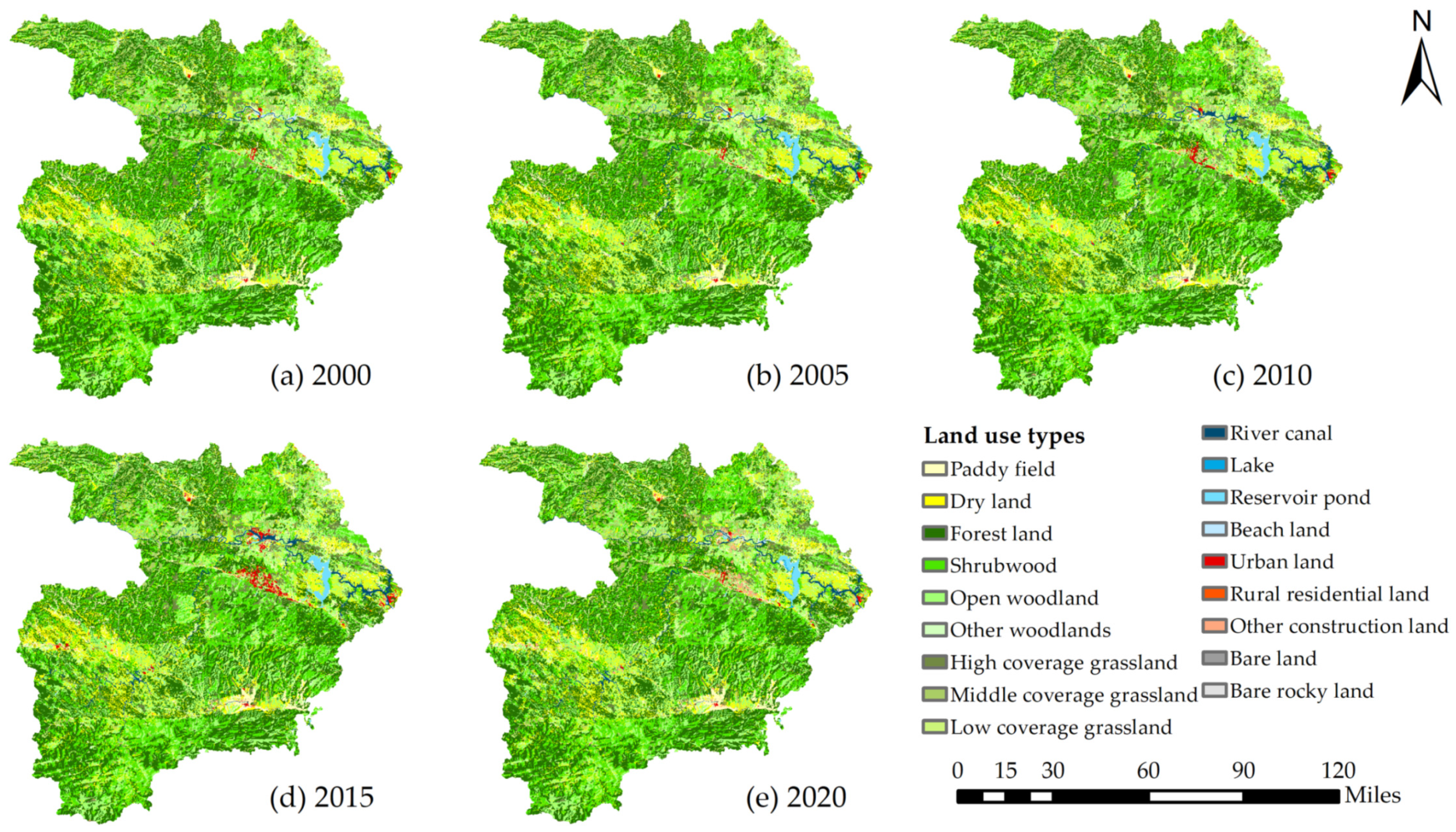
Land 10 00857 g001
Figure 2. Land use types of Shiyan from 2000 to 2020: (a) 2000, (b) 2005, (c) 2010, (d) 2015, and (e) 2020.
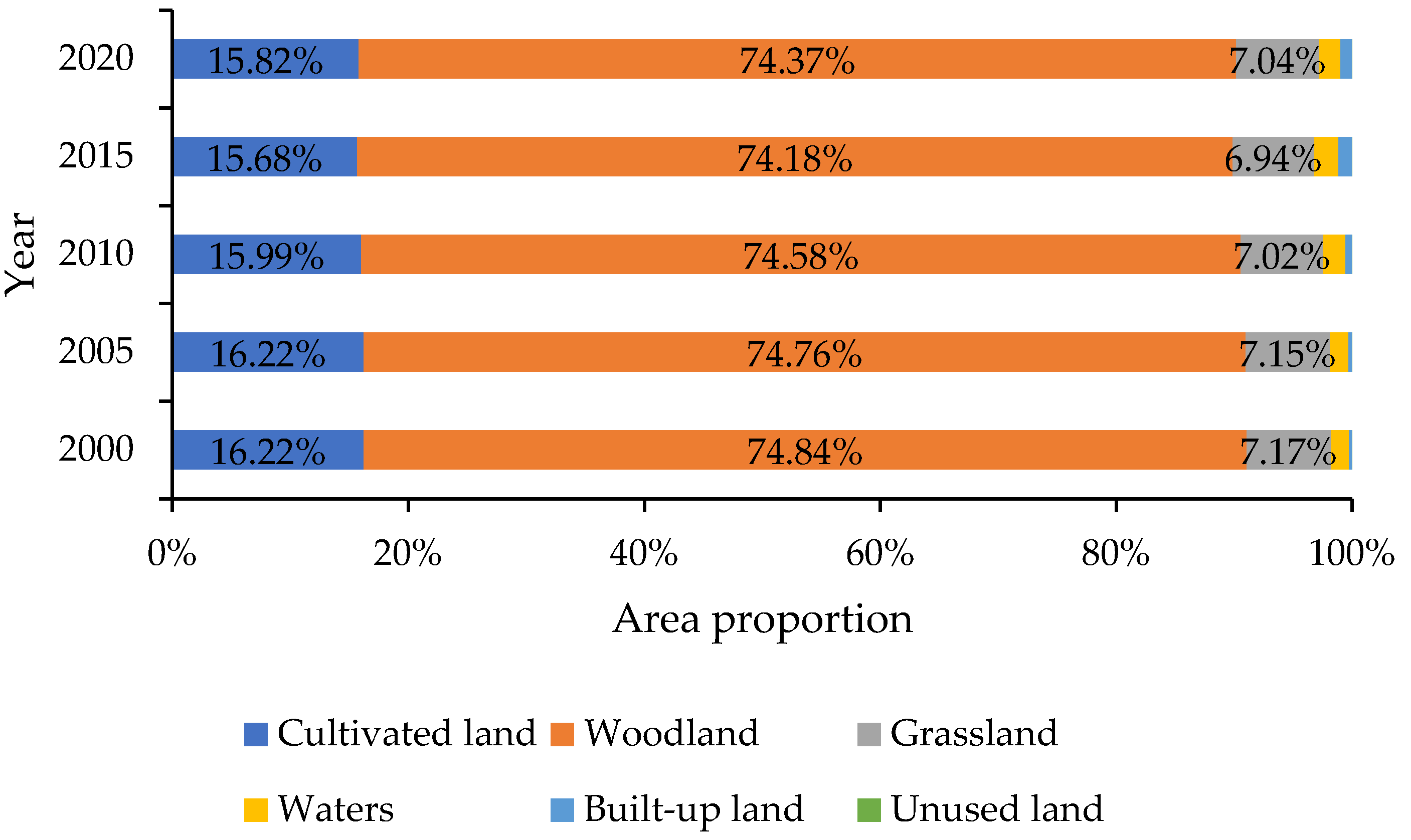
Land 10 00857 g002
Figure 3. Area percentage of land use types in Shiyan from 2000 to 2020.
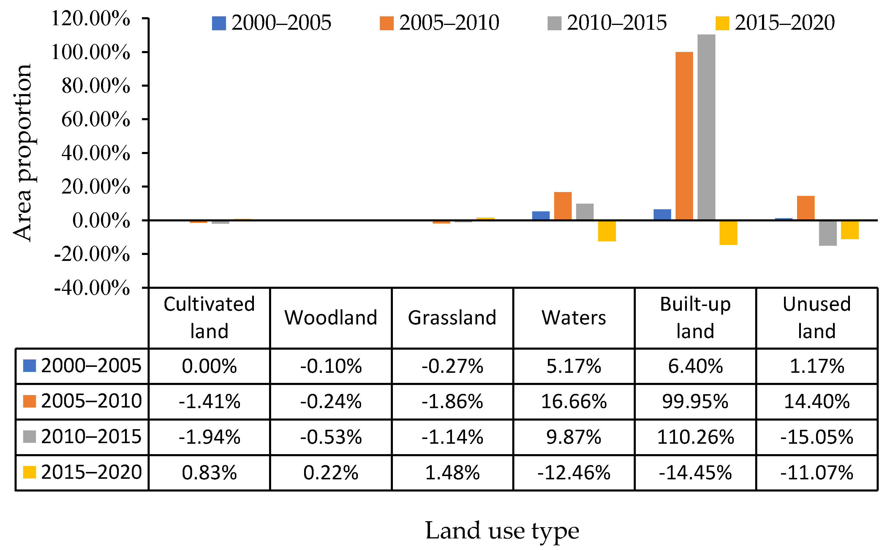
Land 10 00857 g003
Figure 4. Area change percentage of land use types in Shiyan in different periods.
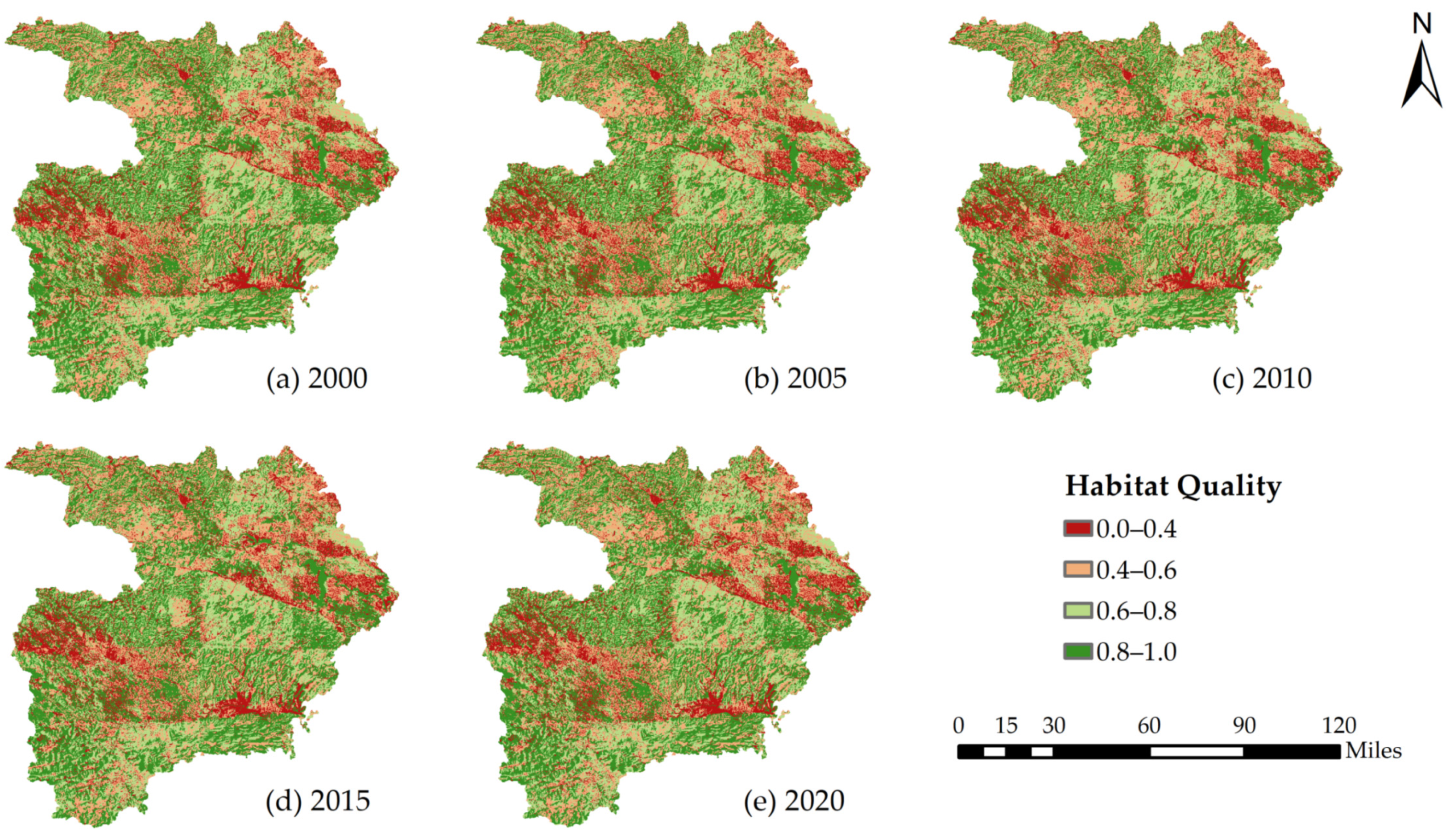
Land 10 00857 g004
Figure 5. Spatial distribution of habitat quality in Shiyan from 2000 to 2020: (a) 2000, (b) 2005, (c) 2010, (d) 2015, and (e) 2020.
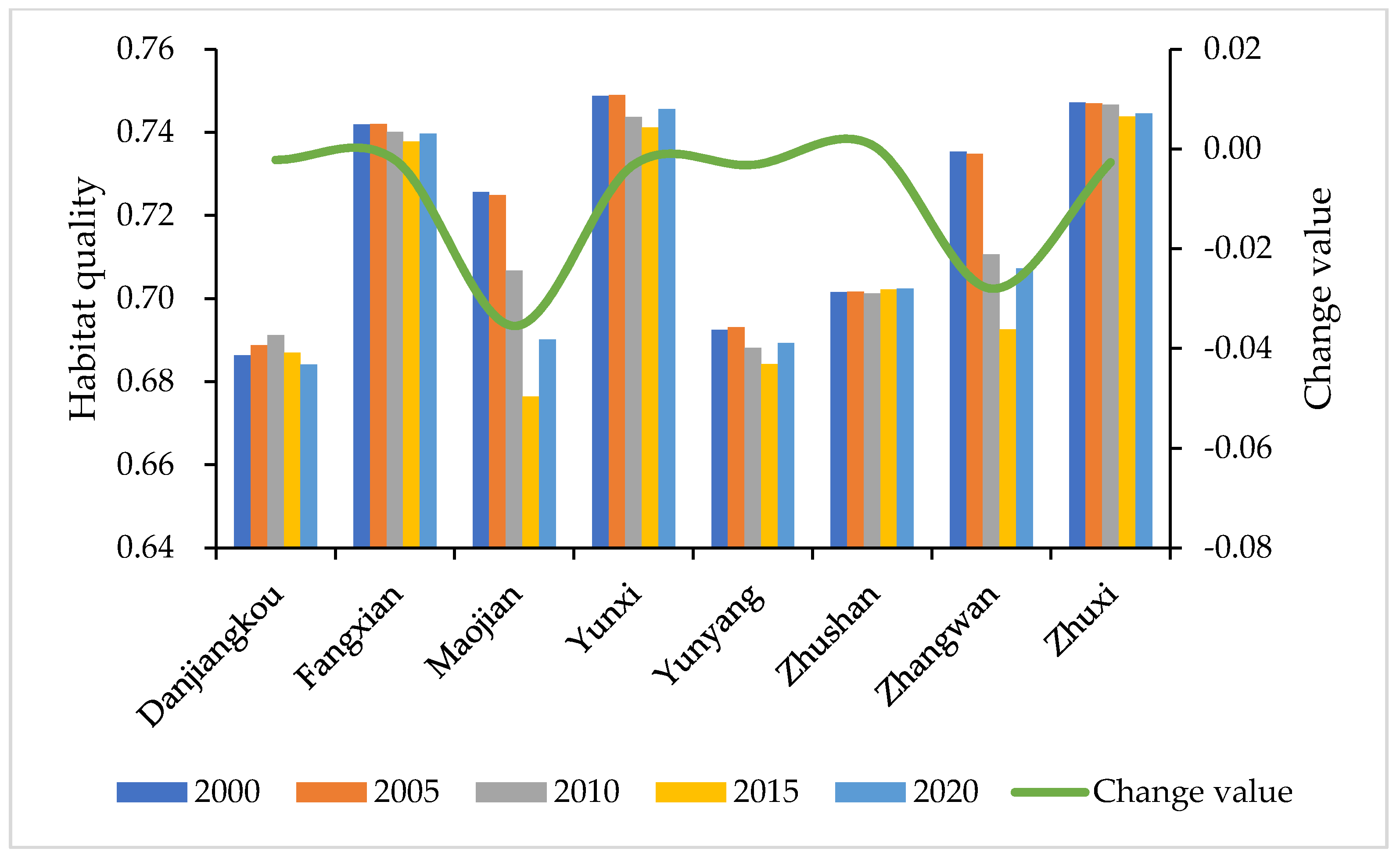
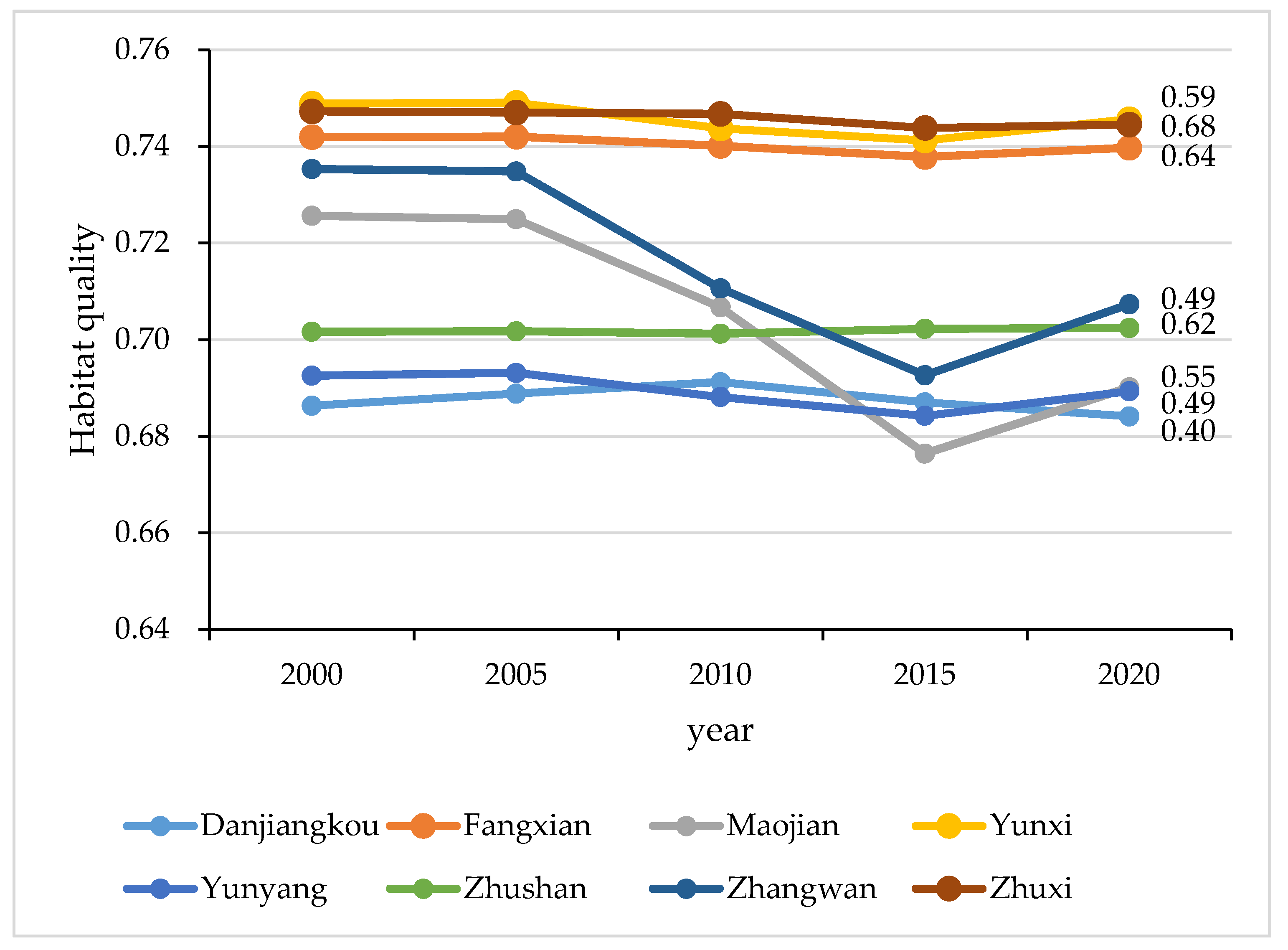
Land 10 00857 g005
Figure 6. Habitat quality change in counties of Shiyan from 2000 to 2020.
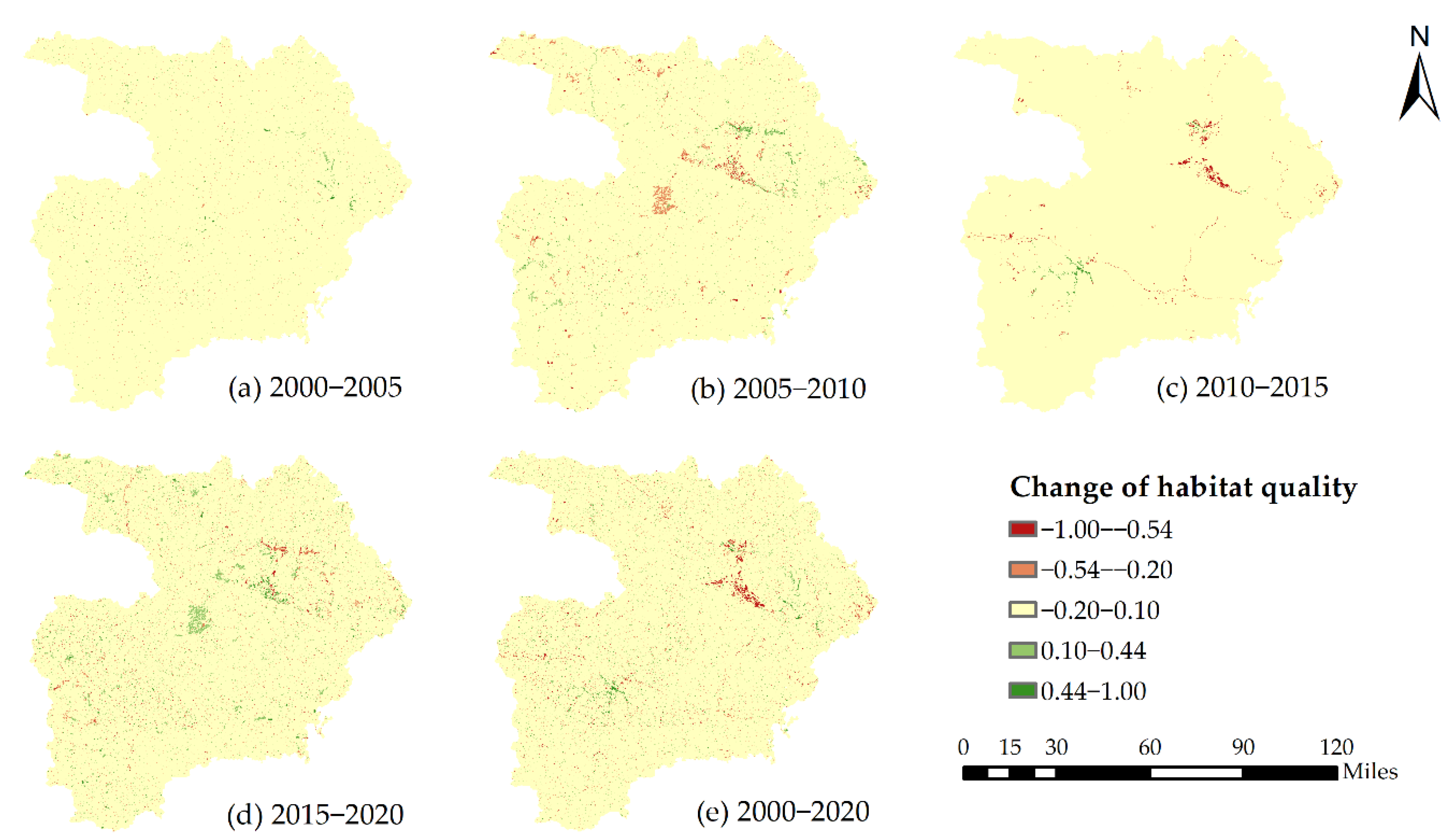
Land 10 00857 g006
Figure 7. Spatial change of habitat quality in Shiyan from 2000 to 2020: (a) 2000–2005, (b) 2005–2010, (c) 2010–2015, (d) 2015–2020, and (e) 2000–2020.
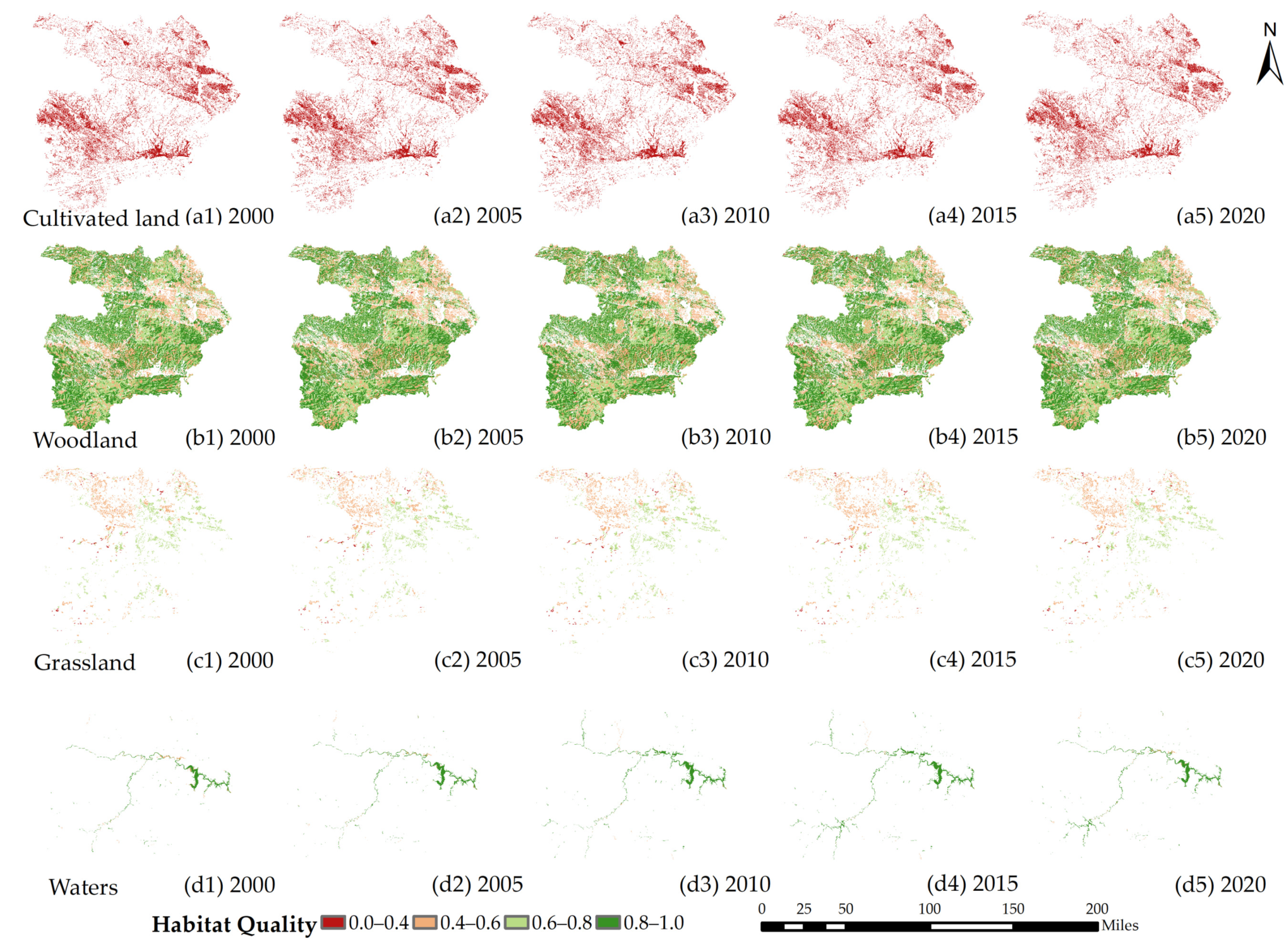
Land 10 00857 g007
Figure 8. Habitat quality change of different land use types in Shiyan from 2000 to 2020. Cultivated land: (a1) 2000, (a2) 2005, (a3) 2010, (a4) 2015, and (a5) 2020; woodland: (b1) 2000, (b2) 2005, (b3) 2010, (b4) 2015, and (b5) 2020; grassland: (c1) 2000, (c2) 2005, (c3) 2010, (c4) 2015, and (c5) 2020; waters: (d1) 2000, (d2) 2005, (d3) 2010, (d4) 2015, and (d5) 2020.
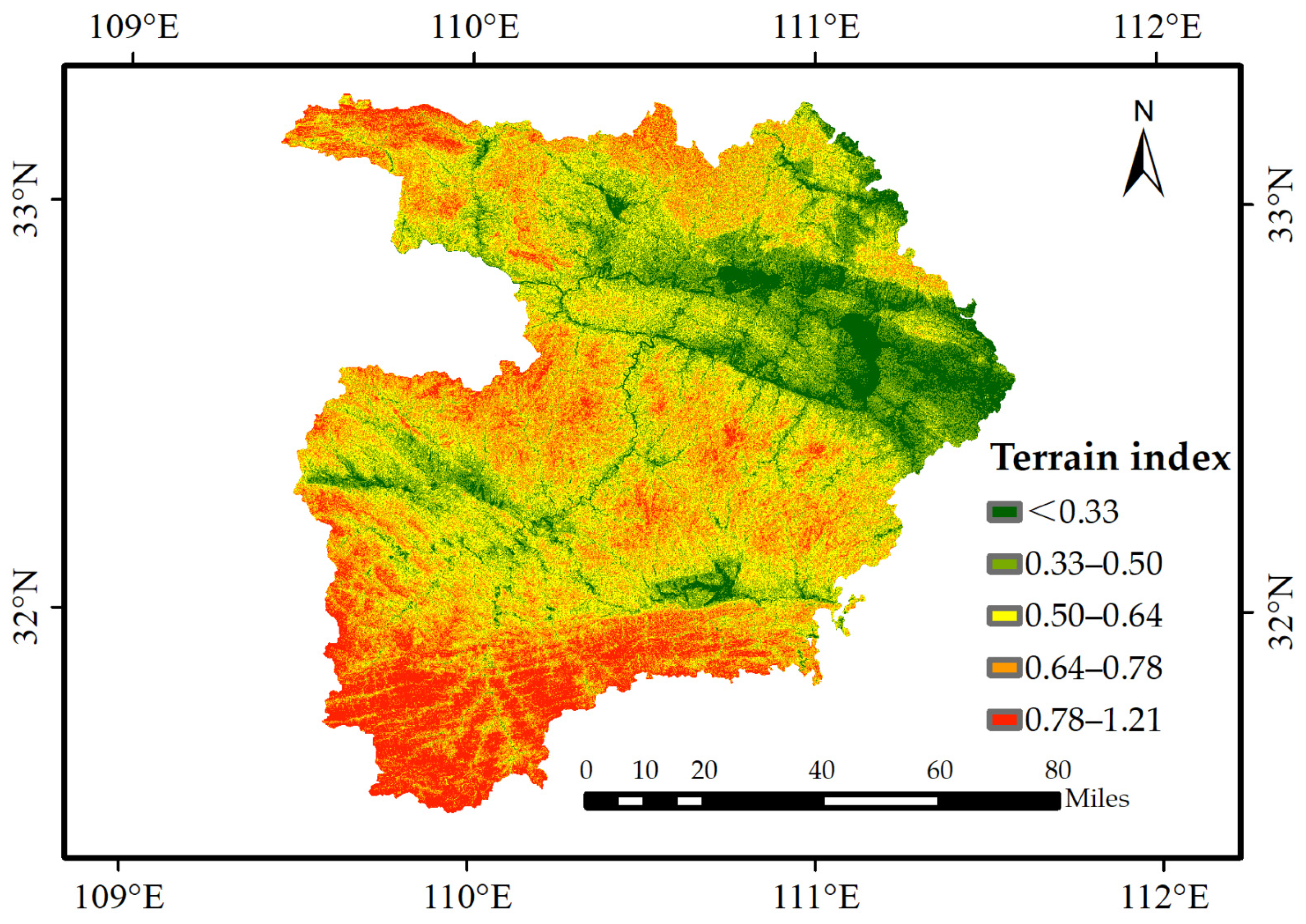
Land 10 00857 g008
Figure 9. Spatial distribution of terrain index values in Shiyan.
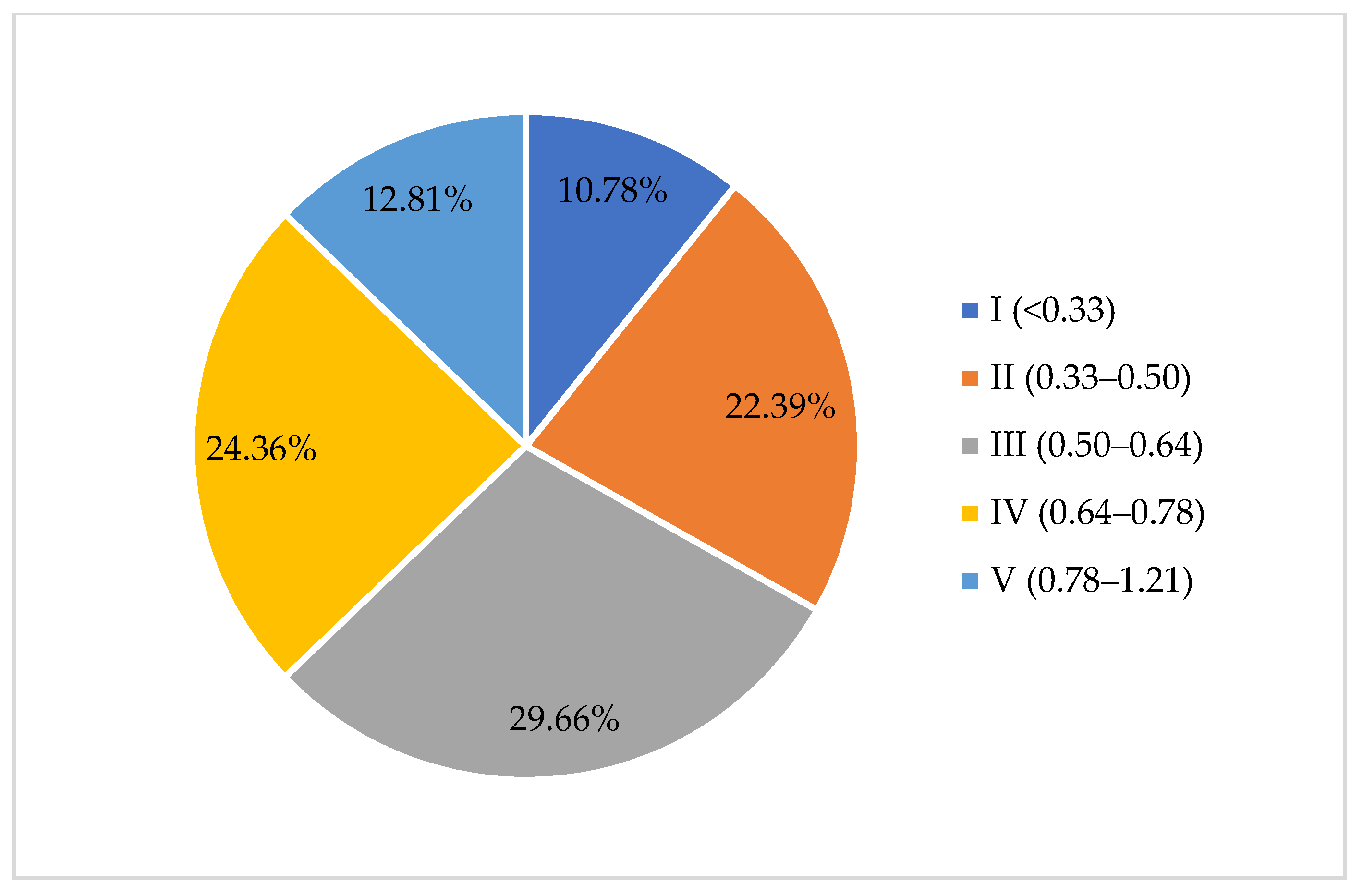
Land 10 00857 g009
Figure 10. Terrain index values classified according to levels and their respective proportions for various locations in Shiyan.
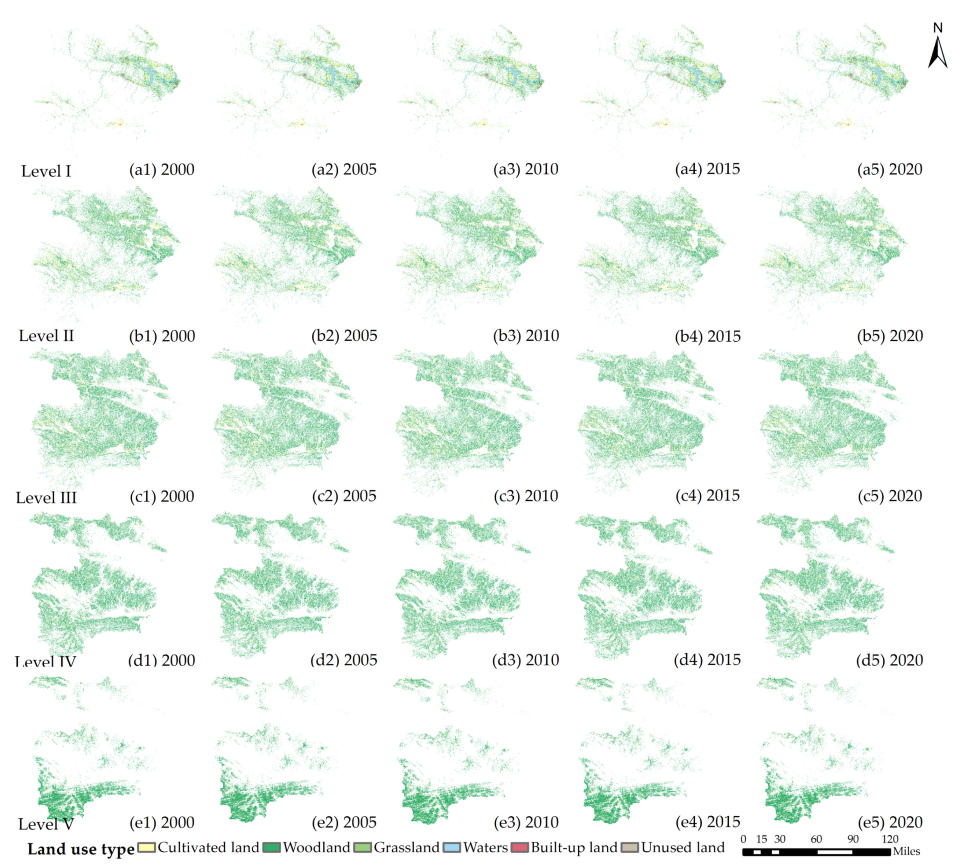
Land 10 00857 g010
Figure 11. Land use change shown for each terrain index level in Shiyan from 2000 to 2020. Level I: (a1) 2000, (a2) 2005, (a3) 2010, (a4) 2015, and (a5) 2020; level II: (b1) 2000, (b2) 2005, (b3) 2010, (b4) 2015, and (b5) 2020; level III: (c1) 2000, (c2) 2005, (c3) 2010, (c4) 2015, and (c5) 2020; level IV: (d1) 2000, (d2) 2005, (d3) 2010, (d4) 2015, and (d5) 2020; level V: (e1) 2000, (e2) 2005, (e3) 2010, (e4) 2015, and (e5) 2020.
Land 10 00857 g011
Figure 12. Relationship between terrain index and habitat quality in the counties of Shiyan from 2000 to 2020. (Note: the values in the column on the right side of the figure correspond to the topographic position index of each county.)
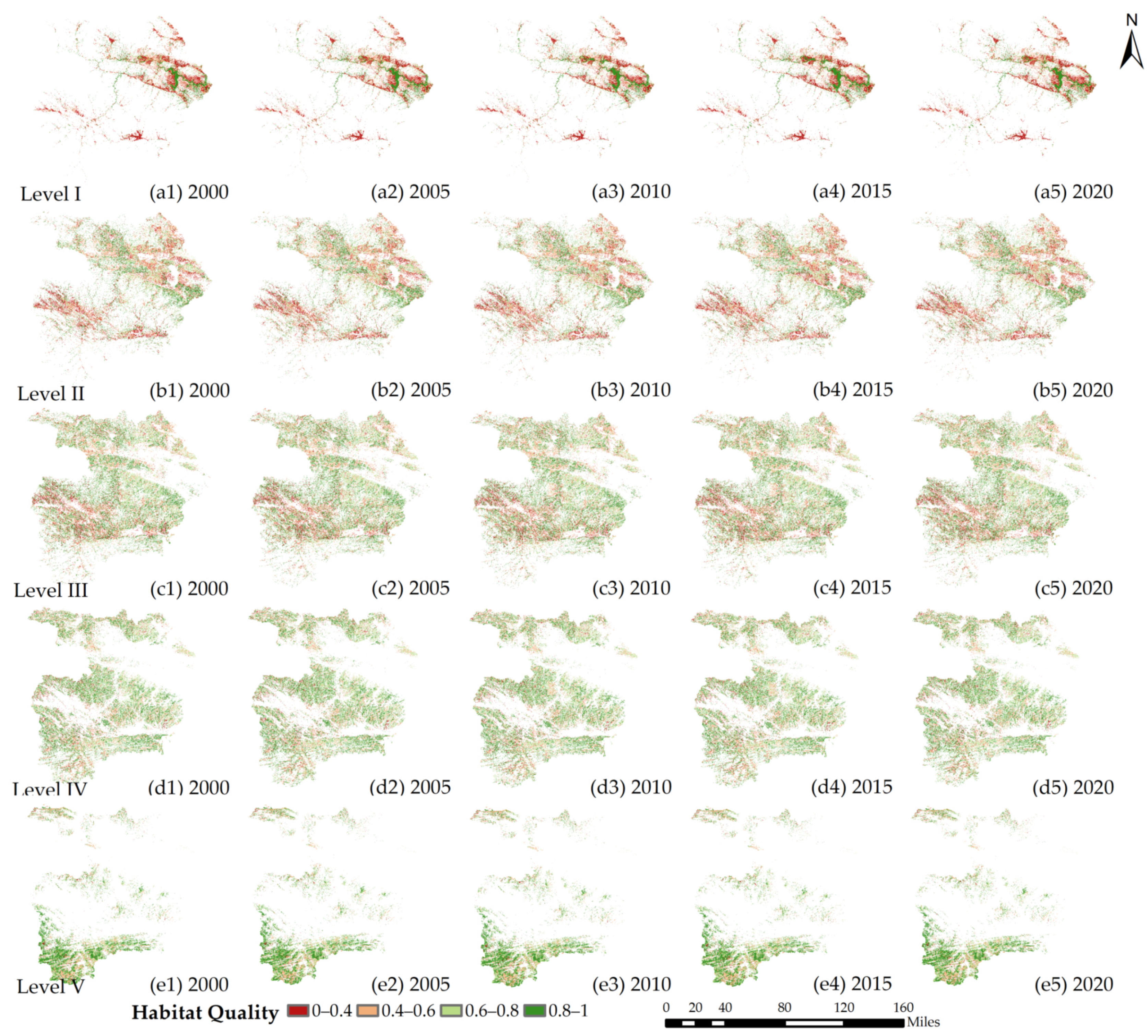
Land 10 00857 g012
Figure 13. Distribution map showing habitat quality for each terrain index level in Shiyan from 2000 to 2020. Level I: (a1) 2000, (a2) 2005, (a3) 2010, (a4) 2015, and (a5) 2020; level II: (b1) 2000, (b2) 2005, (b3) 2010, (b4) 2015, and (b5) 2020; level III: (c1) 2000, (c2) 2005, (c3) 2010, (c4) 2015, and (c5) 2020; level IV: (d1) 2000, (d2) 2005, (d3) 2010, (d4) 2015, and (d5) 2020; level V: (e1) 2000, (e2) 2005, (e3) 2010, (e4) 2015, and (e5) 2020.
Land 10 00857 g013
Table 1. Land use classification and its specific description.
Land Use TypesDescription
First ClassSecond Class
Cultivated landPaddy fieldArable land that has water source guarantees and irrigation facilities that can be irrigated normally in general years for the cultivation of aquatic crops such as rice and lotus root, including the cultivated land where rice and dry land crops are rotated [20].
Dry landArable land without irrigation sources or facilities and which generally does not need seasonal irrigation but relies on natural precipitation for crop growth; dry-grown arable land with water source and irrigation conditions that can be irrigated normally in general years; arable land that is mainly used for vegetable cultivation; fallow land.
WoodlandForest landNatural forest and plantation with >30% canopy density. It includes timber forest, economic forest, shelter forest, and other woodlands.
ShrubwoodLow forest land and shrub forest land with >40% canopy density of <2 m height.
Open woodlandForest land with 10–30% canopy density.
Other woodlandsUncultivated forest land, slash land, nursery, and all types of garden land (orchard, mulberry garden, tea garden, hot forest garden, etc.).
GrasslandHigh coverage grasslandRefers to natural grassland, improved grassland, and mowing grassland covering more than 50%. This type of grassland has better general water conditions with dense grass growth.
Middle coverage grasslandNatural grassland and improved grassland whose coverage is more than 20–50%. This type of grassland is generally lacking in water and has sparse grass cover.
Low coverage grasslandRefers to natural grassland with 5–20% coverage. There is a shortage of grass moisture, grass is sparse, and the conditions for animal husbandry use are poor [21].
WatersRiver canalNatural or artificially excavated rivers and the land is below the annual water level of the trunk. Artificial canals include embankments.
LakeThe land under the perennial water level in naturally formed ponding areas.
Reservoir pondThe land under the perennial water level in artificially built water storage areas.
Beach landThe land between the water level of rivers or lakes during the normal period and the water level of the flood period [22].
Built-up landUrban landThe construction areas of large cities, medium-sized cities, small cities, and counties and towns [23].
Rural residential landThe residential land below the town and independent of the town [24].
Other construction landThe land used for factories and mines, large-scale industrial areas, oil fields, saltworks, quarries, etc., as well as the land for traffic roads, airports, wharves, and special uses that are independent of residential areas at all levels [24].
Unused landBare landSurface soil coverage, vegetation coverage corresponding to less than 5% of the land.
Bare rocky landLand whose surface is rock or gravel, covering more than 5% of the area.
Table 2. Threats and their maximum distance of influence and weight.
ThreatsMaximum Impact Distance (km)WeightDecay
Paddy field10.3exponential
Dry land10.3exponential
Urban land 101exponential
Rural residential land50.6exponential
Other construction land31exponential
Unused land30.1exponential
Main railways40.4linear
Main roads30.4linear
Table 3. Habitat suitability degree and relative sensitivity of habitat types to each threat.
Land Use TypesHabitat SuitabilityThreats
First ClassSecond ClassPaddy FieldDry LandUrban LandRural Residential LandOther Construction LandUnused LandMain RailwaysMain Roads
Cultivated landPaddy field0.40010.500.350.2010.100.20
Dry land0.30100.500.350.2010.100.20
WoodlandForest land10.500.600.900.700.5010.600.80
Shrubwood0.700.300.400.600.400.2010.600.70
Open woodland0.600.500.600.800.600.4010.500.60
Other woodlands0.400.500.600.800.600.4010.400.50
GrasslandHigh coverage grassland0.700.400.450.600.450.3010.100.15
Middle coverage grassland0.600.450.500.650.500.3510.150.20
Low coverage grassland0.400.500.550.700.550.4010.200.25
WatersRiver canal10.500.600.800.600.4010.400.45
Lake0.900.550.650.850.650.4510.450.50
Reservoir pond0.900.600.700.900.700.5010.500.55
Beach land0.600.650.750.950.750.5510.550.60
Built-up LandUrban land000000000
Rural residential land000000000
Other construction land000000000
Unused landBare land000000000
Bare rocky land000000000
Table 4. Habitat quality change in Shiyan from 2000 to 2020.
Habitat Quality LevelValue Range20002005201020152020Change from 2000 to 2020 (%)
Percentage (%)Habitat QualityPercentage (%)Habitat QualityPercentage (%)Habitat QualityPercentage (%)Habitat QualityPercentage (%)Habitat Quality
I0.0–0.416.650.721716.640.722116.640.719216.720.715716.670.71810.02
II0.4–0.622.6822.5422.7522.4422.23−0.45
III0.6–0.824.7824.7524.7724.7424.76−0.02
IV0.8–1.035.8936.0635.8436.0936.330.44
Table 5. Habitat quality change of different land use types in Shiyan from 2000 to 2020.
Land Use TypeYearIIIIIIIVAverage Value of Habitat Quality
Cultivated Land200099.98%0.02%0.00%0.00%0.3326
2005100.00%0.00%0.00%0.00%0.3324
201099.99%0.01%0.00%0.00%0.3315
201599.99%0.01%0.00%0.00%0.3312
202099.98%0.02%0.00%0.00%0.3320
Woodland20000.00%25.28%28.50%46.22%0.8129
20050.00%25.27%28.49%46.25%0.8130
20100.00%25.74%28.64%45.62%0.8097
20150.00%25.42%28.75%45.83%0.8090
20200.00%24.91%28.64%46.45%0.8122
Grassland20000.00%50.32%49.68%0.00%0.6392
20050.00%50.25%49.75%0.00%0.6393
20100.00%50.15%49.85%0.00%0.6392
20150.00%50.45%49.55%0.00%0.6389
20200.00%50.57%49.43%0.00%0.6389
Waters20000.00%0.00%0.00%100.00%0.8978
20050.00%0.00%0.00%100.00%0.9208
20100.00%0.00%0.00%100.00%0.9407
20150.00%0.00%0.00%100.00%0.9463
20200.00%0.00%0.00%100.00%0.9271
Note: Since built-up land is not a habitat and unused land has low habitat quality, they are not considered here.
Table 6. Changes in area percentage represented by land use types for each terrain index level in Shiyan from 2000 to 2020.
Terrain Index LevelYearArea Percentage of Land Use Types/%
Cultivated LandWoodlandGrasslandWatersBuilt-Up LandUnused Land
I (<0.33)20003.75%4.78%0.73%1.26%0.20%0.00%
20053.69%4.78%0.72%1.31%0.21%0.00%
20103.49%4.65%0.69%1.50%0.38%0.00%
20153.33%4.49%0.65%1.57%0.68%0.00%
20203.47%4.61%0.68%1.38%0.55%0.00%
II (0.33–0.50)20005.28%14.30%2.06%0.17%0.05%0.00%
20055.29%14.28%2.05%0.19%0.05%0.00%
20105.27%14.21%2.02%0.23%0.13%0.00%
20155.17%14.04%1.99%0.30%0.36%0.00%
20205.16%14.10%2.01%0.26%0.33%0.00%
III (0.50–0.64) 20004.47%22.65%2.16%0.07%0.01%0.00%
20054.49%22.63%2.16%0.08%0.01%0.00%
20104.50%22.61%2.12%0.10%0.02%0.00%
20154.47%22.55%2.12%0.15%0.08%0.00%
20204.45%22.58%2.14%0.13%0.08%0.00%
IV (0.64–0.78) 20002.17%21.56%1.47%0.01%0.00%0.00%
20052.18%21.54%1.47%0.01%0.00%0.00%
20102.16%21.57%1.44%0.02%0.01%0.00%
20152.16%21.56%1.44%0.03%0.02%0.00%
20202.17%21.55%1.46%0.02%0.02%0.00%
V (0.78–1.21) 20000.56%11.54%0.75%0.00%0.00%0.00%
20050.56%11.54%0.75%0.00%0.00%0.00%
20100.56%11.55%0.74%0.00%0.01%0.00%
20150.56%11.54%0.74%0.00%0.01%0.00%
20200.56%11.53%0.74%0.00%0.00%0.00%
Table 7. Habitat quality for each terrain index level in Shiyan from 2000 to 2020 shown as values.
Terrain Index LevelHabitat QualityChange Value from 2000 to 2020
20002005201020152020
I0.60780.61230.61300.60040.5980−0.0098
II0.66810.66830.66400.65760.6607−0.0074
III0.72890.72880.72530.72360.7269−0.0020
IV0.76940.76920.76620.76530.7683−0.0011
V0.79770.79750.79570.79540.7970−0.0007
Publisher’s Note: MDPI stays neutral with regard to jurisdictional claims in published maps and institutional affiliations.

