
Exploring Effective Built Environment Factors for Evaluating Pedestrian Volume in High-Density Areas: A New Finding for the Central Business District in Melbourne, Australia


Abstract
:1. Introduction
- (1)
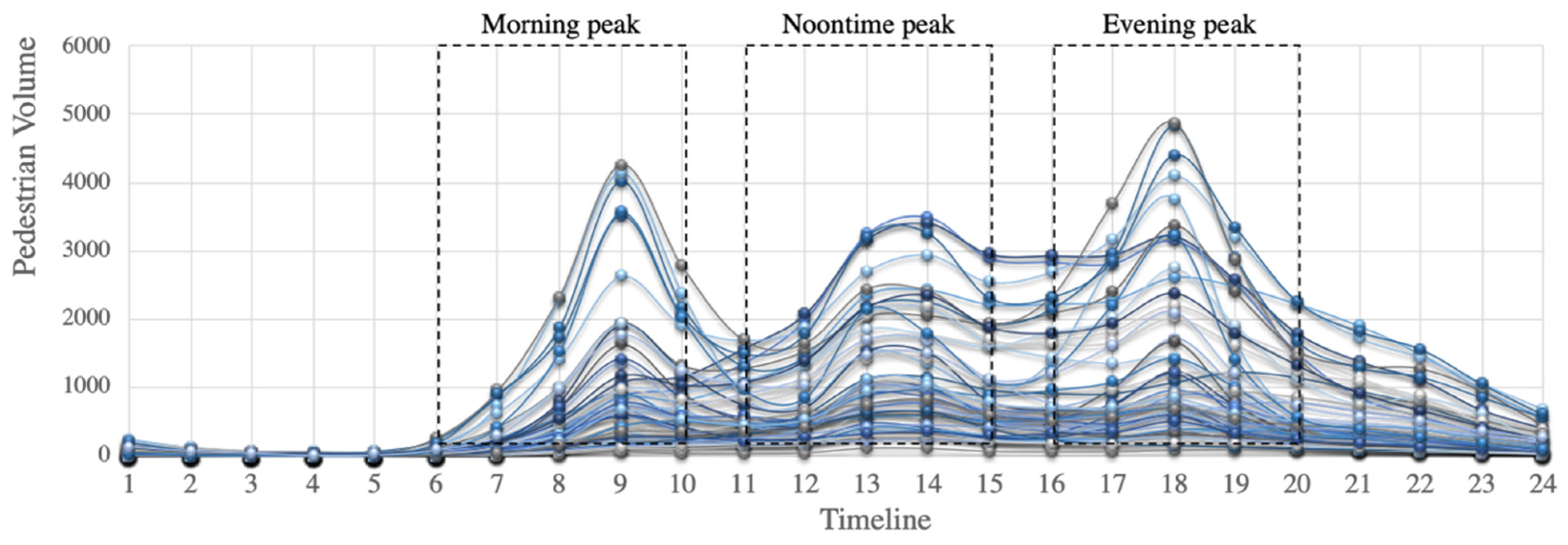
- What are the trends of the pedestrian volume in the Melbourne CBD? (If walking occurred in several peak periods, one would expect to categorize and collect the data during the correlation analysis).
- (2)
- Do all built environment factors under consideration correlate with respect to pedestrian volume during the peak period in a regular grid structured neighbourhood? If not, then can we isolate the irrelevant factor/factors and identify the correlation between built environment factors and pedestrian volume?
- (3)
- What components comprise the principal component analysis, and do these relate to pedestrian volume within the Melbourne CBD?
2. Literature Review
3. Methods and Data
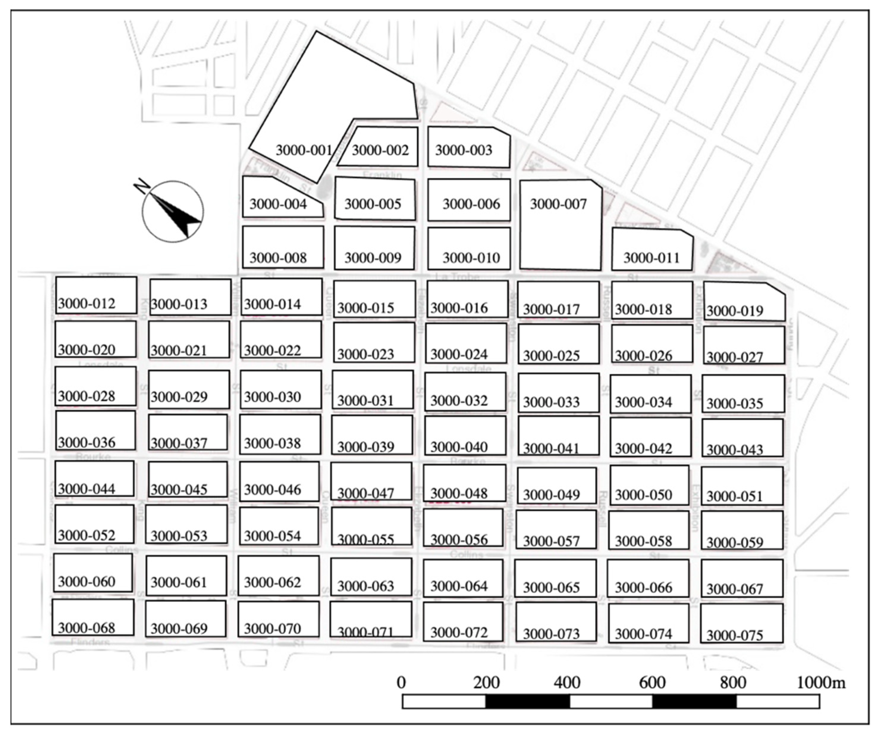
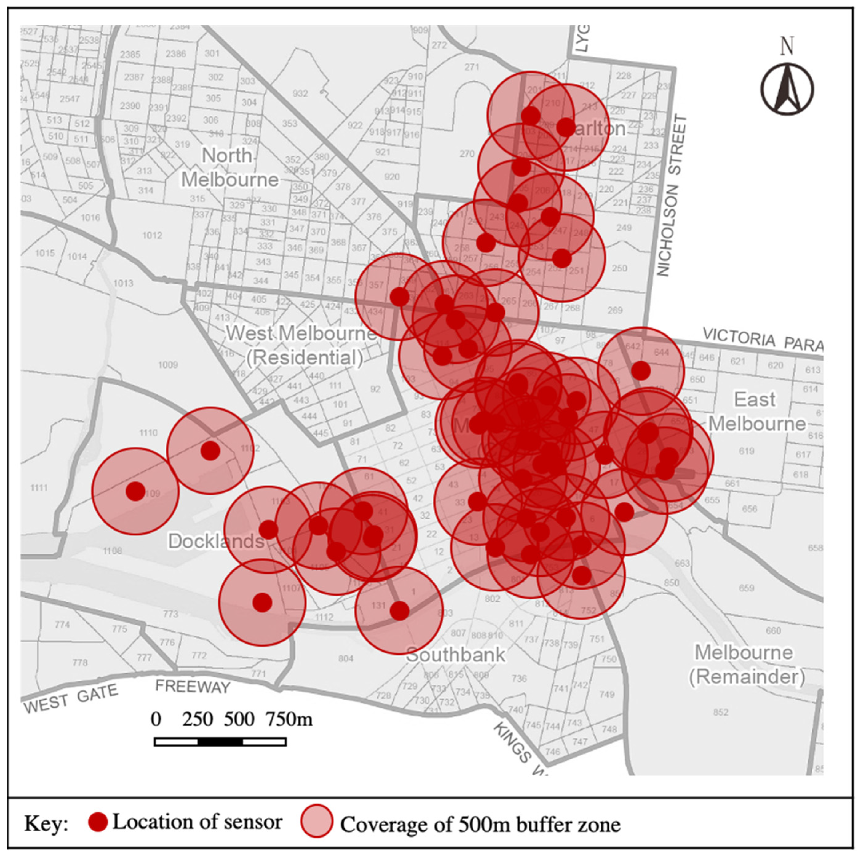
3.1. Study Area
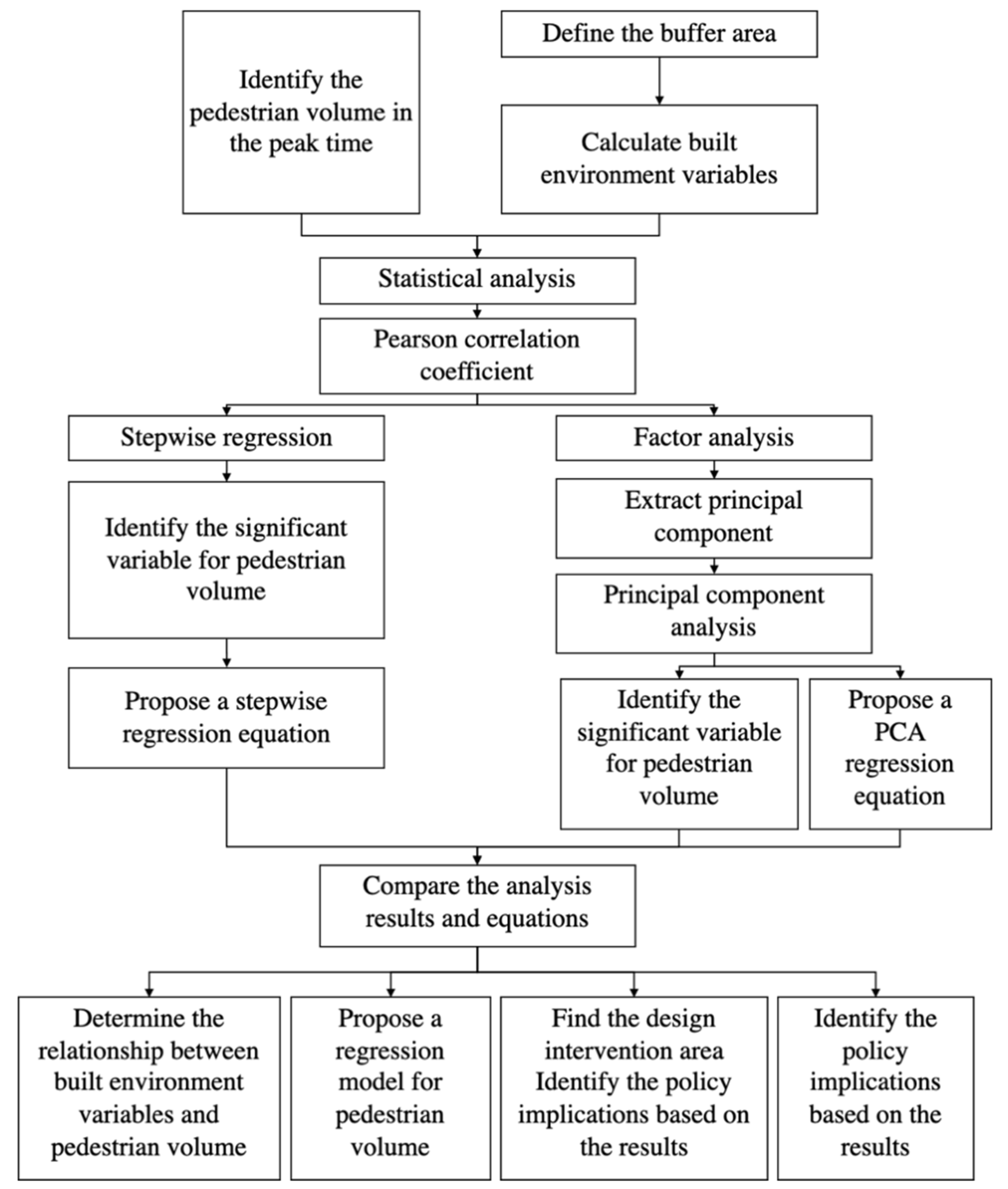
3.2. Study Design
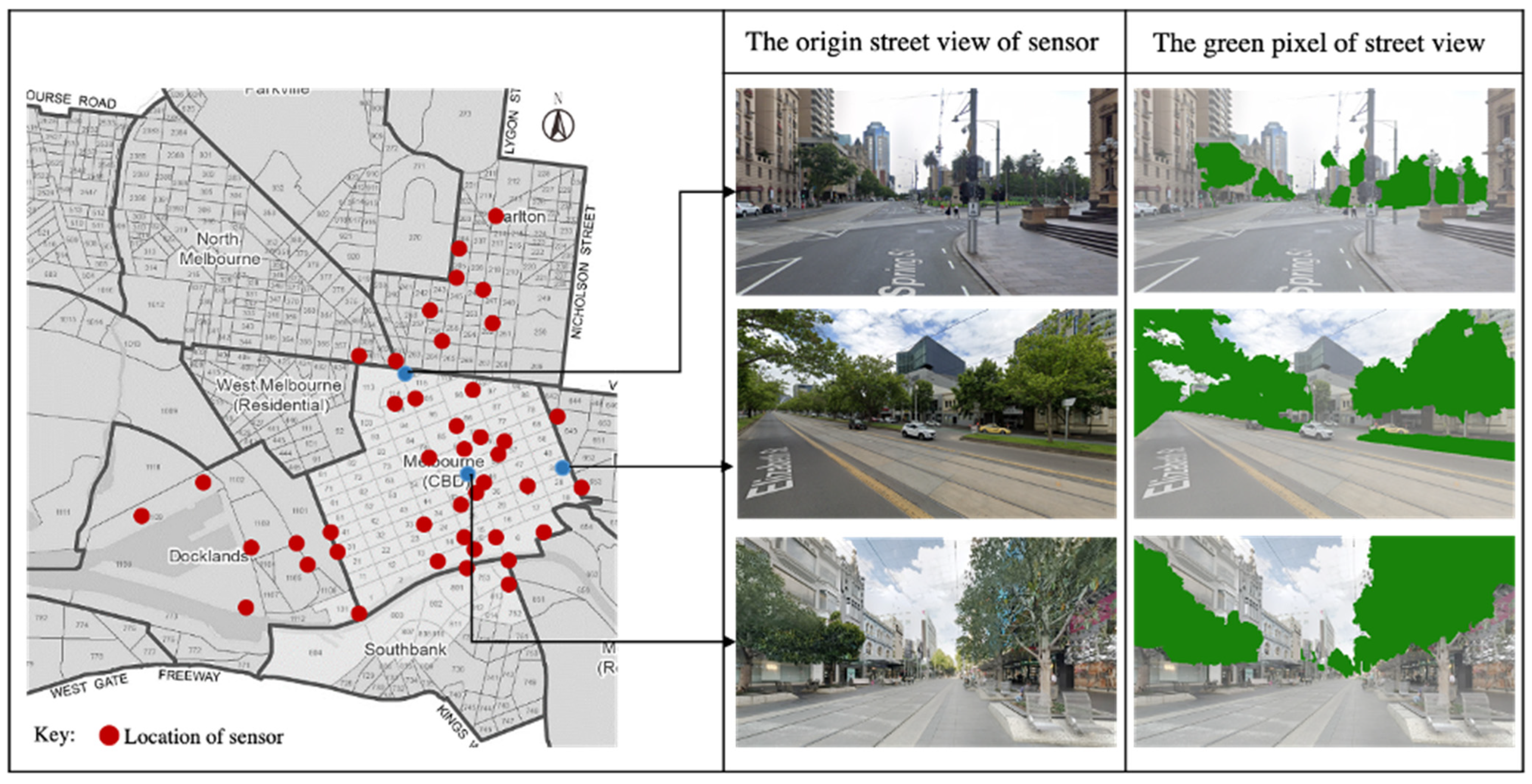
3.3. Data Collection
4. Results
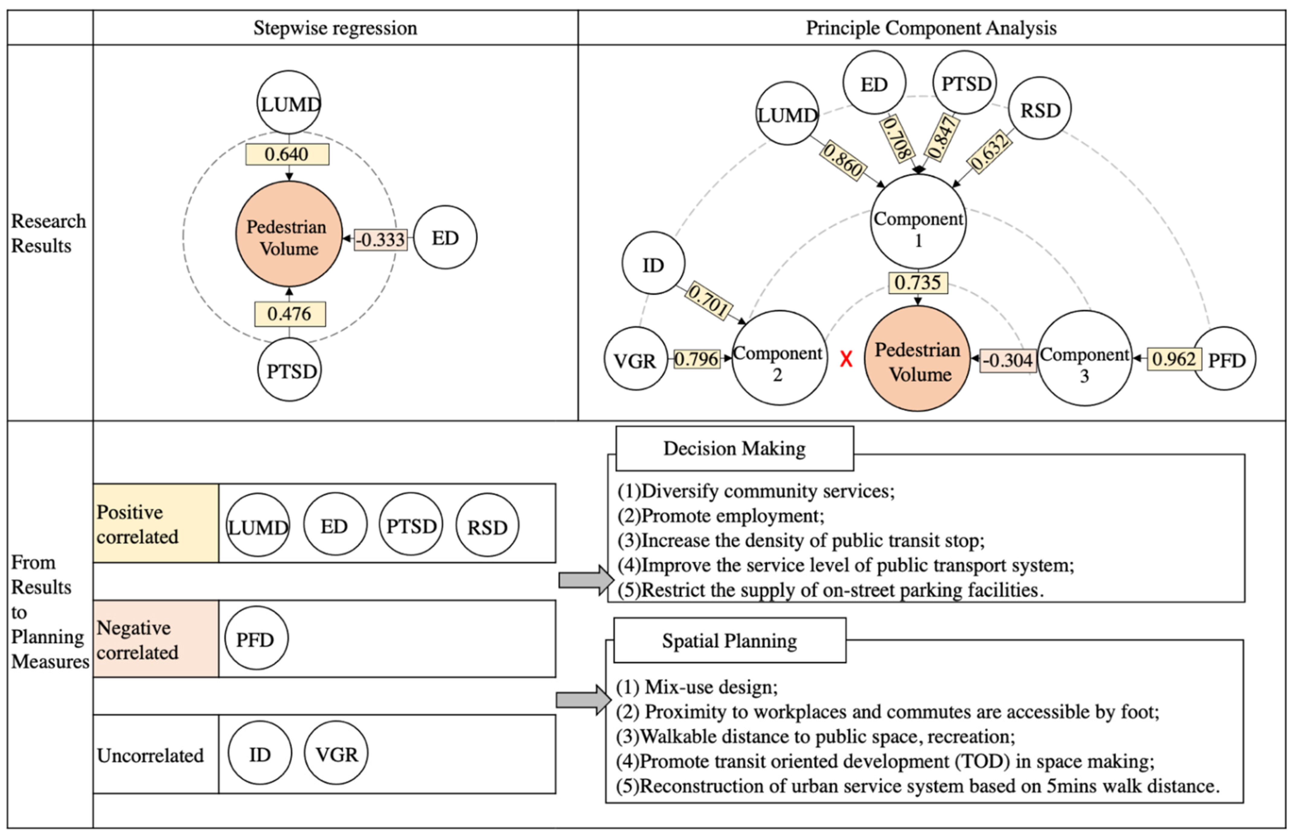
4.1. Summary of Correlation and Stepwise Regression
4.2. Result of Factor Analysis
4.3. Result of Principal Component Analysis
5. Discussion and Design Intervention
6. Conclusions
Author Contributions
Funding
Institutional Review Board Statement
Informed Consent Statement
Data Availability Statement
Conflicts of Interest
References
- Ewing, R.; Cervero, R. Travel and the Built Environment. J. Am. Plan. Assoc. 2010, 76, 265–294. [Google Scholar] [CrossRef]
- Xu, C.; Hu, X.; Tivendale, L.; Liu, C.; Hosseini, M. Building Information Modelling In Sustainable Design And Construction. Int. J. Sustain. Real Estate Constr. Econ. 2018, 1, 164. [Google Scholar]
- Cerin, E.; Nathan, A.; van Cauwenberg, J.; Barnett, D.; Barnett, A. The Neighbourhood Physical Environment and Active Travel in Older Adults: A Systematic Review and Meta-Analysis. Int. J. Behav. Nutr. Phys. Act. 2017, 14. [Google Scholar] [CrossRef] [Green Version]
- Greenwald, M.; Boarnet, M. Built Environment As Determinant of Walking Behavior: Analyzing Nonwork Pedestrian Travel in Portland, Oregon. Transp. Res. Rec. 2001, 1780, 33–41. [Google Scholar] [CrossRef] [Green Version]
- Ewing, R.; Tian, G.; Goates, J.; Zhang, M.; Greenwald, M.; Joyce, A.; Kircher, J.; Greene, W. Varying Influences of the Built Environment on Household Travel in 15 Diverse Regions of the United States. Urban Stud. 2014, 52, 2330–2348. [Google Scholar] [CrossRef]
- Hatamzadeh, Y.; Habibian, M.; Khodaii, A. Measuring Walking Behaviour in Commuting to Work: Investigating the Role of Subjective, Environmental and Socioeconomic Factors in a Structural Model. Int. J. Urban Sci. 2019, 24, 173–188. [Google Scholar] [CrossRef]
- Krizek, K. Operationalizing Neighborhood Accessibility for Land Use-Travel Behavior Research and Regional Modeling. J. Plan. Educ. Res. 2003, 22, 270–287. [Google Scholar] [CrossRef]
- Cervero, R.; Kockelman, K. Travel Demand and the 3Ds: Density, Diversity, and Design. Transp. Res. Part D 1997, 2, 199–219. [Google Scholar] [CrossRef]
- Kerr, J.; Frank, L.; Sallis, J.; Chapman, J. Urban form Correlates of Pedestrian Travel in Youth: Differences by Gender, Race-Ethnicity and Household Attributes. Transp. Res. Part D 2007, 12, 177–182. [Google Scholar] [CrossRef]
- Azmi, D.; Ahmad, P. A GIS Approach: Determinant of Neighbourhood Environment Indices in Influencing Walkability between Two Precincts in Putrajaya. Procedia Soc. Behav. Sci. 2015, 170, 557–566. [Google Scholar] [CrossRef] [Green Version]
- Laatikainen, T.; Haybatollahi, M.; Kyttä, M. Environmental, Individual and Personal Goal Influences on Older Adults’ Walking in the Helsinki Metropolitan Area. Int. J. Environ. Res. Public Health 2018, 16, 58. [Google Scholar] [CrossRef] [Green Version]
- Ewing, R. Pedestrian and Transit-Friendly Design: A Primer for Smart Growth, 1st ed.; American Planning Association: Tallahassee, FL, USA, 1999. [Google Scholar]
- Knuiman, M.; Christian, H.; Divitini, M.; Foster, S.; Bull, F.; Badland, H.; Giles-Corti, B. A Longitudinal Analysis of the Influence of the Neighborhood Built Environment on Walking for Transportation: The RESIDE Study. Am. J. Epidemiol. 2014, 180, 453–461. [Google Scholar] [CrossRef] [PubMed] [Green Version]
- Koohsari, M.; Sugiyama, T.; Mavoa, S.; Villanueva, K.; Badland, H.; Giles-Corti, B.; Owen, N. Street Network Measures and Adults’ Walking for Transport: Application of Space Syntax. Health Place 2016, 38, 89–95. [Google Scholar] [CrossRef] [PubMed]
- Yang, Y.; He, D.; Gou, Z.; Wang, R.; Liu, Y.; Lu, Y. Association Between Street Greenery and Walking Behavior in Older Adults in Hong Kong. Sustain. Cities Soc. 2019, 51, 101747. [Google Scholar] [CrossRef]
- Rollo, J.; Barker, S. Perceptions of Place—Evaluating Experiential Qualities of Streetscapes. In Proceedings of the State of Australian Cities Conference SOAC, Sydney, Australia, 26–29 November 2013. [Google Scholar]
- Ferrer, S.; Ruiz, T.; Mars, L. A Qualitative Study on the Role of the Built Environment for Short Walking Trips. Transp. Res. Part F 2015, 33, 141–160. [Google Scholar] [CrossRef]
- Yin, L.; Cheng, Q.; Wang, Z.; Shao, Z. ‘Big data’ for pedestrian volume: Exploring the use of Google Street View images for pedestrian counts. Appl. Geogr. 2015, 63, 337–345. [Google Scholar] [CrossRef]
- Hajrasouliha, A.; Yin, L. The impact of street network connectivity on pedestrian volume. Urban Stud. 2015, 52, 2483–2497. [Google Scholar] [CrossRef]
- Lee, G.; Jeong, Y.; Kim, S. The Effect of the Built Environment on Pedestrian Volume in Microscopic Space-Focusing on the Comparison between OLS (Ordinary Least Square) and Poisson Regression. J. Asian Archit. Build. Eng. 2015, 14, 395–402. [Google Scholar] [CrossRef] [Green Version]
- Lee, S.; Yoo, C.; Seo, K.W. Determinant Factors of Pedestrian Volume in Different Land-Use Zones: Combining Space Syntax Metrics with GIS-Based Built-Environment Measures. Sustainability 2020, 12, 8647. [Google Scholar] [CrossRef]
- Jiao, J.; Rollo, J.; Fu, B. The Hidden Characteristics of Land-Use Mix Indices: An Overview and Validity Analysis Based on the Land Use in Melbourne, Australia. Sustainability 2021, 13, 1898. [Google Scholar] [CrossRef]
- Population Forecasts—City of Melbourne. Available online: https://www.melbourne.vic.gov.au/about-melbourne/research-and-statistics/city-population/Pages/population-forecasts.aspx (accessed on 6 May 2021).
- Bivina, G.; Gupta, A.; Parida, M. Walk Accessibility to Metro Stations: An Analysis Based on Meso- or Micro-Scale Built Environment Factors. Sustain. Cities Soc. 2020, 55, 102047. [Google Scholar] [CrossRef]
- Gori, S.; Nigro, M.; Petrelli, M. Walkability Indicators for Pedestrian-Friendly Design. Transp. Res. Rec. 2014, 2464, 38–45. [Google Scholar] [CrossRef]
- Hatamzadeh, Y.; Habibian, M.; Khodaii, A. Walking and Jobs: A Comparative Analysis to Explore Factors Influencing Flexible and Fixed Schedule Workers, a Case Study of Rasht, Iran. Sustain. Cities Soc. 2017, 31, 74–82. [Google Scholar] [CrossRef]
- Pedestrian Counting System—City of Melbourne. Available online: https://www.melbourne.vic.gov.au/about-melbourne/research-and-statistics/city-population/Pages/pedestrian-counting-system.aspx (accessed on 5 May 2021).
- Smith, G. Step Away From Stepwise. J. Big Data 2018, 5, 1–12. [Google Scholar] [CrossRef]
- Jolliffe, I.; Cadima, J. Principal Component Analysis: A Review and Recent Developments. Philos. Trans. R. Soc. A 2016, 374, 20150202. [Google Scholar] [CrossRef]
- Nagendra, H. Opposite Trends in Response for the Shannon and Simpson Indices of Landscape Diversity. Appl. Geogr. 2002, 22, 175–186. [Google Scholar] [CrossRef]
- Miserendino, M.; Casaux, R.; Archangelsky, M.; Di Prinzio, C.; Brand, C.; Kutschker, A. Assessing Land-Use Effects on Water Quality, In-Stream Habitat, Riparian Ecosystems and Biodiversity in Patagonian Northwest Streams. Sci. Total Environ. 2011, 409, 612–624. [Google Scholar] [CrossRef] [PubMed]
- Chapman, J.; Marcogliese, D.; Suski, C.; Cooke, S. Variation in Parasite Communities and Health Indices of Juvenile Lepomis Gibbosus across a Gradient of Watershed Land-Use and Habitat Quality. Ecol. Indic. 2015, 57, 564–572. [Google Scholar] [CrossRef]
- Jiao, J.; Fu, B. Overview and Applicability of Land Use-mixed Indices in the Smart City. In Proceedings of the 2020 4th International Conference on Smart Grid and Smart Cities (ICSGSC), Osaka, Japan, 18–21 August 2020. [Google Scholar]
- CLUE. Available online: https://data.melbourne.vic.gov.au/stories/s/CLUE/rt3z-vy3t?src=hdr (accessed on 5 May 2021).
- Walk Score Methodology. Available online: https://www.walkscore.com/methodology.shtml (accessed on 5 May 2021).
- Li, X.; Zhang, C.; Li, W.; Ricard, R.; Meng, Q.; Zhang, W. Assessing Street-Level Urban Greenery Using Google Street View and a Modified Green View Index. Urban For. Urban Green. 2015, 14, 675–685. [Google Scholar] [CrossRef]
- Kaiser, H. An Index of Factorial Simplicity. Psychometrika 1974, 39, 31–36. [Google Scholar] [CrossRef]


| . | Adjust Coefficients | |
|---|---|---|
| Intersection density coefficient () | Intersection per buffer zone | |
| Over 20 | 1.000 | |
| 15 to 20 | 0.990 | |
| 12 to 15 | 0.980 | |
| 9 to 12 | 0.970 | |
| 6 to 9 | 0.960 | |
| Under 6 | 0.950 | |
| Distance decay coefficient () | Distance to the sensor (meter) | |
| Less than 300 | 1.000 | |
| 300 to 500 | 0.975 | |
| 500 to 1000 | 0.750 | |
| Service level coefficient () | Transportation means | |
| Heavy/light rail | 2.000 | |
| Ferry/cable car/tram | 1.500 | |
| Bus | 1.000 |
| Obs. | Mean. | S.D. | Min | Max | ||
|---|---|---|---|---|---|---|
| Built environment variables | Land-use mix degree | 52 | 1.558 | 0.269 | 0.958 | 2.186 |
| Employment density | 52 | 35.121 | 23.779 | 1.700 | 95.492 | |
| Parking facility density | 52 | 8.613 | 4.399 | 1.398 | 20.152 | |
| Intersection density | 52 | 0.034 | 0.011 | 0.010 | 0.054 | |
| Public transit stop density | 52 | 0.141 | 0.048 | 0.038 | 0.214 | |
| Visible green ratio | 52 | 0.200 | 0.112 | 0.002 | 0.450 | |
| Restaurant seating density | 52 | 17.847 | 11.061 | 1.950 | 53.640 | |
| Pedestrian volume | Morning | 52 | 594.465 | 668.648 | 13.000 | 3973.000 |
| Noontime | 52 | 1070.119 | 849.471 | 51.000 | 3628.000 | |
| Evening | 52 | 1124.539 | 1014.242 | 68.000 | 4631.000 |
| Pedestrian Volume | |||
|---|---|---|---|
| Morning Peak (6:00 to 10:00) | Noon Peak (11:00 to 15:00) | Evening Peak (16:00 to 20:00) | |
| Land−use mix degree | 0.510 ** | 0.723 ** | 0.659 ** |
| Employment density | 0.285 * | 0.279 * | 0.239 |
| Parking facility density | −0.128 | −0.304 * | −0.263 |
| Intersection density | −0.153 | 0.099 | 0.021 |
| Public transit stop density | 0.388 ** | 0.627 ** | 0.556 ** |
| Visible green ratio | −0.168 | −0.066 | −0.130 |
| Restaurant seating density | −0.061 | 0.335 * | 0.261 |
| Unstandardized Coefficients | Standardized Coefficients | t | p | VIF | R2 | Adjust. R2 | ||
|---|---|---|---|---|---|---|---|---|
| B | Std. Error | Beta | ||||||
| Constant | −2710.893 | 417.483 | −6.493 | 0.000 ** | 0.668 | 0.647 | ||
| Land−use mix diversity | 1930.980 | 313.004 | 0.640 | 6.169 | 0.000 ** | 1.555 | ||
| Public transit stop density | 8114.663 | 1854.990 | 0.476 | 4.375 | 0.000 ** | 1.667 | ||
| Employment density | −11.379 | 3.671 | −0.333 | −3.099 | 0.003 ** | 1.710 | ||
| Initial Eigenvalues | Rotation Sums of Squared Loadings | |||||
|---|---|---|---|---|---|---|
| Total | Variance Explained Rate (%) | Cumulative (%) | Total | Variance Explained Rate (%) | Cumulative (%) | |
| Component 1 | 2.911 | 41.737 | 41.737 | 2.441 | 34.871 | 34.871 |
| Component 2 | 1.269 | 18.122 | 59.858 | 1.500 | 21.428 | 56.299 |
| Component 3 | 1.129 | 16.136 | 75.994 | 1.379 | 19.695 | 75.994 |
| Component 4 | 0.801 | 11.442 | 87.436 | |||
| Component 5 | 0.387 | 5.528 | 92.964 | |||
| Component 6 | 0.302 | 4.313 | 97.278 | |||
| Component 7 | 0.191 | 2.722 | 100.000 | |||
| Component 1 | Component 2 | Component 3 | |
|---|---|---|---|
| Diversity of Land Use and Amenities | Walking Friendly | Vehicle Parking Friendly | |
| Land−use mix degree | 0.860 | −0.160 | −0.055 |
| Employment density | 0.708 | 0.231 | 0.504 |
| Parking facility density | −0.041 | −0.098 | 0.962 |
| Intersection density | 0.275 | 0.701 | −0.107 |
| Public transit stop density | 0.847 | 0.254 | −0.095 |
| Visible green ratio | −0.077 | 0.796 | 0.043 |
| Restaurant seating density | 0.632 | 0.471 | 0.416 |
| Component 1 | Component 2 | Component 3 | |
|---|---|---|---|
| Diversity of Land Use and Amenities | Walking Friendly | Vehicle Parking Friendly | |
| Land−use mix degree | 0.459 | −0.289 | −0.145 |
| Employment density | 0.235 | 0.017 | 0.292 |
| Parking facility density | −0.119 | −0.092 | 0.745 |
| Intersection density | 0.003 | 0.481 | −0.135 |
| Public transit stop density | 0.373 | 0.022 | −0.185 |
| Visible green ratio | −0.207 | 0.621 | 0.021 |
| Restaurant seating density | 0.160 | 0.217 | 0.228 |
| Unstandardized Coefficients | Standardized Coefficients | t | p | VIF | R2 | Adjust R2 | ||
|---|---|---|---|---|---|---|---|---|
| B | Std. Error | Beta | ||||||
| Constant | 0.019 | 0.001 | 14.988 | 0.00 ** | − | 0.641 | 0.618 | |
| Component 1 (diversity of land use and amenities) | 0.011 | 0.001 | 0.735 | 8.494 | 0.001 ** | 1.000 | ||
| Component 2 (walking friendly) | −0.001 | 0.001 | −0.089 | −1.030 | 0.308 | 1.000 | ||
| Component 3 (vehicle parking friendly) | −0.005 | 0.001 | −0.304 | −3.515 | 0.001 ** | 1.000 | ||
Publisher’s Note: MDPI stays neutral with regard to jurisdictional claims in published maps and institutional affiliations. |
© 2021 by the authors. Licensee MDPI, Basel, Switzerland. This article is an open access article distributed under the terms and conditions of the Creative Commons Attribution (CC BY) license (https://creativecommons.org/licenses/by/4.0/).
Share and Cite
Jiao, J.; Rollo, J.; Fu, B.; Liu, C. Exploring Effective Built Environment Factors for Evaluating Pedestrian Volume in High-Density Areas: A New Finding for the Central Business District in Melbourne, Australia. Land 2021, 10, 655. https://doi.org/10.3390/land10060655
Jiao J, Rollo J, Fu B, Liu C. Exploring Effective Built Environment Factors for Evaluating Pedestrian Volume in High-Density Areas: A New Finding for the Central Business District in Melbourne, Australia. Land. 2021; 10(6):655. https://doi.org/10.3390/land10060655
Chicago/Turabian StyleJiao, Jiacheng, John Rollo, Baibai Fu, and Chunlu Liu. 2021. "Exploring Effective Built Environment Factors for Evaluating Pedestrian Volume in High-Density Areas: A New Finding for the Central Business District in Melbourne, Australia" Land 10, no. 6: 655. https://doi.org/10.3390/land10060655