Article

A Geospatial Approach to Measure Social Benefits in Urban Land Use Optimization Problem

by
Md. Mostafizur Rahman
1,2,* and
György Szabó
1
1
Department of Photogrammetry and Geoinformatics, Faculty of Civil Engineering, Budapest University of Technology and Economics, 3 Műegyetem rkp., K Building First Floor 31., H-1111 Budapest, Hungary
2
Department of Urban and Regional Planning, Rajshahi University of Engineering and Technology, Rajshahi 6204, Bangladesh
*
Author to whom correspondence should be addressed.
Land 2021, 10(12), 1398; https://doi.org/10.3390/land10121398
Submission received: 20 November 2021 / Revised: 14 December 2021 / Accepted: 15 December 2021 / Published: 17 December 2021
(This article belongs to the Special Issue Land: 10th Anniversary)

Abstract

:
Different conflicting objectives are used in urban land use optimization problems. The maximization of social benefit is one of the important objectives in urban land use optimization problems. Many researchers have used different methods to measure social benefits in land use optimization. Studies show that there is no established method to measure social benefit in the urban land use allocation game. Against this background, this study aims to (a) identify the appropriate indicators as a measure of social benefit, and (b) propose a composite index to measure social benefit in urban land use optimization problems. Based on the literature review and expert opinion, this study identifies four indicators as a measure of social benefit. These are spatial compactness, land use compatibility, land use mix, and evenness of population distribution. Using the weighted sum approach, this study proposes a composite social benefit index (SBI) to measure social benefit in urban land use allocation/optimization problems and planning. The study suggests that spatial compactness is the most influential indicator to the SBI, but the most critical indicator is compatibility, whose 11.60% value reduction from 0.5 alters the decision of choice. Finally, the proposed method was applied in Rajshahi city in Bangladesh. The result suggests the potential of using SBI in the land use allocation problem. It is expected that the proposed social benefit index (SBI) will help the land use optimization and planning and will be helpful for decision makers.

1. Introduction

Land use optimization is a key strategy for achieving long-term balanced urban growth through economic prosperity, resource efficiency, environmental protection, and social equality [1,2,3]. Due to the involvement of multiple stakeholders, there are conflicting interests in urban land use optimization. For example, if residential development occurs in a low-lying area, it may solve the housing problem, but it will lead to the problem of urban drainage. If green space is replaced by urban buildings, due to urbanization, urban environment and health will be negatively impacted. Land developers want to maximize their economic profits while government tries to maximize social benefits from land use allocation. Different conflicting objectives are used in urban land use optimization problems. Some of the objectives are used most frequently in urban land use optimization problems. The most important objectives include maximization of economic benefits, maximization of ecological benefits, maximization of environmental benefits, minimization of land conversion cost, maximization of land value, maximization of land use compatibility, maximization of accessibility, maximization of compactness, maximization of ecosystem service value (ESV), and maximization of social benefits [4].
Maximization of social benefits is one of the important objectives in urban land use optimization problems. Cities face a wide range of social challenges. The city develops as a unique interaction among inhabitants, contacts, social ties, and direct and indirect communication interactions, rather than just buildings, roads, parks, fences, abandoned corners, water lines, and cable networks [5]. Concern regarding social well-being becomes a crucial prerequisite for a sustainable society and city. Social sustainability ensures equality, democracy, and diversity in our cities. In the present scenario of urban land transformation, urban ecosystem disturbance reduces the urban social efficiency of city space, which requires deliberate intervention to increase social interaction and public space [6,7]. For a city to be sustainable, it is mandatory that the city is socially linked through public space, design, and interaction regardless of social, cultural, and economic backgrounds which creates the opportunity for an accessible city. When a city offers a diverse range of opportunities for everyday life, it becomes more alive and appealing, which can improve the people’s quality of life. Furthermore, a socially sustainable city allows people’s health to be supported through urban places built for physical activity and socialization [8].
In response to the growing concern of social well-being toward urban sustainability, many researchers included maximizing social benefits in urban land use optimization problems. However, in our previous study [4], we identified that there is no generalized method to calculate the social benefit in the land use allocation problem. Many researchers tried to maximize social benefits in their land use optimization problems using different methods [9,10]. For example, Zhang et al. [11] measured social benefit as a function of social security service value, Yuan et al. [10] used the spatial compactness of an area as a measure of the social benefit, and Cao et al. [9] considered spatial accessibility as an indicator of social sustainability. However, we argue that only a single indicator may not be the optimal measure of social benefit. Our claim is also supported by some other studies. For example, Jenks and Jones [12] mentioned that although spatial compactness in the city has many social benefits, this compaction may lead to reduced living space, poorer access to green spaces, less affordable housing, and poorer health. Even a compact city may derive negative consequences if there exists incompatibility among land uses. If the land uses are compatible but there is a lack of accessibility, it will also reduce the social benefit. So, compatibility and accessibility are also the aspects of measuring social benefit. Similarly, there may be other indicators contributing to the measure of social benefit. Thus, we believe that multiple indicators can be attributed to the measure of social benefit. So, some kind of composite index is required to measure social benefit. However, in our previous study [4], we identified that there is no such established method to measure social benefit in the land use allocation game. Against this background, this study aims to (a) identify the appropriate indicators as a measure of social benefit, and (b) propose a composite index to measure social benefit in urban land use allocation.
The rest of the paper is structured as follows. Section 2 presents a brief literature review on the indicators used to measure social benefits from land use planning. 
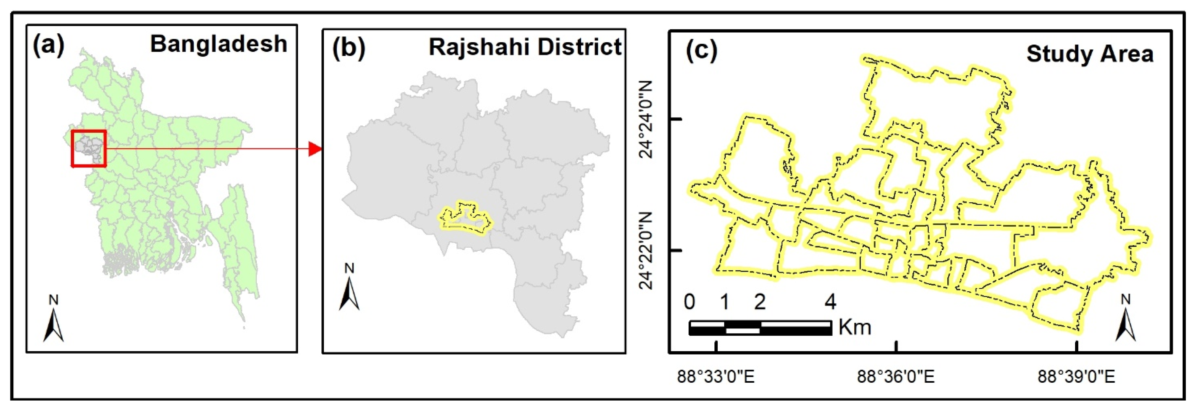
Section 3 describes the data used in this study and the methods followed for constructing the social benefit index (SBI). The result of this study is presented in Section 4. This section illustrates the development of SBI. The section also contains the application of SBI in a real-world city. Finally, this paper ends with Section 5, which contains the limitation, future scope of the work, and concluding remarks.

2. Literature Review

Urban land use planning is becoming a critical issue in the face of rapid urbanization and sustainability challenges. Sustainability has been the main concern in urban land use planning for the past decade. This emphasized the inclusion of environmental, economic, and social dimensions of sustainability in urban land use planning. Although the environmental dimension was the main concern in sustainable development in the early stage, debates within urban sustainability literature have moved beyond solely environmental concern to economic and social dimensions [12]. A significant portion of the sustainable development literature now emphasizes the importance of considering social benefits in urban land use planning [13,14,15,16,17]. For example, Eizenberg and Jabareen [13] identified that social benefit was integrated late in the urban sustainable development debate, and they developed a conceptual framework to incorporate the social benefits into spatial planning. Medved et al. [14] also explored that social benefits have received little attention in the built-environment discipline. In their study, they focused on the connection and interaction between urban planning and social sustainability. Williams [16] worked on urban design and social benefits. He showed that better land use planning could ensure more social benefits to the residents, including a healthy, safe, accessible, friendly, and attractive environment.
To reflect the urban social sustainability, many researchers incorporated social benefits in their land use optimization problems and planning [13,16,17,18,19,20]. This section discusses different types of spatial indicators available in the literature to measure the urban social benefits.
A significant number of studies [2,10,21,22] considered spatial compactness as an indicator of social benefit. A systematic review on land use optimization by Rahman and Szabó [4] showed that maximization of spatial compactness is frequently used as one of the optimization objectives in many urban land use optimization problems. In those studies, spatial compactness is used as an indicator of urban social benefits, thinking that a compact city is more sustainable and livable [23], can maximize the social well-being of the people [24], can provide better accessibility to city facilities; can promote social equity education, health, and living [25]; and can offer a higher level of personal satisfaction, social interaction, and perceived physical health benefits [26]. However, this indicator alone cannot be sufficient for measuring social benefit because other studies show that although spatial compactness in the city has many social benefits, this compaction may lead to reduced living space, poorer access to green spaces, less affordable housing, and poorer health [12]. So, in addition to spatial compactness, other indicators should be considered while measuring social benefits. Different methods were used to measure urban spatial compactness. The most common methods used to measure spatial compactness include (a) non-linear integer program-neighbor method; (b) linear integer program-neighbor method; (c) minimization of shape index; (d) linear IP using aggregated blocks/minimization of the number of clusters per land use types; (e) linear integer program using buffer cells; and (f) spatial autocorrelation [27]. The non-linear integer program is the simplest explanation for land use compactness, which relies solely on the neighbors of each cell to calculate compactness by sum. The linear integer program model is an analogous linear reformulation of the first, with the inclusion of integer variables [28]. The minimization of shape index method calculates each cluster’s form index, which sounds complicated but it is a good way to describe compactness [29]. The fourth concept is to group individual cells into blocks and create a model that reduces the number of blocks in the final allocation result that contains only one land use category. In other words, the goal is to reduce the number of clusters by as much as possible for each land use category. The fifth method is stated as a problem in which parcels are chosen, and each reserve (one land use type) is divided into core cells and a buffer zone. Compactness is achieved indirectly by reducing the number of buffer cells surrounding the core sections [30]. The last option is to use Moran’s I, and other geographical statistics to calculate spatial compactness [31].
The land use compatibility is considered a crucial factor in urban development planning. It refers to the situation in which adjacent land uses can co-exist without creating any negative effects. Land use compatibility has a strong connection with many aspects of social gain in cities. Hence, it is considered to be another criterion of urban social benefit in relation to land use planning. Land use compatibility is used in many urban land use optimization problems and planning, thinking that compatibility among adjacent land uses will derive more social benefits to the urban people [3,32,33,34,35,36]. Land use compatibility has significance in social sustainability and social well-being through increased social interactions, good human–environment interaction, a pleasant and healthier environment, and increasing livability [35]. Although a compact city generates many social benefits, it may degrade the health and livability of people and derive more negative consequence if there exist incompatibility among land uses, for example, industrial activities beside residential land [37]. If there is a lack of compatibility among the adjacent urban land uses, it may lead to incongruous urban land development, and a polluted environment [38]. Effective urban planning and social benefits can be achieved if urban land uses allocation is happened in an ideal situation to avoid negative impacts from adjacent land uses. Adjacent land uses may create negative externalities on other land uses through inter-land use interaction if the spatial structure of land uses is incompatible to each other [39]. So, land use compatibility is an important factor of urban social well-being. Different methods, including the score card method, expert opinion method, analytical hierarchy process (AHP) method, Delphi method, etc., are used to derive the compatibility of land uses. While the main principle of deriving the compatibility values is the judgment of the expert in the respective field, the computation method is somewhat different. However, the most widely used method to derive compatibility value is AHP [40] since this method is straightforward. In this method, land use types are compared on a scale between 1 and 9 based on a group of experts. Based on the pairwise comparison, the final compatibility value is derived.
Land use mix is a widely discussed subject of social sustainability and overall urban sustainability. It refers to the degree of diversity among the different land use types within an area. Land use mix is considered a measure of social benefit since the land use mix provides many benefits to the city. These include short trip generation, easy access to facilities, reduced transport cost and travel length, reduced emission, etc. It is an important component of walkability [41]. The capacity to locate different types of functions (residential, commercial, institutional, and recreational) within walking or cycling distance is a benefit of mixed land use. Land-use policies have shown that mix-use design is a good method to promote non-automobile forms of transportation [42]. At the microlevel, Gehrke and Clifton [43] stated that mixed land use as a strategy has a substantial association with walking. Other studies have also found a link between active commuting, accessibility, and walkability through mixed land use [44]. It is one of the foundations for urban sustainability against functional segregation in land use policies. In many studies, land use mix is considered an integral part of land use allocation problem and planning on the reasoning that mixed land use promotes social well-being of urban population [45,46,47]. Mixed land use is a prerequisite for urban proximity dynamics, healthier lifestyles, and public space vitality [48]. Land use mix has significance in deriving social well-being and benefits from urban land use allocation. Mixed land uses promote walkability, shorten trip length, reduce emission, save energy and resources, ensure effective use of urban infrastructure and services, and increase social interactions [49]. The quantification of land use mix can take numerous forms. One method is to quantify the degree of land use mix and investigate the relationship between built environment characteristics (such as urban density, distance, destination accessibility, and transportation network structure) and individual movement in cities [50]. Different methods, including clustering index (CLST), activity related complementarity index (ARC), balance index (BAL), entropy index (ENT), Herfindahl–Hirschman index (HHI), dissimilarity index (DIS), Gini index (GINI), and mixed degree index (MDI), are used to measure land use mix in a city [51]. However, the CLST, ARC, MDI, and GINI indices were seen in limited use in the literature due to their limitations. The ENT, DIS, and HHI were found to be the most successful methods for quantifying land use mix in most of the research. Previous research has employed the ENT to determine the land use mix status. The term ENT refers to an area that has a mix of different forms of land use. The HHI refers to the land use mixed status and is used to describe a state of market concentration. DIS, according to researchers, is a method of determining the balance status of a specific area’s land use mix [52]. However, due to the computation simplicity and more meaningful applicability, the ENT is discussed and used widely in many research works as a way of presenting the diversity of land use mix. The spatial distribution of population in the city is another criterion to measure social benefits that people gain from the city. Cities provide many functions and opportunities to the urban people. In welfare economics, the functions and benefits that people derive from the city are known as utility [53]. Studies suggest that spatial distribution of population within a city has a strong relationship with health and the social well-being [54]. This requires the population in city to be distributed in such a manner that can maximize the per capita utility from the city. If the population distribution is not optimal or homogeneous, then it will create spatial disparity in social benefits of the city people [55]. For example, if there are two green spaces of similar size and functions in a city but if these green spaces have different coverage area and serve different numbers of population, then the per capita utility values from the green spaces will be different, which may create spatial disparity in terms social benefits and well-being. Similarly, if the population density in a given area is more or less than the ideal population density then the resources (public utilities, open space, health facilities, etc.) will be either burdened or underutilized. So, optimal population distribution is important to maximize the per capita utility or social benefits within the city. Evenness is one of the techniques to measure the homogenous distribution of any geographical phenomena. Evenness expresses how evenly the individuals in the community are distributed over the different species. Different methods are used to measure the evenness in the spatial distribution. These include the Alatalo evenness index, Menhinnick evenness index, Simpson’s dominance index, Shannon–Wiener evenness index, etc. [49]. All these indices use block or zone to represent the evenness of distribution. One problem with these methods is that they cannot be applied in a single cell considering the attribute of the cell concerned. Rather, multiple cells forming zone are used to calculate the value of evenness.
The above literature suggests that several factors are linked with urban social benefits. A single indicator alone cannot reflect the social benefits from land use allocation. Hence, multiple indicators are required to measure the social benefits.

3. Data and Methods

3.1. Study Area

The study was conducted in Rajshahi City, Bangladesh. The city is located on the north bank of the Padma River which runs through the southern side of the city. The city is located near the Bangladesh–India border and lies between 24°20′57.03″ to 24°20′58.40″ North Latitude and 88°32′30.19″ to 88°40′08.76″ East Longitude, with an area of 48.05 km2 (Figure 1). The total population of the city is about 0.76 million. The topography of the city is predominantly flat, having a mean surface elevation of 21.289 m above sea level. Rajshahi is an important administrative, educational, cultural, and business center in Bangladesh. Under the Köppen climate classification, Rajshahi has a tropical wet and dry climate. The climate of Rajshahi is generally marked with monsoons, high temperatures, considerable humidity, and moderate rainfall.
The first formal master plan of the city in connection with the Rajshahi metropolitan area (RMA) was prepared in 2004 with a vision to guide the future land use development of the city. This plan was supposed to update every five years to accommodate required changes and to ensure planned development. However, due to a lack of sufficient manpower, resources, and regulation, the plan was not updated in timely fashion that created unplanned development of the city. Realizing the necessity, recently, the Rajshahi development authority has taken initiative to revise the land use plan to ensure guided development in the city.

3.2. Data

The main goal of this study is to develop a composite index to measure social benefits from urban land use allocation. To achieve the goal, we used two kinds of data: (a) hypothetical data, and (b) real-world data. Hypothetical data were used to develop a social benefit index (SBI), and the proposed SBI was applied to real-world data. Rajshahi city of Bangladesh was selected to apply the proposed SBI. For hypothetical data, we used a raster dataset of 30 × 30 grid as a planning area with six land use types. This land uses area residential, commercial, green space, industrial, educational institution, and health facilities. It may be noted that the hypothetical dataset was also used in many studies including urban land use optimization and allocation problems [56,57,58]. In addition to land use data, we also used hypothetical population data. The land use and population data are presented in Figure 2. For real-world data, we used land use and population data of Rajshahi city, Bangladesh. These data were collected from the Rajshahi Development Authority (RDA) of Bangladesh. Figure 3 represents the land use data of Rajshahi city. All data were processed in ArcGIS 10.8 and MS Excel 2016 software.

3.3. Methods

3.3.1. Selection of Indicators

In order to develop a composite index of social benefit, it is necessary to select the appropriate indicators that reflect social benefits from land use allocation. To select the indicators, first, a literature review was conducted. Based on the literature review, we selected some indicators that can be used to measure social benefit. The literature review was presented earlier in Section 2 of this paper. Then the findings of the literature review were shared with 15 experts, comprising urban planners, architects, and environmental experts. The expectation is that the experts will come to a conclusion regarding the indicators of social benefits. In the next step, a semi-structured interview was done with those experts, and final indicators were selected based on the literature review and expert opinions.

3.3.2. Computation of Indicators

Based on the literature review and expert opinions, we identified four indicators as a measure of social benefits in land use optimization problems. In this section, the computation approach of those indicators is discussed.

3.3.2.1. Spatial Compactness

Spatial compactness is a numerical quantity that represents the degree to which different land use types are compact in nature in terms of spatial distribution. Several measures of spatial compactness exist in the literature. These include (a) linear integer programming (IP)-neighbor method; (b) non-linear IP-neighbor method; (c) linear IP using buffer cells; (d) spatial autocorrelation; and (e) minimization of shape index [9,27,56,57]. Among these methods, the non-linear IP-neighbor method and minimization of shape index are the most popular and straightforward. However, computation of the non-linear IP-neighbor method is based on Moore’s eight-cell neighborhood method [59], and the shape index is based on patches of land parcel [60]. Comparing the suitability and simplicity, this study used Moore’s eight-cell neighborhood method to compute the spatial compactness of urban land allocation. In this method, spatial compactness is represented by the number of cells allocated for the same use in each cell’s eight neighboring cells (Equation (1)) [1].
S p a t i a l   c o m p a c t n e s s = k = 1 K i = 1 N j = 1 M b i j k x i j k  
where,
b i j k = x i 1   j   k + x i + 1   j   k + x i   j 1   k + x i   j + 1   k + x i 1   j 1   k + x i 1   j + 1   k + x i + 1   j 1   k + x i + 1   j + 1   k
In the above Equation (1), K is the number of land use types, and K = 5. N and M are the total numbers of rows and columns of the planning area, respectively, and N = M = 30. When a cell (i, j) is allocated for land use k, x i j k = 1 ; otherwise x i j k = 0 . After calculating the spatial compactness for every cell, we can calculate the total compactness for a land use allocation scenario by adding the compactness of each cell under study.
Initially, the spatial compactness was calculated as the number of same land use types around a cell within an eight-neighborhood region. So, the minimum and maximum value of spatial compactness could be 0 and 8 respectively. However, this value is not comparable with other indicators. So, we normalized the value of spatial compactness using the min-max normalization method (Jain and Bhandare, 2013). Now the value of normalization ranges from 0 to 1. The higher value of spatial compactness means that the land distribution is more compact. On the other hand, a lower value of spatial compactness indicates that the land use distribution is scattered. Due to the many benefits of the compact city, it is desired that the form of the city is compact in nature to derive the social benefits to the city people.

3.3.2.2. Land use Compatibility

Land use compatibility measures the degree to which adjacent land uses are compatible. It is an important consideration in urban land use planning. If the land uses are not compatible with each other, it will create many problems for the city people. There are different land use types in the urban area. Each land use has its preference to be with another category of land use type(s) within its neighborhood. One kind of land use may be compatible with some land use type(s) but may be incompatible with other land use type(s) in its immediate neighborhood. Even if one land use type is compatible with another land use type, the degree of compatibility may be different. Hence, compatibility indices are required to measure the compatibility of a specific land use type with other land use type within its immediate neighborhood. Then we can judge the compatibility of a land use allocation scenario by summing up the compatibility indices for all cells in the study area.
The land use compatibility indices are generated from expert opinion or stakeholder response. Previous studies used the same approach to derive land use compatibility [1,2,61]. In this study, we interviewed 15 experts consisting of urban planners, landscape architects, and environmental experts to obtain compatibility scores among different land use types. The interview was done with the hope that they would come up with the best possible outcome. However, the compatibility score is likely to change from one expert to another. So, first, a pair-wise comparison approach was followed to generate the comparative weight of each pair of land use types [62]. After deriving the comparative weight values, we generated the final compatibility values using the AHP method [40]. The method of AHP is described in Section 3.3.3. The result of the AHP values is represented either as normalized priorities or idealized priorities. Normalized priorities are the direct result of AHP, whereas idealized values are derived by dividing each priority by the largest one. In idealized priorities, the largest value is converted to 1. In our study, we computed compatibility values in an idealized form for better comparison.
According to Moore’s neighborhood (n = 1) concept, for any cell, there are eight neighboring cells [59]. The compatibility value depends on the two adjacent land use types. The total compatibility for each cell depends on the land use type of its neighboring cells. Based on the derived compatibility value, the compatibility for each cell of land use was calculated using Equation (2).
L a n d   u s e   c o m p a t i b i l i t y = i = 1 N j = 1 M C o m p a t i b i l i t y   k i k j
where ki and kj represent the land use types of the vector i and its neighbor j, and the compatibility between them is represented by C o m p a t i b i l i t y   k i k j . In addition,
k = 1 , , k ; i = 1 , , N ; a n d   j = 1 , , M
After calculating the value of each cell, we normalized the value of land use compatibility using the min-max normalization method (Jain and Bhandare, 2013).

3.3.2.3. Land Use Mix

Land use mix is a measure that counts the percentage of two or more land use types in a given area. There are different types of indices to measure the degree of land use mix in a given area. The most important of them includes the balance index (BAL), activity-related complementarity (ARC), Herfindahl–Hirschman index (HHI), dissimilarity index-I (DIS-I), dissimilarity index-II (DISII), mix degree index (MDI), entropy index (ENT), etc. [51]. Among the indices, ENT is most popular and widely used to measure the intensity of land use mix. The ENT index is based on logarithmic measure and was proposed by Shannon [63]. Although this index was initially developed to apply in the field of information communication, but this index has been used in many other fields, including land use planning. The entropy index measures the degree of mix among the land uses in a given area. The value of entropy index varies from 0 to 1. The higher the value of the entropy index, the higher the level of land use mix. The equation of the entropy index is as follows
E N T = [ i = 1 k p i ln ( p i ) ] ln ( k )
where p i is the proportion of land use category i in a specific zone; k is the number of land-use types, and k 2 . Here, Moore’s eight-cell neighborhood method (Weisstein, 2005) was used to compute the ENT index value for each cell. A typical eight-cell neighborhood has been shown in Figure 4.

3.3.2.4. Evenness of Population Distribution

By evenness of population distribution, we mean to what extent the population density of a given area (here, a cell is the smallest unit) is deviated with respect to its ideal population density. It indicates the degree of homogeneity in the population density. Evenness in population density is important because if the population is not distributed harmoniously, it will lead to disparity in the access to different urban services. Evenness refers to how evenly the community’s members are dispersed among the various species. The evenness of the spatial distribution is measured using a variety of approaches. The Alatalo evenness index, Menhinnick evenness index, Simpson’s dominance index, Shannon–Wiener evenness index, and others are among them [49]. To reflect the evenness of distribution, all of these indexes use block or zone. One issue with these approaches is that they cannot be used in a single cell while taking into account the cell’s attribute value. Rather, the value of evenness is calculated using numerous cells forming a zone. In order to avoid this problem in the above-mentioned methods, this study proposes another technique to measure the evenness of population distribution. This technique can be applied in a single cell. The evenness of population distribution was calculated based on the following Equation (4).
evennees   index   = 1 normalized ( | i d a d | i d )
where evenness   index is the evenness of population distribution; i d is the ideal density; and a d is the actual density of a particular cell or grid.

3.3.3. Calculation of Social Benefit Index (SBI)

Based on the values of all the four indicators, finally, we developed the composite index for the social benefit index. Different methods are used to construct the composite index. In this study, we used the weighted sum approach to calculate the social benefit. The weighted sum approach is very popular and simple. According to the weighted sum method, all indicators are combined into one scalar function and specific non-negative weights are assigned to each indicator [64]. Finally, the value was normalized using the min-max normalization technique to derive the composite index for social benefit. The following equation was used to derive the social benefit index (SBI)
S B I = n o r m a l i s e d ( i = 1 n w i x i )
where SBI is the social benefit index, n is the number of indicators, w i is the weight of indicators i, and x i is the value of indicator i.
In order to develop a composite index, the assignment of weight ( w i ) for associated indicators is important. Previously, different methods including the AHP method [40], entropy method [65], analytic network process [66], Delphi method [67], etc., were used to assign the weights of the indicators. Among others, AHP is the most popular and used globally in the decision-making process. In this study, based on its popularity, we used the AHP method to determine the weights of the indicators of social benefits in land use planning. Details of the AHP method can be found elsewhere [40,68,69,70]. However, a brief description of the AHP method is presented here. In the AHP method, pairwise comparison is made among the criteria, and each criterion is assigned a numerical value on a scale between 1 and 9 based on judgments of the experts (In this study we have consulted 15 experts comprising urban planner, architect, and environmental expert to get this numerical value). This value represents the priority of one criterion over another criterion in the concerned pair [40]. A focused group discussion (FGD) was conducted to obtain the intensity of the importance of the different indicators. It may be noted that all FGD group members were considered as one individual. So, the consensus data from FGD were used to rate the intensity of importance of each indicator. Table 1 shows the value of this scale, corresponding definition, and explanation.
After obtaining the intensity values for every indicator based on expert judgment, a pairwise matrix is developed. Table 2 shows how the pairwise comparison matrix, for four indicators, works and how the weights are assigned to each indicator.
In Table 2, Ind 1, Ind 2, Ind 3, and Ind 4 represent four indicators; W1, W2, W3, and W4 represent the eigenvectors of the four indicators; and β1, β2, β3, and β4 present the weight of each indicator. In Table 2,
W 1234 1 = W 11 + 1 W 12 + 1 W 13 + 1 W 14
| W 1 | = W 11 W 1234 1 + W 12 W 1234 2 + W 13 W 1234 3 + W 14 W 1234 4
| W 2 | = 1 /   W 12 W 1234 1 + W 22 W 1234 2 + W 23 W 1234 3 + W 24 W 1234 4
| W 3 | = 1 /   W 13 W 1234 1 + 1 /   W 23 W 1234 2 + W 33 W 1234 3 + W 34 W 1234 4
| W 4 | = 1 /   W 14 W 1234 1 + 1 /   W 24 W 1234 2 + 1 /   W 34 W 1234 3 + W 44 W 1234 4
β 1 = | W 1 | 4 ,   β 2 = | W 2 | 4 ,   β 3 = | W 3 | 4 ,   β 4 = | W 4 | 4
Using Equations (6)–(11), the weights for each indicator were calculated. After calculating the weights, the consistency ratio was also calculated to check if there is the consistency of judgment or not. The consistency ratio (CR) was calculated using Equation (12).
C R = C I R I
where CI and RI represent the consistency index and random index, respectively, in which
C I = λ m a x n n 1
where λ m a x and n are the eigenvalue and the size of the matrix, respectively.
It is acceptable to have a consistency ratio of up to 10%, but minor variations are not a concern. Large deviations, on the other hand, suggest that the assessments are not perfect and need to be improved [68].
The final weights ( w i ) of each indicator were used to calculate the social benefit index (SBI) using Equation (5). After calculation, we classified the SBI value into five levels. These levels are very low (0.00–0.20), low (0.20–0.40), medium (0.40–0.60), high (0.60–0.80), and very high (08.0–1.00). In the real-world application in Section 4.5, we classified SBI into these five categories.

3.3.4. Sensitivity Analysis

Sensitivity analysis is a key concept in the effective use and application of quantitative decision models. Its goal is to determine how stable an optimal solution is when a parameter is changed. Under a given set of assumptions, the sensitivity analysis evaluates how different values of an independent variable affect a specific dependent variable. In the case of the AHP model, a sensitivity analysis is performed to test how changes in the value of one criterion change the ranking of the alternatives [72]. To be specific, sensitivity analysis finds the most critical criterion among others. The most critical criterion is defined as the criterion whose smallest changes in the value occur in the changes in the raking of the alternatives. Detailed methods for conducting sensitivity analysis can be found elsewhere [73,74,75]. To test the sensitivity of the proposed social benefit index, we chose three sets of alternative land use planning scenarios based on hypothetical datasets, namely Plan A, Plan B, and Plan C. Then, we conducted a sensitivity analysis using SuperDecisions V3.2 software to test how the ranking of alternative land use allocation scenario changes due to the change of independent criteria.

4. Result and Discussion

4.1. Indicators of Social Benefit

In Section 2, we elaborately discussed different types of indicators used to measure social benefit from land use planning. In Section 3.3.1, we also mentioned that the indicators were finalized based on expert opinion. Based on the literature review and expert opinions, we selected four indicators that can be used to measure social benefit in land use allocation and optimization problem. Table 3 represents the summary of the indicators of social benefit measures in relation to land use planning. The references mentioned in this are mostly empirical studies.

4.2. Output of the Indicators

In this study, we identified four indicators to develop a composite index to measure social benefit in land use allocation and optimization problems. These indicators are spatial compactness, land use compatibility, land use mix, and evenness of population distribution. This section describes the findings of these indicators. Based on the methods described in Section 3.3.2, we computed the value of each indicator.
Figure 5a illustrates the cell-wise value of spatial compactness for the hypothetical dataset. The value of compactness ranges between 0 and 1. The higher value of compactness indicates that same land use types are closely grouped together, whereas the lower value indicates that the same land uses are dispersed. From Figure 5a, it is seen that in some locations, the value of spatial compactness is higher, and in some locations, the value is lower. It is also evident from Figure 5a that the value of compactness is higher in the location where there is a higher number of the same land uses, and the value of compactness is lower in the places where the number of same land-use types are low. A similar nature in the compactness values was also identified in some other studies [2,57,78,79]. However, there exists a difference in the representation in the value of compactness. We present compactness values on a scale from 0 to 1, while in other studies, the compactness values are represented on a scale from 0 to 8. The reason behind this difference was mentioned at the end of Section 3.3.2.1. We believe that the representation of compactness value on a scale from 0 to 1 is more suitable, compared to the scale from 0 to 8.
Compatibility values, derived through the AHP method, among different land use types, are presented in Table 4. The value of compatibility ranges from 0 to 1. The higher value indicates that the land uses are highly compatible and vice versa. Needless to say, land uses of the same type are highly compatible. This means that if the same land use co-exists, then the compatibility value is 1. According to Table 4, it is seen that compatibility between commercial land use and industrial land use is the highest, giving the compatibility value of 1. It is also noticed that the compatibility is the lowest between residential and industrial use. It is also practical that residential and industrial land should not co-exist. If there is industrial land activity, then it will create many problems, including noise, air, and water pollution, traffic jam, etc. [23], to the residential people. So, the compatibility between them is the lowest. It is also seen that the compatibility between residential land and green space is also higher (0.84). It is also desirable for there to be green space in the residential area because a green space provides many health benefits to the urban people. For example, urban green space contributes to citizen happiness by promoting physical and mental health [89]. Therefore, the compatibility between residential and green space is higher. The compatibility of green space with education and health facilities are 0.46 and 0.436, which indicates that the compatibility between those land uses is medium. A similar approach was used in many other studies to derive land use compatibility value, for example, the derived land use compatibility value based on the AHP method. Their study showed that the compatibility between residential–industrial, residential–commercial, green space–industry, and green space–commercial are 0.41, 0.95, 0.88, and 0.62, respectively. There exist differences in the compatibility values compared to our findings. There are mainly two reasons behind this: first, the number of land types used to compute the value; second, the context of the land use planning approach. For example, if in a city mixed use is promoted, the compatibility between residential and commercial land use will be higher and the compatibility between the same would be lower if mixed use is not promoted. Based on the compatibility value in Table 4, and Equation (2), we computed the land use compatibility map for our dataset and it is presented in Figure 5b.
The land use entropy for our hypothetical dataset is presented in Figure 5c. The value of land use entropy ranges from 0 to 1. The higher value indicates that the land uses are highly mixed and is supposed to offer higher benefit to the city. From Figure 5c, it is seen that the land use pattern is characterized by a moderate level of mix among different land use types. In the land use allocation, the maximum value for land use entropy is 0.53 and the minimum value is 0. By comparing with the land use allocation data in Figure 2 (left), it is evident that the entropy value is lower in the location where the concentration of the same land use is higher. On the other hand, the entropy value is higher where there is a high level of land use mix. The value of land use entropy has significance with many social benefits in an urban area. For example, a land use entropy value of 1 indicates a high level of mix in land use, which is considered to be the most walkable for the neighborhood people; in contrast, a value of 0 indicates that there is only a single land use category, which is considered to be the least walkable condition in the neighborhood [41]. So, it is expected that there should be some degree of land use mix in urban land use allocation, and the degree of mixed should be determined by the urban planner, city authority, and decision maker.
The value of evenness in the population distribution is presented in Figure 5d. The value of evenness ranges from 0 to 1. The higher value indicates that the population is distributed harmoniously, and the lower value indicates the lack of homogeneity in the population distribution. From Figure 5d, it is observed that there is diversity in the distribution of population. In some portions, of the area, the population is distributed evenly, and in some locations, the population distribution is not even. The distribution of population has great significance for accessibility and social benefit. It is assumed that the people will receive maximum access to urban facilities if there is a homogenous distribution of population distribution. We can relate the evenness value to the social benefits. In Figure 5d, where the value of evenness is higher, the people of this area will receive a higher level of social benefit; in contrast, people will receive a lower level of social benefit where the evenness value is lower.

4.3. Mapping Social Benefit in Land Use Allocation

Finally, based on the value of four indicators, the value of the social benefit index was calculated using Equation (5) and the weight of indicators from Table 5. The weight for each indicator was derived based on the opinion of the expert and using the AHP method. Detailed procedure of deriving the weight of the indicators using the AHP method is discussed in Section 3.3.3. Table 5 shows that the weight of spatial compactness, land use compatibility, land use mix, and evenness of population distribution are 0.52, 0.24, 0.14, and 0.10. It is evident from Table 5 that spatial compactness is the most important criterion for social benefit in land use allocation, whereas evenness of the population distribution has the lowest impact on social benefits. The findings of our study in terms of the weights of the indicators are also supported by other studies. For example, Sahebgharani [2] derived the weight of compactness, compatibility, and suitability using the AHP method and found that the values of weights are 0.717, 0.088, and 0.195, respectively. Their study indicates that spatial compactness has the highest importance in land use allocation decisions. It can be also noted that there is a difference in the weight value of spatial compactness. The reason behind this is that we have compared four indicators; on the other hand, they compared three indicators. However, it is confirmed that spatial compactness is the most important indicator in land use allocation decisions.
After calculating the weight of the indicators, we computed the SBI for each cell using Equation (5). The output of the SBI is presented in Figure 6.

4.4. Sensitivity of SBI

The result of the sensitivity analysis is presented in Figure 7. In Figure 7, the SBI value is presented along the vertical axis and the value of the indicator is presented along the horizontal axis. As we mentioned in Section 3.3.4, we used three alternative land use allocation scenarios, Plan A, Plan B, and Plan C, to test the sensitivity of SBI due to change in the value of indicators. Figure 7a shows how the SBI value changes due to the change in the value of compatibility. When the value of compatibility is 0.5, the SBI value for Plan C is the highest (0.382). This means that Plan C is the best land use planning alternative when the value of compatibility is equal to 0.5. If the value of compatibility increases, the value of SBI also increases and the ranking of planning alternatives does not change. However, when the value of compatibility decreases to 0.442, the rank reversal point is found, and any value less than this point alters the decision. This means that if the value of compatibility is less than 0.442, the best alternative option is Plan B. In summary, we can say that an 11.60% reduction in the value of compatibility from 0.5 leads to altering the decision. In the case of compactness, as shown in Figure 7b, Plan B is the best option when the value of compactness is 0.5. However, a reduction greater than 36.40% in the value of compactness from 0.5 results in Plan C being the best alternative. According to Figure 7c, Plan C is the best alternative when the value of land use mix is 0.5, but Plan B becomes the best alternative if the value of the land use mix is reduced by more than 33.20%. In the case of evenness of the density indicator, Plan B always remains the best option, which indicates that this indicator is not sensitive to SBI. Based on Table 5 and Figure 7, we can say that although the weight of compactness is higher (0.52), the most critical indicator is compatibility, whose 11.60% value change from 0.5 alters the decision of choice.

4.5. Real-World Application of SBI

In the final step, we applied our proposed SBI in a real-world field. The proposed SBI was applied in Rajshahi city corporation, Bangladesh. The output of the SBI is presented in Figure 8. As mentioned at the end of Section 3.3.3, we classified the SBI index into five levels. Table 6 represents the area under different SBI levels. The minimum and maximum SBI values in the study area range from 0.11 to 0.66. From Figure 8 and Table 6, it is seen that there is no value greater than 0.8 in the study area. This indicates that there is no very high level of the social benefit zone in the study area. It is also noticed that only a negligible portion of the area (2.73%) falls within a high level of social benefit. About 97.27% of the land falls within very low to medium SBI in which 19.58%, 40.06%, and 37.63% of the land falls within very low, low, and medium SBI values. The highest portion of land (40.36%) falls within the medium SBI zone.
This lower value of SBI indicates that the land use allocation in the study area is not optimal. Rather, the city was developed in an unplanned way. It is also observed that most of the part in the northwestern area belongs to medium SBI, while the eastern side is characterized by very low and low SBI values. The indicative value of SBI is also supported by the present scenario in the study area. In the northwestern part, there are some civic facilities, green space, water bodies, etc. Therefore, people tend to live in this area. In contrast, in the eastern side, there are very limited urban facilities. Therefore, the people in this area receive a low level of social benefit. The spatial distribution of SBI over the area implies that the land use plan in the city is not satisfactory. This requires urgent intervention for better land use planning in the study area.
We think that due to the unplanned development in Rajshahi city, the SBI value in this area is comparatively lower. The unplanned development was also documented in the local planning literature. Some reasons were also identified as the cause of unplanned development. Firstly, there is no proper land use plan in the city. The first master plan of the city was prepared in 2004 with a vision to guide the future development of the city, which included four hierarchical stages namely, strategic plan, structure plan, functional master, and detailed area development plans. This master plan was an indicative land development plan and there was no land use plan. At the same time, there was no proper regulation and monitoring of development. So, the city was developed haphazardly. Secondly, in addition to the absence of a proper land use plan, several obstacles hampered the city’s physical expansion and development in a planned way. The city’s linear growth has resulted in a dysfunctional shape that affects the entire urban system, particularly its land use and circulation patterns. It can be noted that the city has lately made a breakthrough in its northward growth across the railway line, but this has only served to highlight the railway as a severe impediment to interurban movement. In a nutshell, we can say the lower value of SBI is the result of improper land use plans in the city.

5. Conclusions

The study intends to quantify social benefits from land use allocation. To this end, this study first identified the indicators which can be used to represent the social benefit in land use allocation. Based on the identified indicators, this study developed a composite index, named the social benefit index (SBI), to measure the social benefit in urban land use planning. According to the findings of the study, spatial compactness is the most influential indicator of the SBI, but the most critical indicator is compatibility. According to sensitivity analysis, when the value of compatibility decreases to 0.442, the rank reversal point is found, and any value less than this point alters the decision. Findings of the sensitivity analysis suggest that about 11.60% reduction in the value from 0.5 alters the decision of choice. It is also evident that the evenness of density is not sensitive to the decision change. The proposed index was developed based on hypothetical data, and then the index was applied to real-world data to measure the social benefit. Rajshahi city of Bangladesh was selected to apply the proposed SBI. The result of the SBI in Rajshahi city suggests that the land use allocation in this city is not optimal. It is also noticed that only a negligible portion of the city (2.73%) falls within a high level of social benefit, while about 97.27% of the land falls within very low to medium SBI in which the highest portion of land (40.36%) falls within the medium SBI zone. We strongly believe that our proposed index is a much better approach, compared to other measures of social benefit because, in previous studies, only one indicator was used to measure social benefit. For example, spatial compactness, land use compatibility, land use mix, and social security were used separately to measure social benefit. However, we contend that a single metric may not be the best way to assess social benefit. For example, according to Jenks and Jones [12], while urban spatial compactness has numerous social benefits, it can also result in reduced living space, less access to open spaces, less affordable housing, and worse health. Even a prosperous city may suffer negative consequences if land uses are incompatible. If the land uses are suitable but there is a lack of accessibility, the social benefit will be reduced. So, various factors may play a role in the calculation of social benefit. Based on this idea, we proposed a composite index comprising spatial compactness, land use compatibility, land use mix, and evenness of population distribution. So, we believe that the proposed index is a better approach compared to the single indicator-based approach. While the proposed index is expected to be a good measure of social benefit, there are some limitations in the research. According to the concept of indicators used, a higher value of the individual indicators seems to derive higher social benefit. However, what if one indicator reaches its highest value, such as 1? For example, spatial compactness and land use mix show some level of contradiction: spatial compactness enforces that the same land use types should be located nearer, while mixed land use types expect the diversity of land use types within a zone. So, a balance is required to obtain the optimum value. However, this value can be decided based on the consultation of the respective city authority. The generalization of land use compatibility in various cities is also difficult because every city may have a different philosophy regarding land use mix. For example, if mixed use is promoted in a city, the compatibility between residential and commercial land use will be higher; however, if mixed use is not encouraged, the compatibility between the two will be lower. These are the limitations of our study. We could not address these issues in our research. However, further research can be conducted to address these issues. Despite the limitations, we expect that the proposed index will be very helpful in land use optimization problems and land use planning in an urban area.

Author Contributions

Conceptualization, M.M.R.; methodology, M.M.R.; software, M.M.R.; validation, M.M.R.; formal analysis, M.M.R.; investigation, M.M.R.; resources, M.M.R.; data curation, M.M.R.; writing—original draft preparation, M.M.R.; writing—review and editing, M.M.R. and G.S.; supervision, G.S. All authors have read and agreed to the published version of the manuscript.

Funding

This research received no external funding.

Institutional Review Board Statement

Not applicable.

Informed Consent Statement

Not applicable.

Data Availability Statement

Datasets used in this study are available from the corresponding author on request.

Acknowledgments

This research work is an output of Doctoral study at the Department of Photogrammetry and Geoinformatics, Budapest University of Technology and Economics. The first author thanks the Ministry of Foreign Affairs and Trade and the Tempus Public Foundation of the Hungarian Government for providing the opportunity to pursue a Ph.D. with the Stipendium Hungaricum Scholarship.

Conflicts of Interest

The authors declare no conflict of interest.

References

  1. Cao, K.; Batty, M.; Huang, B.; Liu, Y.; Yu, L.; Chen, J. Spatial multi-objective land use optimization: Extensions to the non-dominated sorting genetic algorithm-II. Int. J. Geogr. Inf. Sci. 2011, 25, 1949–1969. [Google Scholar] [CrossRef]
  2. Sahebgharani, A. Multi-objective land use optimization through parallel particle swarm algorithm: Case study Baboldasht district of Isfahan, Iran. J. Urban Environ. Eng. 2016, 10, 42–49. [Google Scholar] [CrossRef]
  3. Lubida, A.; Veysipanah, M.; Pilesjo, P.; Mansourian, A. Land-use planning for sustainable urban development in Africa: A spatial and multi-objective optimization approach. Geod. Cartogr. 2019, 45, 1–15. [Google Scholar] [CrossRef] [Green Version]
  4. Rahman, M.M.; Szabó, G. Multi-objective urban land use optimization using spatial data: A systematic review. Sustain. Cities Soc. 2021, 74, 103214. [Google Scholar] [CrossRef]
  5. Almusaed, A.; Almssad, A. Introductory chapter: Housing policy matters. In Housing; Almusaed, A., Almssad, A., Eds.; IntechOpen: London, UK, 2018. [Google Scholar]
  6. Guerrero, A.M.; Bennett, N.J.; Wilson, K.A.; Carter, N.; Gill, D.; Mills, M.; Ives, C.D.; Selinske, M.J.; Larrosa, C.; Bekessy, S.; et al. Achieving the promise of integration in social-ecological research: A review and prospectus. Ecol. Soc. 2018, 23. [Google Scholar] [CrossRef]
  7. Rahman, M.M.; Szabó, G. Impact of land use and land cover changes on urban ecosystem service value in Dhaka, Bangladesh. Land 2021, 10, 793. [Google Scholar] [CrossRef]
  8. Zhou, H.; He, S.; Cai, Y.; Wang, M.; Su, S. Social inequalities in neighborhood visual walkability: Using street view imagery and deep learning technologies to facilitate healthy city planning. Sustain. Cities Soc. 2019, 50, 101605. [Google Scholar] [CrossRef]
  9. Cao, K.; Huang, B.; Wang, S.; Lin, H. Sustainable land use optimization using Boundary-based Fast Genetic Algorithm. Comput. Environ. Urban Syst. 2012, 36, 257–269. [Google Scholar] [CrossRef]
  10. Yuan, M.; Liu, Y.; He, J.; Liu, D. Regional land-use allocation using a coupled MAS and GA model: From local simulation to global optimization, a case study in Caidian District, Wuhan, China. Cartogr. Geogr. Inf. Sci. 2014, 41, 363–378. [Google Scholar] [CrossRef]
  11. Zhang, H.; Zeng, Y.; Jin, X.; Shu, B.; Zhou, Y.; Yang, X. Simulating multi-objective land use optimization allocation using Multi-agent system—A case study in Changsha, China. Ecol. Modell. 2016, 320, 334–347. [Google Scholar] [CrossRef]
  12. Jenks, M.; Jones, C. Issues and concepts. In Dimensions of the Sustainable City; Jenks, M., Jones, C., Eds.; Springer: London, UK, 2010; p. 9. [Google Scholar]
  13. Eizenberg, E.; Jabareen, Y. Social sustainability: A new conceptual framework. Sustainability 2017, 9, 68. [Google Scholar] [CrossRef] [Green Version]
  14. Medved, P.; Kim, J.I.; Ursic, M. The urban social sustainability paradigm in Northeast Asia and Europe. Int. Rev. Spat. Plan. Sustain. Dev. 2020, 8, 16–37. [Google Scholar] [CrossRef]
  15. Larimian, T.; Sadeghi, A. Measuring urban social sustainability: Scale development and validation. Environ. Plan. B Urban Anal. City Sci. 2021, 48, 621–637. [Google Scholar] [CrossRef] [Green Version]
  16. Fröding, K.; Elander, I.; Eriksson, C. Neighbourhood development and public health initiatives: Who participates? Health Promot. Int. 2012, 27, 102–116. [Google Scholar] [CrossRef] [Green Version]
  17. Barton, H.; Grant, M.; Guise, R. Shaping Neighbourhoods: For Local Health and Global Sustainability; Spon Press: London, UK, 2021; pp. 89–91. [Google Scholar]
  18. Rabah, M.; Basiouny, M.; Ghanem, E.; Elhadary, A. Using RTK and VRS in direct geo-referencing of the UAV imagery. NRIAG J. Astron. Geophys. 2018, 7, 220–226. [Google Scholar] [CrossRef] [Green Version]
  19. Grimmond, S. Urbanization and global environmental change: Local effects of urban warming. Geograph. J. 2007, 173, 83–88. [Google Scholar] [CrossRef]
  20. Sinaga, K.P.; Yang, M.S. Unsupervised K-means clustering algorithm. IEEE Access 2020, 8, 80716–80727. [Google Scholar] [CrossRef]
  21. Li, F.; Gong, Y.; Cai, L.; Sun, C.; Chen, Y.; Liu, Y.; Jiang, P. Sustainable Land-Use Allocation: A Multiobjective Particle Swarm Optimization Model and Application in Changzhou, China. J. Urban Plan. Dev. 2018, 144, 04018010. [Google Scholar] [CrossRef]
  22. Schwaab, J.; Deb, K.; Goodman, E.; Lautenbach, S.; van Strien, M.J.; Grêt-Regamey, A. Improving the performance of genetic algorithms for land-use allocation problems. Int. J. Geogr. Inf. Sci. 2018, 32, 907–930. [Google Scholar] [CrossRef]
  23. Mouratidis, K. Is compact city livable? The impact of compact versus sprawled neighbourhoods on neighbourhood satisfaction. Urban Stud. 2018, 55, 2408–2430. [Google Scholar] [CrossRef]
  24. Nadeem, M.; Aziz, A.; Al-Rashid, M.A.; Tesoriere, G.; Asim, M.; Campisi, T. Scaling the potential of compact city development: The case of Lahore, Pakistan. Sustainability 2021, 13, 5257. [Google Scholar] [CrossRef]
  25. Kotulla, T.; Denstadli, J.M.; Oust, A.; Beusker, E. What does it take to make the compact city liveable for wider groups? Identifying key neighbourhood and dwelling features. Sustainability 2019, 11, 3480. [Google Scholar] [CrossRef] [Green Version]
  26. Mouratidis, K. Compact city, urban sprawl, and subjective well-being. Cities 2019, 92, 261–272. [Google Scholar] [CrossRef]
  27. Kai, C.; Bo, H. Comparison of spatial compactness evaluation methods for simple genetic algorithm based land use planning optimization problem. In International Archives of the Photogrammetry, Remote Sensing and Spatial Information Sciences—ISPRS Archives, Proceedings of the Joint International Conference on Theory, Data Handling and Modelling in GeoSpatial Information Science 2010, Hong Kong, China, 26–28 May 2010; Curran Associates: Red Hook, NY, USA, 2012; Volume 38, pp. 51–55. [Google Scholar]
  28. Aerts, J.C.; Eisinger, E.; Heuvelink, G.B.; Stewart, T.J. Using linear integer programming for multi-site land-use allocation. Geogr. Anal. 2003, 35, 148–169. [Google Scholar] [CrossRef]
  29. Stewart, T.J.; Janssen, R.; Van Herwijnen, M. A genetic algorithm approach to multiobjective land use planning. Comput. Oper. Res. 2004, 31, 2293–2313. [Google Scholar] [CrossRef]
  30. Williams, J.C.; ReVelle, C.S. Reserve assemblage of critical areas: A zero-one programming approach. Eur. J. Oper. Res. 1998, 104, 497–509. [Google Scholar] [CrossRef]
  31. Hu, Y. An analysis of land-use and land-cover change in the Zhujiang-Xijiang Economic Belt, China, from 1990 to 2017. Appl. Sci. 2018, 8, 1524. [Google Scholar] [CrossRef] [Green Version]
  32. Liu, Y.; Wang, H.; Ji, Y.; Liu, Z.; Zhao, X. Land use zoning at the county level based on a multi-objective particle swarm optimization algorithm: A case study from Yicheng, China. Int. J. Environ. Res. Public Health 2012, 9, 2801–2826. [Google Scholar] [CrossRef] [Green Version]
  33. Cao, K.; Ye, X. Coarse-grained parallel genetic algorithm applied to a vector based land use allocation optimization problem: The case study of Tongzhou Newtown, Beijing, China. Stoch. Environ. Res. Risk Assess. 2013, 27, 1133–1142. [Google Scholar] [CrossRef]
  34. Zhang, W.; Huang, B. Land Use Optimization for a Rapidly Urbanizing City with Regard to Local Climate Change: Shenzhen as a Case Study. J. Urban Plan. Dev. 2015, 141, 05014007. [Google Scholar] [CrossRef]
  35. Huang, B.; Zhang, W. Sustainable Land-Use Planning for a Downtown Lake Area in Central China: Multiobjective Optimization Approach Aided by Urban Growth Modeling. J. Urban Plan. Dev. 2014, 140, 04014002. [Google Scholar] [CrossRef] [Green Version]
  36. Karakostas, S.M. Land-use planning via enhanced multi-objective evolutionary algorithms: Optimizing the land value of major Greenfield initiatives. J. Land Use Sci. 2016, 11, 595–617. [Google Scholar] [CrossRef]
  37. Jana, A.; Sarkar, A.; Bardhan, R. Analysing outdoor airflow and pollution as a parameter to assess the compatibility of mass-scale low-cost residential development. Land Use Policy 2020, 99, 105052. [Google Scholar] [CrossRef]
  38. Pahlavani, P.; Sheikhian, H.; Bigdeli, B. Evaluation of residential land use compatibilities using a density-based IOWA operator and an ANFIS-based model: A case study of Tehran, Iran. Land Use Policy 2020, 90, 104364. [Google Scholar] [CrossRef]
  39. Abedini, A.; Lotfian, M.; Moradi, M. Land use compatibility assessment using a mdified TOPSIS model: A case study of elementary schools in Tehran. In International Archives of the Photogrammetry, Remote Sensing and Spatial Information Sciences—ISPRS Archives, Proceedings of the International Conference on Sensors & Models in Remote Sensing & Photogrammetry, Kish Island, Iran, 23–25 November 2015; Arefi, H., Motagh, M., Eds.; Copernicus Publications: Göttingen, Germany, 2015; Volume XL-1/W5. [Google Scholar] [CrossRef] [Green Version]
  40. Saaty, R.W. The analytic hierarchy process—What it is and how it is used. Math. Model. 1987, 9, 161–176. [Google Scholar] [CrossRef] [Green Version]
  41. Mavoa, S.; Boulangé, C.; Eagleson, S.; Stewart, J.; Badland, H.M.; Giles-Corti, B.; Gunn, L. Identifying appropriate land-use mix measures for use in a national walkability index. J. Transp. Land Use 2018, 11, 681–700. [Google Scholar] [CrossRef]
  42. Christian, H.E.; Bull, F.C.; Middleton, N.J.; Knuiman, M.W.; Divitini, M.L.; Hooper, P.; Amarasinghe, A.; Giles-Corti, B. How important is the land use mix measure in understanding walking behaviour? Results from the RESIDE study. Int. J. Behav. Nutr. Phys. Act. 2011, 8, 1–12. [Google Scholar] [CrossRef] [PubMed] [Green Version]
  43. Gehrke, S.R.; Clifton, K.J. Toward a spatial-temporal measure of land-use mix. J. Transp. Land Use 2016, 9, 171–186. [Google Scholar] [CrossRef] [Green Version]
  44. Diao, M. Selectivity, spatial autocorrelation and the valuation of transit accessibility. Urban Stud. 2015, 52, 159–177. [Google Scholar] [CrossRef] [Green Version]
  45. Seong, E.Y.; Lee, N.H.; Choi, C.G. Relationship between land use mix and walking choice in high-density cities: A review of walking in Seoul, South Korea. Sustainability 2021, 13, 810. [Google Scholar] [CrossRef]
  46. Eom, S.; Suzuki, T.; Lee, M.H. A land-use mix allocation model considering adjacency, intensity, and proximity. Int. J. Geogr. Inf. Sci. 2020, 34, 899–923. [Google Scholar] [CrossRef]
  47. Im, H.N.; Choi, C.G. Measuring pedestrian volume by land use mix: Presenting a new entropy-based index by weighting walking generation units. Environ. Plan. B Urban Anal. City Sci. 2020, 47, 1219–1236. [Google Scholar] [CrossRef]
  48. Carpio-Pinedo, J.; Benito-Moreno, M.; Lamíquiz-Daudén, P.J. Beyond land use mix, walkable trips. An approach based on parcel-level land use data and network analysis. J. Maps 2021, 17, 23–30. [Google Scholar] [CrossRef]
  49. Im, H.N.; Choi, C.G. The hidden side of the entropy-based land-use mix index: Clarifying the relationship between pedestrian volume and land-use mix. Urban Stud. 2019, 56, 1865–1881. [Google Scholar] [CrossRef]
  50. Lee, C.; Moudon, A.V. The 3Ds + R: Quantifying land use and urban form correlates of walking. Transp. Res. Part D Transp. Environ. 2006, 11, 204–215. [Google Scholar] [CrossRef]
  51. Jiao, J.; Rollo, J.; Fu, B. The hidden characteristics of land-use mix indices: An overview and validity analysis based on the land use in Melbourne, Australia. Sustainability 2021, 13, 1898. [Google Scholar] [CrossRef]
  52. Song, Y.; Merlin, L.; Rodriguez, D. Comparing measures of urban land use mix. Comput. Environ. Urban Syst. 2013, 42, 1–13. [Google Scholar] [CrossRef]
  53. Constantinides, M.A. Optimal population growth and the social welfare function. East. Econ. J. 1988, 14, 229–238. [Google Scholar]
  54. Rajendran, L.P.; Boyko, C.T.; Coulton, C.J.; Hale, J.D.; Cooper, R.F. A socio-spatial approach to enable inclusive well-being in cities: A case study of Birmingham, UK. Soc. Sci. 2020, 9, 109. [Google Scholar] [CrossRef]
  55. Ulgiati, S.; Zucaro, A. Challenges in Urban Metabolism: Sustainability and Well-Being in Cities. Front. Sustain. Cities 2019, 1, 1–3. [Google Scholar] [CrossRef]
  56. Song, M.; Chen, D.M. A comparison of three heuristic optimization algorithms for solving the multi-objective land allocation (MOLA) problem. Ann. GIS 2018, 24, 19–31. [Google Scholar] [CrossRef] [Green Version]
  57. Song, M.; Chen, D. An improved knowledge-informed NSGA-II for multi-objective land allocation (MOLA). Geo Spat. Inf. Sci. 2018, 21, 273–278. [Google Scholar] [CrossRef] [Green Version]
  58. Huang, K.; Liu, X.; Li, X.; Liang, J.; He, S. An improved artificial immune system for seeking the Pareto front of land-use allocation problem in large areas. Int. J. Geogr. Inf. Sci. 2013, 27, 922–946. [Google Scholar] [CrossRef]
  59. Weisstein, E.W. Moore Neighborhood. MathWorld—A Wolfram Web Resoursce 2005. Available online: https://mathworld.wolfram.com/MooreNeighborhood.html (accessed on 6 November 2021).
  60. He, S.; Yu, S.; Li, G.; Zhang, J. Exploring the influence of urban form on land-use efficiency from a spatiotemporal heterogeneity perspective: Evidence from 336 Chinese cities. Land Use Policy 2020, 95, 104576. [Google Scholar] [CrossRef]
  61. Mohammadi, M.; Nastaran, M.; Sahebgharani, A. Sustainable spatial land use optimization through non-dominated sorting genetic algorithm-II (NSGA-II): (Case Study: Baboldasht District of Isfahan). Ind. J. Sci. Technol. 2015, 8, 118–129. [Google Scholar] [CrossRef]
  62. Vaiphei, S.T. Pair-wise comparative method for optimization of gene expression analysis using real-time RT-PCR. Res. J. Biotechnol. 2020, 15, 107–110. [Google Scholar]
  63. Shannon, C.E. A Mathematical Theory of Communication. Bell Syst. Tech. J. 1948, 27, 379–423. [Google Scholar] [CrossRef] [Green Version]
  64. Wang, S.D.; Zhang, H.B.; Wang, X.C. Simulating land use structure optimization based on an improved multi-objective differential evolution algorithm. Polish J. Environ. Stud. 2019, 28, 887–899. [Google Scholar] [CrossRef]
  65. Diakoulaki, D.; Mavrotas, G.; Papayannakis, L. Determining objective weights in multiple criteria problems: The critic method. Comput. Oper. Res. 1995, 22, 763–770. [Google Scholar] [CrossRef]
  66. Kadoić, N. Characteristics of the analytic network process, a multi-criteria decision-making method. Croat. Oper. Res. Rev. 2018, 9, 235–244. [Google Scholar] [CrossRef] [Green Version]
  67. Olsen, A.A.; Wolcott, M.D.; Haines, S.T.; Janke, K.K.; McLaughlin, J.E. How to use the Delphi method to aid in decision making and build consensus in pharmacy education. Curr. Pharm. Teach. Learn. 2021, 13, 1376–1385. [Google Scholar] [CrossRef]
  68. Saaty, T.L. How to make a decision: The analytic hierarchy process. Eur. J. Oper. Res. 1990, 48, 9–26. [Google Scholar] [CrossRef]
  69. Saaty, T.L. Decision making—the Analytic Hierarchy and Network Processes (AHP/ANP). J. Syst. Sci. Syst. Eng. 2004, 13, 348–379. [Google Scholar] [CrossRef]
  70. Saaty, T.L. Decision making with the Analytic Hierarchy Process. Sci. Iran. 2002, 9, 215–229. [Google Scholar] [CrossRef] [Green Version]
  71. Nguyen, T.D.L.; Bleys, B. Applying analytic hierarchy process to adaptation to saltwater intrusion in Vietnam. Sustainability 2021, 13, 2311. [Google Scholar] [CrossRef]
  72. Triantaphyllou, E.; Sánchez, A. A sensitivity analysis approach for some deterministic multi-criteria decision-making methods. Decis. Sci. 1997, 28, 151–194. [Google Scholar] [CrossRef]
  73. Ivanco, M.; Hou, G.; Michaeli, J. Sensitivity analysis method to address user disparities in the analytic hierarchy process. Expert Syst. Appl. 2017, 90, 111–126. [Google Scholar] [CrossRef]
  74. Erkut, E.; Tarimcilar, M. On sensitivity analysis in the analytic hierarchy process. IMA J. Manag. Math. 1991, 3, 61–83. [Google Scholar] [CrossRef]
  75. Sowlati, T.; Assadi, P.; Paradi, J.C. Developing a mathematical programming model for sensitivity analysis in analytic hierarchy process. Int. J. Math. Oper. Res. 2010, 2, 290–301. [Google Scholar] [CrossRef]
  76. Handayanto, R.T.; Tripathi, N.K.; Kim, S.M.; Guha, S. Achieving a sustainable urban form through land use optimisation: Insights from Bekasi City’s land-use plan (2010–2030). Sustainability 2017, 9, 221. [Google Scholar] [CrossRef] [Green Version]
  77. Li, X.; Ma, X. An improved simulated annealing algorithm for interactive multi-objective land resource spatial allocation. Ecol. Complex. 2018, 36, 184–195. [Google Scholar] [CrossRef]
  78. Liu, Y.; Tang, W.; He, J.; Liu, Y.; Ai, T.; Liu, D. A land-use spatial optimization model based on genetic optimization and game theory. Comput. Environ. Urban Syst. 2015, 49, 1–14. [Google Scholar] [CrossRef]
  79. Yang, L.; Sun, X.; Peng, L.; Shao, J.; Chi, T. An improved artificial bee colony algorithm for optimal land-use allocation. Int. J. Geogr. Inf. Sci. 2015, 29, 1470–1489. [Google Scholar] [CrossRef]
  80. Shaygan, M.; Alimohammadi, A.; Mansourian, A.; Govara, Z.S.; Kalami, S.M. Spatial multi-objective optimization approach for land use allocation using NSGA-II. IEEE J. Sel. Top. Appl. Earth Obs. Remote Sens. 2014, 7, 906–916. [Google Scholar] [CrossRef]
  81. Masoomi, Z.; Mesgari, M.S.; Hamrah, M. Allocation of urban land uses by Multi-Objective Particle Swarm Optimization algorithm. Int. J. Geogr. Inf. Sci. 2013, 27, 542–566. [Google Scholar] [CrossRef]
  82. Jia, P.; Pan, X.; Liu, F.; He, P.; Zhang, W.; Liu, L.; Zou, Y.; Chen, L. Land use mix in the neighbourhood and childhood obesity. Obes. Rev. 2021, 22, e13098. [Google Scholar] [CrossRef] [PubMed]
  83. Dennis, M.; Barlow, D.; Cavan, G.; Cook, P.A.; Gilchrist, A.; Handley, J.; James, P.; Thompson, J.; Tzoulas, K.; Wheater, C.P.; et al. Mapping Urban Green Infrastructure: A Novel Landscape-Based Approach to Incorporating Land Use and Land Cover in the Mapping of Human-Dominated Systems. Land 2018, 7, 17. [Google Scholar] [CrossRef] [Green Version]
  84. Li, J.; Huang, H. Effects of transit-oriented development (TOD) on housing prices: A case study in Wuhan, China. Res. Transp. Econ. 2020, 80, 100813. [Google Scholar] [CrossRef]
  85. Veneri, P.; Edzes, A.J.E. Editorial: Well-being in Cities and Regions: Measurement, Analysis and Policy Practices; Region–ERSA: Louvain-la-Neuve, Belgium, 2017; Volume 4, pp. E1–E5. [Google Scholar] [CrossRef] [Green Version]
  86. Wang, Z.; Szolnoki, A.; Perc, M. Percolation threshold determines the optimal population density for public cooperation. Phys. Rev. E 2012, 85, 037101. [Google Scholar] [CrossRef] [PubMed] [Green Version]
  87. Verma, A.; Raturi, V.; Kanimozhee, S. Urban Transit Technology Selection for Many-to-Many Travel Demand Using Social Welfare Optimization Approach. J. Urban Plan. Dev. 2018, 144, 04017021. [Google Scholar] [CrossRef]
  88. Okulicz-Kozaryn, A.; Valente, R.R. Livability and Subjective Well-Being Across European Cities. Appl. Res. Qual. Life 2019, 14, 197–220. [Google Scholar] [CrossRef]
  89. Kwon, O.H.; Hong, I.; Yang, J.; Wohn, D.Y.; Jung, W.S.; Cha, M. Urban green space and happiness in developed countries. EPJ Data Sci. 2021, 10, 28. [Google Scholar] [CrossRef] [PubMed]
Figure 1. (a) Location Rajshahi district with respect to Bangladesh; (b) location of study area with respect to Rajshahi district; (c) administrative boundary of study area.
Land 10 01398 g001
Figure 2. Hypothetical land use (left) and population (right) data used in this study.
Land 10 01398 g002
Figure 3. Spatial distribution of different land use types in this study area.
Land 10 01398 g003
Figure 4. Land use distribution in a typical 3 × 3 cell zone.
Land 10 01398 g004
Figure 5. Index value of four indicators derived from the hypothetical dataset. (a) Spatial compactness; (b) land use compatibility; (c) land use entropy; and (d) evenness.
Land 10 01398 g005
Figure 6. Value of SBI of each cell for the hypothetical dataset.
Land 10 01398 g006
Figure 7. Sensitivity of SBI with respect to (a) compatibility, (b) compactness, (c) land use mix, and (d) evenness of population distribution.
Land 10 01398 g007
Figure 8. Level of social benefit in the study area using proposed SBI.
Land 10 01398 g008
Table 1. The fundamental scale of numbers used in AHP method.
Intensity of ImportanceDefinitionExplanation
1Equal importanceTwo activities contribute equally to the objective
3Moderate importance of one over anotherExperience and judgment slightly favor one activity over another
5Essential or strong importanceExperience and judgment strongly favor one activity over another
7Very strong importanceAn activity is strongly favored, and its dominance demonstrated in practice
9Extreme importanceThe evidence favoring one activity over another is of tile highest possible order of affirmation
2, 4, 6, 8Intermediate values between the two adjacent judgmentsWhen compromise is needed
Source: How to Make a Decision: The Analytic Hierarchy Process [68].
Table 2. Pairwise comparison matrix of three indicators.
IndicatorInd 1Ind 2Ind 3Ind 4EigenvectorWeight
Ind 1W11W12W13W14 | W 1 | β1
Ind 21/W12W22W23W24 | W 2 | β2
Ind 31/W131/W23W33W34 | W 3 | β3
Ind 41/W141/W241/W34W44 | W 4 | β4
Total W 1234 1 W 1234 2 W 1234 3 W 1234 4 1
Source: adapted from Nguyen and Bleys [71].
Table 3. Indicators of social benefit measure in land use allocation.
IndicatorsReferences
Spatial compactness[2,10,22,25,26,56,76,77,78]
Land use compatibility[3,34,36,39,61,79,80,81]
Land use mix[45,46,47,48,49,82,83,84]
Evenness of population distribution[53,54,85,86,87,88]
Source: Prepared by authors based on literature review and expert opinion.
Table 4. Land use compatibility values.
Land UseRCIGEH
R10.10.0040.840.1760.24
C0.1110.2040.1960.056
I0.004110.140.0720.004
G0.840.2040.1410.460.436
E0.1760.1960.0720.4610.072
H0.240.0560.0040.4360.0721
Note: In Table 4, residential = R; commercial = C; industrial = I; educational institute = E; green space = G; health facilities = H. Source: author’s calculation using AHP method.
Table 5. Weight of different indicators.
IndicatorsWeight
Land use compatibility0.24
Evenness of population distribution0.10
Land use mix0.14
Spatial compactness0.52
Source: Authors calculation using AHP method.
Table 6. Area under different SBI level in the study area.
SBI LevelArea (km2)Percentage
Very low7.1619.58
Low14.6640.06
Medium13.7737.63
High1.002.73
Very High0.000.00
Total36.59100.00
Sources: Author’s calculation based on proposed SBI index.
Publisher’s Note: MDPI stays neutral with regard to jurisdictional claims in published maps and institutional affiliations.

