Beaver-Driven Peatland Ecotone Dynamics: Impoundment Detection Using Lidar and Geomorphon Analysis

Abstract

This investigation focused on remotely detecting beaver impoundments and dams along the boreal-like peatland ecotones enmeshing Cranberry Glades Botanical Area, a National Natural Landmark in mountainous West Virginia, USA. Beaver (Castor spp.) are renowned for their role as ecosystem engineers. They can alter local hydrology, change the ratios of meadow to woodland, act as buffers against drought and wildfire, and influence important climate parameters such as carbon retention and methanogenesis. The Cranberry Glades (~1000 m a.s.l.) occupy ~300 ha, including ~40 ha of regionally rare, open peatlands. Given the likely historical role of beaver activity in the formation and maintenance of peatland conditions at Cranberry Glades, monitoring of recent activity may be useful in predicting future changes. We analyzed remotely sensed data to identify and reconstruct shifting patterns of surface hydrology associated with beaver ponds and dams and developed a novel application of geomorphons to detect them, aided by exploitation of absences and errors in Lidar data. We also quantified decadal-timescale dynamics of beaver activity by tallying detectable active impoundments between 1990–2020, revealing active/fallow cycles and changing numbers of impoundments per unit area of suitable riparian habitat. This research presents both a practical approach to monitoring beaver activity through analysis of publicly available data and a spatiotemporal reconstruction of three decades of beaver activity at this rare and imperiled “Arctic Island” of the southern High Alleghenies.

1. Introduction

Beavers (Castor spp.) are ecosystem engineers that often have profound impacts on their terrestrial and riverine environments, especially peatlands [1]. The two extant species, North American (Figure 1a) and Eurasian beaver (C. canadensis and C. fiber, respectively), are quite similar in both appearance [2] and even building behavior when confronting similar circumstances [3]; thus, in this paper we cite relevant literature pertaining to either species. Beaver impoundments enhance floodplain connectivity and geomorphic dynamism [4,5], wetland diversity [6], and local resilience to drought and fire [7]. Beaver ponds and vegetation consumption can greatly alter local hydrology and ratios of meadow to woodland; moreover, they influence important climate parameters such as carbon retention and methanogenesis [8]. Beaver can be important drivers of biomass carbon retention, with an impact comparable to old-growth forest, when impounding streams in unconfined segments of mountain valleys; conversely, abandonment of their dams and meadows by beavers can reduce carbon storage within living and dead biomass [9]. Humans (Homo sapiens) and beavers often come into conflict, especially along the upper reaches of stream courses where habitat alterations are most pronounced [10,11,12,13,14], and C. canadensis has become naturalized as an exotic invasive species in places such as southern Patagonia and much of Europe [15]. Both C. canadensis and C. fiber are ranked as of “least concern” by the International Union for Conservation of Nature [16]. Beaver activity clearly deserves study and monitoring, especially in protected areas, owing to the species’ tremendous power to change local landscapes and ecosystems.

Peatlands are often remote and difficult to access, making them prime candidates for study using remotely sensed (RS) data in lieu of ground-based surveys that can be much more time- and personnel-intensive. Since the advent of aerial and then satellite-based photography of sufficiently high spatio-spectral quality, studies involving remote detection of beaver-driven landscape modifications have most often relied on these platforms to provide optical data in the visible and near-infrared bands of the electromagnetic spectrum [20,21,22,23,24,25,26,27,28,29]. Aerial Lidar has also been used as an alternative to ground-based survey systems or traditional time- and labor-intensive topographic survey methods; aerial Lidar also finds frequent application as source data for the construction of digital elevation/surface models [26,27,29,30]. Researchers have examined a wide variety of beaver- and beaver infrastructure-related parameters, such as presence/abundance on the landscape, hydrology, feature (such as dams and ponds) location with respect to other variables, and vegetation distribution via analysis of aerial imagery. Image analysis was the tool of choice for the identification of potential habitats for juvenile beavers in western Alaska, USA [31]; for rapid surface water volume estimation in 40 beaver ponds in four sites in both hemispheres [30]; and for the measurement of floodplain-to-river metal exchange in Colorado, USA [28]. Beaver-related landforms are, by nature, transient in space and time, guiding most RS studies of beaver activity toward a focus on landscape change.

Research focused on detailing spatiotemporal changes in beaver activity through an analysis of historical and modern aerial photography are reasonably abundant [20,22,23,24,25] due in part to data availability for time periods of interest and an appropriate scale for analysis. Some recent studies have employed unmanned aerial systems (UAS; drones and pilots) to examine beaver landscapes, sometimes combining UAS data with other (older) types of imagery to address temporal change [26,28]. A collection of this larger-scale imagery can add great value for the identification of beaver-related landforms, but pairing with imagery at other scales (such as airplane-flown) for examining historical changes adds complexity in interpretation. More importantly, researchers and interested land managers may not have access to drones, drone pilots, means to bypass bureaucratic obstructionism, expertise, and necessary software and accessories (e.g., ground control points and high-resolution Global Positioning Systems) that are required for such studies. Our project takes advantage of several free and publicly available data sources including historical and modern aerial photography, and airborne Lidar; this approach provides a relatively accessible methodology for both the identification of beaver dams and ponds—both past and present—and the reconstruction of patterns of landscape change owing to beaver activity.

Geomorphon analysis [32], a technique that we employ in this research, is a machine vision terrain classifier of rasterized terrain models. Geomorphons have been often used to represent and even predict geomorphological and hydrological changes in river valleys [33,34,35,36]. In the form of input to a physically based hydrological model, geomorphons were successfully represented in the spatially distributed hydrological parameters of the upper reaches of a montane watershed in Brazil [33]. Yan et al. (2020) found geomorphons to be optimal in the characterization of subaqueous riverbed features on the Yangtze River, China [35]; while the work of Gioia et al. (2021) showed geomorphon-based classification to be a robust tool for the identification of geomorphological landscape elements at a large scale in southern Italy [37].

We applied geomorphons at the micro-topographic scale in order to improve the detection of beaver dams and impoundments from our analyses of aerial imagery in a protected peatland in West Virginia, USA, where beaver activity has been cited as a possible cause of historical landscape change [38]. Our main objective was to develop an approach to remote identification of beaver dams and ponds using publicly available photogrammetric data, along with field verification. We present the various spatial data products used to derive geomorphons and discuss the benefits and limitations of each in terms of identification of beaver ponds and dams, and how geomorphons improved our visualization of the landscape. Our overarching goal was to provide a practical approach to beaver monitoring that could be adopted by researchers and land managers and used to assist with understanding present and past landscapes, including vegetation and hydrological patterns, in ecosystems impacted by beaver activity. Our secondary aim was to reconstruct the decadal history of beaver activity at our study site through comparisons of historical aerial imagery.

2. Materials and Methods

2.1. Study Site

Cranberry Glades Botanical Area (CGBA) is a National Natural Landmark situated deep in the High Southern Allegheny Mountain subsection (Figure 1b) of the Central Appalachian Broadleaf Forest–Coniferous Forest–Meadow Province [39,40]. Summers in these highlands are cool, and winters are severe, especially for the CGBA, which is strongly affected by cold air drainage [41]. CGBA is perched at ~1000 m a.s.l. in the Yew Mountain range and is ringed by summits rising up to 400 m above the valley floor (Figure 1c). The forests of this area were once known as the “Wilds of Pocahontas” [42]. CGBA occupies a nearly level, anomalously wide (for the region) valley floor approximately 300 ha in extent and with a mean stream gradient of only 0.3% [41]. The CGBA protects West Virginia’s largest area of open bogs (Figure 2) that pre-date incursion by post-Columbian colonists [19,42].

By 1825, beaver had been nearly exterminated from the High Alleghenies by trappers ([43] as cited by [19]), with only remnant populations persisting in the remotest mountain headwaters ([44] as cited by [19]). In the mid-1930s, 12 beaver were transplanted to Pocahontas County from Wisconsin and Michigan to meet the need for increased water retention capacity after the severe regional drought of 1930 ([43] as cited by [19]). Edens (1977), having inspected United States Department of Agriculture (USDA) aerial photography, noted at least two beaver dams in the valley in 1945, at least 15 beaver dams/ponds in 1957, and at least 13 ponds in 1969 [45]. Bailey (1954) estimated the reproductive rate of West Virginian beaver to be ~40% annually [46].

The open peatlands of CGBA (Figure 1d) have been shrinking for at least a century due to woody encroachment associated with water table drop [19,41,47]. Stine et al. (2011) suggested that beavers have been integral to the formation and maintenance of Sphagnum-dominated peatland conditions at Cranberry Glades [38]. Edens (1977) hypothesized that an early-1900s combination of local beaver extermination and industrial logging resulted in extensive, excessive runoff and siltation [19]. Human disturbances, beaver population dynamics, and climate change may together make dramatic impacts on the hydrology of the rare peatlands of Cranberry Glades. Monitoring of beaver activity may be critical to the effective management of this imperiled “Arctic Island.”

Our study site encompasses the centermost 180 ha of Cranberry Glades (Figure 1d), which includes nearly all of the ecotonal transitions between open peatland (40 ha) and the shrubby riparian corridors occupied by beavers (80 ha). Dryland hillslopes occupy the remaining 60 ha and are completely mantled by second-growth mixed northern hardwood forest. Beaver activity also extends outward from the mapped site along the three major valley axes to the east, south, and northwest; however, the low herbaceous bog lawns are presently restricted to our study site.

2.2. Spatial Data

All primary data were remotely sensed, acquired by airplane, and made publicly available by the United States Geological Survey (USGS). Point clouds detected by Lidar were downloaded using the 3D Elevation Program’s Lidar Explorer Tool [48]. The point clouds had already been pre-classified as Ground, Non-ground, and Unclassified. Nine tiles were aggregated from the WV FEMA-R3-East 2016 collection (flown November/December 2016) and possessed sufficient point density for generation of bare-earth model (BEM) at one-meter horizontal resolution.

We downloaded color-infrared orthophotography acquired for NAIP via USGS Earth Explorer data portal [49]. This multispectral optical product is acquired in four spectral bands: red, green, blue, and near-infrared. Since 2018, NAIP images of Cranberry Glades have been published at a horizontal resolution of 0.6 m.

We acquired older aerial orthophotography from USGS Earth Explorer at lower spatial and temporal resolution and with spectral coverage varying between “true color” red/green/blue (RGB), “color infrared” near-infrared/red/green (NRG), or “panchromatic”. This includes NAIP imagery from 2007–2016, High Resolution Orthoimagery (HRO) from 2003, and National Aerial Photography Program (NAPP) imagery from 1990–1997.

RGB imagery is a three-channel effort to mimic human visual perception of a scene and excludes the near-infrared channel. The image (Figure 3) we used is dominated by green hues because the scene is mostly covered by photosynthesizing vegetation that reflects a moderate fraction of green light but very little from the red and blue parts of the electromagnetic spectrum.

NRG imagery is a permutation that excludes the blue channel (Figure 4). The unnatural appearance is due to green reflectance mapping to blue hues, red reflectance mapping to green hues, and near-infrared reflectance mapping to red hues. An analysis of the Normalized Difference Vegetation Index (NDVI) was not particularly useful for this summertime NAIP imagery, except for delimiting glade edges, and was therefore not applied to our search for beaver dams/impoundments.

2.2.1. Products Derived from NAIP Color-Infrared Aerial Orthophotography

We conducted a supervised Maximum Likelihood classification of land cover in order to fully employ all available spectral channels while identifying beaver impoundments that had been captured by multispectral orthophotography. After our first in-person visit to the study site, we manually assigned region-of-interest (ROI) polygons to initialize each the five land-cover classes (mossy glade, sedge glade, broadleaf, needleleaf, and water).

2.2.2. Traditional Products Derived from Aerial Lidar

Lidar data were first processed in ArcGIS Pro version 2.8. The mean density of the LAS point cloud that encompassed the study area was 8.5 points per square meter of horizontal extent. The size of all raster cells was set to one square meter for all subsequent analyses. We combined multiple tiles into a single point cloud. We then generated the following five raster products using ArcGIS: digital surface model (DSM), bare-earth model (BEM), canopy height model (CHM), hillshade, and slope; the latter two were derived directly from BEM.

DSM was interpolated from the uppermost elevation value in each cell; this strategy embraced the possible introduction of a positive elevation bias into the DSM because such bias is somewhat counteracted by the negative elevation bias that arises from sampling bins in which the uppermost point is actually an intercanopy return. BEM was next interpolated from the lowest ground-classified point in each cell in order to counteract positive elevation bias from Lidar returns off of low vegetation [50,51].

CHM was generated by differencing the elevation values of the BEM from the DSM, resulting in a raster that shows the maximum above-ground height of non-ground-classified objects within each cell. The CHM vertical error is necessarily greater than or equal to either input raster due to the quadratic propagation of uncertainty. However, this presents no serious obstacle to interpretation at Cranberry Glades because all CHM values within the study area cleaved into one of three distinct classes: low/no vegetation, shrubby riparian, or forest.

Traditional Hillshade visualization [52] simulates single-point illumination of a 3D surface. The parameters chosen for this analysis were light source azimuth 45°, light source altitude 45°, and vertical terrain exaggeration factor of two in order to accommodate for human perceptual bias of slope steepness [53]. Hillshade preserves no information about absolute elevation.

Slope analysis computed the first derivative—rate of change—of BEM elevation values, here, expressed in degrees. Slope map visualization is tuned to maximize contrast in beaver-favored flatland areas at the expense of contrast on dryland hillslopes.

2.3. Geomorphon Analysis

Geomorphon analysis is a machine vision—as opposed to differential geometry—terrain classifier based on a point-by-point multidirectional assessment of “openness” [54] relative to surrounding terrain. We applied geomorphon analysis to BEM using the geomorphons tool in the open-source program System for Automated Geoscientific Analyses (SAGA) version 7.9. Geomorphons were computed in the original way, whereby users assign values for just two parameters: radial limit L and threshold angle t. L defines the maximum radius for consideration of openness criteria and is optimized for this study at 25 m. t sets an upper limit for acceptable terrain roughness and is optimized for this study at 2°. The results are aggregated into ten default landform classes, spanning the spectrum of simple topographic curvature from most convex to most concave: Summit, Ridge, Shoulder, Spur, Flat, Slope, Hollow, Footslope, Valley, and Depression.

2.4. Spatiotemporal Analysis of Beaver Impoundments

Changes to beaver sites can be monitored at various timescales, from seasons to years to decades or longer. For our study site, we set the temporal resolution to approximately decadal intervals due to the significant chance that, at any given moment, an impoundment may go undetected due to overhanging vegetation, shadowing, short-term areal shrinkage due to drought or dam breach, or other analytical imperfections. Additionally, decadal resolution also accommodates the relative sparseness—spatiotemporally and spectrally—of older RS data, a challenge that increased proportionately with the extent to which these analyses included older RS products.

2.5. Site Validation

We performed site validation by repeatedly visiting Cranberry Glades and by walking complete circuits of both the boardwalk and the network of trails that closely encircle the entire Botanical Area (known as Cow Pasture Trail or TR-253; not shown on maps). We visited three times to observe and record beaver-related landforms both within and proximal to the study area: October 2020, and July and August of 2021.

3. Results

3.1. Bare-Earth Model

BEM (Figure 5) derived directly from a ground-classified Lidar point cloud allows for derivation of CHM, hillshade, slope, and geomorphons. BEM was best by far at showing relative difference in elevations of water surfaces, each impoundment having its own characteristic elevation. Limitations included difficulty in scanning across the landscape; the demands of local terrain, elevation, and stream gradient must all be satisfied. When they were, a discontinuity appeared along the profile of a stream, indicating a beaver dam—or perhaps just a large fallen tree—thus requiring another type of verification.

3.2. Canopy Height Model

CHM (Figure 6) conveys a rough sense of the canopy’s volume per unit area. CHM in Cranberry Glades cleaved into three main classes: bare areas or low open-glade vegetation (deep-blue), beaver-haunted shrub ecotone (pale hues), and mixed forest (red). Deep-blue enclosures within shrub belts indicate water- or beaver-logged areas, most likely tracing the extent of recent impoundment. As already mentioned, CHM has a larger vertical uncertainty relative to BEM; however, this is unproblematic for our tripartite classification scheme.

3.3. Hillshade

Hillshade terrain analysis (Figure 7) excels at displaying comparative heights of waters versus the banks that contain them. This visualization method offers a quick sense of the “lay of the land” to viewers unfamiliar with the local terrain [52]. The subtle doming of each glade is clearly revealed. The visualization is not perfect though: drawbacks abound. For example, oversaturation on major hillslopes is the price to pay for effective illumination of the nearly level valley floor. Furthermore, the visibility of beaver dams and other linear features is drastically reduced if they happen to be aligned with the direction of illumination.

3.4. Slope

Slope terrain analysis of the Glades (Figure 8) best identifies incised stream channels and how they are capped by downstream faces of beaver dams. These edges stand in contrast with adjacent water surfaces. As with geomorphon analysis, one can exploit dataset absences to valuable effect, as these features give rise to extra textural contrast between water bodies and surroundings. This effect is due to the sparseness of the Lidar point cloud at water surfaces [55,56], which become smoothly interpolated during the generation of the BEM used for slope mapping. Slope analysis visualizes relative elevation differences, but without additional context it is fundamentally ambiguous as to whether those differences are positive or negative. Finally, as with Hillshade, no information is preserved regarding absolute elevation.

3.5. True-Color Aerial Photography

In our summer image (Figure 3), hue and shadow differentiate a red/green/blue aerial orthophotograph’s green forests, golden glades, white boardwalks, and reddish-brown waters. The open lawn sectors of the glades themselves display an impressively heterogeneous mix of colors corresponding to the diverse phenologies of the plant communities therein. RGB midsummer views played only a supporting role due to the heavily obscuring effect of aboveground vegetation over beaver impoundments. In addition, it was difficult to discern between water bodies and exposed mudflats without reference to a near-infrared channel [57]. Leaf-off imagery, however, would offer better penetration of deciduous canopy and more clearly show evergreen plant distribution. The NAIP imagery shows leaf-on conditions because of NAIP’s preference to collect data during local agricultural season [58].

3.6. Color-Infrared Aerial Photography

Near-infrared/red/green (NRG) orthophotography (Figure 4) was much more analytically valuable than its RGB counterpart. Red hues predominate because photosynthesizing vegetation reflects or transmits a very large fraction of incident near-infrared radiation, much more even than green wavelengths. Beaver impoundments are more visible thanks to the free water’s highly efficient absorption of near-infrared radiation, with open water appearing greenish and waterlogged vegetation presenting as blueish-green. However, certain other landscape features also present as blueish-green, such as conifers and paved surfaces; sorting out the features requires cross-referencing with other types of imagery. NRG imagery provides the best opportunity to disambiguate between open water and mudflats exposed by fluctuating water levels. Slagter (2020) also noted the inferiority of reliance solely upon textural clues, such as with Lidar data, when attempting to separately classify mudflats and open water [57].

3.7. Landcover Classification

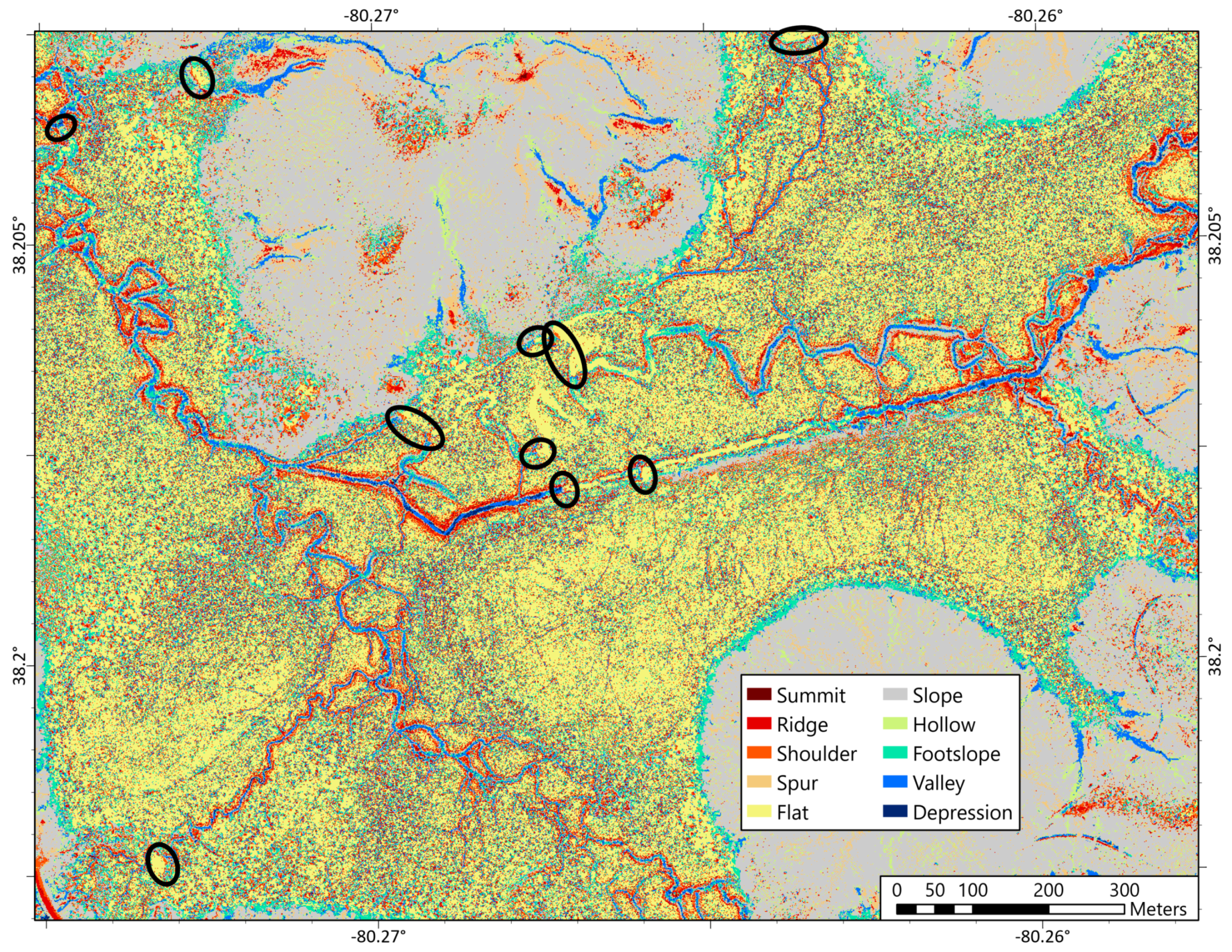
Supervised Maximum Likelihood landcover classification (Figure 9) that includes input from near-infrared channels (Figure 4) can outperform RGB-only classification thanks to the enhanced differentiation between waterlogged areas and adjacent dry surfaces. The landcover analysis presented here detects beaver impoundments while excluding free-flowing stretches, which in retrospect reinforced our identifications. Drawbacks included obscuring by overhanging vegetation and chronic misclassification of shadows with a 50/50 split between assignment to Needleleaf and Water.

3.8. Geomorphons

Geomorphon terrain analysis (Figure 10) reliably detects active impoundments, visible as noiseless Flat areas immediately upstream of each dam. This important feature of geomorphon-based impoundment detection is made possible by exploiting non-bathymetric Lidar’s tendency to fail at detecting laser returns from surfaces of water bodies [55,56]. These impoundments starkly interrupt their host stream’s vibrant Ridge-Valley-Ridge cross-sectional sequence, perhaps most clearly demonstrated along Cranberry River’s New Channel in the center of the study area. All these features conspire to combinations of microtopographic texture that are well-suited to geomorphon visualization, which works well by itself but even better when incorporated into this study’s general toolkit.

3.9. Spatiotemporal Distribution of Beaver Impoundments

In total, we identified 29 beaver impoundments from analyses of aerial data acquired between 1990 and 2020 (Figure 11), which for the study area’s 80 ha of suitable riparian habitat gives a minimum mean density of one impoundment per 2.8 ha.

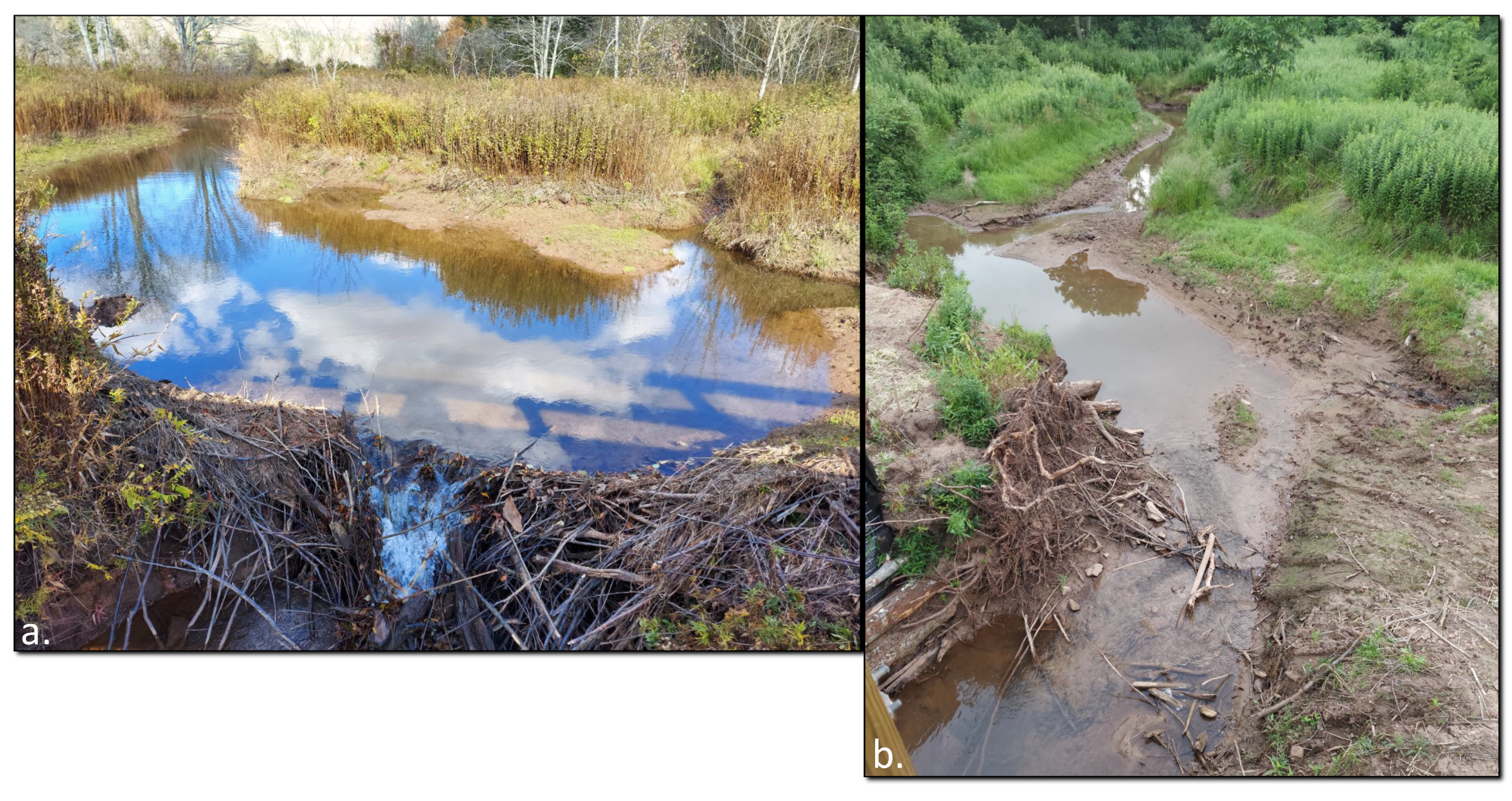
3.10. Site Validation

Ground-based repeat photography, an important component of our site validation process, not only documented seasonal (here, summer versus the previous fall) and hydrological dynamism but also offered important contextual clues for best interpretation of imagery detected from remote sensing platforms. Views of Charles Creek (38.191°, −80.264°; Figure 12) in October 2020 versus July 2021 show that the dam had been breached where it spanned the main channel, and vegetation was vigorously recolonizing the drained impoundment area. The lodge on the left was initially clearly visible but later became overgrown.

Another beaver-modified site along Charles Creek (38.192°, −80.265°; Figure 13) was just downstream of Figure 12 and photographed in October 2020 versus August 2021. In October, a full impoundment plus a human feature—Cow Pasture Trail—that has been co-opted as the primary spillway is visible. Charles Creek’s more deeply incised main channel sits just beyond the trail marker and is blocked along the indented portion of the dam. Ten months later, the dam was breached at the same point and the impoundment area reduced drastically. The nearly felled mature black cherry (Prunus serotina), displaying telltale bite gouges and hourglass tapering, stood testament to ongoing beaver activity in the vicinity.

Repeat photography of a beaver dam and impoundment along the upper Cranberry River (38.209°, −80.251°; Figure 14) showed a reversion to a free-flowing stream at some time between our visits. Initially there was an impoundment that had formerly pooled higher on the landscape, contained by a higher dam (inferred from the ‘bathtub ring’ of exposed mineral soil surrounding the impoundment up to a constant height). However, nine months later, the dam was breached and the impoundment had reverted to a pool-and-riffle stream type. The dam’s right flank had been converted to a low bank of mineral soil scored by tracks from heavy machinery during replacement of a footbridge along Cow Pasture Trail.

4. Discussion

Beaver have outsized roles as ecosystem engineers, making impacts that influence and intertwine with other key biophysical factors including climate change, local hydrological shifts, wildfires, and woody encroachment into imperiled peatlands such as the Cranberry Glades Botanical Area. They are, by nature, an expansionary keystone species and, through re-introductions, growing in number in both Europe and North America [13]. While beaver dams increase open water areas in valleys [59] and add numerous ecosystem services [60,61], they are also considered pests in some locations and contexts [10,11,12,13]. Monitoring of beaver activity, a potentially significant management tool for wetlands, may be best performed via remote sensing, given the difficulty of site access in remote areas and the potentially higher time commitment of field surveys.

Our study showed that several geospatial products from aerial imagery, including bare-earth model, canopy height model, hillshade, slope, true-color and color-infrared aerial photography, and supervised Maximum Likelihood classification, provided important information regarding the locations of beaver impoundments. However, each individual geospatial product also had limitations (Section 3.1, Section 3.2, Section 3.3, Section 3.4, Section 3.5, Section 3.6 and Section 3.7). These products were required to generate data for our geomorphon analysis, which in particular has proven to be an effective tool for locating beaver impoundments within the matrix of shrubby peatland ecotone enmeshing the heart of Cranberry Glades Botanical Area. Geomorphons successfully visualized all 10 impoundments that our analyses collectively detected from 2016 remotely sensed data. The success of geomorphon analysis is ironically related to its exploitation of absences and errors in both the Lidar data and the intermediate bare-earth model from which it was derived. It is unclear whether these flaws-turned-features would remain useful when applied to datasets of higher spatial quality.

A geomorphon analysis was invulnerable to the many drawbacks of illumination directionality that plagued our hillshade interpretation. Geomorphons highlighted the levees that bracketed most of the primary and secondary stream channels in the study area and revealed watertracks and game trails linking glade interiors with interglade beaver complexes. Furthermore, the zone in Big Glade first noted by Darlington as being actively eroded by Cranberry River’s New Channel in the early 1900s [41] was clearly highlighted by geomorphons. They also captured the relative landscape positions of most of the human transportation infrastructure such as the paved access road and wooden plank boardwalk in the southwest corner of the study area. Trails in the hills to the east also revealed their midslope cut-and-fill situations. Finally, geomorphons were resilient to binning artifacts, which arose during terrain model generation, that might otherwise require manual or algorithmic designation of breaklines along the edges of steeply incised stream channels [62].

We produced the most complete reconstruction of recent beaver activity across three recent decades at CGBA using a combination of aerial Lidar, aerial orthophotos, and repeat photography. In total, we identified 29 beaver impoundments from analyses of aerial data acquired between 1990 and 2020. These detected impoundments illustrate changing spatiotemporal patterns of beaver activity. We found more beaver impoundments during each 21st century decade than during the 1990s (18 vs. 13, respectively; Figure 15a), highlighting the possibility of population growth at Cranberry Glades. This would match the current tone of the literature indicating beaver expansion in many areas of the Northern Hemisphere [13]. The trend we detected was driven almost exclusively by activity in the main channels of our study zone (Charles Creek and Cranberry River by way of its New Channel). The persistence of detectable impoundments was most likely to fall into either one of the intermittent categories (one or two decades out of a possible three), while persistence throughout all three decades was much less likely to occur than either mode of intermittent persistence (Figure 15b). It is important to emphasize that substantial variations throughout these three decades—in the type, quality, and sampling frequency of aerial data—contributed additional bias to the probability of beaver impoundment detection, and this possibly detracts to some degree from our interpretation of spatiotemporal patterns.

Future research at this or other beaver-occupied sites could focus on hyperspectral imagery analysis and thereby improve classification accuracy of land cover, and more accurate classification of Lidar bare-earth returns could also be achieved using, for example, the Simple Morphological Filter [63]. Our strategy using publicly available imagery to identify present and past beaver impoundments could be useful for land managers or researchers looking to monitor beaver activity, to reconstruct past activity, or to model future changes to landscape. Estimating past beaver abundance through analyses of spatiotemporal change could provide baseline data for management consideration and may contribute useful insights for river basin restoration efforts.

References

1. Westbrook, C.J.; Cooper, D.J.; Baker, B.W. Beaver assisted river valley formation. River Res. Appl. 2011, 27, 247–256. [Google Scholar] [CrossRef]
2. Kuehn, R.; Schwab, G.; Schroeder, W.; Rottman, O. Differentiation of Castor fiber and Castor canadensis by noninvasive molecular methods. Zoo Biol. Publ. Affil. Am. Zoo Aquar. Assoc. 2000, 19, 511–515. [Google Scholar] [CrossRef]
3. Danilov, P.I.; Fedorov, F.V. Comparative characterization of the building activity of Canadian and European beavers in northern European Russia. Russ. J. Ecol. 2015, 46, 272–278. [Google Scholar] [CrossRef]
4. Gorczyca, E.; Krzemień, K.; Sobucki, M.; Jarzyna, K. Can beaver impact promote river renaturalization? The example of the Raba River, southern Poland. Sci. Total. Environ. 2018, 615, 1048–1060. [Google Scholar] [CrossRef] [PubMed]
5. Pollock, M.M.; Beechie, T.J.; Wheaton, J.M.; Jordan, C.E.; Bouwes, N.; Weber, N.; Volk, C. Using beaver dams to restore incised stream ecosystems. Bioscience 2014, 64, 279–290. [Google Scholar] [CrossRef]
6. Hood, G.A.; Larson, D.G. Ecological engineering and aquatic connectivity: A new perspective from beaver-modified wetlands. Freshw. Biol. 2015, 60, 198–208. [Google Scholar] [CrossRef]
7. Fairfax, E.; Whittle, A. Smokey the Beaver: Beaver-dammed riparian corridors stay green during wildfire throughout the western United States. Ecol. Appl. 2020, 30, e0225. [Google Scholar] [CrossRef]
8. Rozhkova-Timina, I.O.; Popkov, V.K.; Mitchell, P.J.; Kirpotin, S.N. Beavers as ecosystem engineers–A review of their positive and negative effects. IOP Conf. Ser. Earth Environ. Sci. 2018, 201, 012015. [Google Scholar] [CrossRef]
9. Wohl, E.; Dwire, K.; Sutfin, N.; Bazan, R. Mechanisms of carbon storage in mountainous headwater rivers. Nat. Commun. 2012, 3, 1–8. [Google Scholar] [CrossRef] [PubMed] [Green Version]
10. Butler, D.R.; Malanson, G.P. The geomorphic influences of beaver dams and failures of beaver dams. Geomorphology 2005, 71, 48–60. [Google Scholar] [CrossRef]
11. Green, K.C.; Westbrook, C.J. Changes in riparian area structure, channel hydraulics, and sediment yield following loss of beaver dams. J. Ecosyst. Manag. 2009, 10, 1. [Google Scholar]
12. Bailey, D.R.; Dittbrenner, B.J.; Yocom, K.P. Reintegrating the North American beaver (Castor canadensis) in the urban landscape. Wiley Interdiscip. Rev. Water 2019, 6, e1323. [Google Scholar] [CrossRef] [Green Version]
13. Brazier, R.E.; Puttock, A.; Graham, H.A.; Auster, R.E.; Davies, K.H.; Brown, C.M. Beaver: Nature’s ecosystem engineers. Wiley Interdiscip. Rev. Water 2020, 8, e1494. [Google Scholar] [CrossRef]
14. Graham, H.A.; Puttock, A.; Macfarlane, W.W.; Wheaton, J.M.; Gilbert, J.T.; Campbell-Palmer, R.; Elliott, M.; Gaywood, M.J.; Anderson, K.; Brazier, R.E. Modelling Eurasian beaver foraging habitat and dam suitability, for predicting the location and number of dams throughout catchments in Great Britain. Eur. J. Wildl. Res. 2020, 66.3, 1–18. [Google Scholar] [CrossRef]
15. Global Invasive Species Database. Available online: http://www.iucngisd.org/gisd/species.php?sc=981 (accessed on 30 September 2021).
16. IUCN Redlist. Available online: https://www.iucnredlist.org/search/list?query=Beaver (accessed on 30 September 2021).
17. Brackley, C.; Geographic, C. Current Beaver Range and Historical Commercial Trapping Areas. Map from Rethinking the Beaver. Available online: https://www.canadiangeographic.ca/article/rethinking-beaver (accessed on 30 September 2021).
18. Map from WorldAtlas’ Maps of West Virginia Webpage. Available online: https://www.worldatlas.com/maps/united-states/west-virginia (accessed on 30 September 2021).
19. Edens, D.L. Cranberry Glades, A Unique Series of Boreal Bogs in the Appalachian Mountains of West Virginia. In West Virginia and Appalachia: Selected Readings; Adkins, H.G., Ewing, S., Zimolzak, C.E., Eds.; Kendall/Hunt Publishing Company: Dubuque, Iowa, 1977; pp. 19–37. [Google Scholar]
20. Johnston, C.A.; Naiman, R.J. The use of a geographic information system to analyze long-term landscape alteration by beaver. Landsc. Ecol. 1990, 4, 5–19. [Google Scholar] [CrossRef]
21. Townsend, P.A.; Butler, D.R. Patterns of landscape use by beaver on the lower Roanoke River floodplain, North Carolina. Phys. Geogr. 1996, 17, 253–269. [Google Scholar] [CrossRef]
22. Cunningham, J.M.; Calhoun, A.J.; Glanz, W.E. Patterns of beaver colonization and wetland change in Acadia National Park. Northeast. Nat. 2006, 13, 583–596. [Google Scholar] [CrossRef]
23. Polvi, L.E.; Wohl, E. The beaver meadow complex revisited–the role of beavers in post-glacial floodplain development. Earth Surf. Process. Landforms 2012, 37, 332–346. [Google Scholar] [CrossRef]
24. Johnston, C.A. Fate of 150 year old beaver ponds in the Laurentian Great Lakes Region. Wetlands 2015, 35, 1013–1019. [Google Scholar] [CrossRef]
25. Pearl, C.A.; Adams, M.J.; Haggerty, P.K.; Urban, L. Using occupancy models to accommodate uncertainty in the interpretation of aerial photograph data: Status of beaver in Central Oregon, USA. Wildl. Soc. Bull. 2015, 39, 319–325. [Google Scholar] [CrossRef]
26. Puttock, A.K.; Cunliffe, A.M.; Anderson, K.; Brazier, R.E. Aerial photography collected with a multirotor drone reveals impact of Eurasian beaver reintroduction on ecosystem structure. J. Unmanned Veh. Syst. 2015, 3, 123–130. [Google Scholar] [CrossRef]
27. Levine, R. The Influence of Beaver Activity on Modern and Holocene Fluvial Landscape Dynamics in Southwestern Montana. Ph.D. Dissertation, The University of New Mexico, Albuquerque, NM, USA, 2016. [Google Scholar]
28. Briggs, M.A.; Wang, C.; Day-Lewis, F.D.; Williams, K.H.; Dong, W.; Lane, J.W. Return flows from beaver ponds enhance floodplain-to-river metals exchange in alluvial mountain catchments. Sci. Total Environ. 2019, 685, 357–369. [Google Scholar] [CrossRef] [PubMed] [Green Version]
29. Hood, G.A. Not all ponds are created equal: Long-term beaver (Castor canadensis) lodge occupancy in a heterogeneous landscape. Can. J. Zool. 2020, 98, 210–218. [Google Scholar] [CrossRef]
30. Karran, D.J.; Westbrook, C.J.; Wheaton, J.M.; Johnston, C.A.; Bedard-Haughn, A. Rapid surface-water volume estimations in beaver ponds. Hydrol. Earth Syst. Sci. 2017, 21, 1039–1050. [Google Scholar] [CrossRef] [Green Version]
31. Malison, R.L.; Lorang, M.S.; Whited, D.C.; Stanford, J.A. Beavers (Castor canadensis) influence habitat for juvenile salmon in a large Alaskan river floodplain. Freshw. Biol. 2014, 59, 1229–1246. [Google Scholar] [CrossRef]
32. Jasiewicz, J.; Stepinski, T.F. Geomorphons-A pattern recognition approach to classification and mapping of landforms. Geomorphology 2013, 182, 147–156. [Google Scholar] [CrossRef]
33. Melo, P.A.; Alvarenga, L.A.; Tomasella, J.; Mello, C.R.; Martins, M.A.; Coelho, G. Sensitivity and Performance Analyses of the Distributed Hydrology–Soil–Vegetation Model Using Geomorphons for Landform Mapping. Water 2021, 13, 2032. [Google Scholar] [CrossRef]
34. Gawrysiak, L.; Kociuba, W. Application of geomorphons for analysing changes in the morphology of a proglacial valley (case study: The Scott River, SW Svalbard). Geomorphology 2020, 371, 107449. [Google Scholar] [CrossRef]
35. Yan, G.; Cheng, H.; Teng, L.; Xu, W.; Jiang, Y.; Yang, G.; Zhou, Q. Analysis of the Use of Geomorphic Elements Mapping to Characterize Subaqueous Bedforms Using Multibeam Bathymetric Data in River System. Appl. Sci. 2020, 10, 7692. [Google Scholar] [CrossRef]
36. De Souza Robaina, L.E.; Trentin, R. Analysis of the basin of the Uruguay river through automated geomorphometric classification of the landforms elements. Rev. Bras. Geogr. FíSica 2018, 11, 2081–2093. [Google Scholar] [CrossRef] [Green Version]
37. Gioia, D.; Danese, M.; Corrado, G.; Di Leo, P.; Minervino Amodio, A.; Schiattarella, M. Assessing the Prediction Accuracy of Geomorphon-Based Automated Landform Classification: An Example from the Ionian Coastal Belt of Southern Italy. ISPRS Int. J. -Geo-Inf. 2021, 10, 725. [Google Scholar] [CrossRef]
38. Stine, M.B.; Resler, L.M.; Campbell, J.B. Ecotone characteristics of a southern Appalachian Mountain wetland. Catena 2011, 86, 57–65. [Google Scholar] [CrossRef]
39. Clel, D.T.; Freeouf, J.A.; Keys, J.E.; Nowacki, G.J.; Carpenter, C.A.; McNab, W.H. Ecological subregions: Sections and subsections for the conterminous United States. Gen. Tech. Rep. 2007, WO-76D, 76. [Google Scholar]
40. McNab, W.H.; Clel, D.T.; Freeouf, J.A.; Keys, J.E., Jr.; Nowacki, G.J.; Carpenter, C.A. Description of “Ecological subregions: Sections of the conterminous United States”. Gen. Tech. Rep. 2007, WO-76B, 76. [Google Scholar]
41. Darlington, H.C. Vegetation and substrate of Cranberry Glades, West Virginia. Bot. Gaz. 1943, 104, 371–393. [Google Scholar] [CrossRef]
42. Brooks, A.B. Forestry and wood industries. West Va. Geol. Econ. Surv. 1911, 5, 481. [Google Scholar]
43. Swank, W.C. Beaver Ecology and Management in West Virginia; Conservation Commission of West Virginia: Charleston, WV, USA, 1949; Volume 1.
44. Quick, R.H.; Mann, R.; Swank, W.C. Report on Beaver Habits Study Pittman-Robertson Project West Virginia; Conservation Commission of West Virginia: Charleston, WV, USA, 1941; 92p.
45. Edens, D.L. The Ecology and Succession of Cranberry Glades, West Virginia. Ph.D. Dissertation, North Carolina State University, Raleigh, NC, USA, 1973. [Google Scholar]
46. Bailey, R.W. Status of beaver in West Virginia. J. Wildl. Manag. 1954, 18, 184–190. [Google Scholar] [CrossRef]
47. Cameron, C.C.; Grosz, A.E. Peat Resources section of Mineral Resources of the Cranberry Wilderness Study Area, Webster and Pocahontas Counties, West Virginia. Geol. Surv. Bull. 1981, 1494, 40–45. [Google Scholar] [CrossRef] [Green Version]
48. Lidar Explorer Tool. Available online: https://www.usgs.gov/core-science-systems/ngp/3dep (accessed on 30 September 2021).
49. USGS Earth Explorer. Available online: https://earthexplorer.usgs.gov/ (accessed on 30 September 2021).
50. Luscombe, D.J.; Anderson, K.; Gatis, N.; Wetherelt, A.; Clement, E.G.; Brazier, R.E. What does airborne LiDAR really measure in upland ecosystems? Ecohydrology 2015, 8, 584–594. [Google Scholar] [CrossRef] [Green Version]
51. Gould, S.B.; Glenn, N.F.; Sankey, T.T.; McNamara, J.P. Influence of a dense, low-height shrub species on the accuracy of a Lidar-derived DEM. Photogramm. Eng. Remote Sens. 2013, 79.5, 421–431. [Google Scholar] [CrossRef]
52. Horn, B.K.P. Hill shading and the reflectance map. Proc. IEEE 1981, 69.1, 14–47. [Google Scholar] [CrossRef] [Green Version]
53. Pingel, T.J. Modeling slope as a contributor to route selection in mountainous areas. Cartogr. Geogr. Inf. Sci. 2010, 37, 137–148. [Google Scholar] [CrossRef] [Green Version]
54. Yokoyama, R.; Shirasawa, M.; Pike, R. Visualizing topography by openness: A new application of image processing to digital elevation models. Photogramm. Eng. Remote Sens. 2002, 68, 257–265. [Google Scholar]
55. Prošek, J.; Gdulová, K.; Barták, V.; Vojar, J.; Solský, M.; Rocchini, D.; Moudrý, V. Integration of hyperspectral and LiDAR data for mapping small water bodies. Int. J. Appl. Earth Obs. Geoinf. 2020, 92, 102181. [Google Scholar] [CrossRef]
56. Steuer, H.; Schäffler, U.; Gross, A. Detection of standing water bodies in Lidar-data. In Proceedings of the Earth Observations of Global Changes EOGC 2011 Conference, Technische Universitaet Muenchen, Munich, Germany, 15 April 2011. [Google Scholar]
57. Slagter, B.; Tsendbazar, N.-E.; Vollrath, A.; Reighe, J. Mapping wetland characteristics using temporally dense Sentinel-1 and Sentinel-2 data: A case study in the St. Lucia wetlands, South Africa. Int. J. Appl. Earth Obs. Geoinf. 2020, 86, 102009. [Google Scholar] [CrossRef]
58. USDA Farm Service Agency. Available online: https://www.fsa.usda.gov/programs-and-services/aerial-photography/imagery-programs/naip-imagery/ (accessed on 30 September 2021).
59. Hood, G.A.; Bayley, S.E. Beaver (Castor canadensis) mitigate the effects of climate on the area of open water in boreal wetlands in western Canada. Biol. Conserv. 2008, 141, 556–567. [Google Scholar] [CrossRef]
60. Johnston, C.A. 12. Beaver Wetlands. In Wetland Habitats of North America; University of California Press: Oakland, CA, USA, 2012; pp. 161–172. [Google Scholar] [CrossRef]
61. Thompson, S.; Vehkaoja, M.; Pellikka, J.; Nummi, P. Ecosystem services provided by beavers Castor spp. Mammal Rev. 2021, 51, 25–39. [Google Scholar] [CrossRef]
62. Liu, X. Airborne LiDAR for DEM generation: Some critical issues. Prog. Phys. Geogr. 2008, 32, 31–49. [Google Scholar] [CrossRef]
63. Pingel, T.J.; Clarke, K.C.; McBride, W.A. An improved simple morphological filter for the terrain classification of airborne LIDAR data. ISPRS J. Photogramm. Remote Sens. 2013, 77, 21–30. [Google Scholar] [CrossRef]
Figure 1. (a) Current North American range of C. canadensis including historical trading posts and trapping areas [17]. (b) Site location in Southern High Allegheny Mountains of West Virginia, USA (modified from [18]). (c) An anomalously broad, nearly level valley containing Cranberry Glades Botanical Area and surrounding peatlands near the headwaters of the Cranberry River; drainage is to the northwest and away from the precipitous drop southeast into the valley of the Greenbrier River. (d) The heart of the peatlands containing our study site and featuring the eponymous open glades (modified from [19]); beavers occupy the riparian corridors, and the blue arrows indicate the direction of stream flow.
Land 10 01333 g001
Figure 2. Boardwalk along a shrubby ecotone between Flag Glade and bog forest, October 2020. Note the small white tufts of cottongrass (Eriophorum virginicum) out in the open glade. Black Mountain, in the far background to the northeast, stands 400 m above the Cranberry Glades Botanical Area and is just one of many summits ringing the valley.
Land 10 01333 g002
Figure 3. Orthophoto of study site, Cranberry Glades WV, “true color” (RGB) channels, July 2018, NAIP.
Land 10 01333 g003
Figure 4. Orthophoto of study site, Cranberry Glades WV, “color infrared” (NRG) channels, July 2018, NAIP.
Land 10 01333 g004
Figure 5. Bare-earth model (BEM), December 2016, derived from USGS Lidar. The subtly domed glades also each tilt toward their collective centroid. The color scale was chosen to maximize visibility of along-channel discontinuities.
Land 10 01333 g005
Figure 6. Canopy Height Model (CHM), December 2016, derived from USGS Lidar. Circles indicate clearings within shrub belt (pale hues) along active watercourses, indicating possible beaver activity.
Land 10 01333 g006
Figure 7. Hillshade visualization, December 2016, derived from BEM in Figure 5. Light source azimuth and altitude 45°, vertical terrain exaggeration factor of two.
Land 10 01333 g007
Figure 8. Slope visualization, December 2016, derived from BEM in Figure 5. Red flags indicate three candidate beaver dam/impoundment complexes.
Land 10 01333 g008
Figure 9. Supervised Maximum Likelihood landcover classification derived from July 2018 NAIP multispectral aerial orthophotography. Broadleaf includes non-needleleaf trees and shrubs.
Land 10 01333 g009
Figure 10. Geomorphon landscape classification, Dec. 2016, derived from BEM (Figure 5). Ellipses highlight candidate beaver dams that support active impoundments, visible as noiseless Flat contiguous zones immediately upstream of each dam. The southernmost and second-northernmost dams were validated post hoc in addition to others within CGBA but exterior to this study site.
Land 10 01333 g010
Figure 11. Full remotely-detected census of beaver impoundments, 1990–2020, aggregated by decade (modified from [19]). Off-channel points represent impoundments either along unmapped tributaries, for example to the northwest, or along former channel routes that have since migrated laterally (e.g., those to the south and southwest).
Land 10 01333 g011
Figure 12. Beaver lodge, dam, and impoundment along Charles Creek (38.191°, −80.264°) in (a) October 2020 and (b) July 2021.
Land 10 01333 g012
Figure 13. Beaver impoundment along Charles Creek (38.192°, −80.265°) just downstream of Figure 12 in (a) October 2020 and (b) August 2021.
Land 10 01333 g013
Figure 14. Beaver dam and impoundment along Cranberry River where crossed by upper Cow Pasture Trail (38.209°, −80.251°) in (a) October 2020 reverting to free-flowing stream (b) by July 2021.
Land 10 01333 g014
Figure 15. (a) Individual beaver impoundments detected per decade, 1990–2020. Column values correspond to the number of times each instance is shown in Figure 11. (b) Persistence of detected beaver impoundments, 1990–2020. Subcategory values correspond directly to the number of instances of each in Figure 11.
Land 10 01333 g015
Publisher’s Note: MDPI stays neutral with regard to jurisdictional claims in published maps and institutional affiliations.