Integrated Land Use Change Related Carbon Source/Sink Examination in Jiangsu Province

Abstract

Carbon emission (CE) threatens global climate change severely, leading to the continuous strengthening of the greenhouse effect. Land use changes can greatly affect the ecosystem carbon budget and anthropogenic CE. Based on the land use grids, net ecosystem productivity (NEP), energy consumption-related CE, this study employed various methods to investigate the impact of land use change on carbon balance. The results showed 10.03% of total land use area has land use type changed between 2000 and 2015. Built-up land occupied cropland was the main land use transfer type. The period with the most intense land use changes was 2005–2010, which was constant with the process of China’s urbanization. NEP presented an overall increasing trend excluding built-up land and water areas. Temporally, CE showed an increasing trend in 2000–2015, especially in the industry sector. Spatially, areas with the high energy-related CE were mainly distributed in the south, which has a relatively high economic level. The land use intensity values of cities in Jiangsu all presented an overall increasing trend, which is related to the economic development and local endowment. Cities with higher land use intensity were usually accompanied with high CE, suppressing NEP growth. From 2000 to 2015, soil carbon storage reduced by 0.15 × 10⁸ t, vegetation carbon storage reduced by 0.04 × 10⁸ t, and CE reached 17.42 × 10⁸ t. Total CE caused by land use change reached 15.46 × 10⁸ t. The findings can make references for the low-carbon development from ecological land protection, strengthen land management, and optimize urban planning.

1. Introduction

To alleviate the enormous damage caused by CE to global climate change, more than 100 countries have proposed carbon neutrality goals. China has stated the dual carbon goal of reaching a carbon peak by 2030 [1] and achieving carbon neutrality by 2060 [2]. Reducing CE and achieving carbon neutrality are urgent for the development of most countries in the world [3]. In the context of global climate change, land use is an important topic in regional carbon cycling and sustainable science [4,5,6]. REDD + encourages countries in the global South to reorganize their land use and forest governance to reduce CE, this is very important for increasing carbon storage and CE reduction [7,8,9]. Land is a common carrier of the “natural-social” system, and land use change has an important influence on both the carbon budget of terrestrial ecosystems [10,11,12], and anthropogenic CE [13,14,15,16,17]. Land use change can affect the carbon storage through land use pattern change and land cover change, including soil carbon storage and vegetation carbon storage [18,19]. Vegetation, soil carbon accumulation capacity, and carbon source/sink capacity of different land use types are quite different [20]. In addition, there is a large difference in the carbon source/sink capacity between different land use intensities of the same land use type, such as a forest with a high surface biomass always has a higher carbon accumulation and carbon sink capacity than a forest with low biomass [21]. Moreover, changes in land use types and land use intensity can dramatically alter surface human activity intensity and anthropogenic CE [22,23]. For example, built-up land expansion may attract high-density industrial activities and cause high-intensity energy consumption [24]. Anthropogenic CE also widely exists in human activities on the surface of ecological land, such as agricultural and pastoral activities that also consume energy [19,25].

Urban always expands by occupying ecological land. Vegetation carbon reduction usually occurs through releasing carbon into the atmosphere by reducing vegetation photosynthesis and carbon absorption [26]. The impervious surface in urban areas can also block the amount absorbed by soil [27]. Sealed impervious ground can reduce the respiration and exchange of soil carbon between the soil and the atmosphere [28]. Ecological land, especially woodland, usually has higher biomass levels and higher carbon storage, the deforestation has always been a key cause of carbon loss. Different from vegetation, how soil carbon storage (SOC) changes caused by urban expansion has not been determined. There is research indicating that SOC levels in urban land may be higher than others [29], there are existing studies showing that impervious surfaces caused by urbanization can lead to sharp SOC losses [30,31]. With the rapid urbanization process, the intensity of human activities is often greater, and the land use change is the most intense [32,33], the study on carbon balance change caused by land use change in high-speed urbanization areas is more typical.

Terrestrial ecosystems not only can serve as carbon sinks, but also carbon sources, so they can significantly affect atmospheric carbon cycle [34]. Net Ecosystem Productivity (NEP) can usually be used to test whether the ecosystem exerts a carbon source effect or a carbon sink effect [35]. A positive NEP value indicates that it acts as a carbon sink and absorbs CE from the atmosphere, on the contrary, it plays a carbon source effect releasing CE into the atmosphere. Existing studies showed that in the past two decades, the global terrestrial ecosystem has played more of a role as a net sink [36,37]. Till now, there are still great uncertainties for NEP simulations [38,39], the accuracy of NEP still needs to be improved according to more and more field observations. For spatial anthropogenic CE, some scholars have carried out spatial distribution simulations of anthropogenic CE from built-up land using different data around the world, including population density, gross domestic product (GDP) level [40], night light data [41,42,43], etc.; the accuracy of spatial distribution has been improved. According to land use data and fields emissions survey data, a more accurate-CE map was generated with a resolution of 1 km [44], compared to the 10 km resolution of a global emission map from the Emissions Database for Global Atmospheric Research (EDGAR) dataset; the accuracy has much been improved, but due to data limitation, it cannot cover a long time series. The light data especially has been widely applied to simulate the spatial distribution of CE [45,46].

China has been experiencing a rapid urbanization process. Considering the industrial process and land use change, especially the rapid built-up land expansion and the occupation of a large area of ecological land, the growth rate is rapidly accelerated [15]. Yangtze River Delta is one of the major economic zones in China, which is located in the eastern coastal areas and is experiencing rapid urbanization. Domestic research on CE has been concentrated in these regions [47,48,49]. Existing studies mainly focus on the influence of land use change on carbon balance [50,51,52], and the perspective of urban morphology [53,54,55]. While previous studies focused on the CE effect of single land use type, carbon storage and CE effect are often discussed separately. It is urgent to study and analyze the multi-angle changes in land and their impacts on carbon balance such as carbon storage, carbon budget and anthropogenic CE. This study can discover which types of land use transfer will cause significant carbon storage losses and CE changes, which sectors and places have high-intensity energy CE, and how changes in land use intensity affect carbon balance. It can enrich the literature related to land use and carbon sources/sinks and provide reference for low-carbon land use. Jiangsu province, located along the eastern coast, is one of the most economically developed regions in China, and the core province in the Yangtze River Delta. In recent years, Jiangsu province has been experiencing rapid urbanization, promoting economic development greatly. Along with the high economic growth, population increase and energy consumption enhancing, the built-up land expansion and urban land use intensity have been increasing continually [56]. Dramatic land use changes will undoubtedly bring significant carbon balance. Thus, we selected this province as our study area.

This study can enrich carbon balance examination research from both the “natural–anthropogenic” aspects combining land use/land cover change, energy CE, NEP, land use intensity. We will also put forward substantive suggestions on how to restrict energy carbon output and optimize low-carbon land use. Details of this research include the following: (1) the carbon storage change caused by land use change; (2) the changes in NEP and CE; (3) land use intensity changes and its effect on carbon balance; (4) the temporal changes of carbon balance.

2. Material and Methods

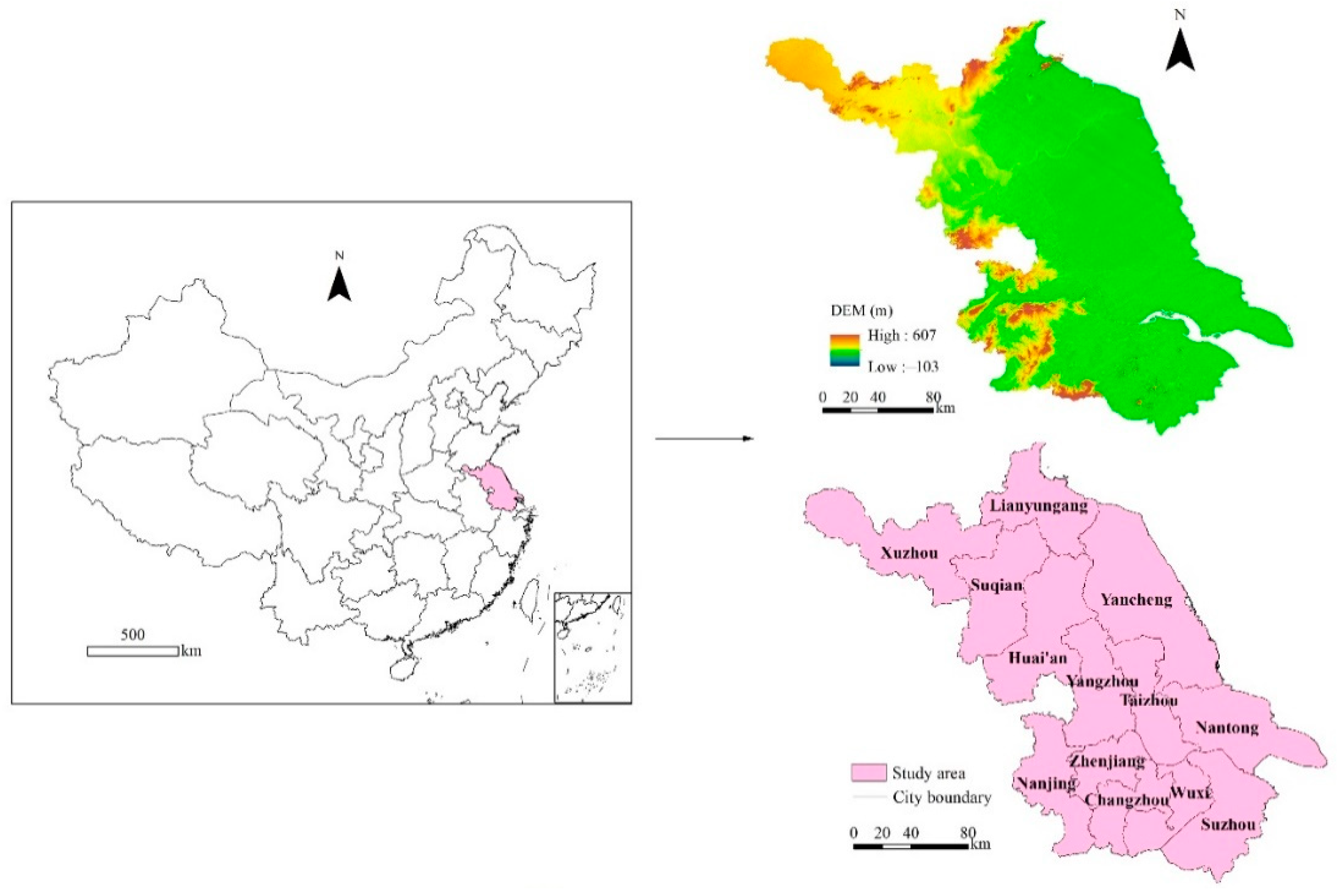
2.1. Study Area

Jiangsu province is located between latitudes 30°45′–35°2′ N and longitudes 116°18′–121°57′ E in the east of China (Figure 1). The topography is dominated by plains, accounting for 70% of the total area. The province has a typical monsoon climate, abundant precipitation, and excellent basic conditions for agriculture. These favorable natural conditions lay the foundation for social and economic development. This province hosts more than 80 million residents. The GDP of the province in 2020 ranked second in China, CNY 10.3 trillion, right behind Guangdong province. In recent years, rapid urbanization and industrialization led to obvious land use change [57], significantly affecting the regional carbon budget.

2.2. Data Sources

Data sources used in this study include energy consumption, night light data, land use grids, vegetation and soil carbon densities of different land use types, net primary productivity (NPP), climate data, DEM, and some economic data. (1) Energy consumption was obtained from the “China Energy Statistics Yearbook” for 2000–2015 and “Jiangsu Statistics Yearbook” for 2000–2015. (2) The DMSP/OLS night time stable light (NSL) data for 2000–2013 was obtained from the data archive and distribution system of the National Aeronautics and Space Administration (http://ladsweb.nascom.nasa.gov) (accessed on 17 March 2021). The NPP-VIIRS NSL data for 2014–2015 was obtained from the National Centers for Environmental Information website (https://www.ngdc.noaa.gov/eog/viirs/download_dnb_composites.html) (accessed on 17 March 2021). (3) The 30 × 30 m land use grids with a time series of 2000, 2005, 2010, and 2015 were provided by the Data Center for Resources and Environmental Sciences, Chinese Academy of Sciences (RESDC) (http://www.resdc.cn) (accessed on 17 March 2021), reclassified as six land use types, as cropland, forest, grassland, water area, built-up land, and unused land, respectively. (4) The vegetation and soil carbon densities of different land use types were referred to the study of Chuai et al. (2011) [58]. (5) For the NEP simulation, the annual MODIS NPP data from 2000 to 2015 used in this study were downloaded from the Numerical Terra-dynamic Simulation Group (NTSG) at the University of Montana (http://www.ntsg.umt.edu/) (accessed on 17 March 2021). Generally, the accuracy of the MODIS NPP products has been validated as being consistent with the field-observed NPP [59]. Meteorological data from 2000 to 2015 were observed at more than 2000 meteorological stations in China and mean annual precipitation and temperature values from each station were used. This data set was provided by the Data Center for Resources and Environmental Sciences, Chinese Academy of Sciences (RESDC) (http://www.resdc.cn) (accessed on 17 March 2021). The interpolation method used ANUSPLIN software [60] to generate precipitation and temperature grid maps to cover the whole area, and we extracted the Jiangsu grids from those across China. (6) Social and economic data was obtained from the “China Energy Statistics Yearbook” for 2000–2015 and “Jiangsu Statistics Yearbook” for 2000–2015.

2.3. Methods

2.3.1. CE Calculation

Based on the energy consumption data, using the CE coefficients of various energy sources determined by IPCC (2006), and referring to the study of Su et al. (2013) [46], nine major energy sources were selected to calculate CE. The formula is as follows:

$$C={\displaystyle \sum _{i=1}{K}_i}{E}_i$$

(1)

where, $i$ represents the type of energy; $K_i$ is the CE coefficient of energy $i$ (10⁴ tons of carbon)/(10⁴ t of standard coal); $E_i$ represents the consumption of energy $i$, calculated as standard coal (10⁴ t). The CE coefficients and conversion coefficients of standard coal for the nine energy sources are shown in

Table 1. CE coefficients of various energy types.

	Raw Coal	Coke	Crude	Gasoline	Kerosene	Diesel Fuel	Fuel Oil	Natural Gas	Electricity
Converted into standard coal (t standard coal/t)	0.7143	0.9714	1.4286	1.4714	1.4714	1.4571	1.4286	1.3300	0.3450
CE coefficient (104 t carbon/104 t standard coal)	0.7559	0.8550	0.5857	0.5538	0.5714	0.5921	0.6185	0.4483	0.2720

.

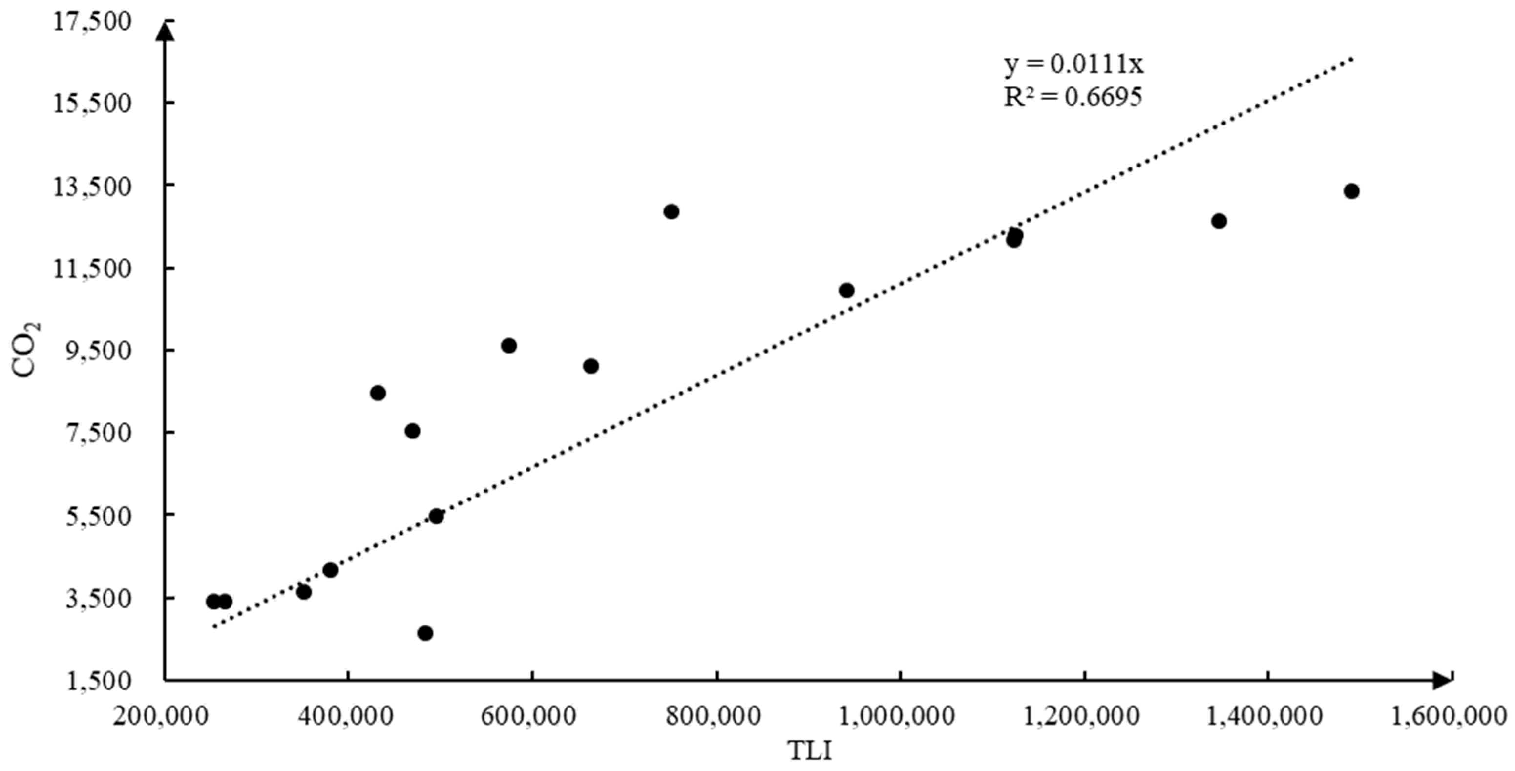
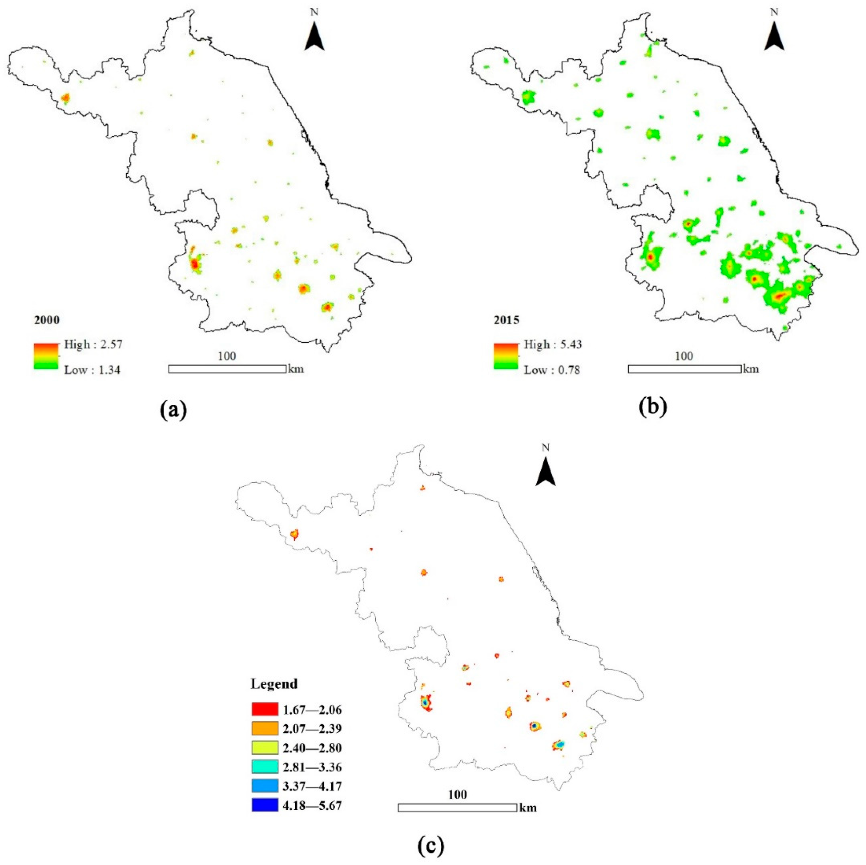
2.3.2. CE Spatialization

Before data processing, the monthly average data from January to December of 2014 and 2015 were synthesized into annual data through ENVI 5.1. NPP-VIIRS NSL data processing includes noise removal and continuity correction with DMSP/OLS night light data.

First, the DMSP/OLS night-time light data for 2013 was extracted as a dark background mask, and then the accidental noise in the NPP-VIIRS night-time light data of 2014 and 2015 was removed using this mask. Second, according to the study of Li (2018) [61], the DN value of NPP-VIIRS night-time light data is exponentially associated with the DN value of DMSP/OLS NSL data, thus, we obtained the corrected NPP-VIIRS NSL data of 2014 and 2015. The formula is as follows:

$$Y=a\ast X_b$$

(2)

After further processing, Equation (1) can be transformed into the following:

$$X=e^{\frac{\ln Y-\ln a}{b}}$$

(3)

where, $Y$ represents the DN value of DMSP/OLS NSL data, $X$ is the DN value of DMSP/OLS NSL data, and $a$ and $b$ are coefficients.

Then, the DMSP/OLS NSL data and NPP-VIIRS night-time light data were integrated together.

According to previous studies [45,46], the total night light index (TLI) correlated strongly with CE. $A$ quantitative analysis was performed on the total light index and CE, and a linear model with no intercept was established (Figure 2). The formula is as follows:

$$A_s=0.0111\times B$$

(4)

where, $A_s$ is the energy CE and $B$ is the total night light index.

2.3.3. Carbon Storage Loss Caused by Land Use Change

Land use change is an important driving factor affecting the carbon storage of terrestrial ecosystems. The carbon storage of terrestrial ecosystems mainly includes vegetation carbon storage and soil carbon storage. Land use change alters soil or vegetation carbon storage by changing vegetation types or land use patterns.

$$C_{ij}=(V_i-V_j)\times A_{ij}$$

(5)

where, $C_{ij}$ is the soil/vegetation carbon storage loss caused by the land use type $i$ transferred to land use type $j$. $V_i$ and $V_j$ are soil/vegetation carbon densities of land use type $i$ and $j$. $A_{ij}$ is the area of land use type $i$ transferred to land use type $j$.

2.3.4. NEP Simulation

$NEP$ is an important indicator in terrestrial ecosystems. $NEP$ can be regarded as the net carbon exchange between natural ecosystems and the atmosphere without considering disturbances [60], which can be obtained from $NPP$ by subtracting soil heterotrophic respiration ($Rh$). Values greater than zero or less than zero indicate whether an ecosystem plays a carbon sink or a carbon source effect [62,63]. The relevant formulas are as follows:

$$NEP=NPP-Rh$$

(6)

where, $NPP$ is the net primary productivity (gC.m⁻².yr⁻¹), $NEP$ is the net ecosystem productivity (gC.m⁻².yr⁻¹), and $Rh$ is the soil heterotrophic respiration (gC.m⁻².yr⁻¹).

$$Rh=0.4679\times Rs+114.42$$

(7)

where, $Rh$ is the soil heterotrophic respiration (gC.m⁻².yr⁻¹) and $Rs$ is the soil respiration (gC.m⁻².yr⁻¹).

According to the improve model of soil respiration proposed by Yu et al. (2010) [23], Rs can be obtained. The calculation formulas are as below:

$$R{s}_{\mathrm{month}}=(0.588+0.118\times SOC)\times e^{\ln (1.83}{}^{\times e^{-0.006\times T})\times T÷10}\times (P+2.972)÷(P+5.657)\times 30$$

(8)

$$R{s}_{\mathrm{annual}}={\displaystyle \sum _{i=1}^{12}R{s}_{month}}$$

(9)

where, $T$ is the mean monthly air temperature (℃), $P$ is the mean monthly precipitation (cm), and SOC is the topsoil (0–20 cm) organic carbon storage density (kgC.m⁻²), and $R{s}_{\mathrm{month}}$ and $R{s}_{\mathrm{annual}}$ are the monthly and annual soil respiration, respectively.

To analyze the changing trends of NEP between 2000 and 2015 from the grids level, the slope analysis was used for analysis. The formula is as follows:

$$slope=\frac{n\times {\displaystyle \sum _{i=1}^{n}i\times NE{P}_i-{\displaystyle \sum _{i=1}^{n}i{\displaystyle \sum _{i=1}^{n}NE{P}_i}}}}{n\times {\displaystyle \sum _{i=1}^n{i}^2-({\displaystyle \sum _{i=1}^{n}i{)}^2}}}$$

(10)

where $slope$ is the $NEP$ changing trend, $n$ is the number of studied time intervals (years), $NE{P}_i$ is the annual NEP for year $i$, and $slope$ > 0 and $slope$ < 0 represent increasing and decreasing tendencies of $NEP$, respectively.

2.3.5. Land Use Intensity Calculation

Index Selection

Humans can meet their own needs for land supply capacity through altering land use patterns and enhancing land use intensity, thus affecting the structure and function of ecosystems. Numerous studies have shown that land use intensity is associated with natural ecosystems closely [64]. Socioeconomic data can represent the situation of land use intensity to some extents. According to relevant research of Chuai et al. (2019) [38], we chose 8 indices to characterize land use intensity, presented in

Table 2. Main indices of the land use intensity description.

Comprehensive Index	Index	Affected Direction	Index Weight
Land use intensity	Urban population (X1)	+	0.09
	Average night light index (X2)	+	0.16
	GDP (X3)	+	0.18
	Agricultural output (X4)	+	0.18
	Shipment quantities (X5)	+	0.06
	Investment in fixed assets (X6)	+	0.16
	Industrial output (X7)	+	0.12
	Electricity consumption (X8)	+	0.04

, of urban population $X_1$, the average night light index $X_2$, GDP $X_3$, agricultural output $X_4$, shipment quantities $X_5$, investment in fixed assets $X_6$, industrial output $X_7$, and electricity consumption $X_8$ (Table 2).

Improved Entropy Method

The index weight can reflect the relative importance, which has an important influence on the accuracy and reliability of the results. During the practice of applying comprehensive evaluation methods, there are various evaluation methods. According to the different weighting methods, there are subjective weighting evaluation methods and objective weighting evaluation methods. This study employed the entropy method in the objective weighting method and determined the weight through the principle of information entropy, which can objectively and accurately evaluate the research object. In order to achieve the comparison between different years and different cities, this study improved the entropy method and added time variables to make the analysis results more reasonable. The improved entropy method evaluation model is as follows:

(1) Index selection: assuming that there are r years, n cities, and m indicators, then $x_{\theta ij}$ is the $j$-th indicator value of province $i$ in year θ.

(2) Data standardization: in order to eliminate the influence of the magnitude and dimensional differences of various indicators on the calculation results, the indicators were standardized to reduce random factors. In this study, the extreme value standardization method was used to normalize the index data. The specific formula is as follows:

$$x_{ij}^{\prime }=\frac{x_{ij}-\underset{i}{\min }\left\{x_{ij}\right\}}{\underset{i}{\max }\left\{x_{ij}\right\}-\underset{i}{\min }\left\{x_{ij}\right\}}(i=1, 2, \dots , \mathrm{m}; j=1, 2, \dots , \mathrm{n})$$

(11)

In the new data obtained through this standardization, the maximum value of each element is 1, the minimum value is 0, and the remaining values are between 0 and 1.

(3) Index weight determination:

$$y_{\theta ij}=\raisebox{1ex}{$x_{\theta ij}^{\prime }$}\!\left/ \!\raisebox{-1ex}{${\displaystyle \sum _{\theta }{\displaystyle \sum _i{x}_{\theta ij}^{\prime }}}$}\right.$$

(12)

(4) Calculate the entropy value of the $j$-th index:

$$e_j=-k{\displaystyle \sum _{\theta }{\displaystyle \sum _i{y}_{ij}\ln \left(y_{\theta ij}\right)}}$$

(13)

$$\mathrm{among} \mathrm{them}, k > 0,k=\frac{1}{\ln (rn)}$$

(14)

(5) Calculate the information utility value of the $j$-th indicator:

$$g_j=1-e_j$$

(15)

(6) Calculate the weight of each indicator:

$$w_j=\raisebox{1ex}{$g_j$}\!\left/ \!\raisebox{-1ex}{${\displaystyle \sum _j{g}_j}$}\right.$$

(16)

(7) Calculate the comprehensive score of each city’s land use intensity level:

$$H_{\theta i}={\displaystyle \sum _j{w}_j{x}_{\theta ij}}$$

(17)

3. Results

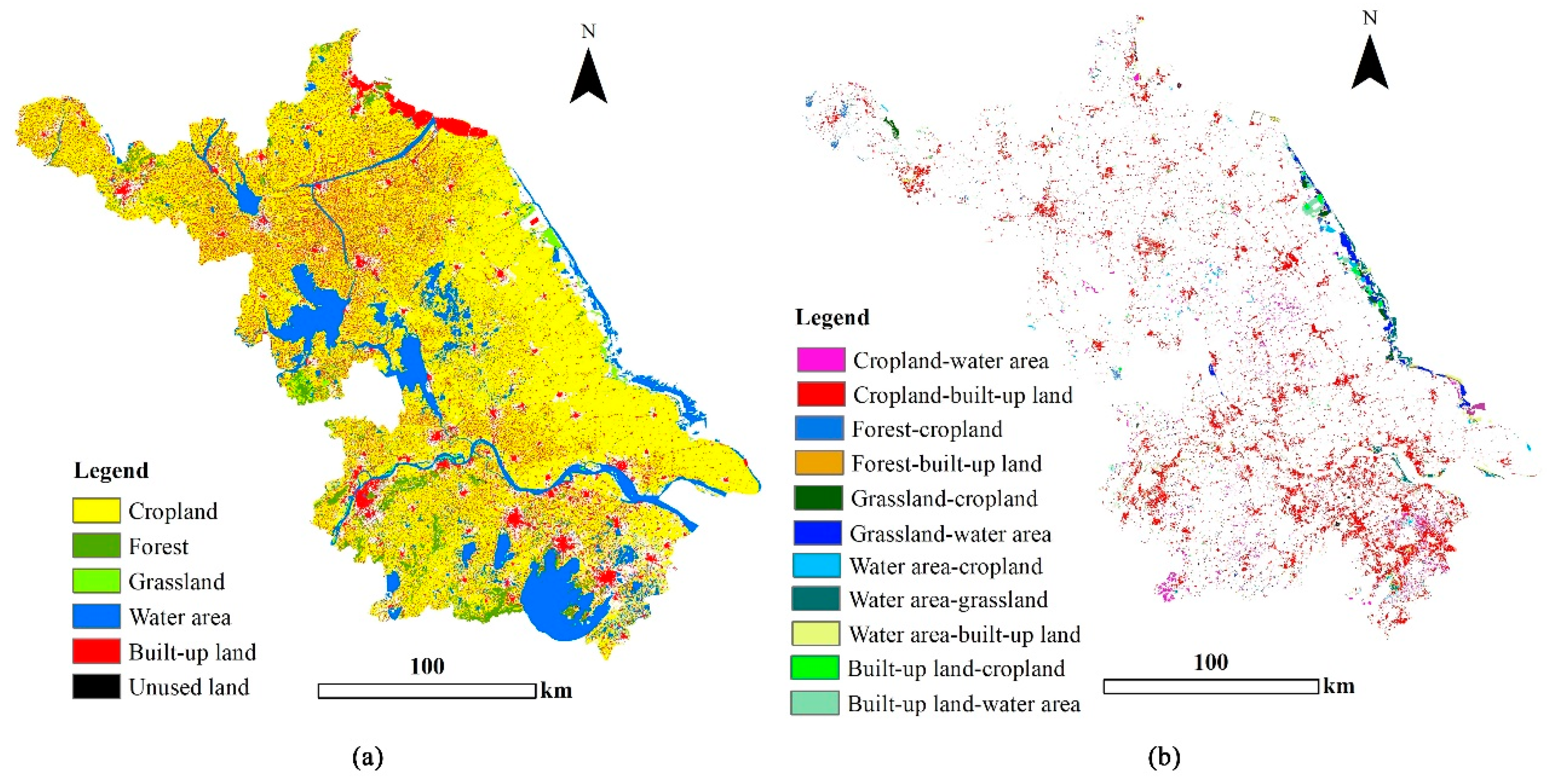
3.1. Changes in the Land Use Type and Carbon Storage

Between 2000 and 2015, the period of 2005–2010 presented the most obvious land use changes. Cropland was the main land use type of Jiangsu province, from 2000 to 2015, cropland decreased 6596.33 km², accounting for −9.45%. Forest also presented a decreasing trend. Grassland accounted for a small proportion, but showed a significant decreasing trend, its area decreased −398.87 km² from 2000 to 2015, accounting for −26.79%. Built-up land was the land use type with the most obvious increasing trend, its area increased 6497.01 km² from 2000 to 2015, accounting for 44.29%, especially in the period of 2005–2010 with 4388.82 km² increased. Water area decreased 728.85 km² in 2010–2015. Unused land presented a drastic increasing trend from 2000 to 2015 with 164.97 km², accounting for 903.83% of the total in 2000 (

Table 3. Land use area changes between typical years (km²).

Land Use Type	2000–2005	2005–2010	2010–2015	2000–2015
Cropland	−1220.07	−4594.22	−782.04	−6596.33
Forest	5.00	−260.76	−43.47	−299.23
Grassland	−86.60	−466.77	154.49	−398.87
Water area	307.79	1448.98	−728.85	1027.93
Built-up land	995.09	4388.82	1113.10	6497.01
Unused land	−1.22	198.61	−32.42	164.97
Changing rates
Cropland	−1.75%	−6.70%	−1.22%	−9.45%
Forest	0.15%	−7.70%	−1.39%	−8.85%
Grassland	−5.82%	−33.29%	16.52%	−26.79%
Water area	2.19%	10.08%	−4.61%	7.31%
Built-up land	6.78%	28.02%	5.55%	44.29%
Unused land	−6.68%	1166.07%	−15.04%	903.83%

).

Table 4. Land use and carbon storage transfer matrix between 2000 and 2015.

	Cropland	Forest	Grassland	Water Area	Built-Up Land	Unused Land	Total
Land use transfer matrix (km2)
Cropland	62,225.44	62.11	35.62	930.51	6493.81	33.14	69,780.64
Forest	197.00	3006.18	0.99	9.40	135.30	33.96	3382.82
Grassland	208.84	1.67	708.01	463.53	103.23	3.29	1488.57
Water area	232.30	1.42	288.45	12,974.58	378.73	82.10	13,957.58
Built-up land	317.91	10.72	32.43	285.90	14,007.94	13.19	14,668.09
Unused land	0.03	1.08	0.00	2.03	1.45	13.67	18.25
Total	63,181.53	3083.18	1065.49	14,665.96	21,120.45	179.35	103,295.95
Vegetation carbon storage transfer matrix (104 t)
Cropland	0.00	8.62	−1.22	−45.97	−351.96	−1.79	−392.32
Forest	−27.34	0.00	−0.17	−1.77	−26.11	−6.55	−61.94
Grassland	7.14	0.29	0.00	−7.05	−2.06	−0.07	−1.74
Water area	11.48	0.27	4.38	0.00	−1.82	−0.38	13.93
Built-up land	17.23	2.07	0.65	1.37	0.00	0.00	21.32
Unused land	0.00	0.21	0.00	0.01	0.00	0.00	0.22
Total	8.51	11.45	3.64	−53.40	−381.96	−8.78	−420.53
Soil carbon storage transfer matrix (104 t)
Cropland	0.00	21.37	2.42	−109.80	−1292.27	−6.06	−1384.35
Forest	−67.77	0.00	−0.27	−4.34	−73.47	−17.90	−163.74
Grassland	−14.20	0.46	0.00	−86.22	−27.56	−0.83	−128.35
Water area	27.41	0.66	53.65	0.00	−30.68	−5.34	45.70
Built-up land	63.26	5.82	8.66	23.16	0.00	0.21	101.11
Unused land	0.01	0.57	0.00	0.13	−0.02	0.00	0.68
Total	8.71	28.87	64.46	−177.07	−1424.00	−29.91	−1528.94

shows that there were obvious land use transfers in Jiangsu between 2000 and 2015. Cropland was the main exporter, mainly converted into built-up land and water area; built-up land was the main receiver, receiving a large amount of transfer from cropland, forest, grassland, and water area, increasing rapidly; besides water area, grassland mainly transferred into cropland and built-up land. The area of unused land was less, without obvious transfers. Overall, the drastic land use changes mainly include the following: first, the area of cropland converted into built-up land reached 6493.81 km², accounting for 9.31% of the total area of cropland in 2000, while, the area of built-up land converted into cropland was only 317.91 km², accounting for 2.17% of the total area of built-up land in 2000; second, the area of cropland transferred to water area was 930.51 km², accounting for 1.33% of the total area of cropland in 2000; third, the area of grassland transferred to water area was 463.53 km², accounting for 31.14% of the total area of grassland in 2000 (Table 4).

Based on the land use transfer matrix between 2000 and 2015, the carbon storage change caused by land use change can be obtained. The results only considered the change caused by land use type change, without considering change during the process of land use type change. The results showed, between 2000 and 2015, the carbon storage decreased 1949.47 × 10⁴ t, including 1949.47 × 10⁴ t of soil carbon storage and 420.53 × 10⁴ t of vegetation carbon storage. Land use changes led to the release of organic carbon. The transfer of cropland to built-up land reduced vegetation carbon storage by 351.96 × 10⁴ t and soil carbon storage by 1292.27 × 10⁴ t. The transfer of forest to cropland resulted in the reduction of vegetation carbon storage by 27.34 × 10⁴ t and soil carbon storage by 67.77 × 10⁴ t. The transfer of forest to built-up land led to 26.11 × 10⁴ t reduction in vegetation carbon storage, and 73.47 × 10⁴ t reduction in soil carbon storage (Table 4).

To better exhibit the spatial distribution of land use transfer, this study chose 11 typical land use transfer types, the total area of these 11 land use transfer types accounted for 95.87% of the total land use change area. Areas with larger land transfer patches were mainly distributed in the south and some northern core areas. The conversion of cropland into built-up land was the main land transfer type, accounting for 65.38% of the total area of 11 land use transfer types, which was mainly distributed in the south area. Cropland transfers were mainly distributed in the southeast and southwest areas, the central area also had sporadic distribution; the transfer of grassland to water area was mainly distributed in coastal areas; the transfer of built-up land to water was mainly distributed in the northeast edge area (Figure 3).

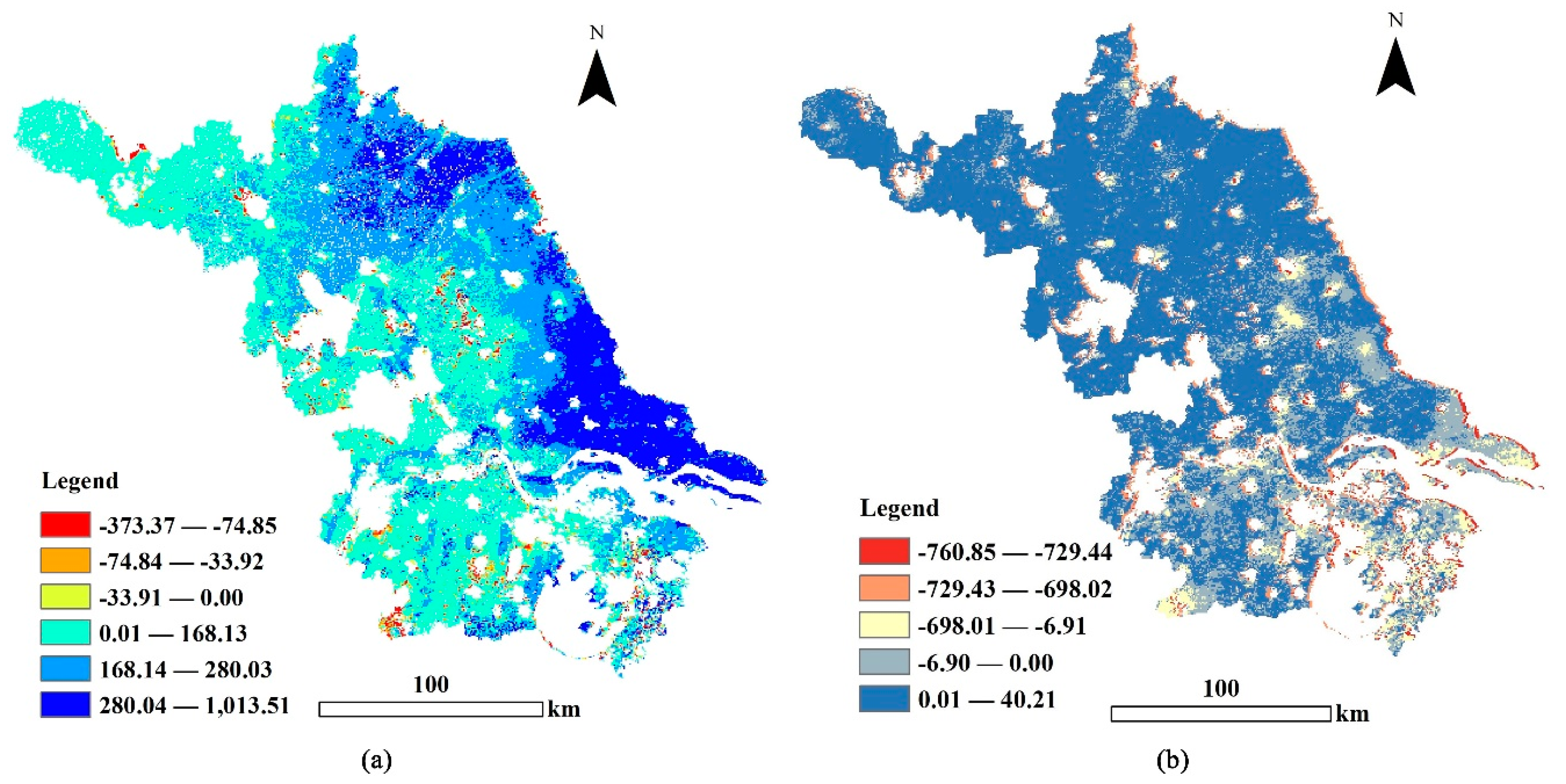
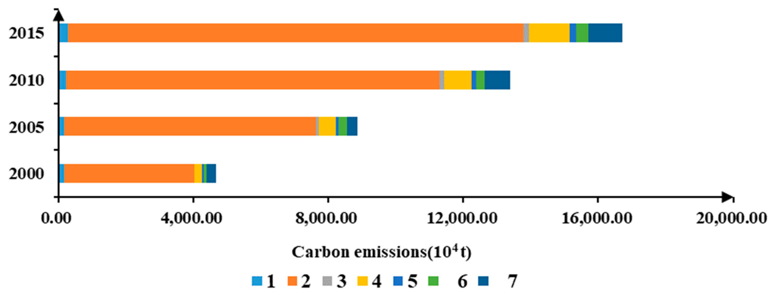
3.2. Changes in NEP and CE

Figure 4 shows the distributions of annual mean NEP and the changing trend between 2000 and 2015. The average annual NEP values ranged from −373.37 to 1013.51 gC.m⁻².yr⁻¹ between 2000 and 2015, and the mean NEP for the entire area was 172.16 gC.m⁻².yr⁻¹, which means it acts as a carbon sink. Grids with lower NEP values were mainly distributed in the surrounding water area and urban area. Grids with negative NEP values were mainly scattered in the part of the middle and south areas, which indicates that the ecosystem plays a role as a carbon source. Grids with positive NEP values were primarily located in most of the province, acting as carbon sinks. Grids with NEP values in the range of 0.01 to 168.13 gC.m⁻².yr⁻¹ were mainly distributed in the western part of the area, and grids with NEP values ranged from 280.04 to 1013.51 gC.m⁻².yr⁻¹ were mainly concentrated on the coast (Figure. 4a). The slope of NEP varied between −760.85 and 40.21 gC.m⁻².yr⁻¹. Grids with positive values were distributed in the largest area, indicating NEP presented an increasing trend. Grids with negative values were mainly scattered on the edge of water areas and built-up land (Figure 4b).

Figure 5 shows the spatial distribution of energy-related CE in 2000 and 2015, and the average annual values between 2000 and 2015. Energy-related CE intensities were densely distributed in the south area and presented an increasing trend, changing from a range of 1.34 × 10⁴ t.km⁻² to 2.57 × 10⁴ t.km⁻² in 2000 (Figure 5a) to a range of 0.78 × 10⁴ t.km⁻² to 5.43 × 10⁴ t.km⁻² in 2015 (Figure 4b). Mean annual energy-related CE intensities ranged between 1.67 × 10⁴ t.km⁻² and 5.67 × 10⁴ t.km⁻² from 2000 to 2015. Areas with values ranging between 1.67 × 10⁴ t.km⁻² and 2.80 × 10⁴ t.km⁻² were mainly located in parts of the north and southeast area. Areas with high values in a range of 2.81 × 10⁴ t.km⁻² to 5.67 × 10⁴ t.km⁻² were distributed in the part of the southwest area (Figure 5c).

Overall, CE presented an increasing trend, increasing from 4663.40 × 10⁴ t in 2000 to 16,712.35 × 10⁴ t in 2015. Figure 6 shows the changing trend in the various industries from 2000 to 2015. Specifically, the industry was the biggest contributor to the total CE, accounting for 82.50%, 84.17%, 82.79%, 80.76%. Transportation, warehousing, and postal industry was the secondary contributor, with an increasing trend from 4.28% in 2000 to 7.18% in 2015. Agriculture, forestry, animal husbandry, fishery, water conservancy, construction industry, wholesale, retail, accommodation, and catering, others, and living consumption all presented increasing trends. All these CE can be assigned to corresponding land use types.

Numbers 1–7 represent agriculture, forestry, animal husbandry, fishery, water conservancy; industry; construction industry; transportation, warehousing, postal industry; wholesale, retail, accommodation, and catering; others; living consumption.

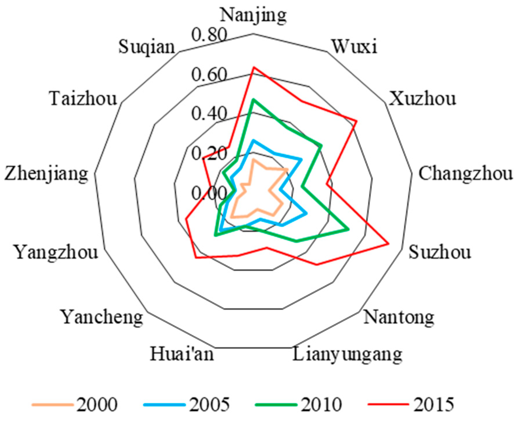
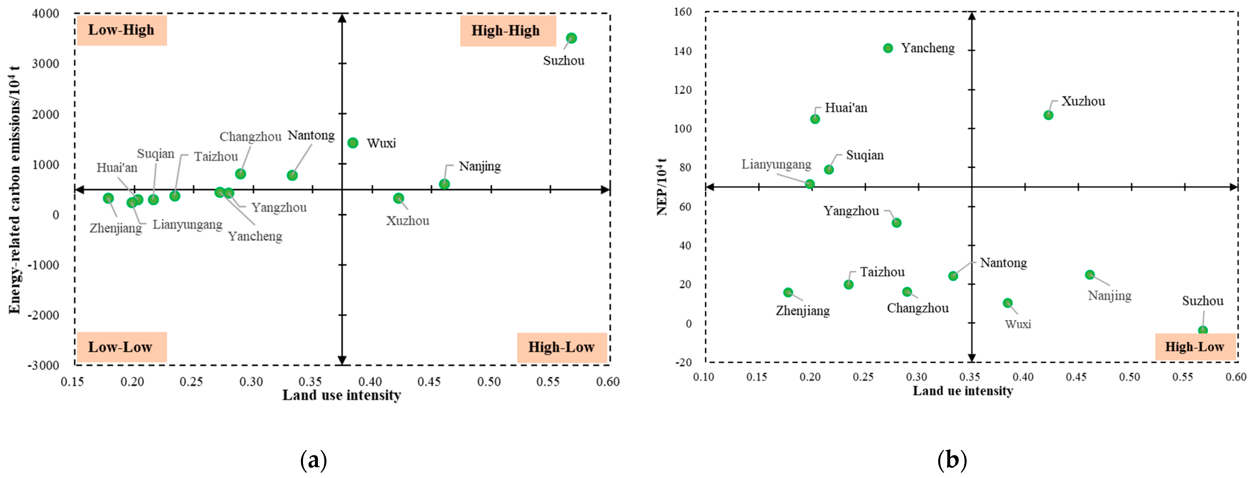
3.3. Changes in Land Use Intensity and Its Impact on Carbon Balance

Figure 7 shows that the land use intensity values of all cities presented similar increasing trends from 2000 to 2015. In 2000, the land use intensity values of all cities ranged between 0.038 and 0.209. Xuzhou had the highest land use intensity value, followed by Yancheng, Nantong, Suzhou, Wuxi, Nanjing, and Huai’an. After rapid economic development and urbanization process, Suzhou ranked the first with the highest land use intensity values in 2010 and 2015. Zhenjiang was always the city with the lowest land use intensity values, of 0.038, 0.089, 0.097, and 0.216 (Figure 7).

As shown above, land use intensity values increased to varying degrees. Then, how does the increase of land use intensity affect carbon balance? As the Figure 8 shows, land use intensity and energy-related CE, NEP showed a positive correlation and negative correlation relationships overall.

From the relationship between land use intensity change and energy-related CE change, most of the cities were concentrated in the third quadrant with low added value of land use intensity and low added value of energy-related CE, including Zhenjiang, Lianyungang, Yancheng, and Yangzhou. Nanjing, Wuxi, and Suzhou were located in the first quadrant, among which Suzhou had the highest land use intensity added value and CE added value, which were 0.57 and 3520.83 × 10⁴ t, respectively; Xuzhou was distributed in the fourth quadrant with a high added value of land use intensity, but low added value of energy-related CE (Figure 8a). From the relationship between land use intensity change and NEP change, the distribution of cities in the four quadrants was relatively balanced. Xuzhou was the only one located in the first quadrant with a high added value of land use intensity but a high NEP added value. Yancheng, distributed in the second quadrant, was the city with the highest value added of NEP. Corresponding to this, Suzhou was located in the first quadrant, with the lowest value added of NEP, −3.39 × 10⁴ t (Figure 8b).

3.4. Temporal Changes of Carbon Balance

We performed a comprehensive examination on the carbon sinks/sources in Jiangsu, calculated the total carbon storage and CE related to land use change. Due to the limitation of the land use grids, the changes of soil carbon storage and vegetation carbon storage were calculated at intervals of 5 years. From 2000 to 2015, soil carbon storage reduced by 0.15 × 10⁸ t, vegetation carbon storage reduced by 0.04 × 10⁸ t, and energy consumption CE was 17.42 × 10⁸ t. Total CE caused by land use changes reached 15.46 × 10⁸ t. CE showed an increasing trend, of 3.64 × 10⁸ t in 2000–2005, 6.06 × 10⁸ t in 2005–2010, and 7.71 × 10⁸ t in 2010–2015. The carbon sequestration capacity of NEP showed a fluctuating change and a phased decreasing trend, from 0.75 × 10⁸ t in 2000–2005 to 0.72 × 10⁸ t in 2005–2010 and 0.68 × 10⁴ t in 2010–2015, respectively. Soil and vegetation carbon storage decreased due to land use change, which played a carbon source role, with the largest reduction in 2005–2010, 0.11 × 10⁸ t in soil carbon storage reduction, and 0.03 × 10⁸ t in vegetation carbon storage reduction (

Table 5. Carbon balance change in 2000–2015 (10⁴ t).

Year	Soil Carbon Storage Loss	Vegetation Carbon Storage Loss	CE from Energy Consumption	NEP	Carbon Balance
2000	−0.02	−0.01	−0.47	0.08
2001			−0.47	0.15
2002			−0.50	0.14
2003			−0.57	0.12
2004			−0.76	0.16
2005			−0.88	0.10
2000–2005	−0.02	−0.01	−3.64	0.75	−2.92
2006	−0.11	−0.03	−1.00	0.15
2007			−1.13	0.14
2008			−1.25	0.17
2009			−1.35	0.12
2010			−1.34	0.14
2006–2010	−0.11	−0.03	−6.06	0.72	−5.48
2011	−0.02	−0.01	−1.39	0.10
2012			−1.43	0.16
2013			−1.57	0.14
2014			−1.66	0.13
2015			−1.67	0.15
2011–2015	−0.02	−0.01	−7.71	0.68	−7.06
2000–2015	−0.15	−0.04	−17.42	2.15	−15.46

).

4. Discussion and Policy Implications

For the analysis of land use change, built-up land occupied cropland was the main form in Jiangsu province, which is the universal phenomenon in China’s urbanization process [65]. Within the study area, the built-up land expansion in the south area was more obvious than that in the north area [66]. This is because the south area is the economic engine of the province with abundant resources, such as high-quality education, medical care, and highly developed commerce and industry, these factors will attract more people and require more built-up land to feed residents [57]. Moreover, considering the economic output benefit of land use, many croplands were converted into reservoir ponds in the coastal area [67]. During the critical period of rural revitalization, the government should reasonably guide urban-side industries to promote rural development [61], implement the balance of increase and decrease of urban and rural built-up land policy [68]. The period with most intense land use changes was 2005–2010. In recent years, the process of urbanization has slowed down, which is the general state of national urbanization development [69], land urbanization lags population increase, because population flow into urban areas seems to be much easier than building construction [70].

Urban areas have high population density and frequent human activities. It is reported that 2% of the world’s urban land accommodates more than 50% of the world’s population and emits about 75% of the world’s CE [51,71]. The rapid urban expansion will bring resource agglomeration, industrial development, energy consumption, and a large number of environmental problems [72]. In addition, the occupation of the surrounding cropland, forest, and other ecological land by urban expansion can release carbon into the atmosphere by reducing the light and function of vegetation [26], and finally, result in the increase in CE and decrease in carbon storage [56]. Increasing the rate of green space in urban areas seems to be an effective way to offset carbon losses [73]. Forest is a land-use type with the highest biomass and the highest vegetation carbon density. More vegetation with higher biomass should be planted in central urban areas, which can promote the biodiversity of ecosystems, activate soil biological activities, and increase soil fertility [43,74,75], thus increasing carbon storage. Land managers should take seriously consideration of environmental impact and urban green development when making land-use policies.

During rapid economic development, changes in CE intensity and NEP are substantial, both spatially and temporally. First, this study corrected and integrated the two types of NSL data from different sources, the reliability can be validated by the existing study [61]. Relevant studies have proved that NSL data can simulate CE well, using both the DMSP/OLS and NPP-VIIRS data [76,77]. Spatial changes in CE were more widely and densely distributed in the south. Resource consumption, an increase of industry intensity was the main reason for the increase in energy-related CE [78,79]. The backwardness of production technologies such as combustion and industry, fossil fuels, is another major reason for CE [80]. NEP are representative indicators that can present the carbon sinks capacity of vegetation growth. The NEP simulation used the latest soil survey data, using models based on field observations in China. Applications across China show that the simulated NEP can be well validated by field observations with high accuracy [81]. According to our results, except for downtown areas, some areas, such in the south and middle, displayed a decreasing trend in NEP, which may be partly caused by an expansion in water areas for aquaculture and urban expansion. Some areas that did not experience land transfer also showed a decrease in NEP, which should alert the attention of relevant departments, so that they can take effective measures to alleviate land degradation [81]. A certain degree of land management intervention can not only optimize land-use, but also affect ecosystem carbon balance [82,83]. Overall, the NEP reflects the predominant carbon sink capacity of terrestrial ecosystems, which was mainly attributed to the stable climate and good hydrothermal conditions in Jiangsu province [38].

Jiangsu province has experienced rapid urbanization in recent years, causing the land-use intensity to enhance rapidly [38]. Land-use intensity presented a descending trend from the south to the north overall [84], which was consistent with the previous study by Yang et al. (2018) [85], who demonstrated that land-use intensity increased with the improvement of urbanization level. Areas where land-use intensity has an obvious enhancing trend always have large percentages of artificial vegetation and land [86], which can also explain the lower NEP value [87]. The areas with greater natural and semi-natural land-use usually have lower land-use intensity [50], such as areas with large parts of cropland, forests, and grassland. This can also explain Xuzhou, which has high land-use intensity, while high NEP and low CE. Adjusting the energy structure, introducing green production technology will play important roles in reducing CE, and promote the sustainable development of cities. As more built-up land occupies ecological land, policies and measures for promoting intensive land-use should be carried out to adjust land-use intensity; this should be matched with the local socio-economic condition [88]. In addition, social-economic circumstances, climate change [89], ecological conditions, and crop plant structure all can affect land-use intensity to some extent.

For the examination of carbon balance, this study discussed the multi-angle changes of land use change, land-use type, and land-use intensity, and their impacts on carbon balance such as carbon storage, carbon sequestration, and anthropogenic CE. It comprehensively considers both natural and anthropogenic aspects. However, there are still some uncertainties in this study. Firstly, the calculation of energy CE is mainly based on the IPCC coefficient method [90], the coefficients used internationally may not be suitable for use in China, and there are certain errors. Second, the soil carbon densities and vegetation carbon densities of different land-use types in this study were regarded as constant values due to the data limitation and the property that carbon density change needs to take a long time. Third, due to data constraints, NEP spatial accuracy at the urban level may be relatively rough, which may lead to a certain deviation in the NEP test.

5. Conclusions

Land use changes have a significant impact on the carbon storage of terrestrial ecosystems and anthropogenic CE. This study found that about 10.03% of total land use area has experienced land use type change between 2000 and 2015. Built-up land occupied cropland was the main land use transfer type, accounting for 62.68% of the land use change area. Besides the impact on carbon balance, the reduction of cropland will also pose a threat to food security. Cities with higher land use intensity were usually accompanied with high CE of energy consumption, suppressing NEP growth. NEP presented an overall increasing trend excluding built-up land and water area, the total NEP was decreasing year by year, which is the combined impact of human activities and climate change. Planting trees with high biomass in the urban green area is the best way to increase carbon storage. In the future, we will focus on finely simulating the urban spatial changes and the impact on carbon balance of natural resources to achieve the goal of carbon neutrality.

References

1. Xi, J.P. Speech at the General Debate of the 75th Session of the United Nations General Assembly; State Council of the People’s Republic of China: Beijing, China, 2020.
2. Xinhua Net. Xi Jinping’s Speech at the Climate Ambition Summit. (12 September 2020) [15 October 2021]. Available online: http://www.xinhuanet.com/politics/leaders/2020-12/12/c_1126853599.htm (accessed on 22 November 2021).
3. Hasegawa, T.; Fujimori, S.; Frank, S.; Humpenoder, F.; Bertram, C.; Despres, J.; Drouet, L.; Emmerling, J.; Gusti, M.; Harmsen, M.; et al. Land-based implications of early climate actions without global net-negative emissions. Nat. Sustain. 2021, 909. [Google Scholar] [CrossRef]
4. Foley, J.A.; Defries, R.; Asner, G.P.; Barford, C.; Bonan, G.; Carpenter, S.R.; Chapin, F.S.; Coe, M.T.; Daily, G.C.; Gibbs, H.K.; et al. Global consequences of land use. Science 2005, 309, 570–573. [Google Scholar] [CrossRef] [Green Version]
5. Rockstrom, J.; Steffen, W.; Noone, K.; Persson, A.; Chapin, F.S.; Lambin, E.F.; Lenton, T.M.; Scheffer, M.; Folke, C.; Schellnhuber, H.J.; et al. A safe operating space for humanity. Nature 2009, 461, 472–475. [Google Scholar] [CrossRef]
6. Shevliakova, E.; Pacala, S.W.; Malyshev, S.; Hurtt, G.C.; Milly, P.C.D.; Caspersen, J.P.; Sentman, L.T.; Fisk, J.P.; Wirth, C.; Crevoisier, C. Carbon cycling under 300 years of land use change: Importance of the secondary vegetation sink. Glob. Biogeochem. Cycles 2009, 23, 2022. [Google Scholar] [CrossRef]
7. Irawan, S.; Tacconi, L.; Ring, I. Stakeholders’ incentives for land-use change and REDD+: The case of Indonesia. Ecol. Econ. 2013, 87, 75–83. [Google Scholar] [CrossRef]
8. Corbera, E.; Martin, A.; Springate-Baginski, O.; Villasenor, A. Sowing the seeds of sustainable rural livelihoods? An assessment of Participatory Forest Management through REDD+ in Tanzania. Land Use Policy 2020, 97, 102962. [Google Scholar] [CrossRef] [Green Version]
9. Sanders, A.J.P.; Ford, R.M.; Keenan, R.J.; Larson, A.M. Learning through practice? Learning from the REDD plus demonstration project, Kalimantan Forests and Climate Partnership (KFCP) in Indonesia. Land Use Policy 2020, 91, 104285. [Google Scholar] [CrossRef]
10. Potter, C.S.; Randerson, J. Terresrial ecosystem production: A process model based on global satellite and surface data. Glob. Biogeochem. Cycles 1993, 7, 811–842. [Google Scholar] [CrossRef]
11. Houghton, R.A.; Hackler, J.L.; Lawrence, K.T. The U.S. carbon budget: Contributions from land-Use change. Science 1999, 285, 574–578. [Google Scholar] [CrossRef] [PubMed]
12. Popp, A.; Krause, M.; Dietrich, J.P.; Lotze-Campen, H.; Leimbach, M.; Beringer, T.; Bauer, N. Additional CO2 emissions from land use change-forest conservation as a precondition for sustainable production of second generation bioenergy. Ecol. Econ. 2012, 74, 64–70. [Google Scholar] [CrossRef]
13. Houghton, R.A. Revised estimates of the annual net flux of carbon to the atmosphere from changes in land use and land management 1850–2000. Tellus Ser. B-Chem. Phys. Meteorol. 2003, 55, 378–390. [Google Scholar]
14. Houghton, R.A.; House, J.I.; Pongratz, J.; van der Werf, G.R.; DeFries, R.S.; Hansen, M.C.; Le Quere, C.; Ramankutty, N. Carbon emission from land use and land-cover change. Biogeosciences 2012, 9, 5125–5142. [Google Scholar] [CrossRef] [Green Version]
15. Chuai, X.W.; Huang, X.J.; Wang, W.J.; Zhao, R.Q.; Zhang, M.; Wu, C.Y. Land use, total carbon emission change and low carbon land management in Coastal Jiangsu, China. J. Clean. Prod. 2015, 103, 77–86. [Google Scholar] [CrossRef]
16. Erb, K.H.; Fetzel, T.; Plutzar, C.; Kastner, T.; Lauk, C.; Mayer, A.; Niedertscheider, M.; Körner, C.; Haberl, H. Biomass turnover time in terrestrial ecosystems halved by land use. Nat. Geosci. 2016, 9, 674–678. [Google Scholar] [CrossRef]
17. Li, Z.G.; Zhong, J.L.; Sun, Z.S.; Yang, W.N. Spatial pattern of carbon sequestration and urban sustainability: Analysis of land-use and carbon emission in Guang’an, China. Sustainability 2017, 9, 1951. [Google Scholar] [CrossRef] [Green Version]
18. Zhang, P.Y.; Li, y.y.; Jing, W.L.; Yang, D.; Zhang, Y.; Liu, Y.; Geng, W.L.; Rong, T.Q.; Shao, J.W.; Yang, J.X.; et al. Comprehensive assessment of the effect of urban built-up land expansion and climate change on net primary productivity. Complexity. 2020, 2020, 8489025. [Google Scholar] [CrossRef]
19. Qu, J.S.; Zeng, J.J.; Li, Y.; Wang, Q.; Maraseni, T.; Zhang, L.H.; Zhang, Z.Q.; Clarke Sather, A. Household carbon dioxide emissions from peasants and herdsmen in north-western arid-alpine regions, China. Energy Policy 2013, 57, 133–140. [Google Scholar] [CrossRef]
20. Zhang, P.Y.; He, J.J.; Hong, X.; Zhang, W.; Cheng, Z.Q.; Pang, B.; Li, Y.Y.; Liu, Y. Carbon sources/sinks analysis of land use changes in China based on data envelopment analysis. J. Clean. Prod. 2018, 204, 702–711. [Google Scholar] [CrossRef]
21. Lai, L.; Huang, X.J.; Yang, H.; Chuai, X.W.; Zhang, M.; Zhong, T.Y.; Chen, Z.G.; Chen, Y.; Wang, X.; Thompson, J.R. CE from land-use change and management in China between 1990 and 2010. Sci. Adv. 2016, 2, e1601063. [Google Scholar] [CrossRef] [Green Version]
22. Qu, J.S.; Maraseni, T.; Liu, L.N.; Zhang, Z.Q.; Yusaf, T. A comparison of household carbon emission patterns of urban and Rural China over the 17 year period (1995–2011). Energies 2015, 8, 10537–10557. [Google Scholar] [CrossRef]
23. Maraseni, T.N.; Qu, J.S.; Zeng, J.J. A comparison of trends and magnitudes of household carbon emission between China, Canada and UK. Environ. Dev. 2015, 15, 103–119. [Google Scholar] [CrossRef]
24. Tubiello, F.N.; Salvatore, M.; Rossi, S.; Ferrara, A.; Fitton, N.; Smith, P. The FAOSTAT database of greenhouse gas emissions from agriculture. Environ. Res. Lett. 2013, 8, 015009. [Google Scholar] [CrossRef]
25. Rong, T.Q.; Zhang, P.y.; Jing, W.L.; Zhang, y.; Li, Y.Y.; Yang, D.; Yang, J.X.; Chang, H.; Ge, L.N. Carbon dioxide emissions and their driving forces of land use change based on economic contributive coefficient (ecc) and ecological support coefficient (esc) in the lower yellow river region (1995–2018). Energies 2020, 13, 2600. [Google Scholar] [CrossRef]
26. Smith, S.J.; Rothwell, A. Carbon density and anthropogenic land-use influences on net land-use change emissions. Biogeosciences 2013, 10, 6323–6337. [Google Scholar] [CrossRef] [Green Version]
27. Castillo, J.A.A.; Apan, A.A.; Maraseni, T.N.; Salmo, S.G., III. Estimation and mapping of above-ground biomass of mangrove forests and their replacement land uses in the Philippines using Sentinel imagery. ISPRS J. Photogramm. Remote. Sens. 2017, 134, 70–85. [Google Scholar] [CrossRef]
28. Apan, A.; Suarez, L.A.; Maraseni, T.; Castillo, J.A. The rate, extent and spatial predictors of forest loss (2000–2012) in the terrestrial protected areas of the Philippines. Appl. Geogr. 2017, 81, 32–42. [Google Scholar] [CrossRef]
29. Chuai, X.W.; Huang, X.J.; Wang, W.J.; Zhang, M.; Lai, L.; Liao, Q.L. Spatial variability of soil organic carbon and comprehensive analysis of related factors in Jiangsu Province, China. Pedosphere 2012, 22, 404–414. [Google Scholar] [CrossRef]
30. Beesley, L. Carbon storage and fluxes in existing and newly created urban soils. J. Environ. Manag. 2012, 104, 158–165. [Google Scholar] [CrossRef]
31. Chen, J.L.; Gao, J.L.; Yuan, F.; Wei, Y.D. Spatial determinants of urban land expansion in globalizing Nanjing, China. Sustainability 2016, 8, 868. [Google Scholar] [CrossRef] [Green Version]
32. Weber, C.; Puissant, A. Urbanization pressure and modelling of urban growth: Example of the Tunis Metropolitan Area. Remote Sens. Environ. 2003, 86, 341–352. [Google Scholar] [CrossRef]
33. Houghton, R.A. The worldwide extent of land—Use change. BioScience 1994, 44, 305–313. [Google Scholar] [CrossRef]
34. Keenan, T.F.; Prentice, I.C.; Canadell, J.G.; Williams, C.A.; Wang, H.; Raupach, M.; Collatz, G.J. Recent pause in the growth rate of atmospheric CO2 due to enhanced terrestrial carbon uptake. Nat. Commun. 2016, 7, 13428. [Google Scholar] [CrossRef] [PubMed] [Green Version]
35. Grant, D.D.; Baldocchi, S.M. Ecological controls on net ecosystem productivity of a seasonally dry annual grassland under current and future climates: Modelling with ecosys. Agric. For. Meteorol. 2012, 152, 189–200. [Google Scholar] [CrossRef]
36. Dalal, R.C.; Allen, D.E. Greenhouse gas fluxes from natural ecosystems. Aust. J. Bot. 2008, 56, 369–407. [Google Scholar] [CrossRef]
37. Jones, C.; McConnell, C.; Coleman, K.; Cox, P.; Falloon, P.; Jenkinson, D.; Powlson, D. Global climate change and soil carbon stocks; predictions from two contrasting models for the turnover of organic carbon in soil. Glob. Chang. Biol. 2005, 11, 154–166. [Google Scholar] [CrossRef]
38. Chuai, X.W.; Yuan, Y.; Zhang, X.Y.; Guo, X.M.; Zhang, X.L.; Xie, F.J.; Zhao, R.Q.; Li, J.B. Multi-angle land use-linked carbon balance examination in Nanjing City, China. Land Use Policy 2019, 84, 305–315. [Google Scholar] [CrossRef]
39. Yu, G.R.; Zheng, Z.M.; Wang, Q.F.; Fu, Y.L.; Zhuang, J.; Sun, X.M.; Wang, Y.S. Spatiotemporal pattern of soil respiration of terrestrial ecosystems in China: The development of a geostatistical model and its simulation. Environ. Sci. Technol. 2010, 44, 6074–6080. [Google Scholar] [CrossRef]
40. Olivier, J.G.; van Aardenne, J.A.; Dentener, F.J.; Pagliari, V.; Ganzeveld, L.N.; Peters, J.A.H.W. Recent trends in global greenhouse gas emissions: Regional trends 1970−2000 and spatial distribution of key sources in 2000. Environ. Sci. 2005, 2, 81–99. [Google Scholar] [CrossRef] [Green Version]
41. Oda, T.; Maksyutov, S. A very high-resolution global fossil fuel CO2 emission inventory derived using a point source database and satellite observations of nighttime lights, 1980–2007. Atmos. Chem. Phys. 2010, 10, 16307–16344. [Google Scholar]
42. Doll, C.N.H.; Muller, J.P.; Elvidge, C.D. Night-time imagery as a tool for global mapping of socioeconomic parameters and greenhouse gas emissions. Ambio 2000, 29, 157–162. [Google Scholar] [CrossRef]
43. Rader, R.; Bartomeus, I.; Tylianakis, J.M.; Laliberte, E. The winners and losers of land use intensification: Pollinator community disassembly is non-random and alters functional diversity. Divers. Distrib. 2014, 20, 908–917. [Google Scholar] [CrossRef] [Green Version]
44. Wang, J.N.; Cai, B.F.; Zhang, L.X.; Cao, D.; Liu, L.C.; Zhou, Y.; Zhang, Z.S.; Xue, W.B. High Resolution Carbon Dioxide Emission Gridded Data for China Derived from Point Sources. Environ. Sci. Technol. 2014, 48, 7085–7093. [Google Scholar] [CrossRef] [PubMed]
45. Su, Y.X. Study on the Carbon Emission from Energy Consumption in China Using DMSP/OLS Night Light Imageries; University of Chinese Academy of Sciences: Bejing, China, 2015. [Google Scholar]
46. Su, Y.X.; Chen, X.Z.; Ye, Y.Y.; Wu, Q.T.; Zhang, H.O.; Huang, N.S.; Kuang, Y.Q. The characteristics and mechanisms of carbon emission from energy consumption in China using DMSP/OLS night light imageries. Acta Geogr. Sin. 2013, 68, 1513–1526. (In Chinese) [Google Scholar]
47. Li, J.B.; Huang, X.J.; Chuai, X.W.; Yang, H. The impact of land urbanization on carbon dioxide emissions in the Yangtze River Delta, China: A multiscale perspective. Cities 2021, 116, 103275. [Google Scholar] [CrossRef]
48. Li, J.B.; Huang, X.J.; Chuai, X.W.; Sun, S.C. Spatial-temporal pattern and influencing factors of coupling coordination degree between urbanization of population and CO2 emissions of energy consumption in jiangsu province. Econ. Geogr. 2021, 41, 8. [Google Scholar]
49. Meng, H.; Huang, X.; Yang, H.; Chen, Z.; Yang, J.; Zhou, Y.; Li, J. The influence of local officials’ promotion incentives on carbon emission in Yangtze River Delta, China. J. Clean. Prod. 2019, 213, 1337–1345. [Google Scholar] [CrossRef]
50. Liu, X.L.; Li, T.; Zhang, S.R.; Jia, Y.X.; Li, Y.; Xu, X.X. The role of land use, construction and road on terrestrial carbon stocks in a newly urbanized area of western Chengdu, China. Landsc. Urban Plan. 2016, 147, 88–95. [Google Scholar] [CrossRef]
51. Zhang, W.T.; Huang, B.; Luo, D. Effects of land use and transportation on carbon sources and carbon sinks: A case study in Shenzhen, China. Landsc. Urban Plan. 2014, 122, 175–185. [Google Scholar] [CrossRef]
52. Zhang, Y.; Xia, L.L.; Xiang, W.N. Analyzing spatial patterns of urban carbon metabolism: A case study in Beijing, China. Landsc. Urban Plan. 2014, 130, 184–200. [Google Scholar] [CrossRef]
53. Liu, Y.; Song, Y.; Arp, H.P. Examination of the relationship between urban form and urban eco-efficiency in China. Habitat Int. 2012, 36, 171–177. [Google Scholar] [CrossRef]
54. Xia, L.L.; Zhang, Y.; Sun, X.X.; Li, J.J. Analyzing the spatial pattern of carbon metabolism and its response to change of urban form. Ecol. Model. 2017, 355, 105–115. [Google Scholar] [CrossRef]
55. Pauleit, S.; Ennos, R.; Golding, Y. Modeling the environmental impacts of urban land use and land cover change—A study in Merseyside, UK. Landsc. Urban. Plan. 2005, 71, 295–310. [Google Scholar] [CrossRef]
56. Du, X.D.; Jin, X.B.; Yang, X.; Zhou, Y. Spatial pattern of land use change and its driving force in Jiangsu Province. Int. J. Environ. Res. Public Health 2014, 11, 3215–3232. [Google Scholar] [CrossRef] [Green Version]
57. Huang, C.; Zhang, M.L.; Zou, J.; Zhu, A.X.; Chen, X.; Mi, Y.; Wang, Y.H.; Yang, H.; Li, Y.M. Changes in land use, climate and the environment during a period of rapid economic development in Jiangsu Province, China. Sci. Total Environ. 2015, 536, 173–181. [Google Scholar] [CrossRef] [PubMed]
58. Chuai, X.W.; Huang, X.J.; Zheng, Z.Q.; Zhang, M.; Liao, Q.L.; Lai, L.; Lu, J.Y. Land use change and its influence on carbon storage of terrestrial ecosystems in Jiangsu province. Resour. Sci. 2011, 33, 1932–1939. [Google Scholar]
59. Heinsch, F.A.; Zhao, M.S.; Running, S.W.; Kimball, J.S.; Nemani, R.R.; Davis, K.J.; Bolstad, P.V.; Cook, B.D.; Desai, A.R.; Ricciuto, D.M.; et al. Evaluation of remote sensing based terrestrial productivity from MODIS using regional tower eddy flux network observations. IEEE Trans. Geosci. Remote Sens. 2006, 44, 1908–1925. [Google Scholar] [CrossRef] [Green Version]
60. Hutchinson, M.F. Interpolation of rainfall data with thin plate smoothing splines. Part I: Two dimensional smoothing of data with short range correlation. J. Geogr. Inf. Decis. Anal. 1998, 2, 139–151. [Google Scholar]
61. Li, X. Study of Spatiotemporal Temporal Change and Driving Force of Resident Income of China from 2005 to 2015 Based on Nighttime Light Remote Sensing Data; Nanjing University: Nanjing, China, 2018. [Google Scholar]
62. Fang, J.Y.; Piao, S.L.; Tang, Z.Y.; Peng, C.H.; Ji, W. Interannual variability in net primary production and precipitation. Science 2001, 293, 1723. [Google Scholar] [CrossRef] [Green Version]
63. Tian, H.; Melillo, J.; Lu, C. China’s terrestrial carbon balance: Contributions from multiple global change factors. Glob. Biogeochem. Cycles 2011, 25, 1007. [Google Scholar] [CrossRef]
64. Margriter, S.C.; Bruland, G.L.; Kudray, G.M.; Lepczyk, C.A. Using indicators of land-use development intensity to assess the condition of coastal wetlands in Hawai’i. Landsc. Ecol. 2014, 29, 517–528. [Google Scholar] [CrossRef]
65. Zhang, M.; Huang, X.J.; Chuai, X.W.; Yang, H.; Lai, L.; Tan, J.Z. Impact of land use type conversion on carbon storage in terrestrial ecosystems of China: A spatial-temporal perspective. Sci. Rep. 2015, 5, 10233. [Google Scholar] [CrossRef]
66. Guo, X.M.; Chuai, X.W.; Huang, X.J. A Land Use/Land Cover Based Green Development Study for Different Functional Regions in the Jiangsu Province, China. Int. J. Environ. Res. Public Health 2019, 16, 1277. [Google Scholar] [CrossRef] [Green Version]
67. He, Q.H. Land Use/Cover Change and Its Eco-Environmental Benefits in Coastal Areas of Jiangsu Province. Ph.D. Thesis, Nanjing Normal University, Nanjing, China, 2011. [Google Scholar]
68. Liu, F.; Yan, H.M.; Liu, J.Y.; Xiao, X.P.; Qin, Y.W. Spatial pattern of land use intensity in China in 2000. Acta Geogr. Sin. 2016, 71, 1130–1143. (In Chinese) [Google Scholar]
69. Sun, A.C.; Chen, T.; Niu, R.Q.; Trinder, J.C. Land use/cover change and the urbanization process in the Wuhan area from 1991 to 2013 based on MESMA. Environ. Earth Sci. 2016, 75, 1214. [Google Scholar] [CrossRef]
70. Xiao, R.; Lin, M.; Fei, X.F.; Li, Y.S.; Zhang, Z.H.; Meng, Q.X. Exploring the interactive coercing relationship between urbanization and ecosystem service value in the Shanghai–Hangzhou Bay Metropolitan Region. J. Clean. Prod. 2020, 253, 119803. [Google Scholar] [CrossRef]
71. Grimm, N.B.; Faeth, S.H.; Golubiewski, N.E.; Redman, C.L.; Wu, J.G.; Bai, X.M.; Briggs, J.M. Global change and the ecology of cities. Science. 2008, 319, 756–760. [Google Scholar] [CrossRef] [PubMed] [Green Version]
72. Chen, X.S.; Wang, Y. Study on the basic features and existing issues in the press of urbanization in China. J. Jinggangshan Univ. (Soc. Sci.) 2020, 31, 47–53. (In Chinese) [Google Scholar]
73. Yang, Z.Q.; Fang, C.L.; Li, G.D.; Mu, X.F. Integrating multiple semantics data to assess the dynamic change of urban green space in Beijing, China. Int J Appl Earth Obs. 2021, 103, 102479. [Google Scholar] [CrossRef]
74. Corbeels, M.; Scopel, E.; Cardoso, A.; Bernoux, M.; Douzet, J.; Neto, M.S. Soil carbon storage potential of direct seeding mulch based cropping systems in the Cerrados of Brazil. Glob. Chang. Biol. 2006, 12, 1773–1787. [Google Scholar] [CrossRef]
75. Yang, Z.Q.; Fang, C.L.; Mu, X.F.; Li, G.D.; Xu, G.Y. Urban green space quality in China: Quality measurement, spatial heterogeneity pattern and influencing factor. Urban For. Urban Green. 2021, 66, 127381. [Google Scholar] [CrossRef]
76. Su, Y.X.; Chen, X.Z.; Li, Y.; Liao, J.S.; Ye, Y.Y.; Zhang, H.G.; Huang, N.S.; Kuang, Y.Q. China’s 19-year city-level carbon emission of energy consumptions, driving forces and regionalized mitigation guidelines. Renew. Sustain. Energy Rev. 2014, 35, 231–243. [Google Scholar] [CrossRef]
77. Zhang, X.W.; Wu, J.S.; Peng, J.; Cao, Q.W. The uncertainty of nighttime light data in estimating carbon dioxide emissions in China: A comparison between DMSP-OLS and NPPVIIRS. Remote. Sens. 2017, 9, 797. [Google Scholar] [CrossRef] [Green Version]
78. Maraseni, T.N.; Qu, J.S.; Yue, B.; Zeng, J.J.; Maroulis, J. Dynamism of household carbon emission (HCEs) from rural and urban regions of northern and southern China. Environ. Sci. Pollut. Res. 2016, 23, 20553–20556. [Google Scholar] [CrossRef]
79. Maraseni, T.K.; Qu, J.; Zeng, J.; Liu, L. An analysis of magnitudes and trends of household carbon emission in China between 1995 and 2011. Int. J. Environ. Res. 2016, 10, 179–192. [Google Scholar]
80. Song, M.L.; Guo, X.; Wu, K.Y.; Wang, G.X. Driving effect analysis of energy-consumption carbon emission in the Yangtze River Delta region. J. Clean. Prod. 2015, 103, 620–628. [Google Scholar] [CrossRef]
81. Chuai, X.W.; Qi, X.X.; Zhang, X.Y.; Li, J.S.; Yuan, Y.; Guo, X.M.; Huang, X.J.; Park, S.J.; Zhao, R.Q.; Xie, X.L.; et al. Land degradation monitoring using terrestrial ecosystem carbon sinks/sources and their response to climate change in China. Land. Degrad. Dev. 2018, 29, 3489–3502. [Google Scholar] [CrossRef]
82. Mu, J.E.; Wein, A.M.; McCarl, B.A. Land use and management change under climate change adaptation and mitigation strategies: A US case study. Mitig. Adapt. Strat. Glob. Chang. 2015, 20, 1041–1054. [Google Scholar] [CrossRef]
83. Jilani, T.; Hasegawa, T.; Matsuoka, Y. The future role of agriculture and land use change for climate change mitigation in Bangladesh. Mitig. Adapt. Strat. Glob. Chang. 2015, 20, 1289–1304. [Google Scholar] [CrossRef]
84. Yan, H.M.; Liu, F.; Liu, J.Y.; Xiao, X.M.; Qin, Y.W. Status of land use intensity in China and its impacts on land carrying capacity. J. Geogr. Sci. 2017, 27, 16. [Google Scholar] [CrossRef] [Green Version]
85. Yang, J.; Gui, J.; Huang, Y.J.; Chen, K.; Meng, H. How to Measure Urban Land Use Intensity? A Perspective of Multi-Objective Decision in Wuhan Urban Agglomeration, China. Sustainability 2018, 10, 3874. [Google Scholar] [CrossRef] [Green Version]
86. Fu, R.D.; Zhang, X.H.; Yang, D.G.; Cai, T.Y.; Zhang, Y.F. The Relationship between Urban Vibrancy and Built Environment: An Empirical Study from an Emerging City in an Arid Region. Int. J. Environ. Res. Public Health 2021, 18, 525. [Google Scholar] [CrossRef] [PubMed]
87. Kastner, T.; Matej, S.; Forrest, M.; Gingrich, S.; Haberl, H.; Hickler, T.; Krausmann, F.; Lasslop, G.; Niedertscheider, M.; Plutzar, C.; et al. Land use intensification increasingly drives the spatiotemporal patterns of the global human appropriation of net primary production in the last century. Glob. Chang. Biol. 2021, 1–16. [Google Scholar] [CrossRef] [PubMed]
88. Satterthwaite, D.; McGranahan, G.; Tacoli, C. Urbanization and its implications for food and farming. Philos. Trans. R. Soc. B 2010, 365, 2809–2820. [Google Scholar] [CrossRef]
89. Stampfli, A.; Bloor, J.M.G.; Fischer, M.; Zeiter, M. High land-use intensity exacerbates shifts in grassland vegetation composition after severe experimental drought. Glob. Chang. Biol. 2018, 24, 2021–2034. [Google Scholar] [CrossRef] [PubMed] [Green Version]
90. Fu, B.T.; Wu, M.; Che, Y.; Yang, K. Effects of land-use changes on city-level net carbon emission based on a coupled model. Carbon Manag. 2017, 8, 245–262. [Google Scholar] [CrossRef]
Figure 1. Location of the study area. Digital elevation model (DEM) is a digital simulation of ground by elevation data.
Land 10 01310 g001
Figure 2. Relationship between CO2 and TLI.
Land 10 01310 g002
Figure 3. Spatial distribution of land with no change (a) and transfer change (b).
Land 10 01310 g003
Figure 4. Spatial distribution of the annual mean value (a) and the changing trend of NEP (gC·m−2·yr−1) (b).
Land 10 01310 g004
Figure 5. Spatial distribution of energy-related CE intensity (×104 t.km−2) in 2000 (a) and 2015 (b), and the annual mean energy CE (×104 t.km−2) (c).
Land 10 01310 g005
Figure 6. Carbon emissions related to energy consumption in different sectors.
Land 10 01310 g006
Figure 7. Radar charts of land use intensities of cities in Jiangsu province in 2000, 2005, 2010, and 2015.
Land 10 01310 g007
Figure 8. Classifications of 13 cities on the basis of land use intensity change and energy-related CE change (a), and NEP change (b), respectively.
Land 10 01310 g008