1. Introduction
When considering the spatial variation of the perception of residents towards certain potential risk or amenities, it is widely accepted that perceptions of risk decay as distance increases [
1,
2,
3]. Yet, the theoretical background underlying this consensus remains unclear [
4]. The pattern of how the perception decays with distance, i.e., the shape of the distance–decay function, is rarely the focus of discussion [
5]. This study describes how perception changes using an optimal distance–decay function. The attitudes of homeowners towards potential flood risk and public transportation accessibility in Taipei, Taiwan, are used as case studies to demonstrate the process of determining the optimal distance–decay function and its parameters.
This study addresses the problem through the identification of two distance effects on residential housing prices: the effect of the distance to the nearest flood risk area and the distance to the nearest mass rapid transit (MRT) station. The distance to flood risk area is selected because it represents attitudes of home buyers towards a negative risk factor, while the distance to an MRT station represents perceptions towards favorable amenities. For both distance variables, a negative association between distance and the magnitude of the effect has been shown to be statistically significant in previous work [
6]. However, the exact distance–decay function, i.e., the shape of the decay curve, has yet to be thoroughly investigated.
The decay curves for flood risk and MRT accessibility are presumed to be different. An illustration of different types of distance–decay function is shown in
Figure 1. Generally, these functions can be categorized as concave and convex functions. Concave functions capture a distance effect that decays slowly over a short distance and then falls quickly after a certain point. The distance effect of MRT accessibility is presumed to be a concave function, since the premium for a property located close to an MRT station should remain significant only within walking distance. Convex functions, on the other hand, describe a distance effect that decays dramatically within relatively short distances. The effect of flood risk on property value is presumed to be a convex function because the impact of flooding falls immediately beyond the flood potential area.
Different patterns of distance–decay functions for different distance effects have seldom been addressed in previous studies. In this study, the optimal distance–decay functions for both the flood risk and MRT accessibility effect are defined as curves with minimum residual sum of squares (RSS). For each distance–decay function, a corresponding distance variable is generated. By applying each distance variable to an identical regression model, the RSS measures the goodness of fit of the distance–decay function. The distance–decay function with the minimum corresponding RSS is identified as the optimal function to describe how perceptions change as distance increases.
The results indicate that the selection of a distance–decay function is an important issue for distance variables. The RSS reduction ranges from 0.1% to 10% for different distance–decay functions, showing that the selection of function directly affects the goodness of fit of a model. In addition, the results in Taipei show that compared with convex functions, concave functions are generally better approximations to the decay of effects for both the flood risk and MRT accessibility variables. The main difference between variables lies in the range of the effect, rather than the pattern of decay.
The results of this study have several theoretical and practical implications. Theoretically, the methodology used in this study is shown to be an appropriate method to determine the optimal distance–decay function for any distance-related variable. Practically, in the case of Taipei, the results demonstrate the effectiveness of a concave function and a carefully determined impact range for each distance-related variable. It is recommended to first determine the function type and impact range for any distance variables before applying them in a regression model. This article is structured in five sections: introduction, previous literatures, material and methods, results and discussion, and conclusion.
2. Previous Literatures
Most of the literature concerning distance–decay focuses on the determination of distance–decay parameters, rather than the formulation of distance–decay functions or their theoretical background. For example, in the field of geography, the distance–decay parameter used in gravity models has attracted attention since the 1970s [
7,
8]. Gravity models, which borrow ideas from the theory of gravitational attraction, describe the interaction patterns between separated locations. The discussion thus focuses on the determination and calibration of the distance–decay parameter in gravity models [
9,
10,
11]. Some authors have further investigated heterogeneity within parameters [
12,
13,
14], but examples of work focused on analyzing perception change using the rule of gravity are lacking. Extrapolating gravity theory in physics, Willigers et al. [
15] concluded that for a gravity model that describes the accessibility of rail transportation, a Box-Cox impedance function performs better than exponential and power functions. However, we argue that perception change falls within the scope of the gravity model, and therefore the use of this theory is not yet fully justified.
Similarly, hedonic studies that apply the concept of distance–decay usually presume a certain type of decay curve without theoretical justification. When determining the hedonic prices for the accessibility of certain environmental amenities, the most commonly used distance variable is inverse-distance [
1,
16,
17], which presumes that an effect increases at the same rate as the inverse distance increases. Other distance variables, such distance itself [
2] or travel time [
3] represent other types of distance–decay functions. The selection of the distance–decay function is seldom justified in the studies cited above.
The discussion of the ‘fitness’ of a distance–decay functions is lacking. Kent et al. [
18] and Iacano et al. [
19] use different mathematical curves to fit decay in frequency as distance increases, based on actual crime and survey data, respectively. Martínez and Viegas [
20] use the RSS value as a tool to determine the fitness of multiple distance–decay curves in mapping the relationship between the willingness to go to a destination and its actual distance, based on survey data. However, the number of functions used in the study are limited, and the rationale behind the selection of functions remains unclear.
In summary, the theoretical work on the selection of distance–decay functions are, in our opinion, insufficient. This study aims to further research in this field by evaluating the theory of distance–decay functions and by determining an optimal distance–decay function for the selected dataset.
3. Materials and Methods
3.1. Data
Data used in this study are all publicly available. The flood potential maps used in this study were published by Taipei City Government in September 2015 [
21], following comprehensive simulation based on the condition of drainage systems and the intensity of precipitation. The published maps illustrate simulated flood areas following hourly precipitation of 78.8 mm, 100 mm, and 130 mm, respectively (shown in
Figure 2b). The precipitation of 78.8 mm in an hour reflects a rainfall intensity that occurs once every five years in Taipei on average, and is used as a reference in the design of local drainage. A previous study has shown that only flood risk arising from an intensity of 78.8 mm of precipitation per hour is negatively associated with housing prices [
6]. Thus, in this study, the discussion of distance to flood potential is limited to a flood risk stemming from a precipitation intensity of 78.8 mm per hour.
In order to investigate how the effect of flood risk on residential housing value decays over distance, the distance to the nearest potential flood area for each sales record was calculated using ArcGIS. Since the flood potential maps mentioned in the previous paragraph only illustrate simulated flood areas in public open spaces (mainly on roads and streets), it makes more sense to use a distance variable rather than other common flood variables, such as a flood dummy or flood depth. We hypothesize that the impact of floods on housing prices decays relative rapidly when the distance exceeds the impact zone. Thus, the decay curve is expected to be best captured by either convex functions [
6] or buffer zones [
22].
The map of the MRT station exits is publicly available on the Government open data platform website (accessed on 1 August 2020,
data.gov.tw). Similarly, the distance to the nearest MRT exit for each sales record was calculated via ArcGIS. As mentioned previously, the effect decay pattern over distance is expected to resemble a concave function.
The residential property sales data used in this study were collected from the actual sales price registration system of the Department of Land Administration (DLA). A total of 4777 sales records are listed in 2016 (the year after the disclosure of the flood maps), which are located in seven central districts of Taipei (shown in
Figure 2a). Four surrounding districts are excluded from the study for two principal reasons. First, mountain areas with low housing density in these four districts create potential outliers when analyzing the data based on spatial distribution. Secondly, home buyers’ perception of flood risk may be different for urban and rural houses. Focusing on an urban area helps to determine the hedonic price of flood risk in an urban environment.
For each sales record, variables that are considered to be influential to the housing prices are collected through multiple sources. Basic property characteristics such as area size, age when the transaction occurred, building type (condominium or mansion), number of rooms and bathrooms, the existence of a management committee, and the number of parking spaces, are listed in the original dataset. To identify the effect of floors when considering the total building height, a categorical variable named floor level is created based on the relative vertical location of the property. For example, the relative height of a third-floor property in a four-floor condominium is 0.75, thus the floor level is 3 (between 0.6 to 0.8). Neighborhood characteristics, such as accessibility to parks, were captured using ArcGIS. Variables used in the regression model in this study, along with the demographic descriptive statistics, are listed in
Table 1.
3.2. Methodology
This study aims to illustrate how the perceptions of homeowners change over distance with mathematical functions. As mentioned previously, functions can be categorized into two groups, convex and concave functions. For convex groups, the inverse of distance, and the negative exponential of distance were selected in this study. For concave groups, linear decay over distance, squared decay, and ellipse functions were selected. Finally, an all-or-nothing buffer zone was also included as a comparison group to check the validity of selecting between convex and concave groups. The mathematical definition for each function used in this study is listed in
Table 2. In each equation,
x denotes the distance to flood area or MRT exit,
y denotes the corresponding distance effect. Parameters
a to
e denote the range of impact for each distance effect, in which the effect falls to zero after that distance. Each distance effect y is set using a zero-to-one scale so that the effects are directly comparable. For each function, multiple parameters are tested to determine the optimal functional form.
Distance variables that represent different decay functions for both the flood risk and the accessibility to MRT stations are generated respectively. A hedonic price model based on ordinary least square (OLS) regression is applied to further determine the optimal distance–decay function that describes perception changes over distance. For example, consider a model that focuses on the hedonic price of flood risk:
where the dependent variable
y is logged sales price, (distance to flood)1 denotes the distance effect of flood for function 1,
β1 is the regression coefficient of (distance to flood)1,
βX denotes the coefficients and the corresponding controlling variables,
is the estimated value of
y with distance effect 1, and
ε1 is the corresponding residual. Following the same logic, applying another distance–decay function, say function 2, gives:
Given that all the controlling variables for Model 1 and 2 are identical, if Model 2 results in a smaller unexplained component, this indicates that function 2 describes the effect decay pattern over distance better. The distance–decay function with the minimum RSS for the regression model is considered to be the optimal approximation of the decaying pattern.
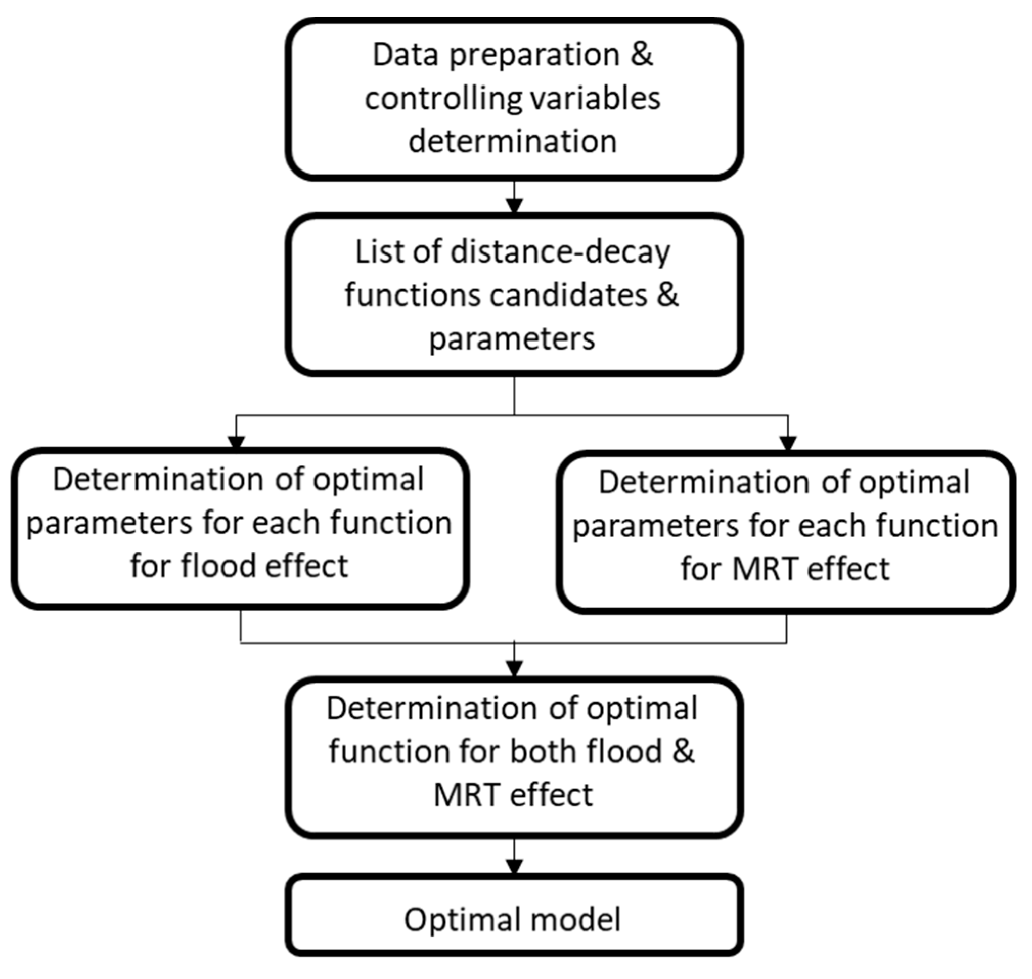
The illustration of conceptual framework of this study is as shown in
Figure 3.
4. Results and Discussion
4.1. Determination of Optimal Parameters
This study uses the method of minimum residual sum of squares to determine the optimal form and parameters for each distance–decay function. For each function type, several candidate parameters are pre-selected to determine the optimal function. For each parameter, a distance effect variable is generated based on the corresponding distance–decay equation, reflecting a decay of the perception of home buyers towards flood risk or MRT accessibility with distance. These distance variables are then added into a regression model with fixed control variables. The distance variable that results in the smallest RSS for the regression model is presumed to be the optimal function to capture homebuyer perception decay patterns. This function and the corresponding parameters are considered as the optimal decay function for a certain distance effect.
We use the determination of the parameters for the inverse of distance for the flood risk as an example to further illustrate the optimization process. The regression results are listed in
Table 3. In this case, two patterns reflecting how the flood effect decays over distance (
y =
x), the inverse of distance (
y = 1⁄
x) and the squared inverse of distance (
y = 1⁄
x^2), are compared. Both distance-to-flood variables are added into a hedonic price regression model with identical variables, including property characteristics (area, age, floor level, building type, number of rooms, the existence of management committee, and parking spaces), and neighborhood characteristics (distance-to-MRT, nearby parks). Note that RSS values obtained for both models with flood variables are less than that identified for the blank model (with no flood variable), showing that the inclusion of distance-to-flood effect helps to explain the difference in sales prices. The result shows that using the inverse of distance to describe the decay of flood effect yields the smallest RSS, which indicates that the optimal equation form for this group is the inverse of distance.
Note that most of the controlling variables included in the model are statistically significant, and the R-squared value is relatively high even for the blank model. Both shows that the model has good explanation power. In addition, the significances are consistent among models, indicating the stability of the model. The meaning of coefficients for each variable is not addressed here because OLS regression for spatial data usually raises the concern for endogeneity and heterogeneity [
6], which might bias the coefficients. The purpose of this study is to determine the optimal distance–decay function that fit home buyers’ perception changes through RSS changes. Theoretically, endogeneity and heterogeneity do not alter the relative explanation power of the model. Thus, OLS regression model still serves well for the purpose of this study.
Following the same procedure, the optimal equation forms for each function type, and for both distance-to flood and MRT accessibility effect are listed in
Table 4. Note that while determining the optimal function type for one of the variables of interest, the function type for the other variable must be holding constant so that the RSS of different models can be directly comparable. For the convex group (inverse of distance and negative exponential), the optimal form for the flood effect and MRT accessibility are identical. For the concave group and the buffer zone, optimal parameters for the flood effect and MRT accessibility vary significantly. The result clearly indicates that the range of impact for MRT accessibility is generally smaller than that for the flood effect. For example, the optimal parameter for describing the decay of flood effect as an ellipse is 2000, which means that the impact of flood risk on housing prices does not fade away until the flood area is 2000 m away. On the other hand, the premium of being close to MRT exits fades quickly after 800 m if the decay curve is described as an ellipse. This result is inconsistent with our expectations. One possible explanation is the degree of uncertainty. The location of flood occurrence is much more uncertain compared with the location of MRT exits. Facing a risk of uncertainty, people tend to err on the side of caution and locate themselves further away. The benefit of access to public transportation is relatively certain. The impact range for public transport found in this study is generally consistent with that identified in other studies [
23,
24].
4.2. Comparison of Distance–Decay Functions
This study aims to further determine the optimal distance–decay function for each distance effect by comparing RSS values of function types. The results for the effect of distance-to-flood and MRT accessibility are listed in
Table 5 and
Table 6, respectively. As shown in
Table 5, the coefficients for all distance variables are significant and negative, indicating that the effect of flood risk on housing prices decays over distance, no matter how the decay pattern is described. However, the result of RSS reduction indicates that concave functions are more suitable when describing the pattern of how flood risk decays over distance. Compared with the blank model (with no distance-to-flood variable), RSS for models with concave distance–decay variables are significantly reduced by more than 10%. For example, by including a variable which describes the distance-to-flood effect as a squared decay curve that vanishes over 2000 m, the unexplained residual is reduced by 10.7%. This is a significant reduction for a model with thirteen controlling variables. As a comparison, describing the distance–decay pattern as a negative exponential curve only improves the RSS by 0.2%. This result clearly indicates that the decay pattern over distance does matter in terms of the explanation power of the model. For the case of flood effect decay over distance in Taipei, using concave functions is clearly more suitable than other function types.
The results in
Table 6 show similar trends. The positive effect of MRT accessibility on housing prices significantly decays over distance, no matter how the decay pattern is described. Similarly, the explanation power for models with concave distance variables are significantly better than those for other function types. In the case of MRT accessibility in Taipei, it is more suitable to describe the premium decay of accessing MRT using a concave function.
5. Conclusions
This study illustrates the pattern of the perception of home buyers decaying over distance. A process based on ordinary least square regression is tested in the case of Taipei to determine the optimal perception decay curve. For both tested distance effects, the flood risk, and the mass rapid transit (MRT) accessibility, the perception decay pattern can be best represented by concave curves, where the effect decays slowly at first and then decreases rapidly after a certain distance. The result for the flood perception is not as expected because the perception change pattern towards natural hazards is usually recognized as either buffer zone or convex curves, in which the effect falls off drastically over a short distance.
In addition, the result further indicates that the impact range varies between flood risk and public transportation accessibility. The impact range for flood risk is generally larger than that for MRT exits. This result implicitly identifies the spillover of risk perception of homebuyers, because the perception impact range of 2 km is much larger than the actual impact range of flood events.
These results have policy and methodological implications. On the policy side, the results support the need for the Government to improve infrastructure and protect against natural hazards. Since the perception impact range of flood risk is larger than expected, the benefit of mitigating flood events is larger than expected in terms of social benefit; this can be quantified as the prevention of loss in residential property values. On the methodological side, the optimization process developed in this study is a useful tool when determining a more accurate distance variable in a model.
There is limitation for this study. The developed method is only tested in a specific area within a short period of time. The policy suggestion based on the results of this study is not necessarily applicable to other cities or contexts. Further studies based on this methodology are required before the proposed optimization process can be fully validated.


