Article

Mixed Land Use Evaluation and Its Impact on Housing Prices in Beijing Based on Multi-Source Big Data

1
School of Land Science and Technology, China University of Geosciences, Beijing 100083, China
2
State Key Laboratory of Remote Sensing Science, Aerospace Information Research Institute, Chinese Academy of Sciences, Beijing 100101, China
*
Author to whom correspondence should be addressed.
Land 2021, 10(10), 1103; https://doi.org/10.3390/land10101103
Submission received: 2 September 2021 / Revised: 12 October 2021 / Accepted: 16 October 2021 / Published: 18 October 2021
(This article belongs to the Section Urban Contexts and Urban-Rural Interactions)

Abstract

:
The tense relationship between the supply and demand of land resources and the past spatial expansion of urban development in Beijing have brought many urban problems. Mixed land use is considered to be able to solve these urban problems as well as promote sustainable urban development. In this context, this study uses multi-source big data such as POI, OpenStreetMap and web crawler data to construct current land-use data of the area within the sixth ring road of Beijing, and then uses the entropy index and type number index to analyze the spatial distribution and aggregation characteristics of the mixed land-use level. Finally, a multi-scale geographically weighted regression is applied to explore the impact of the block and life circle scale mixed land use on housing prices. The results show that: (1) the accuracy of land use data obtained by using multi-source big data is high, and the consistency with the real land use situation is as high as 82.67%. (2) the mixed land use level in the study area is higher in the urban center and lower in the periphery of the city. However, it does not show the spatial distribution characteristics gradually decreasing with the increase of the distance from the urban center but shows that the area from the third to the fifth ring road is the highest. (3) the impact of block scale and life circle scale mixed land use on housing price is different. The type number index has a negative effect on the housing price in block scale mixed land use, while the entropy index has a positive effect on the housing price in life circle scale mixed land use. Based on the existing “bottom-up” individual-dominant development mode, the government of Beijing should issue relevant policies and documents to give “top-down” control and guidance in the future, so as to promote the maximization of the benefits of mixed land use. Furthermore, in the practice of mixed land use in Beijing, land use types should be reduced at the block scale and the area of different land use types should be balanced at the life circle scale.

1. Introduction

Since the beginning of the 20th century, urban development has caused numerous urban problems, such as congestion, serious air pollution, endless urban sprawl, and inappropriate land development with low urban density [1]. Scholars believe that these urban problems are caused by urban functional zoning [2]. Mixed land use emphasizes compatible land use in a parcel, it is an important indicator of land use development mode and diversity [3,4]. It is also an important aspect of modern urban planning concepts such as “New Urbanism”, “Shrinking City” and “Smart Growth”, and is considered as one of the important solutions to alleviate and solve the current urban problems. Although studies indicate that mixed land use will lead to traffic congestion, land occupation, high-density housing, parking difficulty, chaos and noise, stressed infrastructure, and the like [5], more research have confirmed the important role of mixed land use in promoting intensive land use, sustainable urban development, and compact cities [6,7,8]. Moreover, it can also bring about the improvement of cognitive and structural social capital and improve urban vitality [9,10,11]. Mixed land use can alleviate traffic pressure and traffic congestion by reducing cross-regional travel, significantly reducing commuting time and alleviating the separation of work and residence [12,13,14,15,16]. In addition, mixed land use can reduce regional energy consumption and carbon emissions, promote the improvement of residents’ health, and improve the quality of urban living, making the urban environment more livable [17,18,19,20,21,22,23].
As an important way of urban land use, there are some studies about the relationship between mixed land use and housing prices. Although there is a study revealing that mixed land use can reduce housing prices but increase housing rent [24], most studies have confirmed its positive impact on housing prices. These studies believe that proper mixed land use can assist in providing a greater quantity of affordable rental units, increasing investment in properties, and promoting higher property values [25,26,27]. This is because an increase in industrial, commercial, multifamily, and public land use activities in a neighborhood tends to increase the property value of surrounding residential areas [28]. Further, housing prices were found to be higher in the residential areas dominated by residential land and the even distribution of non-residential land [29,30]. Although mixed land use may affect a residential community’s living environment, the resulting accessibility often outweighs any nuisance costs when the quantity, quality, and spatial distribution of non-residential land are carefully integrated into residential neighborhoods [31].
The positive impact of mixed land use on urban development has been confirmed. However, the existing planning management system in China does not define mixed land use nor provide a corresponding management model, making the development of China’s mixed land use highly self-organized and thus a highly valuable research topic [32]. Shenzhen and Shanghai took the lead in issuing relevant policy documents to experiment with mixed land use, while Beijing, as the capital of China and a megacity with a population of more than 20 million, has yet to issue relevant policy documents. On one hand, limited land resources prevent Beijing from continuing its past urban development of spatial expansion; on the other hand, many problems need to be solved urgently in Beijing, such as high housing prices, separation of work and residence, air pollution, and traffic congestion, which indicate that Beijing’s urban development should pay sufficient attention to mixed land use. Therefore, it is necessary to evaluate the current situation of mixed land use in Beijing and study its impact on housing prices.
Although the existing research on mixed land use has involved various fields, they are only used as part of the research, not the main body of the research. The research units in the existing studies are mostly grid units and oversized administrative units with a significantly large area, which cannot reflect the real land use situation. In addition, land use data in these studies mostly comes from government departments, which is not only slow to update but also difficult to obtain. Therefore, the main purpose of this paper is based on multi-source big data, with mixed land use as the main body of the research to explore the spatial distribution characteristics of mixed land use and examine the impact of mixed land use on housing prices at different scales in the study area. The analysis of the spatial distribution characteristics of mixed land use is hoped to attain the current situation of mixed land use in the area within the sixth ring road in Beijing and draw the city’s attention to mixed land use. The examination of the relationship between mixed land use and housing prices is to give specific suggestions for the implementation of mixed land use. The specific research objectives are as follows. (1) Based on multi-source big data, by determining the definition, proportion standard and calculation method of mixed land use, the land use data based on blocks can be formed that can reflect the real land use situation of the city. (2) Based on the obtained land use data, by selecting indicators that can measure mixed land use level, the overall level of mixed land use and its spatial distribution characteristics are analyzed in the study area. (3) Selecting a more robust model to explore the spatial heterogeneity of the impact of mixed land use on housing prices and the spatial scale of this impact. (4) Exploring the difference of the impact of mixed land use on housing prices at different scales, and provide specific implementation suggestions accordingly.
Therefore, in this study, big data such as POI data, OpenStreetMap road data, and housing price data were used to construct land use data in the area within the sixth ring road in Beijing. Within this study area, the mixed land use degree by entropy index and type number index is measured, and its spatial distribution and spatial aggregation are explored. Finally, a multi-scale weighted geographically regression model is used to explore the spatial heterogeneity and scale effect of the impact of mixed land use on housing prices. Compared with the existing studies, this study mainly has the following contributions. (1) Using multi-source big data as the research data not only reduces the difficulty of data acquisition but also improves the reproducibility of research methods. (2) A method and procedure for using big data to obtain land use data is proposed. (3) Taking mixed land use as the research subject and conducting an empirical study to explore its spatial distribution characteristics and its relationship with housing prices in the study area. (4) The use of a newer multi-scale geographically weighted regression model enriches its empirical research and confirms its superiority compared with traditional models. (5) The impact of mixed land use on housing prices at different scales is explored, and the advantages of different scales can be complemented and specific suggestions on mixed land use at different scales can be given.

2. Materials and Methods
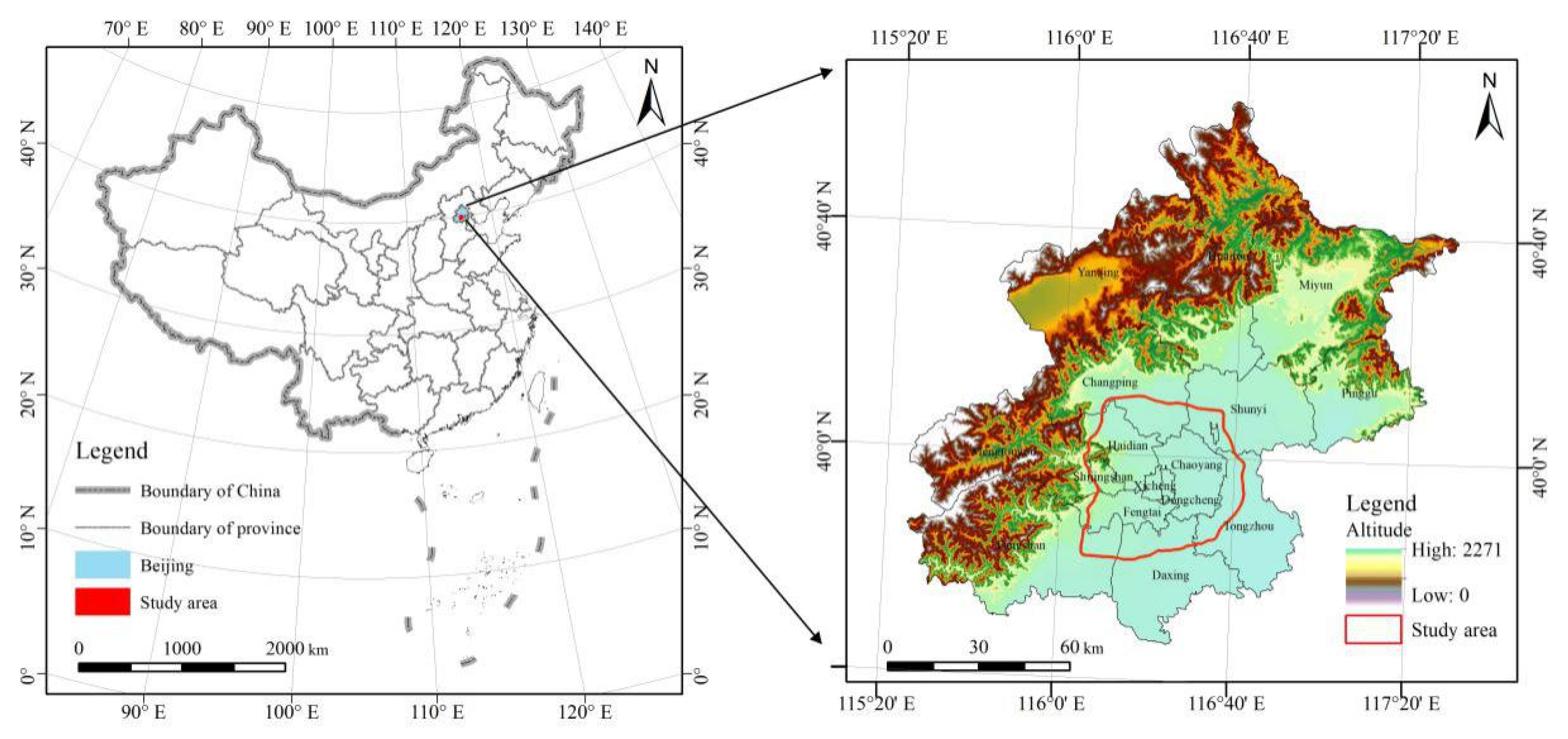
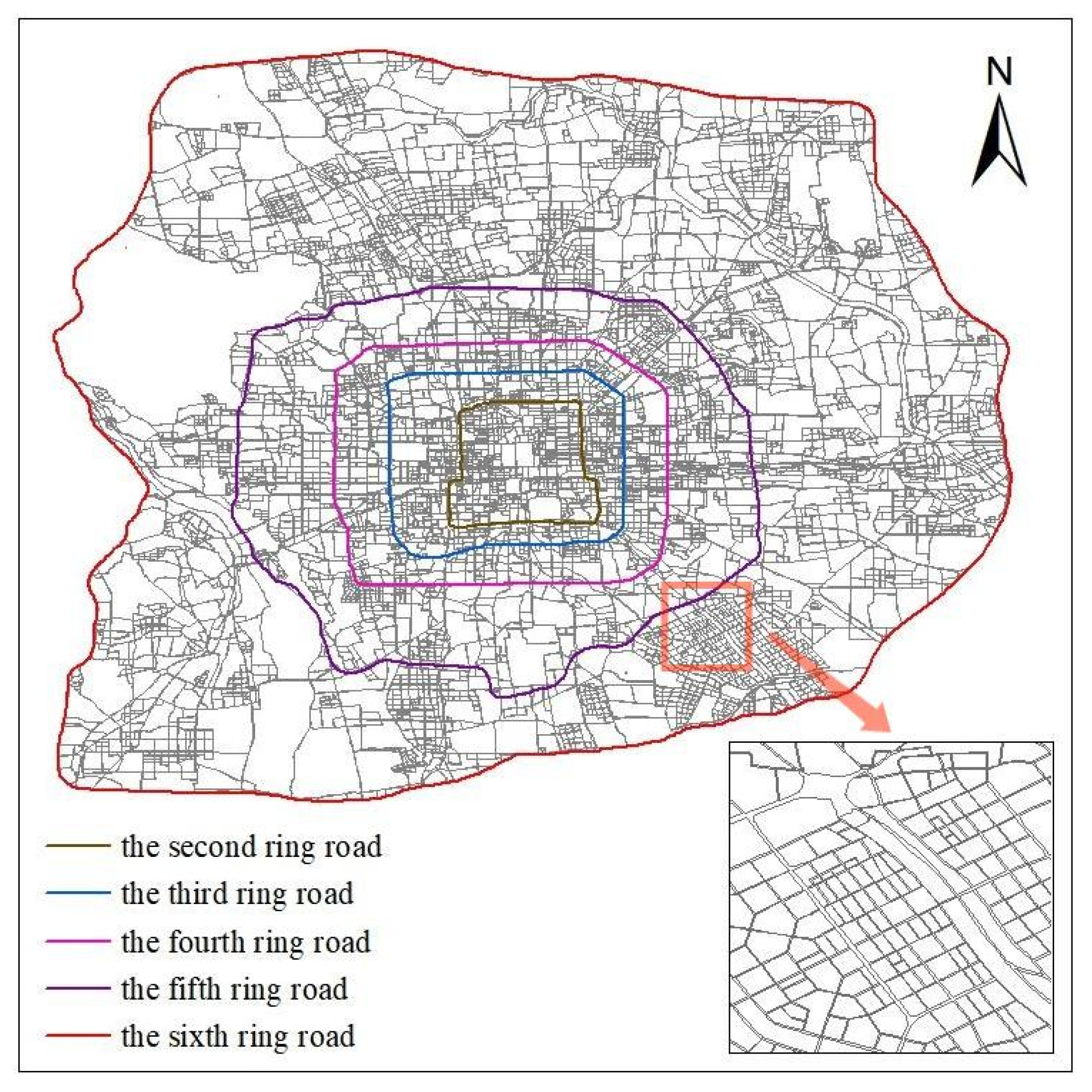
2.1. Study Area

Beijing, the capital city of China, is the political, cultural, international exchange, and scientific and technological innovation center of the country. It is a national central city and a megacity. With a land area of 16,410.54 km2 and a permanent resident population of 21.536 million in 2019, the development of the city is facing tremendous pressure on land resources and population. Furthermore, Beijing has the most serious separation of work and residence in China, with an average one-way commuting time and distance of 47 min and 11.1 km, respectively. Therefore, the status of mixed land use in Beijing is of great research value. Beijing is located in the northern part of the North China Plain and is surrounded by mountains on three sides. It is a typical city with a single-center structure and the main functions, population, and facilities are concentrated in the area within the sixth ring road. Therefore, this article studies an area within the sixth ring road in Beijing. The scope of the study area is shown in Figure 1.

2.2. Data Source and Processing

2.2.1. Data Source

This study uses three data sources: Gaode Map POI, OpenStreetMap road data, and housing price data. POI (point of interest) data were obtained on the Gaode Map Open Platform (map.gaode.com, accessed data: 1 September 2021) through an application program interface (API) in 12 October 2017. The data include details such as the classification, name, address, longitude, and latitude of various facilities. The benefit of POI data is that they can represent a much finer-grained picture of land use at the building level [33]. Road data on Beijing was obtained from the official website of OpenStreetMap (www.openstreetmap.org, accessed date: 1 September 2021) in 8 December 2017. The advantage of using this data as the research unit boundary is that it can reflect the real land use situation based on the urban form and structure. Furthermore, in 17 December 2017, details such as housing prices, longitude and latitude, plot ratios, greening rates, property management fees, and building ages of residential communities in Beijing were obtained from FANG.com (accessed date: 1 September 2021) using a web-crawling Python program. To avoid biased results that newly built apartments may cause, we only collected the information of second-hand apartments. After cleaning and processing the data, a total of 3725 residential communities in the study area was determined.

2.2.2. Construction of Land Use Data

The construction of land use data can be divided into three steps.
The first step is to determine the definition and proportion standard of mixed land use in this study. Based on the definition of mixed land use in the “Shenzhen Urban Planning Standards and Guidelines (2019)” and “Shanghai Regulatory Detailed Planning (2016)”, this study defines mixed land use as two or more land use types in the same block. The block with one land use type occupying more than 70% area in the block is defined as a single-function block, and the land use type of the block is the land use type with an area accounting for more than 70%. The blocks in which the area proportion of each land use type in the block is less than 70% are defined as mixed-function blocks. Since the functions with an area ratio of less than 10% are generally considered as ancillary facilities supporting the main functions, the functions with an area ratio of less than 10% in the mixed-function blocks are ignored, and the land use type of mixed-function blocks are only the land use types with an area ratio of 10–70%.
The second step is the selection of land use types and the calculation of area proportions. This study selected six urban land use types, namely, industrial land, public management and service facilities land, transportation facilities land, residential land, green space and square land, and commercial service land. A total of 29 POI types corresponding to six land use types (Table 1) were selected to realize the identification of block functions. By selecting 30 samples for each type of POI, the average area is obtained on the map and the area weight is determined according to the average area. The area weight of each type of POI is shown in Table 1. The area of a POI can be estimated by the quantity and area weight, and then the area and proportion of each land use type can be calculated accordingly.
The third step is block extraction, function recognition, and accuracy verification. The road data obtained on the OpenStreetMap official website are line files. Firstly, unimportant and unclosed short roads are deleted, and the unclosed roads are extended to make them closed according to the electronic map. Then, the buffers of different grades of roads are established, respectively, and combined to obtain the surface data of all roads in the city. Finally, road surface data is used to erase the surface data of the study area, and the erased data is split to make each block a separate plot. Using this method in the study area, a total of 6488 blocks were obtained (Figure 2).
The POI data is overlayed with the block data and the number of each POI type is calculated. Then, the area proportion of different land use types and land use type of each block are calculated and identified. The constructed land use data within the sixth ring road of Beijing is shown in Figure 3. In order to judge the accuracy of the data, this study randomly selected 100 block units. The recognition results with the real land use conditions are compared, and the conformity degree is judged by scoring. The scores were divided into four levels, where 0, 1, 2, 3 represent complete inconsistency, relatively inconsistency, relatively consistency, and complete consistency, respectively. The ratio between the total score and full score of the sample marks is the value of the conformity degree. In this study, the conformity degree between the identification results and the real situation is 82.67%, indicating that the accuracy of land use type identification by this method is high and the data can be used for further research and analysis.

2.3. Methods

2.3.1. Indicators of Mixed Land Use

In general, the measurement of mixed land use is currently based on two dimensions: distance and quantity [34]. Some commonly used indicators are percentage and proportion, as well as balance, entropy, Herfindahl–Hirschman, Atkinson, clustering, dissimilarity, and Gini indexes [35]. This study uses entropy index and type number index to indicate the mixed land use degree in the block. The entropy index is used to reflect the equilibrium degree of the area or quantity of various land use types in the block, while the type number index is used to reflect the richness of land use types in the block.
(1)
Entropy Index
The entropy index is usually used to measure the equal occurrence degree of different functions and diversity in a region [36,37]. This index can therefore be used to measure the equilibrium degree of the area or quantity of different land use types in the block. The value ranges from 0 to 1, where 0 indicates homogeneous land use and the lowest equilibrium degree, and 1 implies the even distribution of the number or area of all land use types in the block and the highest equilibrium degree. The greater the value of this index, the higher the mixed land use degree. In this paper, the entropy index is represented by ENTROPY, and the calculation method is as follows:
E N T R O P Y = [ j = 1 k P j ln ( P j ) ] / ln ( k )
where Pj is the proportion of land use type j in the parcel, k ≥ 2 is the number of land use type j and ENTROPY is the entropy index.
(2)
Type number index
The type number refers to the number of land use types contained in a block. In this paper, this index is represented by NUMBERS. The value is an integer greater than or equal to 0. The larger the value, the richer the land use types contained in the block and the higher the degree of mixed land use.

2.3.2. Spatial Autocorrelation

In this paper, the global spatial autocorrelation is used to judge whether the entropy index and type number index are clustered in space, and the local spatial autocorrelation is used to identify their clustering relationship and spatial location of agglomeration. The expressions of global spatial autocorrelation index and local spatial autocorrelation are as follows [38]:
(1)
Global spatial autocorrelation index
I = n i = 1 n j = 1 n W i j ( y i y ¯ ) ( y j y ¯ ) i = 1 n j = 1 n W i j j = 1 n ( y i y ¯ ) 2
(2)
Local spatial autocorrelation index
I i = n ( y i y ¯ ) j = 1 n W i j ( y j y ¯ ) i = 1 n ( y i y ¯ ) 2
In Formulas (2) and (3), I is the global autocorrelation index, Ii is the local autocorrelation index, n is the total number of block units, yi and yj is the entropy index or type number index of the block unit i and the block unit j, respectively, ӯ is the mean value of the entropy index or type number index, and Wij is the spatial weight matrix. In the global spatial autocorrelation, the value of I is between [–1, 1]; I > 0 indicates a positive correlation and agglomeration distribution in space, I = 0 indicates a random distribution and I < 0 indicates a negative correlation and discrete distribution in space. When, |Z| > 1.96 the spatial autocorrelation of variables is significant. In the local spatial autocorrelation, the clustering relationship mainly includes high-high agglomeration (HH), high-low agglomeration (HL), low-high agglomeration (LH), low-low agglomeration (LL) and no obvious agglomeration.

2.3.3. Multi-Scale Geographically Weighted Regression Model

In order to reflect the spatial scale difference of the relationship between independent variables and dependent variables, Fotheringham proposed a multi-scale geographically weighted regression model (MGWR) in 2017 [39]. Yu et al. supplemented and improved the statistical inference of MGWR in 2019 so that this method can be widely used in empirical research [40]. Compared with the traditional GWR model, the MGWR model selects different bandwidths according to different variables to produce a more realistic and useful spatial process model. At the same time, it can further compare the influence scale of each variable. The bandwidth reflects the spatial heterogeneity of the relationship between independent variables and dependent variables [41]. The calculation formula of the MGWR model is as follows:
y i = j = 1 k β b w j ( u i , v i ) x i j + ε i
where (ui, vi) is the coordinate of the sample point, k is the number of independent variables, bwj represents the bandwidth used by the regression coefficient of the j-th variable, βbwj represents the regression coefficient of the j-th independent variable fitted with a specific bandwidth, and εi is a random error term.
According to the hedonic hypothesis, goods are valued for their utility-bearing attributes or characteristics. Housing characteristics are typically classified into three categories: structure, location, and neighborhood [42]. As such, this study selected independent variables based on these three housing characteristics and added independent variables that can reflect the mixed land use degree to study the impact of mixed land use on housing prices. This study used two models to study the impact of mixed land use on housing prices. Model 1 studies the impact of the mixed land use in the block where the residential community is located on the housing price; as the size and shape of blocks are different, the size of the research unit is different. Model 2 studies the impact of the mixed land use in the life circle where the residential community is located on the housing price; each research unit has the same size and shape (circular area), with the residential community forming the center and has a 1000 m radius. The block and life circle where the residential community is located are shown in Figure 4. In this study, we expected a numeric confirmation to the hypothesis that the mixed land use has a positive impact on housing prices.
The calculation formulas of Model 1 and Model 2 are as follows:
Model 1:
y i = β b w m 1 ( u i , v i ) x i m 1 + β b w s ( u i , v i ) x i s + β b w l ( u i , v i ) x i l + β b w n ( u i , v i ) x i n + ε i
Model 2:
y i = β b w m 2 ( u i , v i ) x i m 2 + β b w s ( u i , v i ) x i s + β b w l ( u i , v i ) x i l + β b w n ( u i , v i ) x i n + ε i
In Formulas (5) and (6), m1 is the mixed land use degree in the block where the residential community is located, m2 is the mixed land use degree in the life circle where the residential community is located, s is the structural characteristics of the residential community, l is the location characteristics of the residential community and n is the neighborhood characteristics of the residential community.
The advantage of Model 1 is that it can reflect the real land use status and urban form, but the disadvantage is that the size of the research unit is inconsistent. In addition, land use has externalities. That is, the land use in the residential area and the land use in the surrounding area will affect each other. The influence range is roughly 15 min over a walking distance of about 1000 m, which is the range of the life circle. Therefore, Model 2 can not only consider its interaction with the surrounding land use but also makes the size of the research unit consistent. The disadvantage of Model 2, however, is that it cannot reflect the real land use situation. The two models can not only complement each other’s advantages, but also reflect the difference of the impact of mixed land use on housing prices at different scales, and can put forward suggestions on mixed land use accordingly. In both models, the independent variables are the same except for the entropy index and type number index. Other independent variables mainly include BUILDING AGE, FEE, GREENING RATIO and PLOT RATIO that reflect the structural characteristics of the residential community, CITY CENTRE, SUBWAY and SHOPPING MALL that reflect the location characteristics of the residential community, and PARK, HOSPITAL, SCHOOL, and BUS that reflects the neighborhood characteristics of the residential community. The specific variable descriptions are provided in Table 2.

3. Results

3.1. Mixed Land Use Evaluation

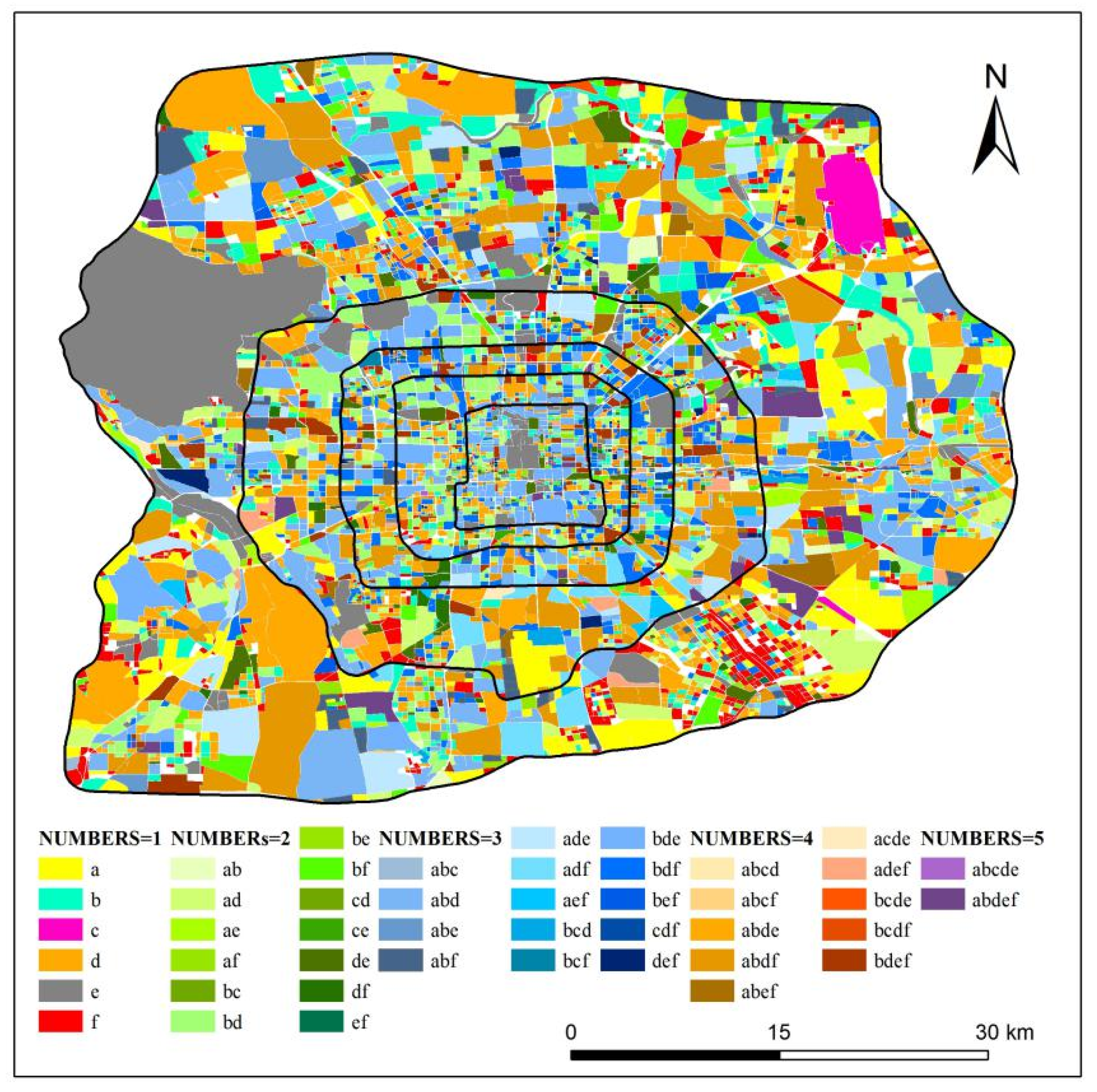
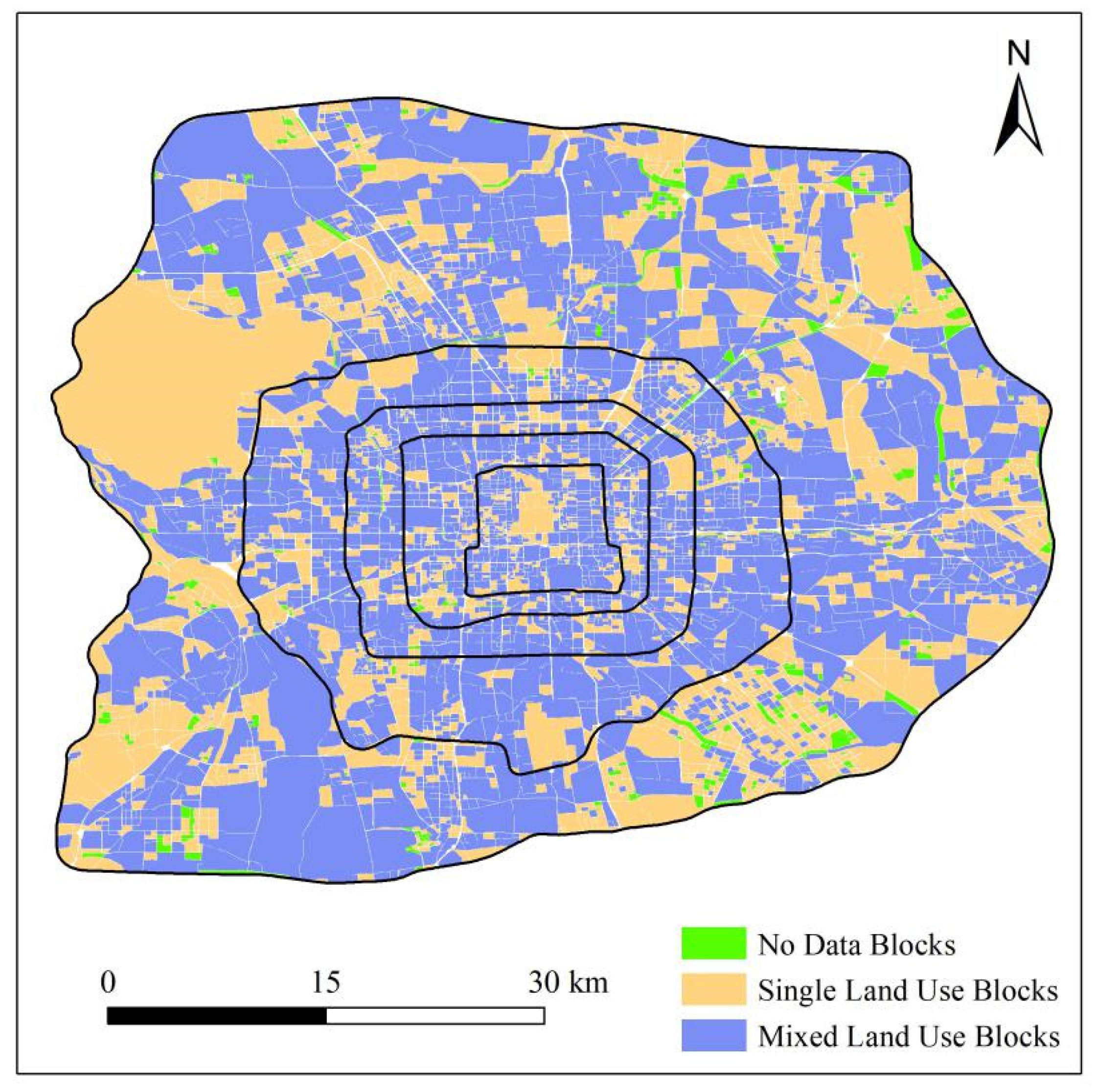
3.1.1. Spatial Distribution of Mixed-Function Blocks

Among the 6488 blocks in the area of Beijing’s sixth ring road, the number of no data blocks, single-function blocks, and mixed-function blocks accounted for 8.80%, 44.57%, and 46.63%, respectively. In the study area, the proportion of mixed-function blocks is the highest and the overall level of mixed land use is relatively high. As can be seen from Figure 5, mixed land use widely exists within the sixth ring road in Beijing, especially within the fifth ring road, while single-function blocks are mainly distributed in the urban periphery from the fifth to the sixth ring road. To some extent, this reflects that the land use in the central area of the city is relatively intensive, while land use in the peripheral areas of the city is relatively extensive.
From the fifth to the sixth ring road of the city, the mixed land use level is low, and there are a large number of single-function blocks. This is mainly due to the fact that the land use in this area is mostly single functional groups and characterized by large land occupation. This includes large-scale high-tech industrial parks, university towns where new university campuses are concentrated, mountainous areas in the west, and large residential areas due to exorbitant housing prices in the urban center. The exorbitant housing prices in the city center and functional zoning are also important reasons why Beijing may become the city with the most serious phenomenon of job-housing imbalance in China.

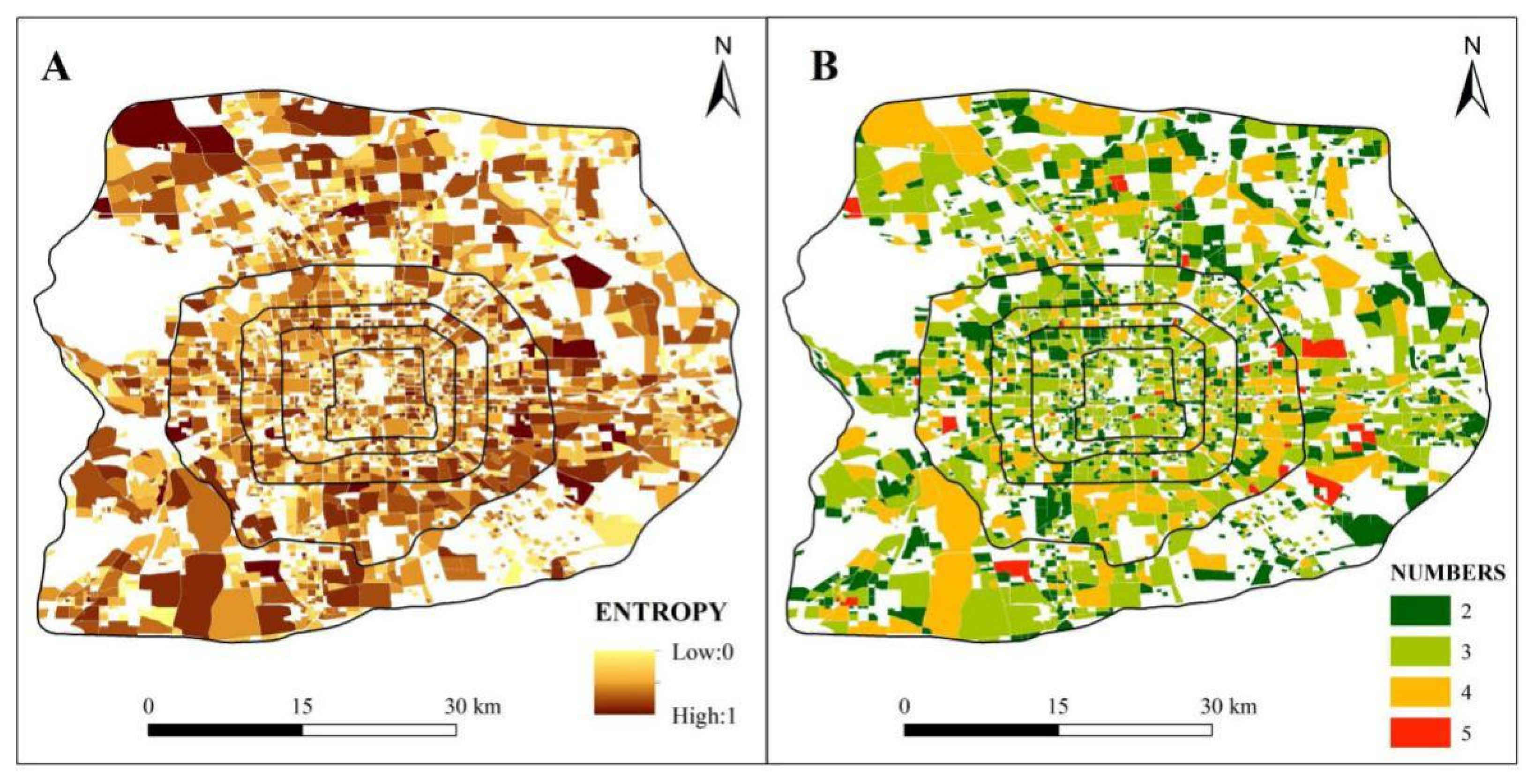
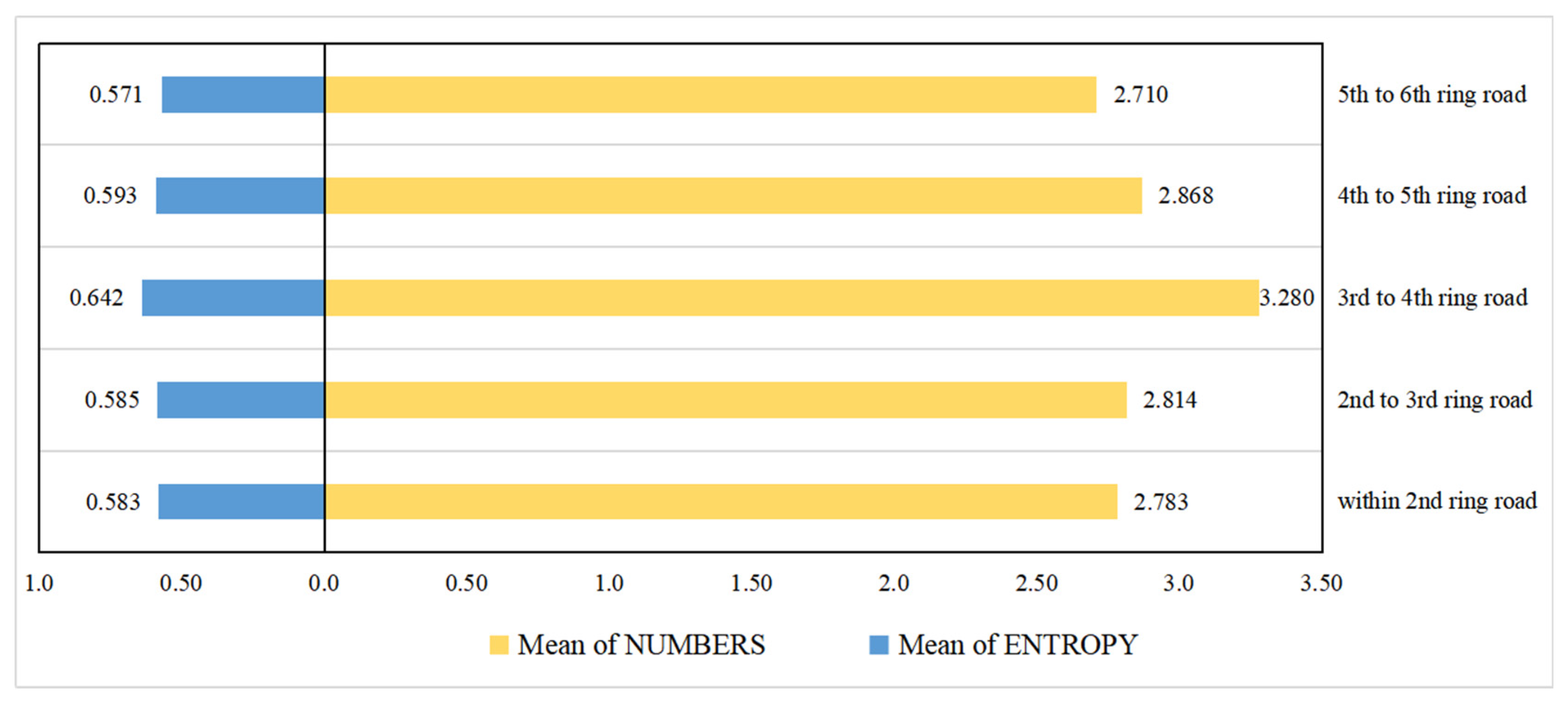
3.1.2. Spatial Distribution of Mixed Land Use Indicators

The spatial distribution of the entropy index and the type number index in the study area is shown in Figure 6 and their corresponding mean values in each loop are shown in Figure 7. The mean value of the entropy index is the highest in the region from the third to the fourth ring road, high in the region from the fourth to the fifth ring road, medium in the region from the second to the third ring road, low in the region within the second ring road, and lowest in the region from the fifth to the sixth ring road. The mean values are 0.6418, 0.5926, 0.5851, 0.5825, and 0.5713, respectively. The distribution trend of the mean value of type number index is the same as that of entropy index; that is, highest in the region from the third to the fourth ring road, high in the region from the fourth to the fifth ring road, medium in the region from the second to the third ring road, low in the region within the second ring road, and the lowest in the region from the fifth to the sixth ring road, with mean values of 3.2797, 2.8684, 2.8144, 2.7834, and 2.7099, respectively. In this study, the average value of entropy index and type number index in the region from the third to the fifth ring road is the highest, followed by the urban central area within the third ring road. The average value of entropy index and type number index in the region from the fifth to the sixth ring road is the lowest.
Existing studies show that the level of mixed land use in urban central areas is generally higher than that in urban peripheral areas [43]. The spatial distribution of mixed land use level in Beijing is different from that in other cities, mainly because due to being a special city—not only is it the national capital, but it is also the ancient capital, which undertakes important political, cultural, national communication and scientific and technological innovation functions. Therefore, various urban planning and land use planning restricts land use within the city. The area within the second ring road is the old city, which not only retains the ancient city-style such as Hutong but also has many historical relics. In addition, it is the gathering place of many central organs of the party, government, and military. Therefore, the urban planning of Beijing is set as an ancient capital style area and a capital function area where land use and construction are highly restricted. Due to the concentrated distribution of hutongs, historical sites, and government agencies, the mixed land use degree in this area is not high. The research of Long et al. [44] shows that the mixed land use level in Beijing presents the spatial distribution characteristics gradually decreasing with the increase of the distance from the city center. However, the results of this study show that the mixed land use level in the area from the third to the fifth ring road is the highest in Beijing. The possible reason for this difference is that previous studies are based on grid units, which, compared to block units, cannot reflect the real urban land use situation.
Generally, the commercial and financial industries in the city will gather in the city center with the highest land price. However, due to high restrictions and controls on land use activities within the second ring road, commercial and financial industries of the city gather in the third ring road area, effectively undertaking the original functions of the city center. The concentration of a large number of commercial and financial industries in this area leads to a significant number of single-function blocks in the area from the second to the third ring road, causing the value of the entropy index and type number index to be low.
Land use in the area from the third to the fifth ring road is not highly restricted (unlike the area within the second ring road), nor is it clustered with a large number of business and financial centers. This makes the combination of land use types in the area relatively free and diversified, resulting in a high mean value of entropy index and type number index, that is, a high degree of mixed land use. The lowest mean value of entropy index and type number index in the area from the fifth to the sixth ring road is in the periphery of the city where economic development and land prices are lower. This has resulted in a concentration of a large number of single-function blocks, leading to the lowest degree of mixed land use.

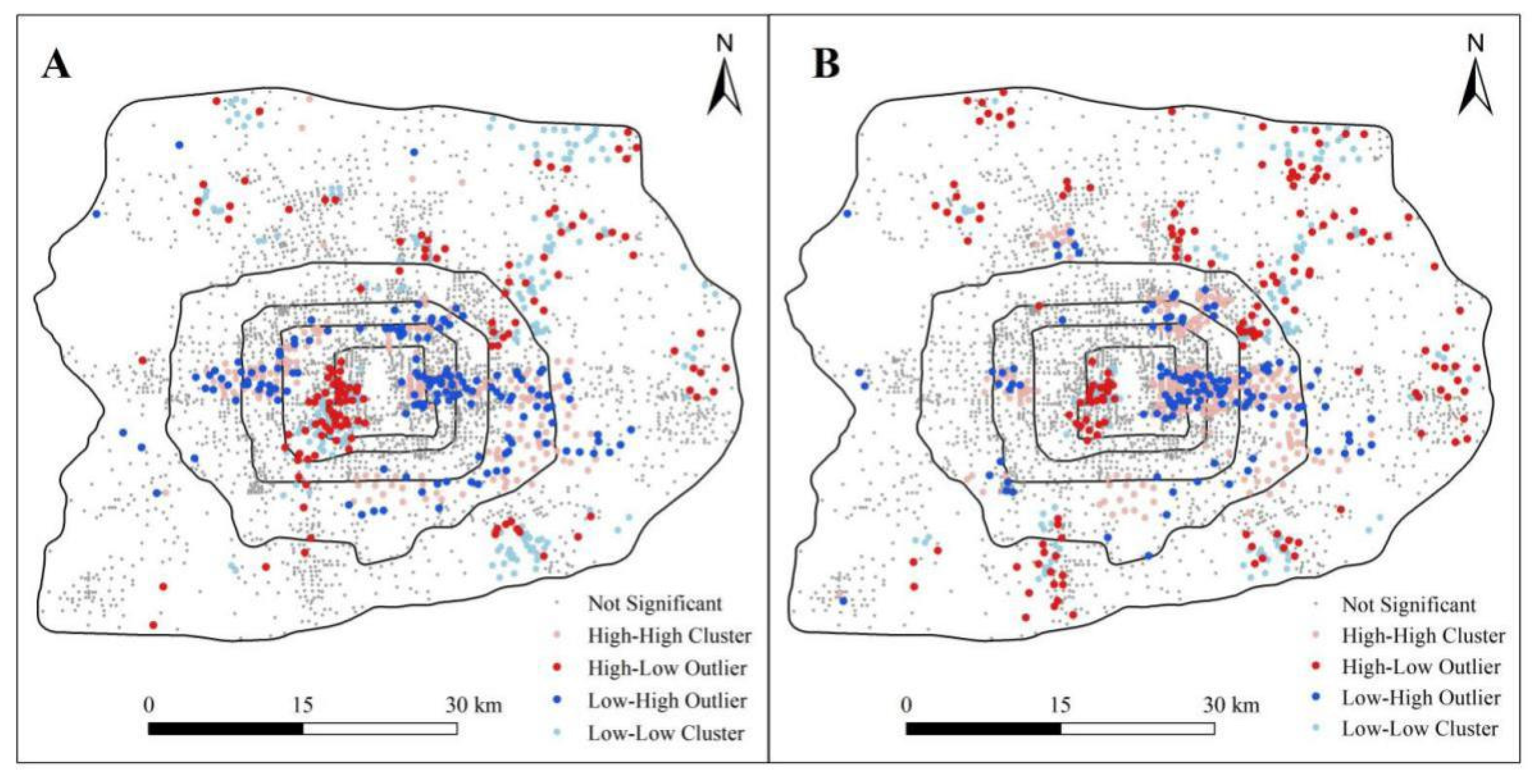
3.1.3. Spatial Agglomeration of Mixed Land Use Indicators

From the results of global spatial autocorrelation, the Moran’s I value of the entropy index is 0.0204, the Z value is 6.05 and the p-value is 0.00; Moran’s I value of the type number is 0.0217, the Z value is 6.43, and the p-value is 0.00. There is a 0% probability that the data distribution is randomly distributed, the probability of aggregated distribution is greater than the probability of random distribution, and the null hypothesis can be significantly rejected. The results show that the spatial distribution of the entropy index and type number index of mixed land use has certain aggregation characteristics and a positive spatial correlation pattern.
Local spatial autocorrelation is used to explore the spatial agglomeration relationship and location of the entropy index and type number index. As shown in Figure 8, both indexes show local spatial aggregation characteristics. High-high agglomeration is mainly distributed in the inner area of the city, while low-low agglomeration is mainly distributed in the outer area of the city. That is, high values of the entropy index and type number index are mainly concentrated in the central area of the city, while the low values are mainly concentrated in the peripheral areas of the city.
Low-high agglomeration is also mainly distributed in urban central areas, indicating that the city center is an area where high values of entropy index and type number are mainly distributed and surround the scattered low values. The results show that the urban central area is the agglomeration area with high values of entropy and type number index, with only a few low values distributed in the area.
High-low agglomeration is mainly distributed in the western area within the second ring road and the urban periphery from the fifth to the sixth ring road. Since the Financial Street in the western region within the second ring road is a national financial management center, the headquarters of national banks and non-bank financial institutions are concentrated there. The agglomeration of financial functions makes the mixed land use degree of the agglomeration area generally low. However, since the agglomeration area is located in the central area of the city, the high value will be scattered in this area. Therefore, high-low agglomeration is formed in the west of the area within the second ring road. High-low agglomerations are distributed in the area from the fifth to sixth ring roads mainly because the overall level of mixed land use in the area being low and a large number of single functional groups. In each group, regional centers will be formed where the mixed land use level is higher than that of other regions in the group. As such, high-low agglomerations with high values surrounded by low values are formed in the area from the fifth to the sixth ring road.

3.2. Impact of Mixed Land Use on Housing Price

Before the regression modeling of housing prices and influencing factors, it is necessary to determine whether there is obvious multicollinearity among influencing factors. The variance inflation factor (VIF) of all influencing factors in Model 1 and Model 2 is less than 4, indicating that no obvious multicollinearity exists between the influencing factors in both models. Therefore, OLS (ordinary least squares), GWR (geographically weighted regression), and MGWR were used for modeling and analysis of housing prices and influencing factors. The model diagnostic information of the three models is shown in Table 3. From the perspective of the adjusted R2, the adjusted R2 value of the multi-scale geographically weighted regression results of Model 1 and Model 2 are the highest, with values of 0.852 and 0.849 that explain 85.2% and 84.9% of the change level of housing price, respectively. In addition, the Akaike Information Criterion (AICc) value and residual sum of squares (RSS) of the MGWR model are also the smallest compared with the OLS model and the GWR model, indicating that the fit of the MGWR model is the best.

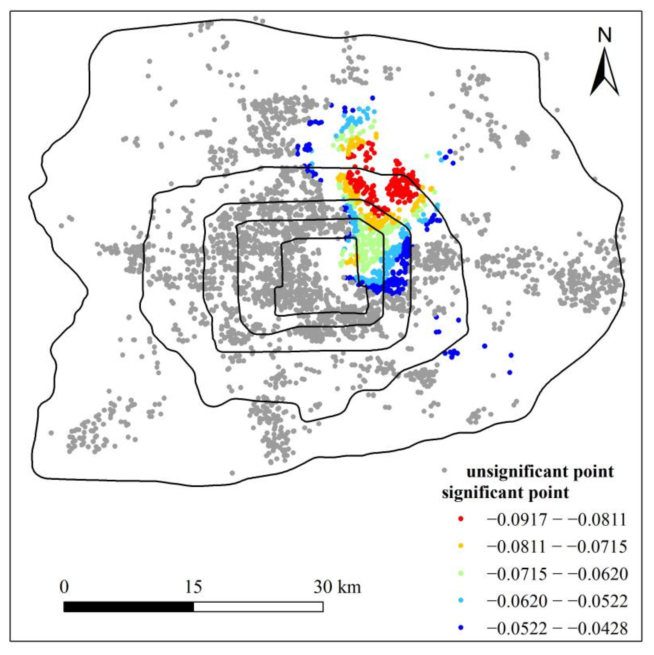
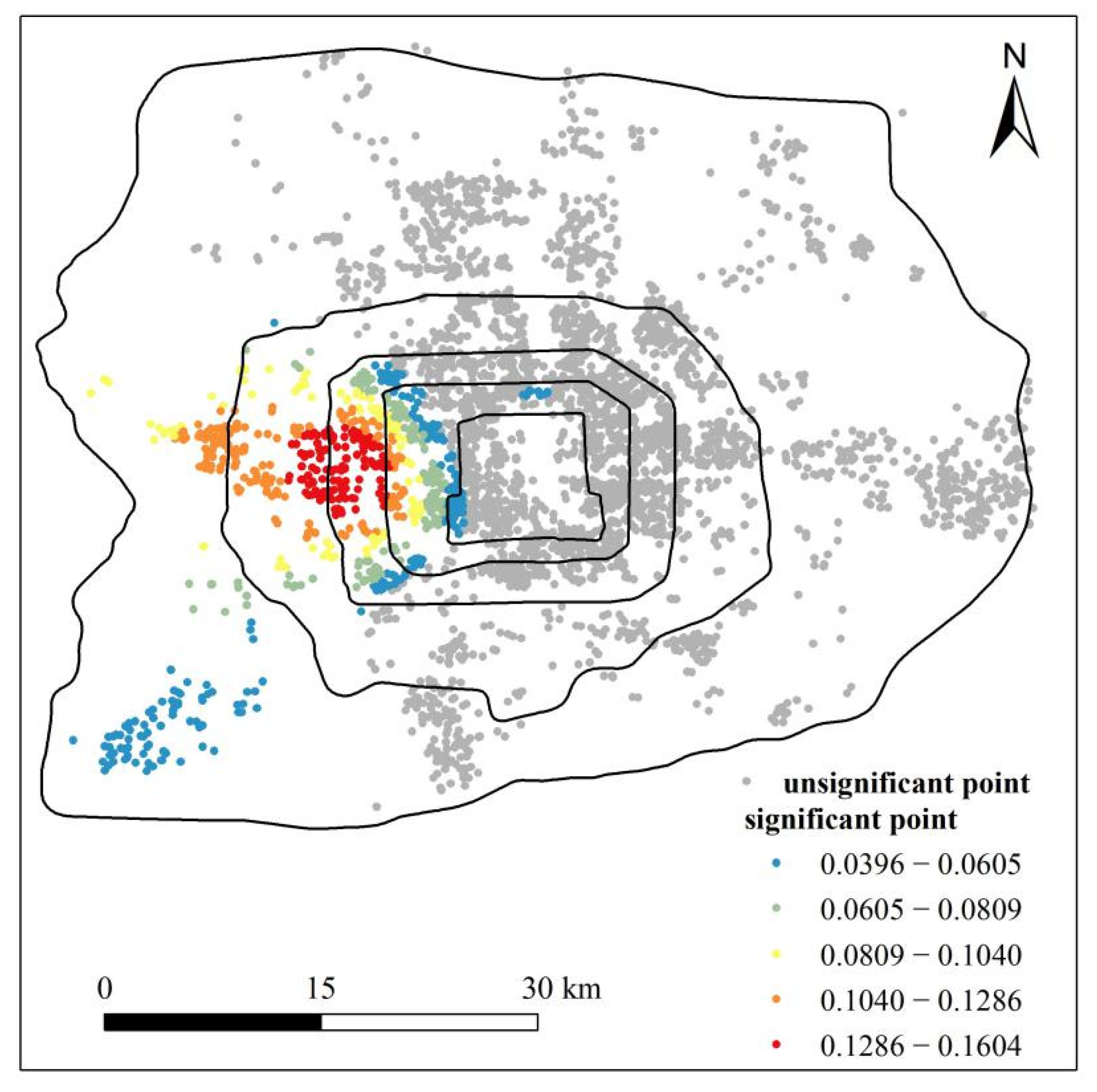
3.2.1. Impact of Mixed Land Use on Housing Price at Block Scale

As shown in Table 4, the number of samples whose p-value of the ENTROPY1 is less than 5% in Model 1 accounts for 0% of the total samples, indicating that the ENTROPY1 has no significant impact on housing prices in the whole study area. Furthermore, 23.16% of the samples in the study area show that NUMBER1 has a significant impact on housing prices. The influence coefficient of the NUMBER1 ranges from −0.092 to 0.027, with an average value of −0.029. The bandwidth of this variable is 776, accounting for 20.85% of the total sample, indicative that there is large spatial heterogeneity in the impact of the type number index on housing prices. From the perspective of the absolute value of the influence coefficient, the influence coefficient of the NUMBER1 is smaller than the influence coefficient of CITY CENTRE, FEE, BUILDING AGE, PLOT RATIO, SUBWAY, GREENING RATE, HOSPITAL, and SHOPPING MALL. This shows that although the type number index of mixed land use in the block scale has a certain impact on housing prices, its influence intensity is not as strong as that of structural characteristics and location characteristics of a residential community.
As shown in Figure 9, by visualizing the influence coefficient of NUMBER1, sample points where NUMBER1 has a significant impact on housing prices are mainly distributed in the northeast of the study area. Moreover, the influence coefficient is negative, ranging from −0.0917 to −0.0428, indicating that the higher the type number of mixed land use within the block scale in this region is, the lower the housing price. This is because a greater number of land use types in a block where the residential community is located will not only increase the flow of people in the area but will also increase the duration of the high-level flow of people. Therefore, it may bring more noise and affect the rest of the residents living in the block. The northeastern part of the study area is an agglomeration area where rich people live, in which there are more high-quality houses and villas. However, since the rich generally prefer to live in houses with beautiful and quiet environments, the type number of mixed land use in this area will have a negative impact on housing prices.

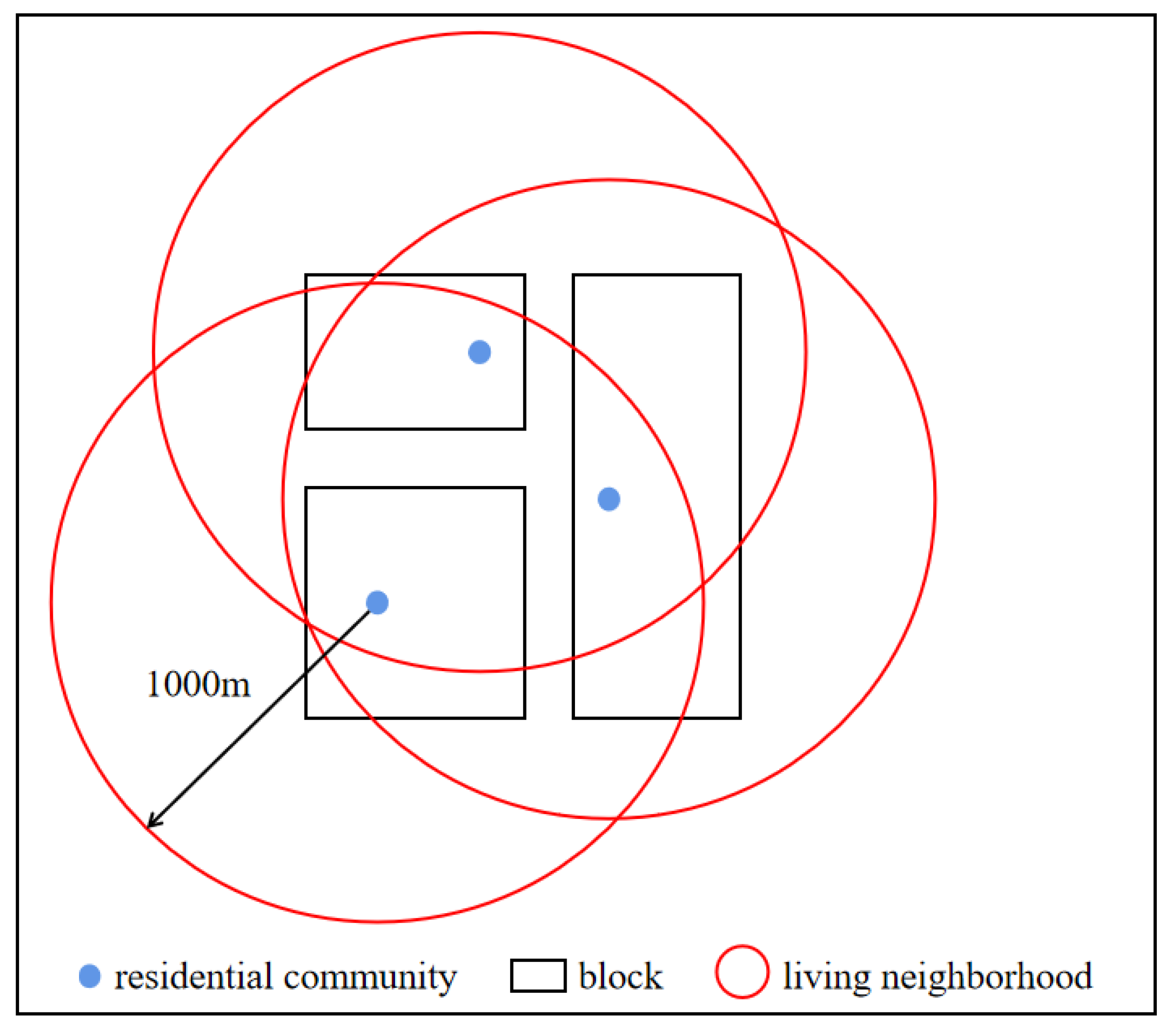
3.2.2. Impact of Mixed Land Use on Housing Price at Life Circle Scale

As shown in Table 5, 20.68% of the samples in Model 2 show that ENTROPY2 has a significant impact on the housing price. The influence coefficient of ENTROPY2 ranges from −0.017 to 0.160 and has an average value of 0.033. The bandwidth of the entropy index is 880, accounting for 23.67% of the total number of samples, indicative that there is large spatial heterogeneity in the impact of the entropy index on the housing price. However, NUMBER2 has no significant influence on the housing price in the whole study area in Model 2. From the perspective of the absolute value of the influence coefficient, the influence coefficient of ENTROPY2 is smaller than the influence coefficient of the CITY CENTRE, FEE, BUILDING AGE, SUBWAY, PLOT RATIO, HOSPITAL and GREENING RATIO. This shows that although the entropy index of mixed land use in the life circle scale has a certain impact on housing prices, its influence intensity is not as strong as that of structural characteristics and location characteristics of a residential community.
As shown in Figure 10, by visualizing the influence coefficient of ENTROPY2, sample points where the ENTROPY2 have a significant impact on housing prices are mainly distributed in the west of the study area. Moreover, the influence coefficients are all positive, ranging from 0.0396 to 0.1604, indicating that the higher the entropy index of mixed land use within the life circle scale in this region is, the higher the housing price. Since the equilibrium degree among various land use types in this region is lower than that of other regions in the study area, the housing price in this region may be more sensitive to the change of the equilibrium degree among various land use types. This makes the entropy index in the western region of the study area have a significant and positive influence on the housing price. To some extent, this shows the importance of a balanced layout among various land use types within the life circle scale, that is, within the 1000 m radius of the residential community.
The results indicated that the land use types should be as rich as possible and that the balance degree of different types is not important in the mixed land use at the block scale. Furthermore, the number of land use types is not important and the balance degree among various land use types is more important in the mixed land use at the life circle scale. Therefore, in the process of real estate development or site selection, there should be as few land use types as possible in the block where the residential community is located to create a good living environment for residents. In the living circle of the residential community, various land use types and various supporting facilities should be evenly arranged to meet the various needs of residents in the residential area and facilitate their life.
The results of Model 1 and Model 2 show that mixed land use does have an impact on housing prices, but not both the entropy index and the type number index have a positive impact on housing price, which is slightly different from our research expectation. To some extent, this study indicates that the impact of mixed land use on housing prices depends on the research scale and the measurement of mixed land use. For mixed land use at the block scale, the entropy index of mixed land use has no effect on housing prices, while the type number index has an effect in the northeast of the study area and its influence coefficient is negative, ranging from −0.0917 to −0.0428. For mixed land use at the life circle scale, the type number index has no impact on housing prices, while the entropy index has an impact in the west of the study area and its influence coefficient is positive, ranging from 0.0396 to 0.1604. The results of this study are different from those of the existing studies, mainly because they only considered the entropy index and did not consider the type numbers in the measurement of mixed land use. Moreover, the research units of the existing studies are larger than those of this study and cannot reflect the real land use situation.

4. Discussion

The results show that the overall level of mixed land use within the sixth ring road in Beijing is high, but this mixed land use is disordered, unorganized and spontaneously based on “bottom-up” individual-dominant development. Beijing has not issued relevant documents to guide the implementation of mixed land use and the existing planning work is still carried out based on functional zoning. Kong et al. believe that “top-down” centrally controlled development may lead to functional zoning, while “bottom-up” individual-dominant development will lead to disorderly and chaotic land use. Only the “bottom-up” collective-dominant development can help to achieve effective mixed land use [45]. Therefore, Beijing should issue relevant policy documents to exercise “top-down” control on the basis of “bottom-up” individual-dominant development, so as to promote the exertion and maximization of the benefits of mixed land use. In addition to issuing relevant documents to control and provide guidance, in the future, government departments and policymakers should also give more attention and policy support for mixed land use, promote the implementation and application of mixed land use, and combine the existing functional zoning with mixed land use to improve the mixed land use level within each functional group. It can not only exert an agglomeration effect but also reduce long-distance transportation in the city and promote the healthy and sustainable urban development of Beijing. In addition, because the mixed land use at different scales will produce different benefits, it is necessary to guide the mixed land use at different scales so as to promote this way of land use and produce higher benefits.
The traditional land parcel recognition method has many drawbacks, such as manual interpretation of remote sensing images and field investigation requiring a lot of labor and time, expensive, and the accuracy of data depends on the experience of data processing personnel. In addition, the data generated by traditional methods are not suitable for regular updating and comparison and it is also difficult to identify the land use types in high-density urban areas [46]. In contrast, using OpenStreetMap data for land parcel identification has many advantages. Firstly, since the OpenStreetMap data is open data, the high availability of data acquisition makes this land parcel identification method easier to replicate and the data can be continuously updated through crowdsourcing, ensuring the improvement of data accuracy and integrity. Secondly, the global nature of the data makes it possible to compare cities around the world by using homogeneous data sets. Finally, geographic location-based data provides great advantages in determining spatial location, which makes it possible for more detailed analysis and research [47]. Compared with grid data, the road-based parcel can associate the area with the real street conditions on the ground and thus reflect the real mixed land use conditions based on urban morphology and structure [48]. The limitation of this method is that large cities with a high level of economic development have higher detail and accuracy of big data than small cities, so large cities are more suitable to use big data for research. In addition, the quality and detail of road data will directly affect the size of block units.
This study uses multi-source big data to carry out a typical case analysis of mixed land use evaluation and uses a more robust MGWR model to explore the impact of mixed land use on housing prices at different scales. This can provide a decision-making basis for Beijing to formulate fine and reasonable land use policies and the adjustment and optimization of the spatial structure of urban internal construction. At the same time, it can provide a new method reference for the research of mixed land use in other areas. There are still some deficiencies in this study, such as only considering the mixed land use at the horizontal level without considering the mixed land use at the vertical level. Furthermore, it only uses the quantity dimension indicators of entropy index and type number index to measure the mixed land use level without considering the distance dimension and constructing comprehensive indicators. Future research can be improved as follows. (1) In addition to the use of quantity dimension indicators, the distance dimension or comprehensive indicators should be used as far as possible to comprehensively reflect the mixed land use level. (2) More in-depth and detailed research should be conducted on what type of quantitative structure and spatial structure of mixed land use can produce higher benefits. (3) Compare the cities that have not issued and have issued policies related to mixed land use, and then explore the differences in the spatial distribution of mixed land use and the benefits produced by mixed land use.

5. Conclusions

In this study, multi-source big data such as OpenStreetMap road data, POI data and housing price data were used to obtain the land use map in the area within the sixth ring road of Beijing and analyze the land use status in the study area. The entropy index and type number index were used to measure the mixed land use degree. Then, the spatial distribution of mixed land use was analyzed. The spatial aggregation characteristics of mixed land use in the study area were also analyzed by using global and local spatial autocorrelation. The multi-scale geographically weighted regression model was used to explore the impact of mixed land use on housing price at block scale and life circle scale, respectively. The conclusions of this study are as follows:
(1) By using multi-source big data, land use data within the sixth ring road of Beijing were obtained by defining the definition, proportion standard, and calculation method of mixed land use. The consistency between the data and the real land use situation was 82.67%. This indicates that the land use data acquisition method in this study is of high accuracy, which can be used for further analysis.
(2) The overall level of mixed land use in the study area is high and widely exists in the area within the sixth ring road. In terms of spatial distribution, the level of mixed land use is relatively high in the area within the fifth ring road but relatively low in the urban periphery. This, to some extent, reflects the relatively intensive land use in the urban center and the relatively extensive land use in the urban periphery. The mixed land use level in the study area does not show the spatial distribution characteristics gradually decreasing with the increase of the distance from the city center but shows that the area from the third to the fifth ring road is the highest. This is mainly affected by the urban structure and urban planning of Beijing. The spatial distribution of mixed land use has certain agglomeration characteristics; high-high and low-high agglomeration are mainly distributed in urban centers, low-low agglomerations are mainly distributed in urban peripheral areas, and high-low agglomerations are mainly distributed in western areas within the second ring road and urban peripheral areas.
(3) The MGWR model is more robust and reliable than the OLS model and the GWR model. The effects of mixed land use on housing prices are different at different scales. The richness of mixed land use types has an impact on housing prices at the block scale, while the balance degree among different types has an impact on housing prices at the life circle scale. The spatial heterogeneity of this impact is relatively large. In addition, although mixed land use will have a certain impact on housing prices, its impact intensity is not as strong as location characteristics and structural characteristics of a residential community.

Author Contributions

Conceptualization, H.Y. and M.F.; methodology, H.Y.; software, H.Y.; validation, H.Y. and F.T.; formal analysis, F.T.; investigation, H.Y.; resources, M.F.; data curation, H.Y. and F.T.; writing—original draft preparation, H.Y.; writing—review and editing, M.F.; visualization, H.Y.; supervision, M.F. and L.W.; project administration, L.W.; funding acquisition, L.W. All authors have read and agreed to the published version of the manuscript.

Funding

This work was supported in part by the Strategic Priority Research Program of the Chinese Academy of Sciences under Grant XDA19030404, in part by the National Natural Science Foundation of China under Grant 41871347.

Institutional Review Board Statement

Not applicable.

Informed Consent Statement

Not applicable.

Data Availability Statement

The data presented in this study are available on request from the author.

Acknowledgments

Thanks for the constructive suggestions from editor and anonymous reviewers, which were helpful for improving our research.

Conflicts of Interest

The authors declare no conflict of interest.

References

  1. Wann-Ming, W. Constructing urban dynamic transportation planning strategies for improving quality of life and urban sustainability under emerging growth management principles. Sustain. Cities Soc. 2019, 44, 275–290. [Google Scholar] [CrossRef]
  2. Matthews, J.W.; Turnbull, G.K. Neighborhood Street Layout and Property Value: The Interaction of Accessibility and Land Use Mix. J. Real Estate Financ. Econ. 2007, 35, 11–141. [Google Scholar] [CrossRef]
  3. Bordoloi, R.; Mote, A.; Sarkar, P.P.; Mallikarjuna, C. Quantification of Land Use Diversity in the Context of Mixed Land Use. Procedia Soc. Behav. Sci. 2013, 104, 563–572. [Google Scholar] [CrossRef] [Green Version]
  4. Danie, J.; Du Plessis, D.J. Land-use mix in South African cities and the influence of spatial planning: Innovation or following the trend? S. Afr. Geogr. J. 2015, 97, 217–242. [Google Scholar] [CrossRef]
  5. Raman, R.; Roy, U.K. Taxonomy of urban mixed land use planning. Land Use Policy 2019, 88, 104102. [Google Scholar] [CrossRef]
  6. Abdullahi, S.; Pradhan, B.; Mansor, S.; Shariff, A.R.M. GIS-based modeling for the spatial measurement and evaluation of mixed land use development for a compact city. Mapp. Sci. Remote Sens. 2015, 52, 18–39. [Google Scholar] [CrossRef]
  7. Ghosh, P.A.; Raval, P.M. Does benefits of mixed land uses match up to people’s expectations from their living environments? Inst. Town Plan. India 2019, 6, 42–56. [Google Scholar]
  8. Zhang, M.; Zhou, S. Mixed Land Use Trend And Planning Management. Planners 2015, 7, 42–48. [Google Scholar] [CrossRef]
  9. Nabil, N.A.; Eldayem, G.E.A. Influence of mixed land-use on realizing the social capital. HBRC J. 2015, 11, 285–298. [Google Scholar] [CrossRef] [Green Version]
  10. Bao, Q.; Jiang, Y. Mixed Use and Development of Urban Central Business District. Urban Probl. 2007, 9, 54–58. [Google Scholar] [CrossRef]
  11. Jacobs-Crision, C.; Rietveld, P.; Koomen, E.; Tranos, E. Evaluating the impact of land-use density and mix on spatiotemporal urban activity patterns: An exploratory study using mobile phone data. Environ. Plan. A 2014, 46, 2769–2785. [Google Scholar] [CrossRef]
  12. Maleki, M.Z.; Zain, M.F.M.; Ismail, A. Variables communalities and dependence to factors of street system, density, and mixed land use in sustainable site design. Sustain. Cities Soc. 2012, 3, 46–53. [Google Scholar] [CrossRef]
  13. Raja, A.Z. Linking Job/Housing Balance, Land Use Mix and Commute to Work. Ph.D. Thesis, Texas A&M University, College Station, TX, USA, 2012. Available online: https://core.ac.uk/download/pdf/13642835.pdf (accessed on 18 November 2019).
  14. Lin, H.; Li, J. Relationship between spatial distribution of resident trips and mixed degree of land use: A case study of Guangzhou. City Plan. Rev. 2008, 32, 53–56. [Google Scholar] [CrossRef]
  15. Rehman, A.; Asghar, Z. Mixed Use of Land in Big cities of Pakistan and its Impact on Reduction in commuting and Congestion Cost. J. Archit. Plan. 2016, 21, 17–28. Available online: http://www.neduet.edu.pk/arch_planning/NED-JRAP/index.html (accessed on 13 April 2020).
  16. Dang, Y.; Dong, G.; Yu, J.; Zhang, W.; Chen, L. Impact of land-use mixed degree on resident’s home-work separation in Beijing. Acta Geogr. Sin. 2015, 70, 919–930. [Google Scholar] [CrossRef]
  17. Koster, H.; Rouwendal, J. The Impact of Mixed Land Use on Residential Property Values. Tinbergen Inst. Discuss. Pap. 2010, 52, 733–761. Available online: http://hdl.handle.net/10419/87011 (accessed on 2 September 2019). [CrossRef] [Green Version]
  18. Rowley, A. Mixed-use Development: Ambiguous concept, simplistic analysis and wishful thinking? Plan. Pract. Res. 1996, 11, 85–98. [Google Scholar] [CrossRef]
  19. Zhang, M.; Zhao, P. The impact of land-use mix on residents’ travel energy consumption: New evidence from Beijing. Transp. Res. D Transp. Environ. 2017, 57, 224–236. [Google Scholar] [CrossRef]
  20. Huang, J.; Du, N.; Liu, P.; Han, S. An Exploration of Land Use Mix Around Residence and Family Commuting Caused Carbon Emission: A Case Study of Wuhan City in China. Urban Plan. Int. 2013, 28, 25–30. [Google Scholar]
  21. Duncan, M.J.; Winkler, E.; Sugiyama, T.; Cerin, E.; Dutoit, L.; Leslie, E.; Owen, N. Relationships of Land Use Mix with Walking for Transport: Do Land Uses and Geographical Scale Matter? J. Urban Health 2010, 87, 782–795. [Google Scholar] [CrossRef] [Green Version]
  22. Bereitschaft, B. Pedestrian exposure to near-roadway PM2.5 in mixed-use urban corridors: A case study of Omaha, Nebraska. Sustain. Cities Soc. 2015, 15, 64–74. [Google Scholar] [CrossRef] [Green Version]
  23. Wu, C.; Ye, X.; Ren, F.; Wan, Y.; Ning, P.; Du, Q. Spatial and Social Media Data Analytics of Housing Prices in Shenzhen, China. PLoS ONE 2016, 11, e0164553. [Google Scholar] [CrossRef] [PubMed]
  24. Kim, D.; Jin, J. The Effect of Land Use on Housing Price and Rent: Empirical Evidence of Job Accessibility and Mixed Land Use. Sustainability 2019, 11, 938. [Google Scholar] [CrossRef] [Green Version]
  25. Aurand, A. Density, Housing Types and Mixed Land Use: Smart Tools for Affordable Housing? Urban Stud. 2010, 47, 1015–1036. [Google Scholar] [CrossRef]
  26. Gu, D.; Newman, G.; Kim, J.H.; Park, Y.; Lee, J. Neighborhood decline and mixed land uses: Mitigating housing abandonment in shrinking cities. Land Use Policy 2019, 83, 505–511. [Google Scholar] [CrossRef]
  27. Fu, Y.; Liu, G.; Papadimitriou, S.; Xiong, H.; Ge, Y.; Zhu, H.; Zhu, C. Real estate ranking via mixed land-use latent models. In Proceedings of the 21th ACM SIGKDD International Conference, Sydney, Australia, 10–13 August 2015. [Google Scholar] [CrossRef]
  28. Cao, T.V.; Cory, D.C. Mixed land uses, land-use externalities, and residential property values: A reevaluation. Ann. Reg. Sci. 1982, 16, 1–24. [Google Scholar] [CrossRef]
  29. Song, Y.; Knaap, G. New urbanism and housing values: A disaggregate assessment. J. Urban Econ. 2003, 54, 218–238. [Google Scholar] [CrossRef]
  30. Cao, T.V.; Cory, D.C. Mixed Land Uses and Residential Property Values in the Tucson Metropolitan Region: Implications for Public Policy, College of Agriculture; University of Arizona: Tucson, AZ, USA, 1981; Available online: http://hdl.handle.net/10150/602134 (accessed on 2 September 2019).
  31. Wu, J.; Song, Y.; Liang, J.; Wang, Q.; Lin, J. Impact of Mixed Land Use on Housing Values in High-Density Areas: Evidence from Beijing. J. Urban Plan. Dev. 2018, 144, 05017019. [Google Scholar] [CrossRef]
  32. Shi, B.; Yang, J. Scale, distribution, and pattern of mixed land use in central districts: A case study of Nanjing, China. Habitat Int. 2015, 46, 166–177. [Google Scholar] [CrossRef]
  33. Yue, Y.; Zhuang, Y.; Yeh, A.G.O.; Xie, J.; Ma, C.; Li, Q. Measurements of POI-based mixed use and their relationships with neighbourhood vibrancy. Int. J. Geogr. Inf. Sci. 2017, 31, 658–675. [Google Scholar] [CrossRef] [Green Version]
  34. Song, Y.; Merlin, L.; Rodriguez, D. Comparing measures of urban land use mix. Comput. Environ. Urban Syst. 2013, 42, 1–13. [Google Scholar] [CrossRef]
  35. Zhuo, Y.; Zheng, H.; Wu, C.; Xu, Z.; Li, G.; Yu, Z. Compatibility mix degree index: A novel measure to characterize urban land use mix pattern. Comput. Environ. Urban Syst. 2019, 75, 49–60. [Google Scholar] [CrossRef]
  36. Dovey, K.; Pafka, E. What is functional mix? An assemblage approach. Plan. Theory Pract. 2017, 18, 249–267. [Google Scholar] [CrossRef] [Green Version]
  37. Xu, Y.; Wang, L.; Fu, C.; Kosmyna, T. A fishnet-constrained land use mix index derived from remotely sensed data. Ann. GIS 2017, 23, 303–313. [Google Scholar] [CrossRef] [Green Version]
  38. Gök, G.; Gürbüz, O.A. Application of geostatistics for grid and random sampling schemes for a grassland in Nigde, Turkey. Environ. Monit. Assess. 2020, 192, 300. [Google Scholar] [CrossRef] [PubMed]
  39. Fotheringham, A.S.; Yang, W.; Kang, W. Multiscale geographically weighted regression (MGWR). Ann. Am. Assoc. Geogr. 2017, 107, 1247–1265. [Google Scholar] [CrossRef]
  40. Yu, H.; Fotheringham, A.S.; Li, Z.; Oshan, T.; Kang, W.; Wolf, L.J. Inference in multiscale geographically weighted regression. Geogr. Anal. 2019, 52, 87–106. [Google Scholar] [CrossRef]
  41. Wu, C.; Liu, P.; Nie, K. Analyzing multiscale spatial relationships between housing prices and influencing factors in Nanjing. Mod. Urban Res. 2021, 36, 93–98. [Google Scholar] [CrossRef]
  42. Wen, H.; Zhang, Y.; Zhang, L. Assessing amenity effects of urban landscapes on housing price in Hangzhou, China. Urban For. Urban Green. 2015, 14, 1017–1026. [Google Scholar] [CrossRef]
  43. Huang, S.; Hsieh, H. The Study of the Relationship between Accessibility and Mixed Land Use in Tainan, Taiwan. Int. J. Environ. Sci. Dev. 2014, 5, 352–356. [Google Scholar] [CrossRef] [Green Version]
  44. Long, Y.; Liu, X. Featured Graphic. How mixed is Beijing, China? A visual exploration of mixed land use. Environ. Plann. A 2013, 45, 2797–2798. [Google Scholar] [CrossRef]
  45. Kong, H.; Sui, D.Z.; Tong, X.; Wang, X. Paths to mixed-use development: A case study of Southern Changping in Beijing, China. Cities 2015, 44, 94–103. [Google Scholar] [CrossRef]
  46. Liu, X.; Long, Y. Automated identification and characterization of parcels with OpenStreetMap and points of interest. Environ. Plann. B Plann. Des. 2016, 43, 341–360. [Google Scholar] [CrossRef]
  47. Gervasoni, L.; Bosch, M.; Fenet, S.; Sturm, P. A framework for evaluating urban land use mix from crowd-sourcing data. In Proceedings of the 2016 IEEE International Conference on Big Data (Big Data), Boston, MA, USA, 11–14 December 2017. [Google Scholar] [CrossRef] [Green Version]
  48. Xing, H.; Yuan, M.; Shi, Y. A dynamic human activity-driven model for mixed land use evaluation using social media data. Trans. GIS 2018, 22, 1130–1151. [Google Scholar] [CrossRef]
Figure 1. Study area.
Land 10 01103 g001
Figure 2. Blocks in the study area.
Land 10 01103 g002
Figure 3. Land use data in the study area. (Note: a—industrial land, b—public management and service facilities land, c—transportation facilities land, d—residential land, e—green space and square land, f—commercial service land).
Land 10 01103 g003
Figure 4. Residential community, block, and life circle.
Land 10 01103 g004
Figure 5. Spatial distribution of no data blocks, single-function blocks, and mixed-function blocks.
Land 10 01103 g005
Figure 6. Spatial distribution of the entropy index (A) and type number index (B).
Land 10 01103 g006
Figure 7. Mean value of the entropy index and type number index in each loop.
Land 10 01103 g007
Figure 8. LISA cluster diagram of entropy index (A) and type number index (B).
Land 10 01103 g008
Figure 9. Spatial distribution of regression coefficients of NUMBER1 in Model 1.
Land 10 01103 g009
Figure 10. Spatial distribution of the ENTROPY2 influence coefficients in Model 2.
Land 10 01103 g010
Table 1. Land use types and POI types.
Land Use TypesPOI TypesWeights
Industrial Landindustrial park100
factory100
Public management and service facilities landPublic security organs, procuratorial organs and people’s courts5
Scientific research institutions and schools20
Democratic parties and social organizations1
Training institutions and media institutions0.1
High-ranking hospitals5
Health center5
Administrative organ20
Leisure place5
Entertainment place0.1
Gallery and library5
Specialized hospital5
Transportation facilities landAirport and railway station100
Coach station20
Residential landVilla100
Residential area80
Residential communities80
Green space and square landGreen space and square100
Commercial service landCatering Service0.1
Supermarket1
Shopping0.1
Shopping mall40
Financial and insurance0.1
Life service0.1
Accommodation services1
Company1
Well-known enterprise40
Enterprise1
Table 2. Independent variables and descriptive statistics.
Independent VariablesDescription of VariablesMinimumMeanMaximum
ENTROPY (Model 1)Entropy index of the block where the residential community is located0.010.540.93
NUMBERS (Model 1)Type number index of the block where the residential community is located1.002.485.00
ENTROPY (Model 2)Entropy index of the life circle where the residential community is located0.050.710.93
NUMBERS (Model 2)Type number index of the life circle where the residential community is located1.003.125.00
BUILDING AGE2017 minus the year the residential community was built1.0017.3268.00
FEEProperty management fees of the community (yuan/m²/month)0.102.0160.00
PLOT RATIOGross floor area relative to the size of the piece of land for buildings0.042.5220.00
GREENING RATIOGreen space relative to the planned area for construction0.0033.4686.00
CITY CENTREShortest distance from city centre to the community763.5313,448.8237,354.65
SUBWAYShortest distance from the nearest subway station to community70.151169.1511,167.45
SHOPPING MALLShortest distance from the nearest shopping malls to the community1.54754.006505.76
PARKShortest distance from the nearest parks to the community24.75856.814432.36
HOSPITALShortest distance from the nearest hospitals to the community6.91748.685827.04
SCHOOLShortest distance from the nearest schools to the community7.91475.044314.85
BUSNumber of bus stations within 1000 m of the community0.0016.8943.00
Table 3. Model diagnosis information.
Diagnosis InformationOLSGWRMGWR
Model 1Model 2Model 1Model 2Model 1Model 2
Adjusted R20.4510.4630.8440.8390.8520.849
AICc8346.9468257.8894680.3734670.9504299.8824181.140
RSS2035.7951989.604464.887489.581454.957480.010
Table 4. MGWR model results of Model 1.
VariablesMeanSTDMinMedianMaxp < 5(%)Bandwidth
INTERCEPT−0.5590.720−2.484−0.4691.10176.22 72
ENTROPY10.0100.0010.0070.010.0130.00 3721
NUMBER1−0.0290.026−0.092−0.0270.02723.16 776
BUILDING AGE−0.0710.032−0.129−0.067−0.031100.00 1540
FEE0.1480.231−0.7060.1430.88042.21 46
GREENING RATIO0.0440.0000.0430.0440.045100.00 3721
PLOT RATIO−0.0640.055−0.238−0.0560.09139.44 213
CITY CENTRE−1.5890.646−2.239−1.997−0.526100.00 405
SUBWAY−0.0560.004−0.061−0.056−0.048100.00 3720
SHOPPING MALL0.0310.085−0.1260.0060.30021.49 321
PARK0.0190.179−0.7600.0060.72118.83 43
HOSPITAL0.0410.190−0.8250.0490.54631.68 118
SCHOOL−0.0090.002−0.014−0.009−0.0040.00 3721
BUS−0.0150.002−0.018−0.015−0.0110.00 3721
Table 5. MGWR model results of Model 2.
VariablesMeanSTDMinMedianMaxp < 5(%)Bandwidth
INTERCEPT−0.3110.516−1.016−0.3890.86984.65198
ENTROPY20.0330.037−0.0170.0260.16020.68880
NUMBER2−0.0200.001−0.021−0.020−0.0170.003718
BUILDING AGE−0.0700.025−0.112−0.064−0.039100.001783
FEE0.1530.234−0.7080.1551.00543.0246
GREENING RATIO0.0470.0010.0440.0470.048100.003718
PLOT RATIO−0.0650.055−0.257−0.0560.07139.93213
CITY CENTRE−0.9590.758−3.682−1.0325.01181.6346
SUBWAY−0.0690.004−0.075−0.069−0.059100.003715
SHOPPING MALL0.0300.030−0.0270.0300.09332.431366
PARK0.0020.002−0.0020.0020.0050.003717
HOSPITAL0.0490.187−0.7640.0390.84330.55107
SCHOOL−0.0070.002−0.011−0.007−0.0030.003718
BUS−0.0060.001−0.009−0.006−0.0050.003718
Publisher’s Note: MDPI stays neutral with regard to jurisdictional claims in published maps and institutional affiliations.

