Reconstruction of Residential Land Cover and Spatial Analysis of Population in Bursa Region (Turkey) in the Mid-Nineteenth Century

Abstract

The historic reconstruction of residential land cover is of significance to uncover the human-environment relationship and its changing dynamics. Taking into account the historical census data and cadastral maps of seven villages, this study generated residential land cover maps for the Bursa Region in the 1850s using a model based on natural constraints, land zoning, socio-economic factors and residential suitability. Two different historical reconstructions were generated; one based on a high density residential model and another based on a low density model. The simulated landcover information was used as an ancillary data to redistribute aggregated census counts to fine scale raster cells. Two different statistical models were developed; one based on probability maps and the other applying regression models including Ordinary Least Squares (OLS) and Geographically Weighted Regression (GWR) models. The regression models were validated with historical census data of the 1840s. From regression models, socio-economic and physical characteristics, accessibility and natural amenities showed significant impacts on the distribution of population. Model validation analysis revealed that GWR is more accurate than OLS models. The generated residential land cover and gridded population datasets can provide a basis for the historical study of population and land use.

1. Introduction

The structure of the landscape has been influenced by anthropogenic factors that have increased considerably both in intensity and on scale over the past centuries [1,2]. Historical land cover/use information is essential in understanding how anthropogenic factors impact the landscape, biophysical environments, and ecosystems, including biodiversity loss, changes in global hydrological and biogeochemical cycles, environmental deterioration, fragmentation and habitat loss, climate change and more [3,4]. Historic land cover information is also important as it provides a baseline for projections of future land cover/use [5], food security [6], climate [7], energy use/greenhouse gas emissions [8], and biodiversity [9]. The reconstruction of historic land cover is of great significance particularly for developing countries such as Turkey for carrying out environmental research and assessing the environmental performance of urban regions and cities. Therefore, this study aims to reconstruct historical residential land cover/use within the boundaries of the Bursa region (Turkey) for the 1850s.

Although the causes behind landscape changes are diverse and vary across space and time, they can nevertheless be analysed under two main groups [10]: (1) proximate (direct) causes relate to human activities which directly affect the land use (e.g., agricultural abandonment, building construction etc.) [11,12]; and (2) underlying causes comprise various factors influencing land cover/use change such as demographic, economic, technological, institutional, cultural factors and natural processes (e.g., climate change impacts) [13,14]. In our case, non-urban land in the Bursa region was converted to residential land due to demographic and economic reasons. High population growth and economic well-being led to larger settlements while there were also smaller settlements housing sparse populations and small-scale economic activities. We aim to reconstruct the building footprints that resulted from land conversion from non-urban uses to residential land due to proximate and underlying causes. The land cover change studies require spatially explicit and high-resolution information for a better understanding of how different parts of the land use system operate, the means by which the land system interacts with other components, and the best ways to reduce uncertainty in the analysis of land change [15]. The information on land change is crucial to promoting sustainable development because the land change process can result in land use conflicts due to consumption of scarce land resources, and the capacity of land to adapt to these changes is limited [16].

Census data is a primary source for a variety of studies on demographic topics. Even though census data have been collected regularly, they are usually released in an aggregated form corresponding to each defined administrative unit. This may cause prompt changes in the locations of the administrative boundary that do not definitely relate to any natural or artificial processes. Also, the use of aggregated census data may conceal spatial heterogeneity within administrative units ‘with replacing a range of values with a given aggregated value’ [17]. The heterogeneity related to the size of the geographical units can cause substantial disturbances in the analysis referring to modifiable areal unit problem (MAUP). Besides MAUP, Martin [18] highlights the limitations of the use of census data including time lags between collection of the data and publication, and the susceptibility of the census data to changes of administrative boundaries. Dasymetric mapping techniques have long been adopted to disaggregate data to fine units of the population distribution [19]. The recent developments in remote sensing technologies and geospatial data processing have promoted dasymetric mapping applications to create more accurate data on population distributions including the Gridded Population of the World (GPW), the Global Rural Urban Mapping Project (GRUMP), the LandScan Global Population database and WorldPop (Asia, Africa and South America).

The large area population datasets provide valuable contributions to related research, but these data have coarse spatial resolution, which limits their use for local area applications for many countries, particularly those of developing regions of the World. A recent challenge is to map spatial distribution of populations in the developing countries such as Turkey, where detailed population and high-resolution spatial data are lacking. Similar challenges appear because of data availability issues in estimation, particularly the historical population distributions. The Ottoman state administration, which ruled the Bursa region since the early 14th century until its demise in 1919, started to conduct population censuses in the 1830s, registering only males for tax and military conscription purposes [20]. Modern universal censuses also covering females were launched in the 1880s. However, their micro level results are not accessible for research and their spatial resolution is quite low due to aggregation to the level of sub-districts, which are not useful for spatial distribution of the population to settlements. The most reliable source of population data per settlement are the population registers from the 1840s, which were used for conscription planning purposes and constitute the demographic sources of this study.

Dasymetric modelling methods use ancillary data along with geographic information systems (GIS) and remote-sensed data to refine the geographical representation of the census variable reported as coarse spatial aggregations. Land cover/use, night lights, geo-physical factors, urban/rural areas, building data and roads have been used as ancillary data to disaggregate population to fine-scale maps [21,22]. Although land cover/use data have been recognised as the best option to reflect population density [23], the data that are required from remote sensing images do not exist to model the distribution of historical population.

The digital reconstruction of the historical land cover is truly challenging, which requires close interdisciplinary work (e.g., geology, geodesy, cartography, history, remote sensing, hydrology, climatology, archaeology) and methodological development [2]. Until the mid-twentieth century (e.g., Corona missions) [24], remotely sensed data from satellites did not exist, as it only became available from the Landsat mission launched in 1972 [25]. Due to lack of fine-scale historical datasets, the reconstruction work of historical land cover/use is generally based on existing historical data including country level or regional/local statistics and records, demographic statistics, historical maps and model assumptions [26]. Reconstruction of land cover during historical periods is carried out using two approaches: quantity reconstruction and spatial pattern reconstruction [27]. The former method focuses on trend analysis and research on regional differences during historical periods with the focus on statistical data, while the latter approach aims at reconstruction of the spatial distribution of land cover/use based on specific spatial allocation principles and the land quantity data [27,28]. Quantity reconstruction is of significance for the development and assessment of the collections and multi-source historical data. Pattern reconstructions, on the other hand, provide the basis for land cover/use change analysis, and drivers and impact assessments of land change on climate, ecosystems and the environment.

In this study, we followed a pattern reconstruction approach by focusing on the residential land cover/use within the boundaries of the Bursa region for around 590 settlements for the 1850s. We developed suitability maps representing the potential sites for residential land development using the fuzzy membership method integrated with the analytic hierarchy process (AHP). We used our selected suitability map and the information on natural constraints, residential zones and socio-economic factors to develop probability maps for residential land development that would assist in reconstructing the residential land cover/use in the Bursa region.

To allocate population on the reconstructed residential land cover, we followed two different approaches: in the former approach, we allocated the aggregated historical population to the reconstructed residential cells, assuming a positive linear relationship of population with the probability values of the corresponding probability raster map. The latter approach, on the other hand, utilises regression analysis methods including OLS and GWR for modelling the population distribution. GWR is a local regression method which takes into account many unobserved factors (e.g., land use, road density) that may affect the stability of the relationship of the selected map features with the population. We applied the GWR method to data for the Bursa region of Turkey to step down census data from the 1850s to smaller spatial units corresponding to 30 m × 30 m residential raster cells. For comparative purposes, a global regression model (OLS) was additionally computed.

2. Literature Review

Recently, considerable progress has been achieved in developing the historical land cover data and producing historical land reconstructions at global, regional and local scales. An example of a global model is the SAGE which reconstructed the global distribution of the arable crop land for the past 300 years based on the present distribution of global land use [29]. A more detailed modelling approach in HYDE (History Database of the Global Environment) allocated historic cropland, pastures and urban area with a 10-km spatial resolution based on land use estimates and population maps covering the period 1000 BC to 2005 AD [30]. There are other studies which used or improved the applied methods for more detailed reconstructions including the global research of Pongratz et al. [1], who reconstructed the global agricultural land for the period 800–1700 AD; Hurtt et al. [31] who reconstructed cropland pastures from 1700 AD to the present; and Olofson and Hickler [32] who reconstructed permanent and non-permanent agricultural land from 4000 BC to the present. Kaplan et al. [33] focused on the reconstruction of historical natural vegetation covering the 1500–1850 period in Europe based on historic population records. Ge [34] worked on the ‘Cropland Taxes’ recorded in historical documents and focused on the change characteristics in arable land quantity and its driving factors in 18 provinces of China in the last 300 years. A different Chinese study by Zhang [35] collected records from historical documents to identify the primary natural vegetation pattern prior to agricultural development in the late 17th century. In contrast, Fensham and Fairfax [36] utilised land survey records to reconstruct pre-European vegetation patterns during the late 19th and early 20th centuries in Queensland, Australia. Bolliger et al. [37] used the US data of the General Land Office’s original PLS to examine the ecological restoration potentials of Wisconsin, USA. The same dataset was used to reconstruct pre-settlement vegetation maps in many midwestern states including studies by Brown [38] and Schulte et al. [39]. Foster [40] also used historical documents to analyse land use change dynamics between 1730 and 1990 in central New England, USA. The spatially explicit agricultural and urban cover maps in these examples offer data for long time periods but they have coarse spatial resolution and low levels of local accuracy, which limit the applicability of these global reconstruction models within regional/local contexts.

Case studies of high-resolution land cover/use reconstructions are mainly conducted for relatively small study areas due to limited availability of historical spatial data and the time required for preparing and analysing historical maps. Among the studies of local area reconstructions, high precision spatial maps have been produced, for example, for Poland [41], Belgium [42], Switzerland [43], Sweden [44], France [45], Romania [46], China [27], and the US [4]. As examples of local area reconstructions, Antrop [47] focused on a reconstruction of landscape at the Mediterranean regional scale based on 25 years of observations. Carni et al. [48] reconstructed forest vegetation in Slovenia developed from old maps available in historical archives. Petit and Lambin [49] explored land cover changes between 1775 and 1929 based on model reconstruction and historical maps in the Belgian Ardennes. Kuemmerle et al. [50] studied land use changes in southern Romania following the collapse of socialist era. Orczewska [51] investigated the forest landscapes in southwestern Poland from the first topographical map in 1780 until the end of 20th century. Ye and Fang [52] modeled the land cover changes based on historical maps and reconstructions over the past 300 years in the northeastern region of China. Kumar et al. [3] examined the determinants of historical, (1850–2000) spatial and temporal changes in cropland cover in the United States. A more recent study by Yang et al. [53] researched historical land use changes using a historical land use reconstruction model for the 1976–2005 period in northeastern China. Lastly, Ustaoglu et al. [54] estimated non-irrigated crop production and its spatial distribution in the 1840s of the Bursa region (Turkey) using historical population, cropland survey data and other ancillary data. Among studies that reconstructed historical land cover/use in Turkey, Evrendilek et al. [55] investigated historical land cover/use changes in Yenicaga peatland in the Black Sea region of Turkey for the assessment of carbon emissions between 1944–2009. There are other studies limited to more local contexts, including reconstruction of the Roman and Byzantine city of Hierapolis in Phrygia (Pamukkale, Turkey) [56], the Letoon shrine in the Xanthos plain (Turkey) [57], the Selcuk historical site in the Aegean region (Turkey) [58], and others. Although such case studies provide detailed information on the local land change processes, a broader comparative framework is needed for an in-depth understanding of land use change patterns and their drivers, and for accurate modelling of climate effects and biogeochemical processes at regional scales. In fact, there is currently a growing need for harmonised, spatially explicit and high-resolution land use products concerning the cities as well as regions of Turkey. Our study aims at satisfying this demand given that there is no study focusing on the reconstruction of land cover/use at high spatial resolution in the Bursa region that is located in northwestern Turkey.

3. Study Area and Data

Bursa as a region has had highly fertile lands and a diverse geography (Figure 1), shoring to the Marmara Sea in the north and having the third highest mountain of Turkey, Uludag, in its centre and having sizable lakes in it. It had a relatively high population density during the Ottoman Empire and a variety of sources of economic development from agriculture to industry, including important agro-industries such as olive oil and wine making and silk production, in addition to its commercial centres of intra- and interregional trade, such as the city of Bursa and its harbours of Gemlik and Mudanya. For the Bursa region, to a very large extent we adopted the Ottoman administrative structure of the Bursa district (sancak) of the 1840s. We just added the sub-district (kaza) of Pazarkoy from the neighbouring Kocaeli district to cover today’s Bursa province in its entirety within our territory.

The economy of the Ottoman Empire should be seen as a collective of regional economies with its large and diverse territory. A regional scale also provides advantageous data structures to examine long-term socioeconomic transformations. With this study we estimate residential areas of the settlements of the Bursa region fitting to the 1935 administrative borders to a large extent. 1935 is the year of the second population census of the Republic of Turkey. Furthermore, the series of agricultural statistics available for the years 1937, 1938, and 1939 provide data aggregated to the sub-district level.

We visualise administrative boundaries of 10 sub-districts of Bursa province in 1935 in Figure 1. For the mid-nineteenth century no map was produced for the administrative boundaries. Our Bursa region from the mid-nineteenth century had 12 sub-districts and a total of 590 settlements of various sizes, mostly hamlets, villages, and small towns, but also including the city of Bursa, which was the capital of the district with its very urban character for the period [59]. We used a custom-made geospatial content management system, which among other sources also used georeferenced historical maps to geolocate and assign population counts for all the listed settlements in the population registers. We had a 100 percent success rate in geolocating the settlements. We have manually harvested population data of all the settlements in our purpose-defined Bursa region from 22 Ottoman population registers available in the Turkish Presidency State Archives of the Republic of Turkey, Department of Ottoman Archives (NFS.d. 648, 649, 651, 1378, 1397, 1399, 1403, 1406, 1411, 1412, 1437, 1444, 1452, 1462, 1466, 1472, 1472, 1473, 1482, 1485, 1491, 1518) dated to the 1840s. These population registers count male populations per settlement. By doubling the male populations, we estimated total settlement populations. The registers also recorded non-sedentary groups including nomads and tribes. For example, the register NFS.d. 1518, a compilation for the Bursa district, lists few nomadic groups including well known Karakeçilis. Furthermore, the registers provide information on non-residential populations, mainly seasonal male workers lodging without their families. As our purpose in this study is to estimate the residential areas, we did not locate and did not include non-sedentary and non-residential populations in our geospatial database.

Especially after the 1840s with the planned introduction, yet failed implementation, of universal conscription, the Ottoman administration was eager to quantify and register its male population with individual age information both for Muslim as well as for non-Muslim subjects [60]. The Muslims were listed for recruitment, and non-Muslims for poll-tax levy purposes, both of them based on age. This was the reason for the first wave of population registries in the 1840s. A total of approximately 11,000 population registers are available within the NFS.d. collection in the Ottoman Archives. This collection only became available in 2011. Their exact geographical extent has not yet been studied. We know for sure that they cover today’s entire Bulgaria and Northern Macedonia, parts of Bosnia and Herzegovina, Greece, Serbia, and Turkey exhaustively, with several series. In this study we focus on the region of Bursa due to the limitations set by cadastral maps.

In our chosen area, in the district of Bursa, a total of 93,541 males with different ethno-religious affiliations are registered in 590 locations. In our modelling we set 1000 residents as a threshold for urbanity. We examined the settlements in our sample data and noted that only the settlements with populations greater than 1000 showed urban characteristics in the 1840s. When we divide our locations in two additional groups: rural agrarian settlements having less than 500 males, and urban ones with more than 500 registered male residents, we have the following ethno-religious breakdowns (Table 1). In our estimations of residential areas, we did not take ethno-religious affiliations of the residents into consideration and did not assign it any exploratory power. In the Bursa region there were few urban centres. Only 23 out of 590 locations had more than 1000 residents. There were 567 rural settlements with less than 500 registered males and a total male population of 54,291. In our study we prioritize these rural settlements with low populations. Ethno-religious heterogeneity is considerably higher in the larger, and for our understanding urban, 23 locations. In the remaining group of settlements, more than 85 percent of the registered males were Muslims and only around 12 percent Orthodox Christian, and three percent Armenian. Ethno-religious division of labour and its possible impact on residential patterns in the mid-nineteenth century Ottoman Empire are not clear even for urban locations. For Bursa we know that there were mixed neighbourhoods where Muslims lived with Orthodox Christians or Armenians [59]. Ethno-religious division of labour is a disputed topic in Ottoman historiography, and we lack data-driven studies to reach firm conclusions on occupational concentrations along ethnic and/or religious lines among Ottoman subjects.

The most extensive study on this theme (covering 16 urban locations) did not detect a strict occupational specialization [61]. For our rural region, with very low levels of economic and occupational diversification and with a dominantly Muslim population, we do not think our estimation of residential areas will be affected by the ethno-religious composition of the population.

Table 1. Ethno-religious breakdown of male population in registered categories ¹.

Ethno-Religious Category	Total Male Population in 590 Locations	%	Total Male Population in 23 Largest/Urban Locations Having More Than 500 Males	%	Total Male Population in 567 Locations Having Less Than 500 Males	%
Muslim	63,000	67.4	16,587	42.3	46,413	85.5
Orthodox Christian	17,891	19.1	11,641	29.7	6250	11.5
Armenian	11,488	12.3	9860	25.1	1628	3
Jewish	655	0.7	350	0.9	0	0
Roma/Sinti	340	0.4	655	1.7	0	0
Catholic	157	0.2	157	0.4	0	0
Total	93,541	100	39,250	100	54,291	100

Note:¹ Population registers record males in ethno-religious categories of the mid-nineteenth century millet system [62]. We just combined Muslim and Armenian (kıptis) into one Roma/Sinti category.

Table 1. Ethno-religious breakdown of male population in registered categories ¹.

Ethno-Religious Category	Total Male Population in 590 Locations	%	Total Male Population in 23 Largest/Urban Locations Having More Than 500 Males	%	Total Male Population in 567 Locations Having Less Than 500 Males	%
Muslim	63,000	67.4	16,587	42.3	46,413	85.5
Orthodox Christian	17,891	19.1	11,641	29.7	6250	11.5
Armenian	11,488	12.3	9860	25.1	1628	3
Jewish	655	0.7	350	0.9	0	0
Roma/Sinti	340	0.4	655	1.7	0	0
Catholic	157	0.2	157	0.4	0	0
Total	93,541	100	39,250	100	54,291	100

Note:¹ Population registers record males in ethno-religious categories of the mid-nineteenth century millet system [62]. We just combined Muslim and Armenian (kıptis) into one Roma/Sinti category.

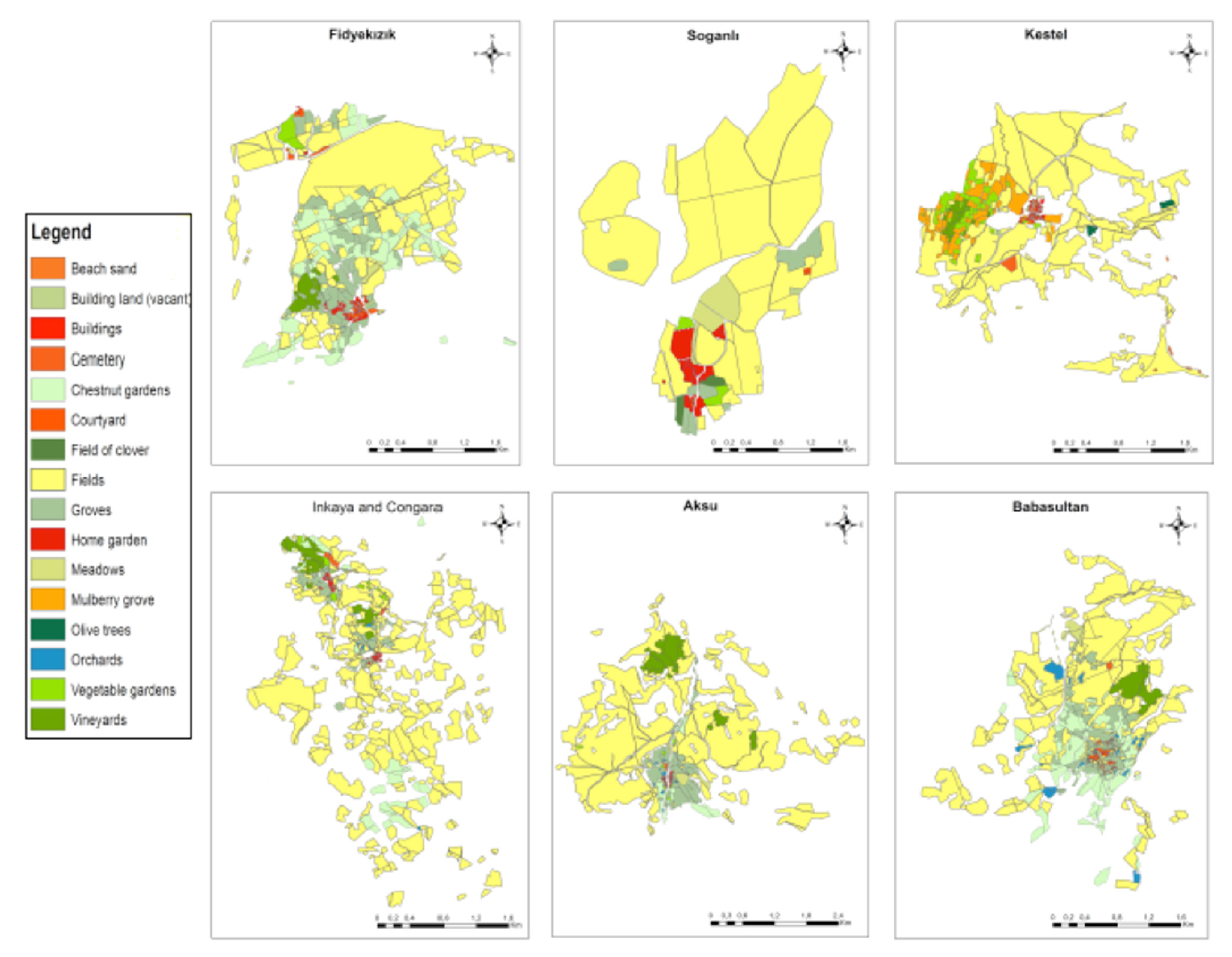
There are no other reliable available series of population registers or censuses for the entire nineteenth century. Bursa as a region did not suffer any major demographic shocks in the 1840s or 1850s. There were also no substantial migration waves in this period, if we leave aside the incoming refugees following the Crimean War (1853–1856) in the late 1850s. This is the reason we are confident our population census data from the 1840s are commensurable and in accord with population levels of the 1850s. For the 1850s, we have detailed cadastral maps of seven villages located in the vicinity of Bursa city available in the Turkish Presidency State Archives of the Republic of Turkey, Department of Ottoman Archives, Map Collection (HRT.h. 561, 562, 564, 565, 566, 567). These detailed maps, with an average scale of 1:2000, provide high-resolution spatial distribution of residential and agricultural land uses for the villages of Aksu, Babasultan, Fidyekızık, Inkaya, Kestel, Soganlı, and Congara (Figure 2). The map collection of the Ottoman Archives was closed to research for decades until its reopening in 2008 after a thorough reorganization. Unfortunately, in this new organization, maps in the collection do not have any metadata or additional documentation and the collection consists solely of maps. The accompanying documentation produced along with the maps is not available. This situation has massive limitations, including for the cadastral maps we used. Their accompanying cadastral registers or any other documentation have been detached from them. There is no research on these maps. Studies on limited Ottoman cadastral activity are also very sparse [63]. We do not know the exact purpose or the extent of the cadastral effort. What we can assume is that these maps were connected to the cadastral map of the city of Bursa prepared after the devastating 1855 earthquake. Although this earthquake caused massive destruction and extensive rebuilding activity for the city [64] there is no indication that it destroyed or changed the residential areas in the countryside. Therefore, we cannot differentiate the land use specificities on the maps. However, in this study we are focusing on the residential areas and therefore, the lack of information on property or usufruct relations are not of central importance. Since the maps delineate both the residential areas as well as the fields of the settlements, we are convinced that they convey the information we need. To the best of our knowledge these maps were only used twice in the literature to estimate approximate maximum walking time distances to cultivated fields from the residential centres and for geosampling purposes [54,65].

In our model, accessibility is an important variable. However, there is no reliable map with accurate detail for connectivity and accessibility of all rural settlements in the region of Bursa produced before the 1940s. The most advanced maps from the late Ottoman Empire are the series produced by the General Staff of the Ottoman Army starting in the 1910s, yet they are not detailed enough to be used in our regional modelling, as they lack rural transport connections. The oldest series of maps suitable for our purposes are the military maps produced by the German General Staff, the Department of Wartime Map and Survey Service during World War II (Deutsche Heereskarte 1:200,000 Türkei) [66]. Although these maps are produced approximately one hundred years later then the period of our examination, among their alternatives they are still the most suitable ones for our modelling.

The segments of the transport infrastructure used for the needs of the agricultural sector in the region, and in the country in general, did not experience any radical change either regarding the road making technologies (no extensive macadam road network) or vehicles used on the roads (mainly ox and horse carts but no wagons) until the 1940s [67]. For the region of Bursa, if we leave aside newly established settlements’ connections, there are only a few exceptions: the Gemlik-Bursa road that was constructed in 1865 [68], and the Mudanya-Bursa railroad completed in 1892 [69]. Both lines were aimed at connecting the city of Bursa with its harbours and did not transform the transport in the region. Gemlik connection was still not suitable for wagons and the Mudanya railway was not connected to the Ottoman Anatolian railways. These are the reasons we assume a static logistical infrastructure between the 1840s and the 1940s in the region.

4. Methods

We used land cover datasets that cover the sampled seven villages (Figure 2) and census data combined with geo-physical, accessibility, location and natural amenities data to produce residential land cover and gridded population distribution maps for Bursa in the 1850s. We used aspect, elevation and slope as geo-physical factors; distance from roads as accessibility-based factors; distance from main settlement centres and village centres as location; distance from the sea, the mountain, water bodies, and lakes as natural amenities. Flat slope, lower elevation and an aspect ratio indicating southern and eastern orientations are highly valued for residential development [70,71]. The steep slopes are costly for residential construction and also susceptible to soil erosion and landslide hazards [72]. Aspects indicating southern and eastern directions are more suitable for residential development given that these are exposed to more sunlight and heat during winter time compared to other orientations. Regarding accessibility, the locations closer to the roads are highly valued due to decreasing costs of transportation of people, goods and services [71]. The zones in the vicinity of village centres and main settlement centres enjoy the economic benefits resulting from agglomeration of commercial uses as well as mixed used land developments [71]. The zones close to natural amenities are highly valued not only for their recreation characteristics but also their provision of ecosystem services to the inhabitants [73].

Five main methodological stages were undertaken: (1) areal extent delineation using population and land cover samples to identify the size of the build-up in the study area; (2) suitability analysis for the detection of potential sites for residential land development through integrating multi criteria analysis (MCA) with fuzzy membership approaches; (3) generating probability maps of residential development through combining residential zones, socio-economic factors, and natural constraints data with the suitability maps; (4) modelling population distribution using probability maps, OLS and GWR regression approaches; and (5) assessing the accuracy of the population distribution models obtained from regression analysis. Figure 3 summarises the whole modelling procedure. All elements of the model will be elaborated in the following sections.

4.1. Reconstruction of Residential Land Cover/Use

4.1.1. Areal Extent Delineation

Historical records from the Ottoman administration during the 1840s do not contain information on the residential areal extent for all of the settlements in the study area. Therefore, the areal extent of each residential area in a settlement (Area_i) was estimated based on a power scaling relationship with its population (Pop_i) [74,75]:

$$Are{a}_i=\alpha Po{p}_i^{\beta }$$

(1)

where α is the coefficient and β is the scaling factor. Concerning Equation (1), a strong relationship was found for different study areas such as Mexico [75] and the US [4]. Different β values were also estimated for the UK (0.375), Japan (0.914), and China (1.38) [76]. Equation (1) was fitted to the data of the seven villages which have spatial land use information (Figure 2) to estimate α and β. The spatial structure of small settlements appear disorganised and are generally characterised by low population density [75]. We have such examples in our study area where low density population was settled in a more spacious land (e.g., Soganlı, Inkaya and Fidyekızık) compared to high density populations settled in a relatively smaller area (see

Table A1. Information on population and area of residential land across seven settlements of Bursa.

Village	Population	Total Area of Residential Land 1 (m2)	Total Area of Agricultural Land 2 (m2)
Aksu	378	38,180	7,785,767
Babasultan	458	45,811	4,582,647
Çonkara	130	27,298	3,703,626
Fidyekızık	200	62,019	2,484,866
Inkaya	130	42,939	1,375,435
Kestel	228	67,887	4,093,205
Soganlı	54	91,695	2,324,190

Note: ¹ Residential buildings and courtyards, cemetery and home gardens. ² Chestnut gardens, olive trees, mulberry groves, orchards, vineyards, fields, field of clover, meadows, and vegetable gardens.

in Appendix A). Therefore, using Equation (1), we estimated two different equations separately for two different types of settlements: the former settlement type represents low density built-up having population less than or equal to 250, and the latter is a high density area with a population greater than 250. Using the estimates of α and β and population data, the areal extent of residential land cover was estimated for all the unknown data points. Similarly, based on the correlation between the known population and land area, the areal extent of agricultural land cover was also estimated for the settlements which lack information. Here are some basic assumptions of the residential reconstruction model:

1. We have the point data in GIS representing the central point of each of the settlement centres of Bursa. It is assumed that built-up land developed outwards from their central point where the central locations were occupied first and the farthest locations were occupied last. The residential areas computed from Equation (1) for each settlement were represented by circular zones that were drawn from the settlement centre outwards (Figure A1 in Appendix A). This is in line with the concentric zone theory of Burgess [77] from 1925, which indicates that as a city develops, it spreads out from the central core.

2. This is also true for the settlements located along the coastal area; but in this case, settlements developed from their centre (that are generally located close to the coastal area) to the inner land areas. Due to physical restrictions, the settlements in the coastal area were developed more densely compared to those located in the mainland.

3. Two models can be distinguished: first, there is high density built-up land where all the residential development takes place within the inner circular zone representing the total area that is built-up (Figure A1). Second, low density development is considered where the radius of the (inner) circle was doubled (shifting from the inner to the outer circular zone in Figure A1). It is observed from the sampling villages that residential development was generally dispersed from its centre to the outer zone by doubling or tripling the radius of the inner circular area.

4.1.2. Non-Inhabitable Land

The land with natural constraints such as water bodies, lakes and areas with elevation higher than 1000 m were regarded as non-inhabitable. For the 1850s, we note that there is no land that was recorded as protected land due to its biological diversity and natural or cultural resources. Although protected areas are considered as non-inhabitable, these were not included in the analysis due to data availability issues. Therefore, only the land with natural constraints were considered as non-inhabitable. The influence coefficient of inhabitability, w_1,x for pixel x was set to zero for non-inhabitable areas and one for inhabitable areas.

4.1.3. Residential Land Use Suitability

The allocation of residential land cover/use can be approached using MCA applications such as land suitability analysis. In the current context, land suitability analysis was applied to develop a probability map and to predict the historical residential land cover dictated by geo-physical parameters such as slope, aspect, elevation, as well as accessibility, location and natural amenities (Figure 4) [78,79].

As can be expected, many factors can be selected for the land studies, and those finally selected are in line with the study objectives, the information available etc. We considered 10 factors grouped into three groups that were evaluated through the AHP as shown in Figure 5. The objective is defined at the top, the three main criteria are at the second level and the corresponding sub-criteria are given at the third level (for an example of the decision hierarchy model for the AHP, see Ustaoglu and Aydınoglu, [73]). The land suitability model (Figure 5) in our study operates vertically, where each criteria map is multiplied with the corresponding weight at the third, second and first level and then all individual results are added to obtain the final suitability map.

AHP is a commonly used method in spatial multi-criteria decision analysis. The pairwise comparison approach developed by Saaty [80] is based on the establishment of hierarchies of relative importance. Each criterion is assigned a value from each class to identify the weights calculated from pairwise comparison matrices. From the pairwise comparison matrix, final values of the factors under each corresponding hierarchy are obtained as well as the consistency ratios (CR), which indicate consistency of the values assigned in each matrix according to Equation (2):

$$\begin{array}{l}CR=\frac{CI}{RI} where\\ CI=\frac{{\lambda }_{\max }-n}{n-1}\end{array}$$

(2)

where λ_max is the principle eigenvalue of the matrix, n is the order of the matrix, CI is the consistency index and RI is the average of resulting CI depending on order n. In Saaty’s [80] explanation, CR less than 0.10 indicates that the pairwise comparison matrix has acceptable consistency, otherwise the matrix includes inconsistencies. In the current study, the CR computed for each pairwise comparison matrix was lower than 0.10, implying that the weight values are consistent (

Table A2. Pairwise comparison matrix of the evaluation criteria for residential suitability.

Criteria	Physical Characteristics	Accessibility and Location	Natural Amenities	Weights
Physical characteristics	1	1/5	3	0.195
Accessibility&location		1	6	0.717
Natural amenities			1	0.088
CR: 0.098
Physical characteristics Sub-criteria	Aspect	Slope	Elevation	Weights
Aspect	1	1/3	2	0.249
Slope		1	3	0.594
Elevation			1	0.157
CR: 0.056
Accessibility&location Sub-criteria	Dist_Roads	Dist_Village centers	Dist_Residential centers	Weights
Dist_Roads	1	1/2	½	0.196
Dist_Village centers		1	½	0.493
Dist_Residential centers			1	0.311
CR: 0.056
Natural amenities Sub-criteria	Dist_Mountains	Dist_Water bodies	Dist_Lakes	Dist_Coastline	Weights
Dist_Mountains	1	1	1	1	0.246
Dist_Water bodies		1	2	1	0.298
Dist_Lakes			1	1	0.21
Dist_Coastline				1	0.246
CR: 0.022

Note: CR: Consistency Ratio.

in Appendix A). Four different scenarios were considered for the suitability assessments. In the first scenario, accessibility and location were given the highest priority in the residential suitability analysis. In Scenarios 2 and 3, physical attributes and natural amenities were of high importance, respectively. In Scenario 4, equal weights were assigned to the three main criteria influencing the residential suitability (see Figure A2 in the Appendix A). The AHP weights computed for each scenario are given in

Table 2. AHP weights of the evaluation criteria for residential suitability.

	AHP Weights
Sub-Criteria	Model 1	Model 2	Model 3	Model 4
Aspect	0.049	0.179	0.022	0.083
Slope	0.116	0.426	0.052	0.198
Elevation	0.031	0.113	0.014	0.052
Dist_Roads	0.141	0.038	0.038	0.065
Dist_Village centers	0.353	0.096	0.096	0.164
Dist_Resident centers	0.223	0.061	0.061	0.104
Dist_Mountains	0.022	0.022	0.176	0.082
Dist_Water bodies	0.026	0.026	0.214	0.099
Dist_Lakes	0.018	0.018	0.151	0.070
Dist_Coastline	0.022	0.022	0.176	0.082

.

For the standardisation of suitability criteria maps, different approaches can be used, including deterministic, probabilistic and fuzzy methods. By contrast to the deterministic approach, it is possible to model concepts with transitional membership with the use of the fuzzy membership method [81]. Conventional maps represent discrete attributes following a Boolean approach resulting in a point, a line or a polygon. Nevertheless, no partial membership exists in the deterministic approach that contradicts with the fuzzy logic, which allows objects or elements to have intermediate values. In the current study, we employed three different models to develop fuzzy membership functions. These are the Gaussian function, the monotonically decreasing sigmoid, and the linear functions. The variable type and fuzzy membership functions for the corresponding criteria are summarised in Figure 6.

The suitability maps created for Scenarios 1 to 4 will be summarised at the end of the results section. In the suitability maps, the values range between 0 and 1, 0 representing the lowest suitability whereas 1 stands for the highest suitability. Following the development of suitability maps, the influence coefficient of suitability, w_2,x for pixel x can be calculated using Equation (3):

$$w_{2,x}=\left[\frac{p_{x,i}}{{\displaystyle \sum _{x=1}^n{p}_{x,i}}}\right]where\hspace{1em}x\in i=(1,\dots ,N)$$

(3)

where p_x,i is the pixel value representing the suitability index of the corresponding pixel x, and i represents each of the settlements in the study area where i = 1,…,590. Equation (3) indicates that suitability index value of each pixel is normalised through dividing each of the pixel value to the sum of total pixel values assigned to each location i. In order to compute the coefficient of suitability, w_2,x, we used the suitability map of Scenario 4, which is based on equal weights of the main criteria, and left other scenarios to be searched in a comparative study in the future work.

4.1.4. Socio-Economic Factors

Following Fang and Jawitz [4], we separated socio-economic factors for urban (U) areas from those for rural (R) areas. We applied the distance decay model, which indicates that residential density decreases with increasing distance from the urban centre. The urban areas comprise the residential settlements in our study, area having populations greater than 1000 people. The distance decay model is in line with the typical urban model in which the density of urban activity follows a declining slope as one moves away the central city [82]. Changes in density across different distances from the city centre reflect a variety of geo-physical and socio-economic factors. The inverse power function was used to represent the distance decay effect on population density from the central core to the outskirts. The influence coefficient of socio-economic factors, w_3,x, for urban pixels (x ∈ U) is given as follows [4]:

$$w_{3,x}=r_{x,i}^{-{\lambda }_i} for\hspace{1em}x\in U$$

(4)

where r_x,i is the radial distance from the central point of residential area i to pixel x, and λ_i is the density gradient for each of the residential area i. Following Chen [83], the density gradient, λ_i, is linked to the scaling factor β from Equation (1). Using Equation (5), λ values were calculated for each settlement i in the study area such as:

$${\lambda }_i=2*(1-\beta )$$

(5)

For rural areas, proximity to main residential centres is advantageous for socio-economic development. We have considered this impact as one of the factors influencing the residential suitability index. Because we used the aforementioned impact in developing the suitability maps, in contrast to Fang and Jawitz [4] we did not compute it separately in order to prevent double counting.

4.2. Population Mapping

4.2.1. Population Mapping Using Probability Maps

Based on high-density and low-density models defined previously, the probability of finding residential land cover under the given assumptions was calculated for all locations using the following equation [4]:

$$P_x=\frac{w_{1,x}{w}_{2,x}{w}_{3,x}}{{\displaystyle {\sum }_{w_{1,x}{w}_{2,x}{w}_{3,x}}}}{P}_Z for\hspace{1em}x\in Z=(U,R)$$

(6)

where Z represents urban (U) or rural (R) pixel; w_1,x, w_2,x, w_3,x are as defined previously. For the distribution of population, it is assumed that the cells having higher probability values are more densely developed compared to those having lower values. Equation (6) was implemented with the use of model builder in ArcGIS to produce the probability maps and historical population datasets.

4.2.2. Population Mapping Using Multivariate Regression Models

Multivariate OLS regression and GWR models were developed to disaggregate the census data from 590 settlements to smaller spatial units of reconstructed residential land cover to provide detailed information on the population locations. The explanatory variables relate to socio-economic conditions, E_i, (e.g., the area of agricultural land that was used as a proxy for the agricultural holdings of the residents; the area of residential land indicating the density of residential development), physical, P_i, (e.g., slope, elevation) and locational characteristics, L_i, (e.g., distance to settlement centres and to main residential centres), accessibility, A_i, (e.g., distance to roads) and natural amenities, N_i, (e.g., distance to lakes, water sources, mountains and the coastal area). Socio-economic conditions represent social resources which attract populations to residential areas. Spatial characteristics (e.g., A_i and L_i) capture locational conditions and geographic advantages of residential land use. The physical attributes indicate that flat surfaces and lower elevation are the most valued for the residential development compared to high slope and high elevation locations. The zones close to natural amenities are the most valued for their development potential regarding the residential land as well as the development potential of green areas in the vicinity of residential land uses. Therefore, the relationship between population, POP_i, and the determinant variables at location i can be written as follows:

$$PO{P}_i=f(E_i,P_i,A_i,L_i,N_i)$$

(7)

We specified the population and explanatory factors relationship as a linear function of the exogenous variables (Equation (7)). Regarding the OLS regression analysis, three different models were developed: Model 1 is based on a selected sample data of population less than or equal to 250; Model 2 focuses on the sample where the population is more than 250; and Model 3 is based on the full sample data representing all the settlements in the study area. To consider multi-collinearity, first we computed pairwise correlation coefficients of the variables, and then the variables with higher correlations were removed.

GWR was developed to explore the determinants of population growth, particularly considering the cases where spatial non-stationary relationships prevail [84]. By contrast to the OLS model, the GWR is carried out using the localised sampling points within a geographic space. It is therefore assumed that depending on location, defined as pairwise coordinates (x,y), the modelled relationship presents variations. The GWR model can be defined as:

$$y_j={\beta }_0(u_j,v_j)+{\displaystyle \sum _{i=1}^p{\beta }_i(u_j,v_j)x_{ij}}+{\epsilon }_j$$

(8)

where (u_j,v_j) represents the coordinates for location j; β₀(u_j,v_j) are the local regression coefficients for independent variables, x_i, at location j. β₀(u_j,v_j) is the intercept and ε_j is the error term. β₀(u_j,v_j) was estimated with the following equation:

$${\beta }_i(u_j,v_j)={\displaystyle \sum _{k=1}^n{w}_{jk}}(y_k-{\beta }_0(u_j,v_j)-{\displaystyle \sum _{i=1}^p{\beta }_i(u_j,v_j)x_{ij}{)}^2}$$

(9)

where w_jk is the distance decay function for location j and k, assuming that observations close to sample point j have a higher impact on local regression parameters. Therefore, regression parameters will have different influence on each specific location given a system of estimations based on geographical weighting. w_jk were calculated using the Gauss function method [84] which is given in Equation (10):

$$w_{jk}=\exp (-d_{jk}^2/b^2)$$

(10)

where d_jk represents the distance between location j and k; and b represents the kernel bandwidth. GWR calculates optimum distance for fixed kernel and optimum number of neighbours for adaptive kernel [85]. The optimal number of nearest neighbours is determined by selecting the model with the lowest Akaike Information Criterion (AIC) score. Regarding fixed kernel, it is assumed that bandwidth at each regression point is constant whereas it is a variable bandwidth for adaptive kernel. In other words, GWR assigns higher weights where data are more scattered and lower weights where data are denser.

Because the results are sensitive to bandwidth, it is necessary to determine the optimum bandwidth [11]. If the bandwidth is known, it can be applied directly. If the bandwidth is unknown, the AIC of minimum discrepancy estimation can be used. For some location i, we obtained negatively estimated population values. Therefore, the local bandwidth were adaptively adjusted to prevent the coefficients from becoming less than zero in the cases where negative population values were predicted (see Chu et al. [21]). We estimated four different models as summarised below:

$$M{1}_{GWR}:Po{p}_i=f(E_i,P_i)$$

(11)

$$M{2}_{GWR}:Po{p}_i=f(E_i,N_i)$$

(12)

$$M{3}_{GWR}:Po{p}_i=f(E_i,P_i,A_i,N_i)$$

(13)

$$M{4}_{GWR}:Po{p}_i=f(E_i,L_i,N_i)$$

(14)

where the variables of E_i, P_i, L_i, A_i and N_i are as defined previously. The variables used in each of these models were selected based on the pairwise correlations given that highly correlated variables were removed from the regressions. The multicollinearity in the GWR models were detected with the ‘condition number’, which evaluates the local multicollinearity. Results associated with condition numbers larger than 30 may be unreliable. From Equations (11) to (14), the estimations of condition numbers were smaller than 30 indicating that multicollinearity is not an issue for the estimated models.

4.2.3. Model Validation

The model validation was undertaken using two measures as well as the Moran’s I index was used. Firstly, we computed root mean square error (RMSE) and total absolute error (TAE). The TAE is a measure of the total error observed in the study area while RMSE measures average deviation produced in the study area. The formulas are given below where P_i and P′_i are the observed and predicted values of population in location i, and n is the total number of settlements.

$$RMSE={\left[n^{-1}{\displaystyle \sum _{i=1}^n{\left|{P^{\prime }}_i-P_i\right|}^2}\right]}^{1/2}$$

(15)

$$TAE=\left(\frac{{\displaystyle \sum _{i=1}^n\left|{P^{\prime }}_i-P_i\right|}}{{\displaystyle \sum _{i=1}^n{P}_i}}\right)\times 100$$

(16)

Moran’s I statistic (Moran [86]) indicates whether the data is clustered, dispersed or randomly distributed. A statistically significant positive Moran’s Index implies a spatial clustering while a negative Moran’s I index indicates dispersion. To test for autocorrelation effects, we applied Moran’s Index to the estimated residuals of both models of OLS and GWR.

5. Results

5.1. Historic Residential Reconstructions

Two different historical reconstructions were undertaken using Equation (6); one based on the high density residential land use model and other based on the low density model. Figure 7 presents the different results of these two reconstructions for the 1850s, which were developed as 30 × 30 m raster maps. The former model resulted in smaller areas(i.e. around 25% area of the latter model) due to the assumption of compact development patterns, which contradicts with the dispersed pattern adopted in the latter model. By using the high density model, the total amount of residential land was 0.36% of the total area. Contrary to that, the ratio becomes 1.45% with the low-density model.

The estimated coefficients and scaling factors indicating the relationship between population and size of the residential area are given in Equations (17) and (18). We note that there is a negative relationship with the area and population for the smaller settlements whereas the relationship becomes positive for the larger settlements with a population greater than 250.

$$\begin{array}{l}Are{a}_{i,residential}=277,552.4\left[m^2\right]\times Po{p}_i^{-0.29625}\\ R^2=0.96\end{array}$$

(17)

$$\begin{array}{l}Are{a}_{i,residential}=3936.749\left[m^2\right]\times Po{p}_i^{0.39344}\\ R^2=0.99\end{array}\mathrm{for} \mathrm{each} \mathrm{area} (i) \mathrm{of} {\mathit{Pop}}_i>250$$

(18)

Based on these findings, we examined the spatial distribution of population and population density in the Bursa region. Accordingly, the three most urbanised areas are the Bursa city, Mihaliç and Gemlik, which have populations of 30,968, 6258 and 3364, respectively. The population growth observed in the area has led to development of settlement agglomerations across the study area, particularly located in the coastal area (Tirilye, Kumyaka, Mudanya, Umurbey, Dürdane, Gemlik), along water streams (Alaylı, Yenisehir, Adibini, Cerrah, Gölyazı, Kayapa, Görükle) and İznik Lake (Benli, Sölöz, Yenicihan, Çakırlı), and on the southern plains of Uludag (Cekirge, İsabey, Tepecik, Bursa city). We also note that there are high density settlements mainly located in the mountainous areas around the bodies of water and along the coastal line. The reasons for these population dynamics might be the favourable climate and the geophysical conditions and attractiveness of natural attributes to the residents of these settlements. The details of reconstructed maps are provided in Figure 8, which compares the differences between simulated and observed residential land cover for the sampled villages where spatial data on land cover/use exist. It is noted that the observed population is well represented with the low-density model because the observed residential land is more dispersed compared to the simulated land cover of the high-density model. Given this, population distribution analysis from regression models in the next section will be based on the low-density model.

5.2. Results of Population Distribution and Validation

The estimated relationship between population and the determinant factors obtained from OLS is given in

Table 3. Estimates from the OLS regression model.

	Model OLS1: Pop ≤ 250)		Model OLS2: Pop > 250)		Model OLS3: Pop > 0
	Model 1a	Model 1b	Model 2a	Model 2b	Model 3a	Model 3b
	Coefficient	Coefficient	Coefficient	Coefficient	Coefficient	Coefficient
Constant	350.957 ** (10.43)	350.591 ** (8.15)	−4169.14 ** (507.76)	−3962.24 ** (385.21)	−1770.97 ** (102.79)	−1824.86 ** (70.28)
Elevation	0.007(0.01)	-	−1.053 * (0.61)	-	−0.071(0.11)	-
Slope	0.379(0.41)	0.619 * (0.33)	42.626 * (27.55)	-	3.144(4.72)	-
Dist_roads	0.003(0.01)	-	−0.572 * (0.35)	−0.573 * (0.32)	−0.059(0.06)	-
Dist_res_cent	−0.001 * (0.01)	−0.0003 ** (0.01)	0.011(0.01)	-	0.002(0.00)	-
Dist_village_cent	0.001(0.00)	-	0.243(0.20)	0.247 *(0.18)	0.023(0.04)	-
Dist_lakes	−0.0001(0.00)	-	−0.003(0.01)	-	−0.0002(0.00)	-
Dist_sea	−0.0001(0.00)	-	0.005(0.01)	-	0.001(0.00)	0.003 ** (0.00)
Dist_mountain	−0.0001(0.00)	-	−0.024 ** (0.01)	−0.024 ** (0.01)	−0.003(0.00)	-
Dist_water	−0.0002(0.00)	-	−0.027 ** (0.01)	−0.021 ** (0.01)	−0.011 ** (0.01)	−0.009 ** (0.00)
Res_land	−0.003 ** (0.00)	−0.003 ** (0.00)	0.109 ** (0.00)	0.109 ** (0.00)	0.015 ** (0.00)	0.015 ** (0.01)
Agri_land	−1.003 ** (0.00)	−1.006 ** (0.00)	0.001(0.00)	-	0.0002 ** (0.00)	0.0003 ** (0.00)
Dependent var.	Pop	Pop	Pop	Pop	Pop	Pop
Sample size	432	432	158	158	590	590
R-squared	0.73	0.74	0.79	0.79	0.89	0.9
F-stat	107.09 **	296.59 **	50.70 **	112.17 **	458.93 **	1267.69 **

Note: In paranthesis are the standard errors; * significant at 10%; ** significant at 5%; Res_land: Total residential land area of the corresponding village in square meters; Agri_land: Total agricultural land area of the corresponding village in square meters.

. Although the results of R² and F-statistics indicated that Model 3 is the best performing model among others, Model 1 shows the lowest overall estimation errors (see Figure A3 in Appendix A). We have negative outlier points identified in the boxplot indicating that population was underestimated for some settlements whereas it was overestimated for others associated with positive outlier points (Figure A3). Although Model 3 is the most comprehensive model comprising all the settlements and the favourable results obtained from R² statistics, we used Models 1 and 2 due to their low estimation errors for the prediction and distribution of population to the fine scale raster cells.

The statistics obtained from GWR estimates are given in

Table 4. Statistics from the GWR model estimations.

	Model GWR 1	Model GWR 2	Model GWR 3	Model GWR 4
Dependent var.	Population	Population	Population	Population
Explanatory var.	Elevation, Res_land_area	Dist_lakes, Dist_water, Res_land_area	Slope, Dist_roads, Dist_lakes, Dist_sea, Dist_watercourses, Res_land, Agri_land	Dist_village_centers, Dist_lakes, Dist_watercourses, Res_land, Agri_land
Neighbours	30	20	25	20
Effective number 1	181.204	230.072	12.093	10.688
Sigma 2	610.21	514.55	67.855	110.444
AIC	9352.28	7321.08	270.31	255.09
R2	0.86	0.94	0.98	0.93
R2 adjusted	0.79	0.88	0.96	0.74

Notes: ¹ This indicates a tradeoff between the variance of the fitted values and the bias in the coefficient estimates and is related to the choice of the bandwidth. For very large bandwidths, the effective number of coefficients approaches the actual number; local coefficient estimates will have a small variance but will be biased and vice versa. ² This is the square root of the normalised residual sum of squares. This is the estimated standard deviation for the residuals. Sigma is used for AIC computations. Smaller values of sigma are preferred.

. Model GWR3 is the best model given that sigma and AIC are the smallest; and R² and R²-adjusted are the largest among other models. This is also confirmed in the box plot given that Model 3

And Model 4 showed the lowest overall estimation errors compared to other models (Figure A4 in Appendix A). Therefore, Model GWR3 was used for the spatial distribution of population to the residential cells. The spatial distribution of errors for both OLS and GWR models are presented in Figure 9 and Figure 10.

From Figure 9, estimation errors are the smallest for the settlements of populations less than 250 (Model OLS1). When settlements having populations greater than 250 were included in the regressions, we acknowledge that estimation errors have considerably increased (e.g., Model OLS2 and Model OLS3). The largest estimation errors were observed for the settlements located around the watercourses and those close to mountainous areas. The error is more homogeneously distributed in the case of Model OLS3, which includes all the settlements in the sample.

From Figure 10, the highest estimation errors were obtained from Models GWR1 and GWR2 where the estimated errors were distributed homogeneously in the study area. Models GWR3 and GWR4 showed the lowest estimation errors, which were distributed more heterogeneously compared to the former models. The highest estimation errors were observed for the settlements in the vicinity of Bursa city located on the southern plains of Uludag, and close to residential centres (i.e., population > 1000) which are located along the coastal area, on the western coast of İznik Lake, and along the water courses, mainly in the eastern and western parts of the Bursa region. The lowest error estimations were obtained for the rest of the study area, implying that socio-economic and physical characteristics, accessibility, and natural amenities were influential in the estimation of population in the subject locations.

The population distribution maps created from the probability maps and regression models are shown in Figure 11. A closer look at the values at pixel level shows that pixel values differ due to different estimation methods used for population prediction.

The validation of regression models was done by comparing the population records at the settlement level with the population estimates of the grids reported for each settlement (e.g., the sum of all pixel population values for each settlement). From the TAE and RMSE statistics computed for both OLS and GWR models, RMSE ranges between 0.19 and 91.5 for the OLS and between 7.13 and 40.22 for the GWR models (

Table 5. Model validation results.

	RMSE	TAE
Model OLS 1a	1.327	0.211
Model OLS 1b	2.239	0.211
Model OLS 2a	0.192	0.102
Model OLS 2b	32.118	0.936
Model OLS 3a	86.253	1.231
Model OLS 3b	91.534	1.226
Model GWR 1	7.138	1.044
Model GWR 2	40.224	0.98
Model GWR 3	7.437	0.831
Model GWR 4	9.487	0.825

Notes: RMSE: Root mean square error; TAE: Total absolute error.

). Because it is shown that TAE is more robust to skewed distributions compared to RMSE [87], as it is the case for population density distributions, we will focus on TAE statistics as the main indicator of model performance. Regarding OLS models, Model OLS2a perform better than other OLS models and the worst results were obtained for Model OLS2b. Regarding the GWR, Model GWR3 and Model GWR4 perform better than other GWR models and the worst model was GWR1. From TAE statistics, it can be inferred that GWR models perform better than OLS models. This confirms the findings of the literature which indicated that GWR is more accurate than OLS models, as the latter do not consider the spatial variation of coefficients.

The results from Moran’s I statistic for the OLS and GWR models are shown in

Table 6. Results from spatial autocorrelation statistics for the OLS models.

	OLS M1a	OLS M1b	OLS M2a	OLS M2b	OLS M3a	OLS M3b
Moran’s Index	0.5119	0.4329	0.2872	0.9174	0.5274	0.3803
Z-score	0.9407	0.7967	1.6716	4.686	0.9995	0.7217
p Value	0.3468	0.4256	0.0945	0.0000	0.3175	0.4704

Note: The values are based on inverse distance.

and

Table 7. Results from spatial autocorrelation statistics for the GWR models.

	GWR M1	GWR M2	GWR M3	GWR M4
Moran’s Index	−0.0728	−0.0855	−0.101	−0.0238
Z-score	−0.1348	−0.1586	−0.1879	−0.0418
p Value	0.8927	0.8739	0.8509	0.9665

Note: The values are based on inverse distance.

, respectively. Regarding OLS models, Moran’s I is ranging between 0.28 and 0.91 indicating spatial autocorrelation for the models OLS M2a and OLS M2b. For the other models (Table 6), there is no spatial autocorrelation detected. Regarding GWR models, Moran’s I ranges between −0.101 and −0.023 with p-values of 0.850 and 0.966, meaning that the null hypothesis is not rejected i.e. the spatial variables are randomly distributed (Table 7). Finally, the overall presentation of spatial analysis and population modelling work is given in Figure 12.

6. Discussion

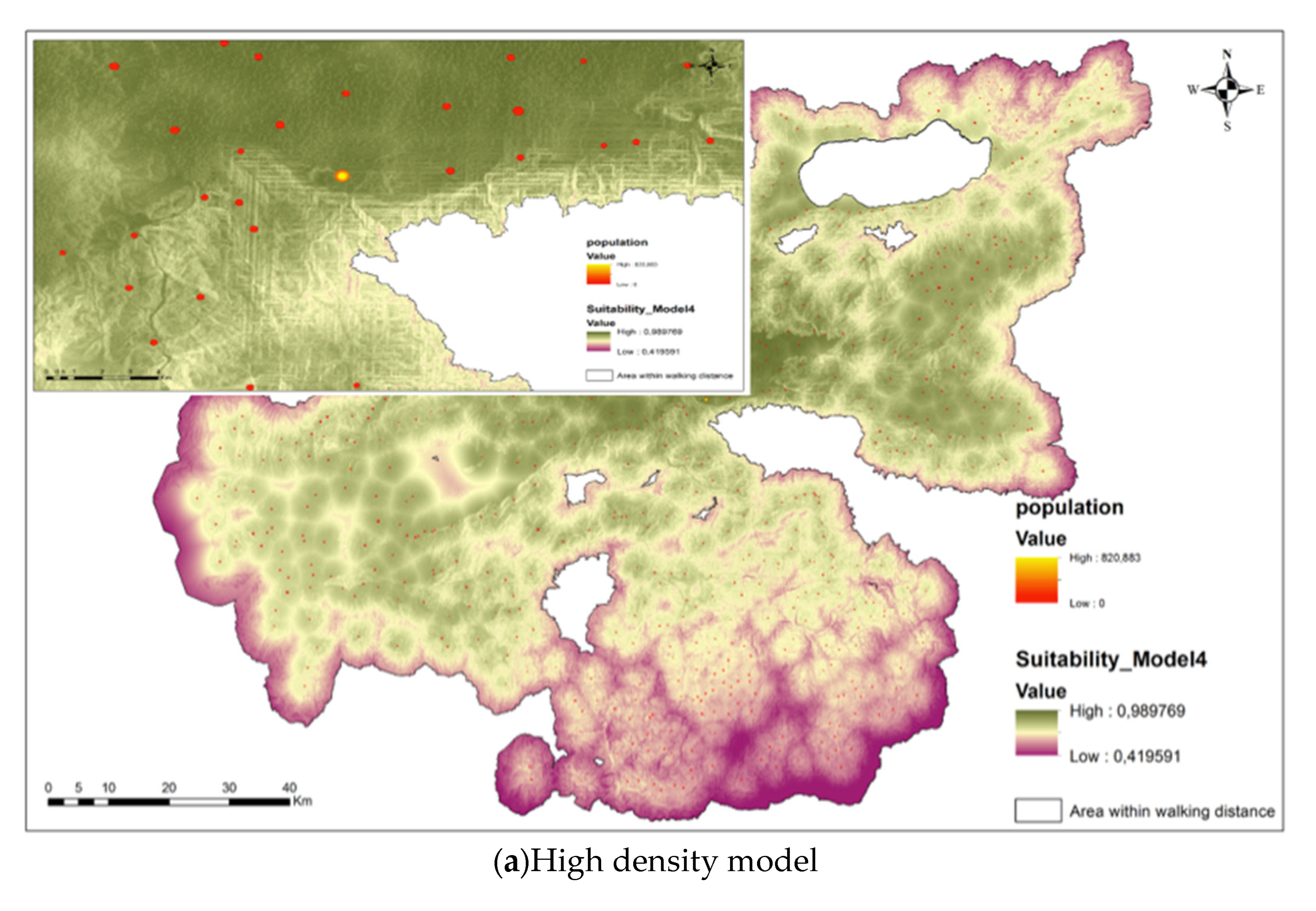
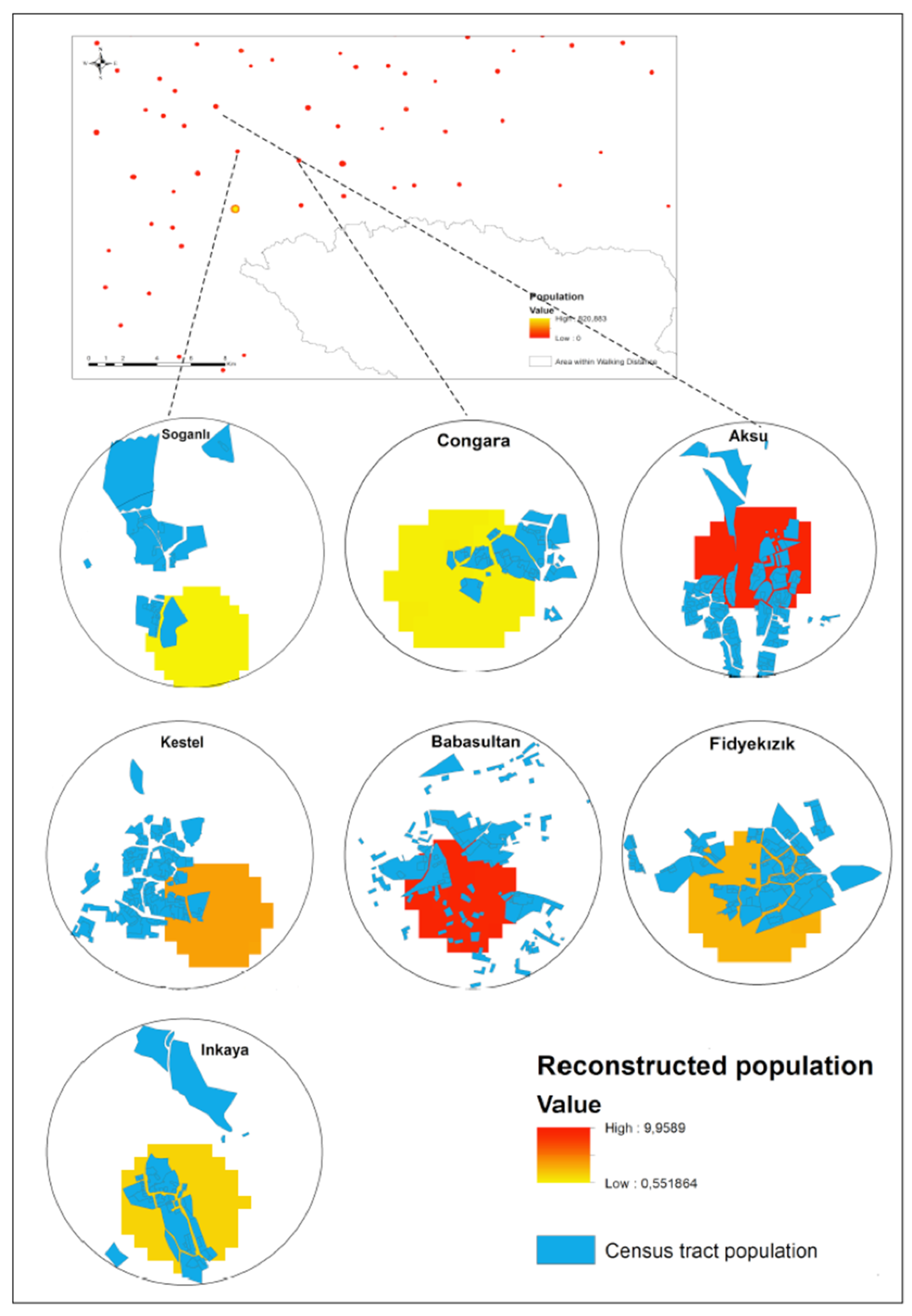
Using the historical census data, cadastral maps of seven villages and other ancillary data (geo-physical, accessibility and location factors, natural constraints and natural amenities), we developed two different probability maps of residential development i.e. compact versus dispersed land use patterns to create a high resolution historical reconstruction of residential land use/cover in the Bursa region in the 1850s. A common method to test the reliability of historical reconstructions is to compare the reconstructions with the information from independent sources [53,88]. Detailed historical maps serve for this purpose, and we compared the model results with the cadastral maps of seven villages, which are the only available historical sources obtained from the Ottoman archives. According to map comparisons (Figure 8), we noted that the pattern of residential land use in the seven villages is more dispersed rather than compact, nevertheless both cases were considered in the modeling of historical reconstructions. Therefore, we concluded that the compact model of historical reconstructions poorly explains the real situation, and dispersed modelling outcomes are more successful in representing the residential land cover/use in the 1850s. Given that the data on historical cadastral maps of the remaining settlements in Bursa region is missing in the archives, we were not able to develop the land use map of the region in digitized form from cadastral maps but attempted to develop probability maps of residential development with an assumption of compact and dispersed development patterns. The validation of historical reconstructions is therefore based on comparisons with information from the cadastral maps of seven villages, and our modelling outcomes for the rest of the villages were not validated due to missing historical information. Land use/cover changes can be projected backward on the basis of existing time series information on the spatial distribution of land cover/use and the driving forces of, and parameters associated with, the land use changes. Regarding the Bursa region, there is hardly any land cover/use map before the 1990s, and due to existence of limited time series spatial maps, we were not able to project land cover/use changes backward [49,89]. Neither we were able to simulate historical land uses through the application of a historical land use reconstruction model [53,90,91]. Despite the limitations of data and methodological framework, the reconstructed residential land cover/use map in the current study can serve as an input in future studies that aim to analyse long term land use changes in the Bursa region.

We followed two approaches for the spatial distribution of historical populations on the reconstructed historical raster maps. The first approach was based on a linear relationship with the probability map. This model requires construction of a residential development probability map through the application of natural constraints, land zoning, socio-economic factors and residential suitability. The second approach used a regression analysis approach (OLS vs. GWR) which redistributed the population on reconstructed raster cells. Because we assumed a positive linear relationship with the probability map, there is no error analysis applicable to this model. The error analysis from the second approach, on the other hand, indicated that Models OLS1a, OLS2a, GWR3 and GWR4 resulted in the smallest errors. From TAE statistics, we found that GWR models perform better than OLS models. This confirms the findings in the literature [22,92,93,94,95], as GWR considers spatial non-stationarity from the reconstructed residential land cover/use map. The gridded population distribution maps obtained using the GWR approach can be used to analyse spatio-temporal patterns of population density in the Bursa region and can be used as an input in future studies focusing on exploring population dynamics in Turkey.

7. Conclusions

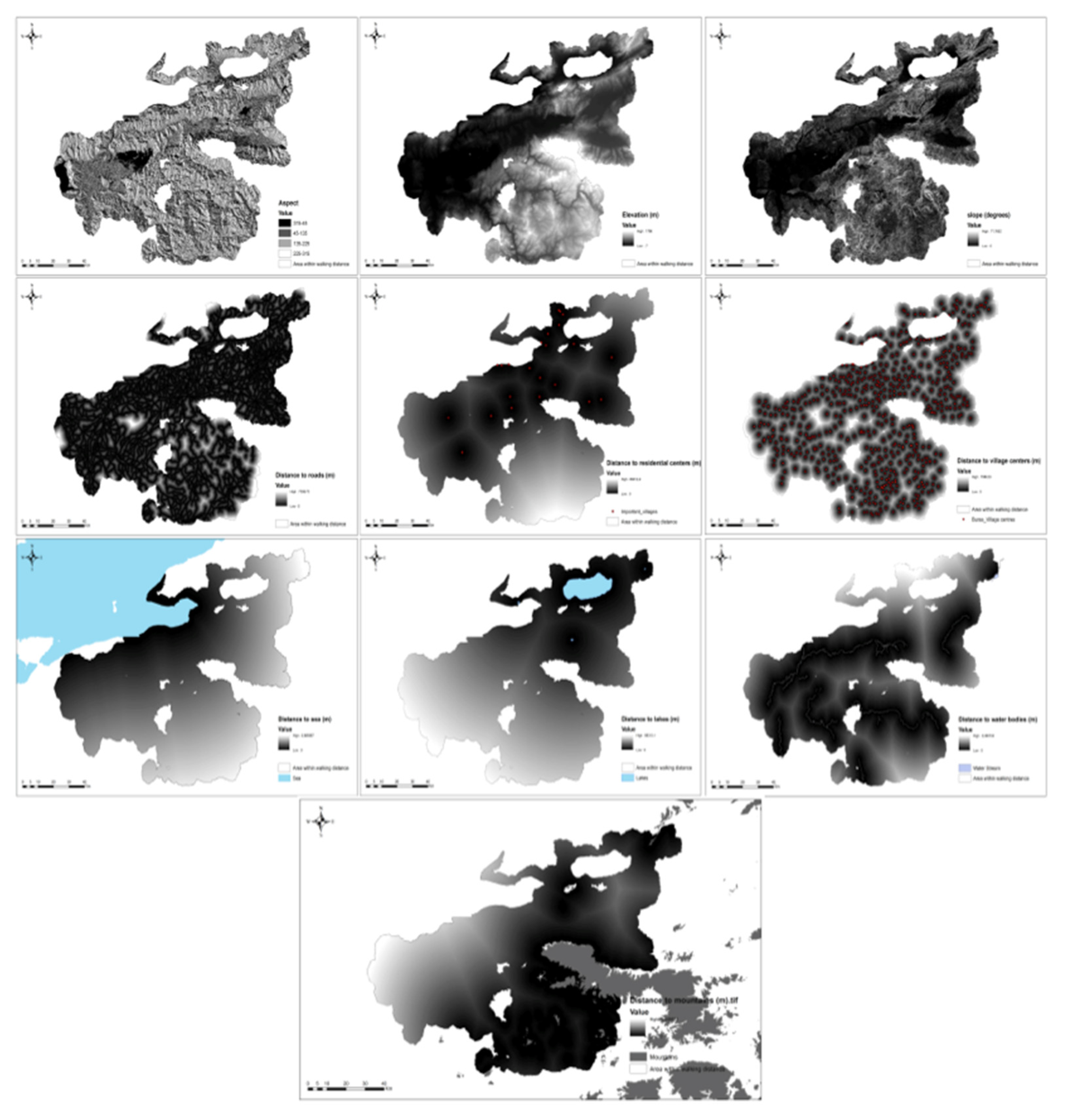
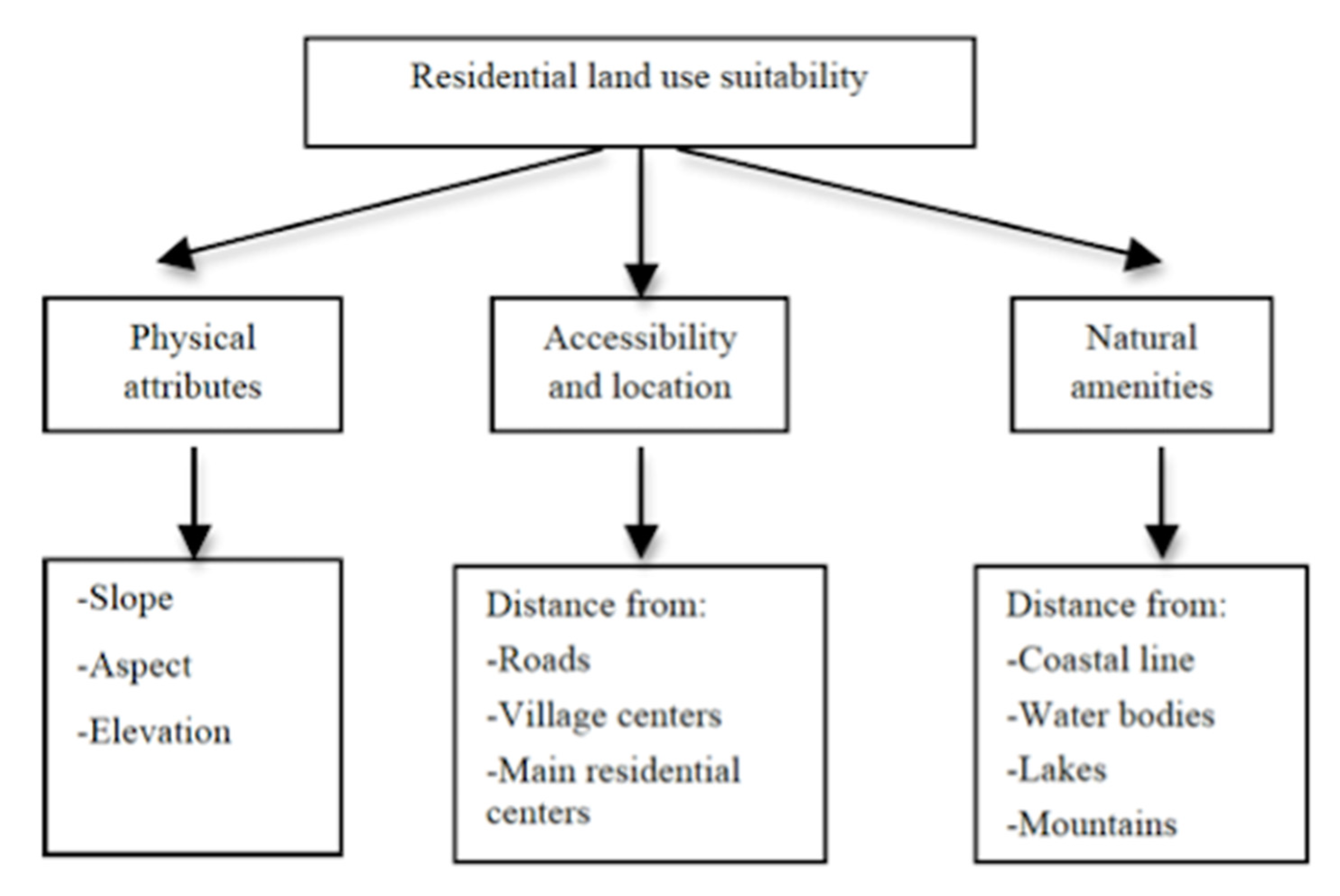
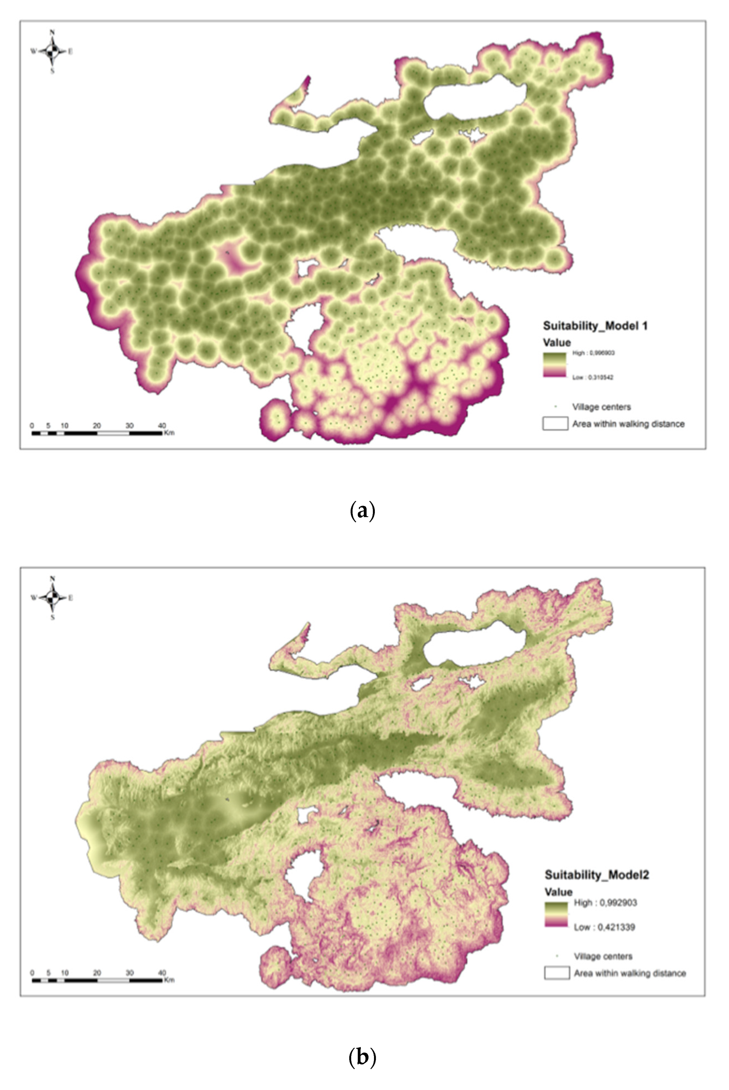
Based on the historical population census data and detailed settlement extents of some sampled villages, this study developed residential land cover maps that were combined with different statistical models of high-resolution population distribution in the Bursa region in the mid-1800s. The reconstruction of residential land cover is based on natural constraints, land zoning, residential suitability, and socio-economic factors, which can be considered as influencing factors that have contributed to the accuracy of final map products. We selected three main criteria, including physical factors, location and accessibility, and natural amenities for the suitability mapping of residential development, which were classified using the fuzzy membership functions and weighted using the AHP method. The integration of fuzzy membership with AHP is an advancement for the analysis of land suitability, and in this way our study contributes to the previous studies which considered deterministic approaches, fuzzy membership, or AHP alone for land suitability modelling.

In the current study, we adopted the low-density residential land cover maps as ancillary data to create historic population grid maps for the Bursa region. The validation analysis that allowed a systematic comparison of the resulting grid population maps with the reference data were utilized for specifying population disaggregation accuracies of the regression models. In the current study, the GWR model has provided the highest accuracies, as the model considers spatial non-stationary. This contrasts with the global OLS model which does not consider spatial heterogeneity. The approach can be used as an input for future studies for the analysis of land cover/use change dynamics and for comparative work of high-resolution population distribution studies regarding the Bursa region and other study areas.

References

1. Pongratz, J.; Reick, C.; Raddatz, T.; Claussen, M. A reconstruction of global agricultural areas and land cover for the last millennium. Glob. Biogeochem. Cycles 2008, 22, GB3018. [Google Scholar] [CrossRef]
2. Yuanyuan, Y.; Shuwen, Z.; Jiuchun, Y.; Liping, C.; Kun, B.; Xiaoshi, X. A review of historical reconstruction methods of land use/land cover. J. Geogr. Sci. 2014, 24, 746–766. [Google Scholar]
3. Kumar, S.; Merwade, V.; Suresh, P.; Rao, C.; Pijanowski, B.C. Characterizing long-term land use/cover change in the United States from 1850 to 2000 using a non-linear bi-analytical model. AMBIO 2013, 42, 285–297. [Google Scholar] [CrossRef] [PubMed] [Green Version]
4. Fang, Y.; Jawitz, J.W. High-resolution reconstruction of the United States human population distribution, 1790 to 2010. Sci. Data 2018, 5, 180067. [Google Scholar] [CrossRef] [PubMed] [Green Version]
5. Liu, X.; Liang, X.; Li, X.; Xu, X.; Ou, J.; Chen, Y.; Li, S.; Wang, S.; Pei, F. A future land use simulation model (FLUS) for simulating multiple land use scenarios by coupling human and natural effects. Landsc. Urban Plan. 2017, 168, 94–116. [Google Scholar] [CrossRef]
6. Perpina Castillo, C.; Coll Aliaga, E.; Lavalle, C.; Martinez Llario, J.C. An assessment and spatial modelling of agricultural land abandonment in Spain (2015–2030). Sustainability 2020, 12, 560. [Google Scholar] [CrossRef] [Green Version]
7. Setyo Darmanto, N.; Galang Varquez, A.C.; Kawano, N.; Kanda, M. Future urban climate projection in a tropical megacity based on global climate change and local urbanization scenarios. Urban Clim. 2019, 29, 100482. [Google Scholar] [CrossRef]
8. Huo, H.; Wang, M.; Zhang, X.; He, K.; Gong, H.; Jiang, K.; Jin, Y.; Shi, Y.; Yu, X. Projection of energy use and greenhouse gas emissions by motor vehicles in China: Policy options and impacts. Energy Policy 2012, 43, 37–48. [Google Scholar] [CrossRef]
9. Shabani, F.; Ahmadi, M.; Kumar, L.; Solhjouy-Fard, S.; Tehrany, M.S.; Shabani, F.; Kalantar, B.; Esmaeili, A. Invasive weed species threats’ to global biodiversity: Future scenarios of changes in the number of invasive species in a changing climate. Ecol. Indic. 2020, 116, 106436. [Google Scholar] [CrossRef]
10. Lambin, E. Modelling and monitoring land-cover change processes in tropical regions. Prog. Phys. Geogr. Earth Environ. 1997, 21, 375–393. [Google Scholar] [CrossRef]
11. Jaimes, N.B.P.; Sendra, J.B.; Delgado, M.G.; Plata, R.F. Exploring the driving forces behind deforestation in the state of Mexico (Mexico) using geographically weighted regression. Appl. Geogr. 2010, 30, 576–591. [Google Scholar] [CrossRef]
12. Ustaoglu, E.; Williams, B. Determinants of urban expansion and agricultural land conversion in 25 EU countries. Environ. Manag. 2017, 60, 717–746. [Google Scholar] [CrossRef] [PubMed]
13. Verburg, P.H.; van Eck Ritsema, J.; de Nijs, T.; Dijst, M. Determinants of land-use change patterns in the Netherlands. Environ. Plan. B 2004, 31, 125–150. [Google Scholar] [CrossRef] [Green Version]
14. Ustaoglu, E.; Aydınoglu, A.C. Regional variations of land-use development and land-use/cover change dynamics: A case study of Turkey. Remote Sens. 2019, 11, 885. [Google Scholar] [CrossRef] [Green Version]
15. Verburg, P.H.; Crossman, N.; Ellis, E.C.; Heinimann, A.; Hostert, P.; Mertz, O.; Nagendra, H.; Sikor, T.; Erb, K.-H.; Golubiewski, N.; et al. Land system science and sustainable development of the earth system: A global land project perspective. Anthropocene 2015, 12, 29–41. [Google Scholar] [CrossRef] [Green Version]
16. EEA. Land-Use Scenarios for Europe: Qualitative and Quantitative Analysis on a European Scale; European Environment Agency (EEA): Luxembourg, 2007.
17. Lung, T.; Lubker, T.; Ngochoch, J.K.; Schaab, G. Human population distribution modelling at regional level using very high resolution satellite imagery. Appl. Geogr. 2013, 41, 36–45. [Google Scholar] [CrossRef]
18. Martin, D. Directions in population GIS. Geogr. Compass 2011, 5, 655–665. [Google Scholar] [CrossRef]
19. Mennis, J. Generating surface models of population using dasymetric mapping. Prof. Geogr. 2003, 55, 31–42. [Google Scholar]
20. Behar, C. The Population of the Ottoman Empire and Turkey, 1500–1927; T.C. Başbakanlık Devlet İstatistik Enstitüsü: Ankara, Turkey, 1996. [Google Scholar]
21. Chu, H.-J.; Yang, C.-H.; Chou, C.C. Adaptive non-negative geographically weighted regression for population density estimation based on nighttime light. Int. J. Geo-Inf. 2019, 8, 26. [Google Scholar] [CrossRef] [Green Version]
22. Roni, R.; Jia, P. An optimal population modelling approach using Geographically Weighted Regression based on high-resolution remote sensing data: A case study in Dhaka city, Bangladesh. Remote Sens. 2020, 12, 1184. [Google Scholar] [CrossRef] [Green Version]
23. Stevens, F.R.; Gaughan, A.E.; Linard, C.; Tatem, A.J. Disaggregating census data for population mapping using random forests with remotely-sensed and ancillary data. PLoS ONE 2015, 10, e0107042. [Google Scholar] [CrossRef] [Green Version]
24. Song, D.-X.; Huang, C.; Sexton, J.O.; Channan, S.; Feng, M.; Townshend, J.R. Use of Landsat and Corona data for mapping forest cover change from the mid-1960s to 2000s: Case studies from the Eastern United States and Central Brazil. ISPRS J. Photogramm. Remote Sens. 2015, 103, 81–92. [Google Scholar] [CrossRef] [Green Version]
25. Belward, A.S.; Skoien, J.O. Who launched what, when and why; trends in global land-cover observation capacity from civilian earth observation satellites. ISPRS J. Photogramm. Remote Sens. 2014, 103, 115–128. [Google Scholar] [CrossRef]
26. Fuchs, R.; Herold, M.; Verburg, P.H.; Clevers, J.G.P.W.; Eberle, J. Gross changes in reconstructions of historic land cover/use for Europe between 1900 and 2010. Glob. Chang. Biol. 2015, 21, 299–313. [Google Scholar] [CrossRef]
27. Long, Y.; Jin, X.; Yang, X.; Zhou, Y. Reconstruction of historical arable land use patterns using constrained cellular automata: A case study of Jiangsu, China. Appl. Geogr. 2014, 52, 67–77. [Google Scholar] [CrossRef]
28. Zhu, F.; Cui, X.F.; Miu, L.J. China’s spatially-explicit historical land-use data and its reconstruction methodology. Prog. Geogr. 2012, 31, 1563–1573. [Google Scholar]
29. Ramankutty, N.; Foley, J.A. Estimating historical changes in global land cover: Croplands from 1700 to 1992. Glob. Biogeochem. Cycles 1999, 13, 997–1027. [Google Scholar] [CrossRef]
30. Klein Goldewijk, K.; Breusen, A.; Janssen, P. Long-term dynamic modelling of global population and built-up area in a spatially explicit way: HYDE 3.1. Holocene 2010, 20, 565–573. [Google Scholar] [CrossRef] [Green Version]
31. Hurtt, G.C.; Frolking, S.; Fearon, M.G.; Moore, B.; Shevliakova, E.; Malyshev, S.; Pacala, S.W.; Houghton, R.A. The underpinnings of land-use history: Three centuries of global gridded land-use transitions, wood-harvest activity, and resulting secondary lands. Glob. Chang. Biol. 2006, 12, 1208–1229. [Google Scholar] [CrossRef]
32. Olofsson, J.; Hickler, T. Effects of human land-use on the global carbon cycle during the last 6000 years. Veg. Hist. Archaeobotany 2008, 17, 605–615. [Google Scholar] [CrossRef] [Green Version]
33. Kaplan, J.O.; Krumhardt, K.M.; Zimmermann, N.E. The effects of land use and climate change on the carbon cycle of Europe over the past 500 years. Glob. Chang. Biol. 2012, 18, 902–914. [Google Scholar] [CrossRef]
34. Ge, Q.; Dai, J.; He, F.; Zheng, J.; Man, Z.; Zhao, Y. Study on cultivated land quantity change and driving factors in some provinces in China over the past 300 years. Nat. Sci. Bullet. 2003, 13, 825–832. [Google Scholar]
35. Zhang, X.; Wang, W.-C.; Fang, X.; Ye, Y.; Li, B. Vegatation of Northeast China during the late seventeenth to early twentieth century as revealed by historical documents. Reg. Environ. Chang. 2011, 11, 869–882. [Google Scholar] [CrossRef]
36. Fensham, R.J.; Fairfax, R.J. The use of the land survey record to reconstruct pre-European vegetation patterns in the Darling Downs, Quensland, Australia. J. Biogeogr. 1997, 24, 827–836. [Google Scholar] [CrossRef]
37. Bolliger, J.; Schulte, L.A.; Burrows, S.N.; Sickley, T.A.; Mladenoff, D.J. Assessing ecological restoration potentials of Wisconsin (USA) using historical landscape reconstructions. Restor. Ecol. 2004, 12, 124–142. [Google Scholar] [CrossRef]
38. Brown, D.G. Mapping historical forest types in Baraga County Michigan, USA, as fuzzy sets. Plant Ecol. 1998, 134, 97–111. [Google Scholar] [CrossRef]
39. Schulte, L.A.; Mladenoff, D.J.; Nordheim, E.V. Quantitative classification of a historic northern Wisconsin (U.S.A.) landscape: Mapping forests at regional scale. Canad. J. Forest Res. 2002, 32, 1616–1638. [Google Scholar] [CrossRef]
40. Foster, D.R. Land-use history (1730–1990) and vegetation dynamics in central New England, USA. J. Ecol. 1992, 80, 753–772. [Google Scholar] [CrossRef]
41. Kaim, D.; Kozak, J.; Kolecka, N.; Ziółkowska, E.; Ostafin, K.; Ostapowicz, K.; Gimmi, U.; Munteanu, C.; Radeloff, V.C. Broad scale forest cover reconstruction from historical topographic maps. Appl. Geogr. 2016, 67, 39–48. [Google Scholar] [CrossRef]
42. Depuydt, F. The large scale mapping of Belgium, 1800–1850. Imago Mundi 1975, 27, 23–26. [Google Scholar] [CrossRef]
43. Gosheva, S.; Walthert, L.; Niklaus, P.A.; Zimmermann, S.; Gimmi, U.; Hagedorn, F. Reconstruction of historic forest cover changes indicates minor effects on carbon stocks in Swiss forest soils. Ecosystems 2017, 20, 1512–1528. [Google Scholar] [CrossRef]
44. Axelsson, A.-L.; Östlund, L.; Hellberg, E. Changes in mixed deciduous forests of boreal Sweden 1866–1999 based on interpretation of historical records. Landsc. Ecol. 2002, 17, 403–418. [Google Scholar] [CrossRef]
45. Godet, L.; Thomas, A. Three centuries of land cover changes in the largest French Atlantic wetland provide new insights for wetland conservation. Appl. Geogr. 2013, 42, 133–139. [Google Scholar] [CrossRef]
46. Feurdean, A.; Munteanu, C.; Kuemmerle, T.; Nielsen, A.B.; Hutchinson, S.M.; Ruprecht, E.; Parr, C.; Perşoiu, A.; Hickler, T. Long-term land-cover/use change in a traditional farming landscape in Romania inferred from pollen data, historical maps and satellite images. Reg. Environ. Chang. 2017, 17, 2193–2207. [Google Scholar] [CrossRef] [Green Version]
47. Antrop, M. The transformation of the Mediterranean landscapes: An experience of 25 years of observations. Landsc. Urban Plan. 1993, 24, 3–13. [Google Scholar] [CrossRef]
48. Carni, A.; Jarnjak, M.; Ostir-Sedej, K. Past and present forest vegetation in NE Slovenia derived from old maps. Appl. Veg. Sci. 1998, 1, 253–258. [Google Scholar] [CrossRef]
49. Petit, C.; Lambin, E. Long-term land-cover changes in the Belgian Adrennes (1775 ± 1929): Model-based reconstruction vs. historical maps. Glob. Chang. Biol. 2002, 8, 616–630. [Google Scholar] [CrossRef]
50. Kuemmerle, T.; Müller, D.; Griffiths, P.; Rusu, M. Land use change in Southern Romania after the collapse of socialism. Reg. Environ. Chang. 2009, 9, 1–12. [Google Scholar] [CrossRef]
51. Orczewska, A. Age and origin of forests in south-western Poland and their importance for ecological studies in man-dominated landscapes. Landsc. Res. 2009, 34, 599–617. [Google Scholar] [CrossRef]
52. Ye, Y.; Fang, X.-Q. Spatial pattern of land cover changes across Northeast China over the past 300 years. J. Hist. Geogr. 2011, 37, 408–417. [Google Scholar] [CrossRef]
53. Yang, Y.; Zhang, S.; Liu, Y.; Xing, X.; de Sherbinin, A. Analyzing historical land use changes using a Historical Land Use Reconstruction Model: A case study in Zhenlai County, northeastern China. Sci. Rep. 2017, 7, 41275. [Google Scholar] [CrossRef]
54. Ustaoglu, E.; Kabadayı, M.E.; Gerrits, P.J. The estimation of non-irrigated crop area and production using the regression analysis approach: A case study of Bursa Region (Turkey) in the mid-nineteenth century. PLoS ONE 2021, 16, e0251091. [Google Scholar] [CrossRef]
55. Evrendilek, F.; Berberoglu, S.; Karakaya, N.; Cilek, A.; Aslan, G.; Güngör, K. Historical spatiotemporal of land-use/land-cover changes and carbon budget in a temperate peatland (Turkey) using remotely sensed data. Appl. Geogr. 2011, 31, 1116–1172. [Google Scholar] [CrossRef]
56. Castrianni, L.; Di Giacomo, G.; Ditaranto, I.; Scardozzi, G. Integrated technologies and methodologies for the reconstruction of the ancient topography of Hierapolis in Phrygia and its territory (Turkey). In Proceedings of the 13th International Congress ‘Cultural Heritage and New Technologies’, Vienna, Austria, 27 May 2008. [Google Scholar]
57. Fouache, E.; Ecochard, E.; Kuzucuoğlu, C.; Carcaud, N.; Ekmekçi, M.; Ulusoy, I.; Çiner, A. Palaeogeographical reconstruction and management challenges of an archaeological site listed by UNESCO: The case of the Letoon shrine in the Xanthos Plain (Turkey). Quaest. Geogr. 2012, 31, 37–49. [Google Scholar] [CrossRef] [Green Version]
58. Kap Yücel, S.D.; Aksümer, G. Urban morphological change in the case of Selcuk, Turkey: A mixed-methods approach. Eur. Plan. Stud. 2019, 27, 126–159. [Google Scholar] [CrossRef]
59. Kabadayı, M.E. Working for the state in the urban economies of Ankara, Bursa, and Salonica: From empire to nation state, 1840s–1940s. Int. Rev. Soc. Hist. 2016, S24, 213–241. [Google Scholar] [CrossRef] [Green Version]
60. Zürcher, E.J. The Ottoman conscription system, 1844–1914. Int. Rev. Soc. Hist. 1998, 43, 437–449. [Google Scholar] [CrossRef] [Green Version]
61. Kabadayı, M.E.; Güvenç, M. Ethno-religious division of labour in urban economies of the Ottoman Empire in the nineteenth century. In Working in Greece and Turkey: A Comparative Labour History from Empires to Nation States, 1840–1940; Papastefanaki, L., Kabadayı, M.E., Eds.; Berghahn Books: New York, NY, USA; Oxford, UK, 2020; pp. 204–229. [Google Scholar]
62. Davison, R.H. The millets as agents of change in the nineteenth-century Ottoman Empire. In Christians and Jews in the Ottoman Empire: The Functioning of a Plural Society; Braude, B., Lewis, B., Eds.; Holmes & Meier Publishers: New York, NY, USA, 1980; pp. 319–337. [Google Scholar]
63. Kaya, A.Y.; Terzibaşoğlu, Y. Tahrir’den Kadastro’ya: 1874 İstanbul Emlak Tahriri ve Vergisi: ‘kadastro tabir olunur tahrir-i emlak’. Tarih ve Toplum. Yeni Yaklaşımlar 2009, 9, 7–56. [Google Scholar]
64. Özaydın, N. Arşiv Belgeleri Işığında 1855 Depremi ve Bursa Yapılarına Etkisi. Ph.D. Thesis, Uludağ University, Bursa, Turkey, 2017. [Google Scholar]
65. Kabadayı, M.E.; Gerrits, P.; Boykov, G. Bridging the gap between pre-census and census-era historical data: Devising a geo-sampling model to analyse agricultural production in the long run for Southeast Europe, 1840–1897. Int. J. Humanit. Arts Comput. 2020, 14, 46–63. [Google Scholar] [CrossRef]
66. des Heeres, O. Türkei 1:200,000: Deutsche Heereskarte; Abteilung für Kriegskarten- und Vermessungswesen: Berlin, Germany, 1943. [Google Scholar]
67. Demirtaş, H. Ziraatde Nakil Vasitaları, Bunların Teknik ve Iktisadi Ehemmiyetleri Üzerinde Tetkikler; Yüksek Ziraat Enstitüsü: Ankara, Turkey, 1941. [Google Scholar]
68. Tekeli, İ.; İlkin, S. Osmanlı İmparatorluğu’nda ondokuzuncu yüzyılda araba teknolojisinde ve karayolu yapımındaki gelişmeler. In Çağını Yakalayan Osmanlı/Osmanlı Devleti’nde Modern Haberleşme ve Ulaştırma Teknikleri; İhsanoğlu, E., Kaçar, M., Eds.; IRCICA: Istanbul, Turkey, 1995; pp. 395–440. [Google Scholar]
69. Yazıcı, M. Mudanya-Bursa Demiryolunun Yapımı ve Işletilmesi (1873–1908). Master’s Thesis, Marmara University, Istanbul, Turkey, 2010. [Google Scholar]
70. Bathrellos, G.D.; Gaki-Papanastassiou, K.; Skilodimou, H.D.; Papanastassiou, D.; Chousianitis, K.G. Potential suitability for urban planning and industry development using natural hazards maps and geological-geomorphological parameters. Environ. Earth Sci. 2012, 66, 537–548. [Google Scholar] [CrossRef]
71. Ustaoglu, E.; Aydınoglu, A.C. Suitability evaluation of urban construction land in Pendik district of Istanbul, Turkey. Land Use Policy 2020, 99, 104783. [Google Scholar] [CrossRef]
72. Bathrellos, G.D.; Kalivas, D.P.; Skilodimou, H.D. GIS-based landslide susceptibility mapping models applied to natural and urban planning in Trikala, Central Greece. Estudios Geológicos 2009, 65, 49–65. [Google Scholar] [CrossRef] [Green Version]
73. Ustaoglu, E.; Aydınoglu, A.C. Site suitability analysis for green space development of Pnedik district (Turkey). Urban Forest. Urban Green. 2020, 47, 126542. [Google Scholar] [CrossRef]
74. Nordbeck, S. Urban allometric growth. Geografiska Annaler 1971, 53, 54–67. [Google Scholar] [CrossRef]
75. Ortman, S.G.; Cabaniss, A.H.F.; Sturm, J.O.; Bettencourt, L.M.A. The pre-history of urban scaling. PLoS ONE 2014, 9, e87902. [Google Scholar] [CrossRef] [PubMed]
76. Lee, Y. An allometric analysis of the US urban system: 1960–1980. Environ. Plan. A 1989, 21, 463–476. [Google Scholar] [CrossRef]
77. Burgess, E.W. The growth of the city: An introduction to a research project. In The City; Park, R.E., Burgess, E.W., McKenzie, R., Eds.; University of Chicago Press: Chicago, IL, USA, 1925. [Google Scholar]
78. Zhang, X.; Fang, C.; Wang, Z.; Ma, H. Urban construction land suitability evaluation based on improved multi-criteria evaluation based on GIS (MCE-GIS): Case of New Hefei City. China. Chin. Geogr. Sci. 2013, 23, 740–753. [Google Scholar] [CrossRef] [Green Version]
79. Zheng, Q.; Yang, X.; Wang, K.; Huang, L.; Shahtahmassebi, A.R.; Gan, M.; Weston, M.V. Deliminating urban growth boundary through combining land suitability evaluation and cellular automata. Sustainability 2017, 9, 2213. [Google Scholar] [CrossRef] [Green Version]
80. Saaty, T.L. The Analytical Hierarchy Process; McGraw Hill: New York, NY, USA, 1980. [Google Scholar]
81. Zadeh, L.A. Fuzzy algorithms. Inf. Control 1968, 12, 94–102. [Google Scholar] [CrossRef] [Green Version]
82. Clark, C. Urban population density. J. R. Stat. Soc. Ser. A 1951, 114, 490–496. [Google Scholar] [CrossRef]
83. Chen, Y.A. A new model on urban population density indicating latent fractal structure. Int. J. Urban Sustain. Dev. 2010, 1, 89–110. [Google Scholar] [CrossRef] [Green Version]
84. Brunsdon, C.; Fotheringham, S.; Charlton, M. Spatial non-stationery and autoregressive models. Environ. Plan. A 1998, 30, 1905–1928. [Google Scholar] [CrossRef]
85. Chen, Q.; Mei, K.; Dahlgren, R.A.; Wang, T.; Gong, J.; Zhang, M. Impacts of land use and population density on seasonal surface water quality using a modified geographically weighted regression. Sci. Total Environ. 2016, 572, 450–466. [Google Scholar] [CrossRef] [PubMed] [Green Version]
86. Moran, P.A. Notes on continuous stochastic phenomena. Biometrika 1950, 37, 17–23. [Google Scholar] [CrossRef]
87. Batista e Silva, F.; Gallego, J.; Lavalle, C. A high-resolution population grid map for Europe. J. Maps 2013, 9, 16–28. [Google Scholar] [CrossRef]
88. Gimmi, U.; Bürgi, M.; Stuber, M. Reconstructing anthropogenic disturbance regimes in forest ecosystems: A case study from the Swiss Rhone valley. Ecosystems 2008, 11, 113–124. [Google Scholar] [CrossRef] [Green Version]
89. Ray, D.K.; Pijanowski, B.C. A backcast land use change model to generate past land use maps: Application and validation at the Muskegon River watershed of Michigan, USA. J. Land Use Sci. 2010, 5, 1–29. [Google Scholar] [CrossRef]
90. Uhl, J.H.; Leyk, S.; Li, Z.; Duan, W.; Shbita, B.; Chiang, Y.-Y.; Knoblock, C.A. Combining remote-sensing-derived data and historical maps for long-term back-casting of urban extents. Remote Sens. 2021, 13, 3672. [Google Scholar] [CrossRef]
91. Van Lanen, R.J.; de Kleijn, M.T.M.; Gouw-Bouman, M.T.I.J.; Jan Pierik, H. Exploring Roman and early-medieval habitation of the Rhine-Meuse delta: Modeling large-scale demographic changes and corresponding land-use impact. Neth. J. Geosci. 2018, 97, 45–68. [Google Scholar] [CrossRef] [Green Version]
92. Mulatu, D.W.; van der Veen, A.; Becht, R.; van Oel, P.R.; Bekalo, D.J. Accounting for spatial non-stationarity to estimate population distribution using land use/cover. Case study: The lake Naivasha Basin, Kenya. J. Settl. Spat. Plan. 2013, 4, 33–44. [Google Scholar]
93. Huang, Y.; Zhao, C.; Song, X.; Chen, J.; Li, Z. A semi-parametric geographically weighted (S-GWR) approach for modeling spatial distribution of population. Ecol. Indic. 2018, 85, 1022–1029. [Google Scholar] [CrossRef]
94. Lo, C.P. Population estimation using Geographically Weighted Regression. GIScience Remote Sens. 2008, 45, 131–148. [Google Scholar] [CrossRef]
95. Wang, L.; Wang, S.; Zhou, Y.; Liu, W.; Hou, Y.; Zhu, J.; Wang, F. Mapping population density in China between 1990 and 2010 using remote sensing. Remote Sens. Environ. 2018, 210, 269–281. [Google Scholar] [CrossRef]
Figure 1. Map of Bursa region with administrative borders from 1935. Source: Open Street Map layer by ESRI.
Land 10 01077 g001
Figure 2. The land cover data for the sampling villages of Bursa in the 1850s. Source: Turkish Presidency State Archives of the Republic of Turkey, Department of Ottoman Archives (HRT.h. 561, 562, 564, 565, 566, 567).
Land 10 01077 g002
Figure 3. Flowchart for residential land cover and population map production.
Land 10 01077 g003
Figure 4. Suitability value maps for each criterion used in the study. Note: The figures represent suitability criteria including from top left to bottom right aspect, elevation, slope, distance to roads, distance to residential centres, distance to villages, distance to the sea, distance to lakes, distance to water bodies and distance to the mountain. The dark colours show the highest suitability areas whereas the light colurs are associated with the lowest suitability.
Land 10 01077 g004
Figure 5. Decision hierarchy model for the AHP.
Land 10 01077 g005
Figure 6. Selected factors for residential land suitability analysis.
Land 10 01077 g006
Figure 7. Population distribution maps. (a) High density model; (b) Low density model.
Land 10 01077 g007aLand 10 01077 g007b
Figure 8. Comparison of observed and simulated residential cover maps for the sampled villages.
Land 10 01077 g008
Figure 9. Comparison of absolute errors across different OLS models including (a) OLS_1a; (b) OLS_2a; and (c) OLS_3.
Land 10 01077 g009aLand 10 01077 g009b
Figure 10. Comparison of absolute errors across different GWR model including (a) GWR_1; (b) GWR_2; (c) GWR_3; and (d) GWR_4.
Land 10 01077 g010aLand 10 01077 g010b
Figure 11. Population distribution for the Bursa region in the 1850s. Results for different modeling approaches. Pixel size: 30 × 30 m. From top left to bottom right: (a) Method: Probability map, compact model (b) Method: Probability map, dispersed model (c) Method: OLS1, dispersed model (pop < or =250) (d) Method: OLS2, dispersed model (pop > 250) (e) Method: GWR3, dispersed model.
Land 10 01077 g011
Figure 12. An overview of population mapping models. *Because Model OLS1 in Map 3 is based on villages with population smaller than 250, the model did not apply population distribution of Bursa city (population is more than 30,000).
Land 10 01077 g012