
Assessment of Climate Change Impact on Reservoir Inflows Using Multi Climate-Models under RCPs—The Case of Mangla Dam in Pakistan

Abstract
:1. Introduction
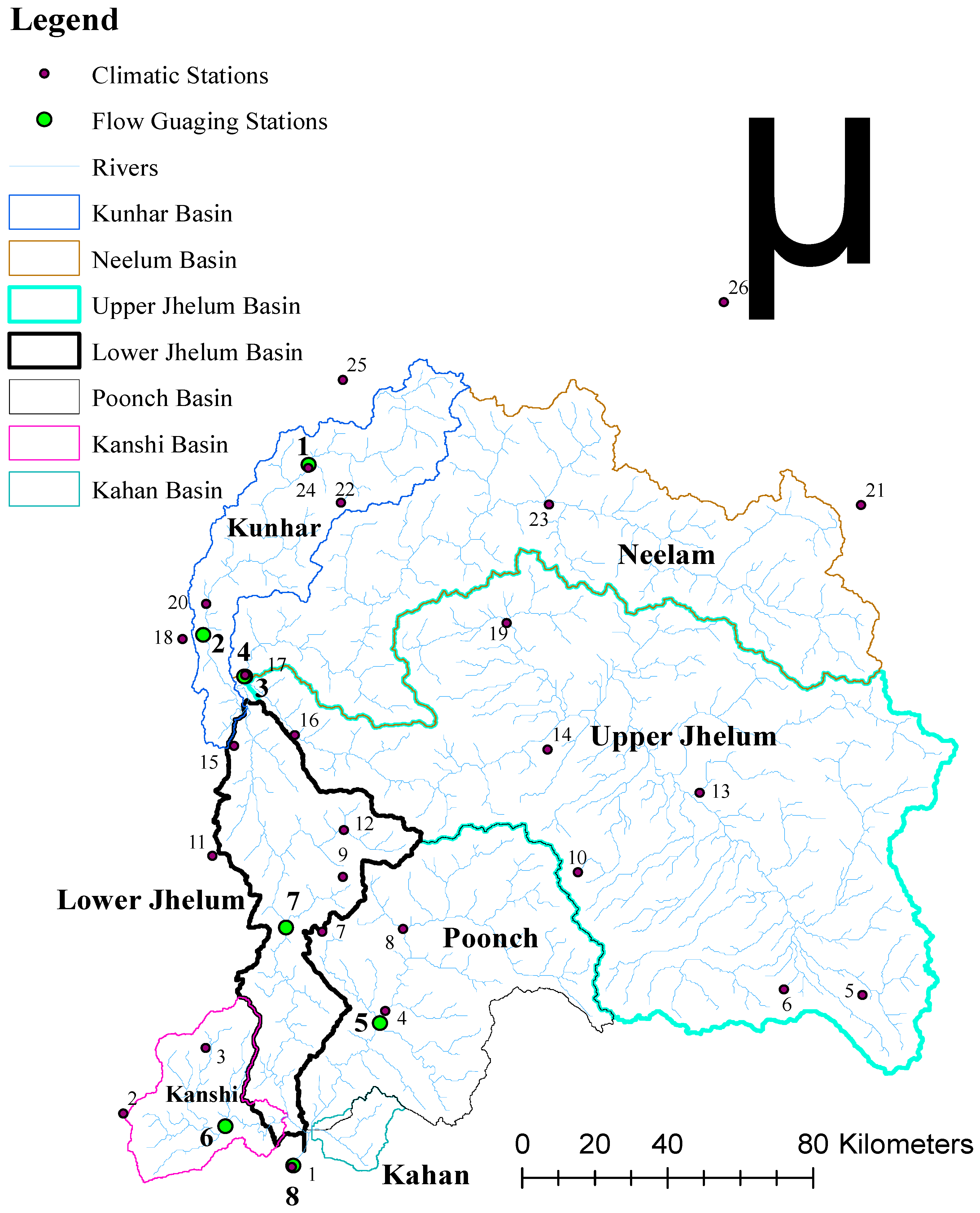
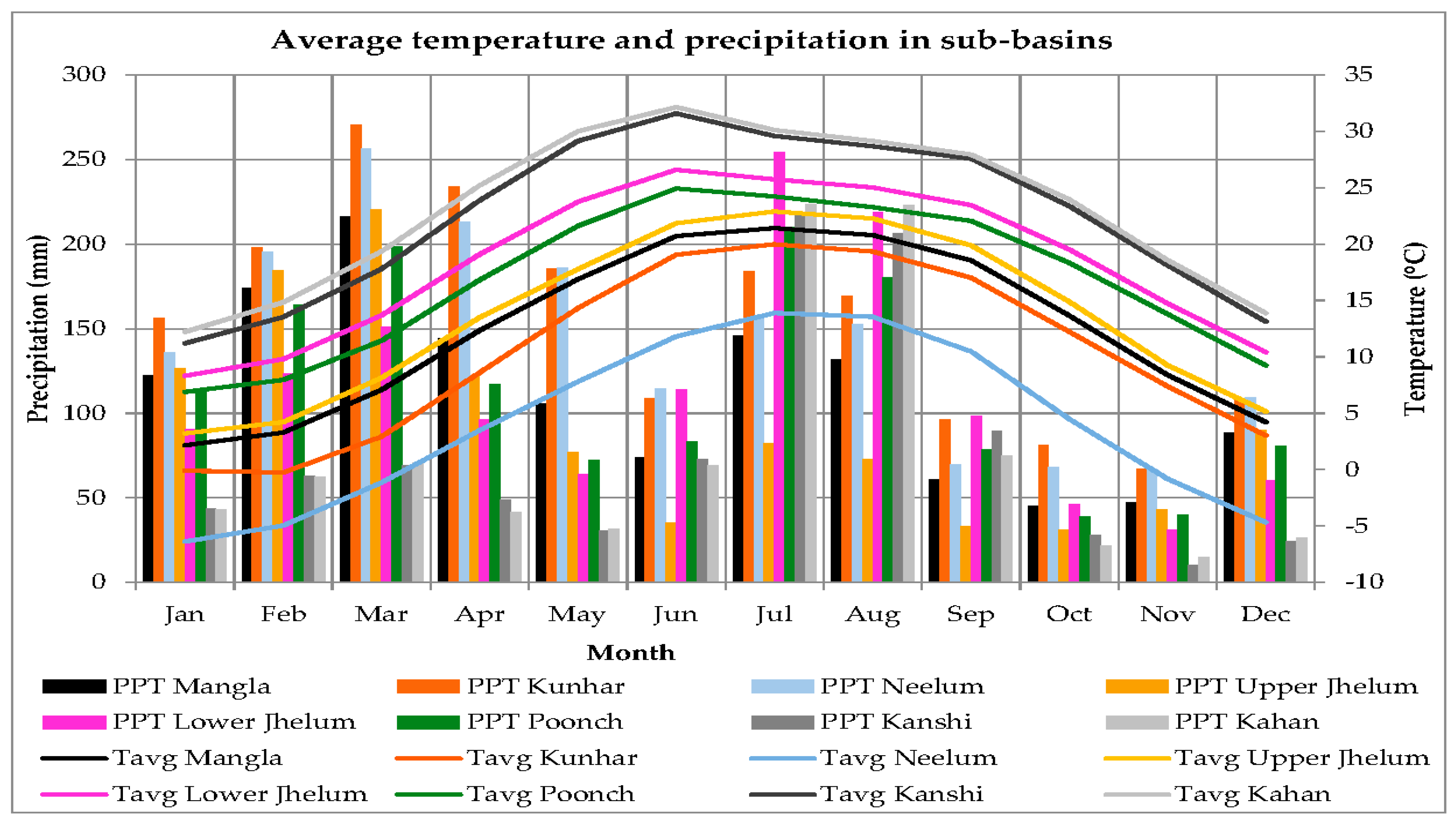
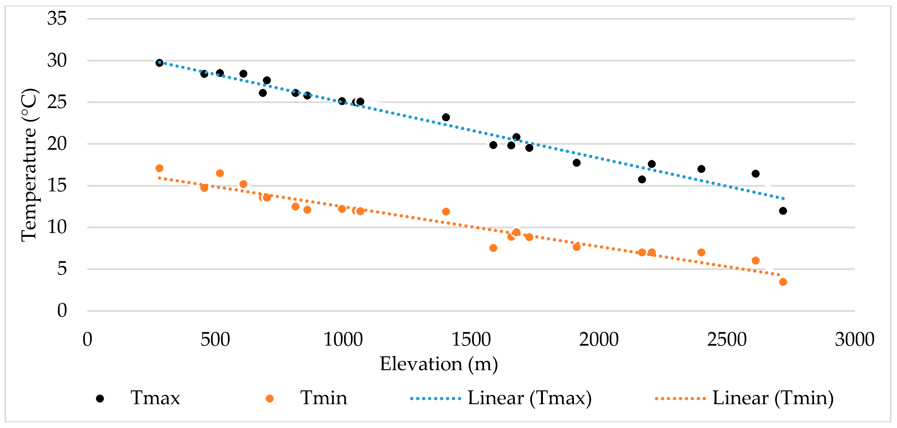
2. Study Area
3. Data
3.1. Observed Data
3.1.1. Meteorological Data
3.1.2. Discharge Data
3.1.3. Spatial Data
DEM
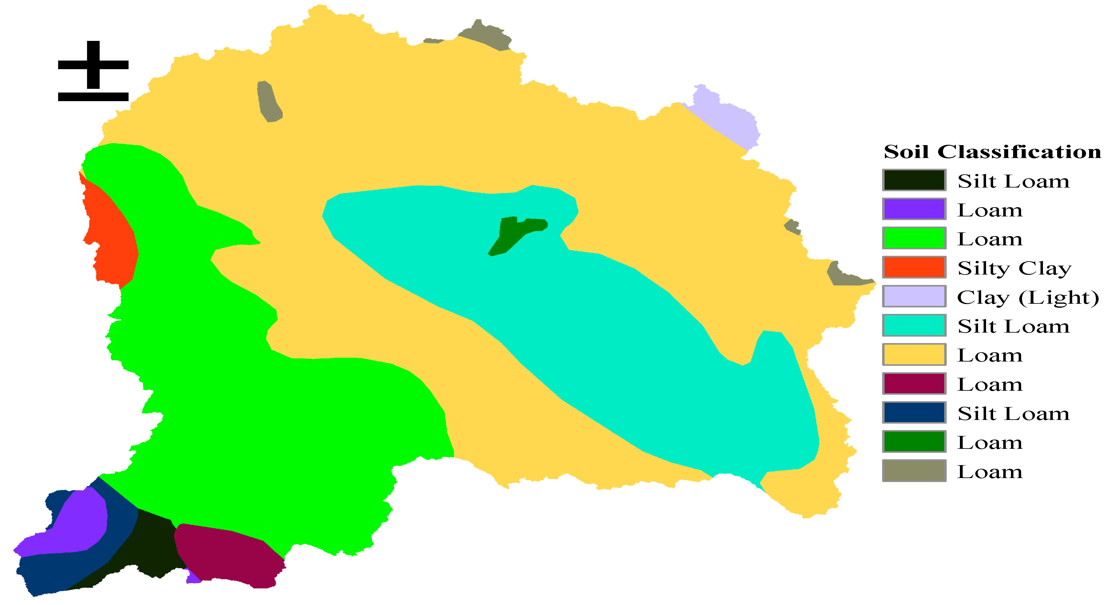
Soil Data
Landuse Data
3.2. Future Climate Data
4. Methodology
4.1. Selection of GCMs and Bias Correction
4.2. The SWAT Model Description
- The efficiency of the SWAT model is very high for the hydrological studies for the large catchment.
- Satisfactory simulation is obtained for daily, monthly, seasonally and annual runoffs.
- The performance of the snow-melting process of SWAT is satisfactory.
- Projection of streamflows under climate change is possible.
- SWAT is in the public domain.
- SW, soil water content
- t, time
- Ri, amount of precipitation
- Qi, amount of surface runoff
- ETi, amount of evapotranspiration
- Pi, amount of percolation
- QRi, amount of return flow
4.2.1. Model Calibration and Validation
4.2.2. Performance Evaluation
- Xi, measured value
- Xavg, average measured value
- Yi, simulated value
- Yavg, average simulated
4.3. Impact of Climate Change on Discharge
5. Results and Discussion
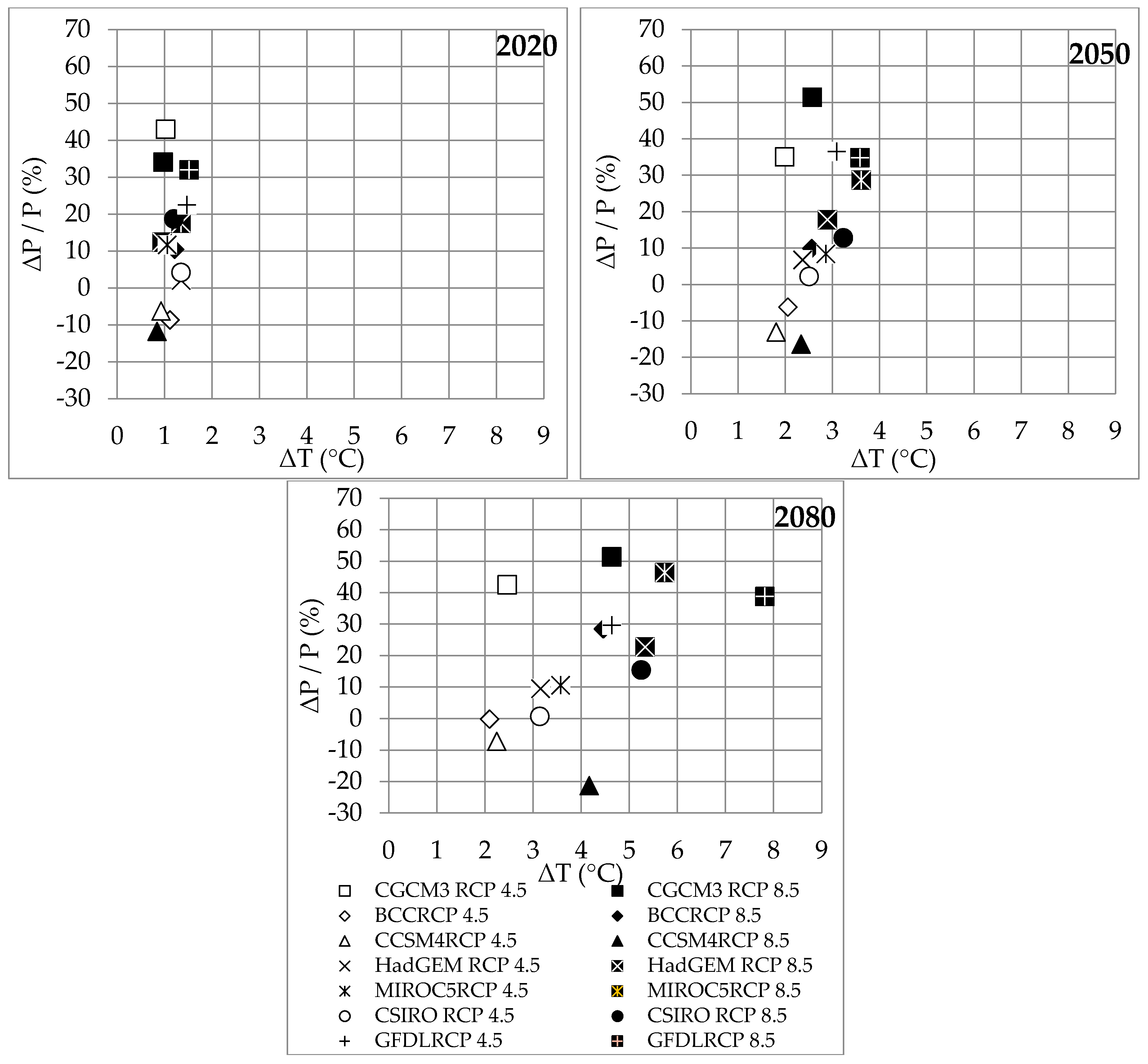
5.1. Climate Change
5.1.1. Annual
5.1.2. Seasonal
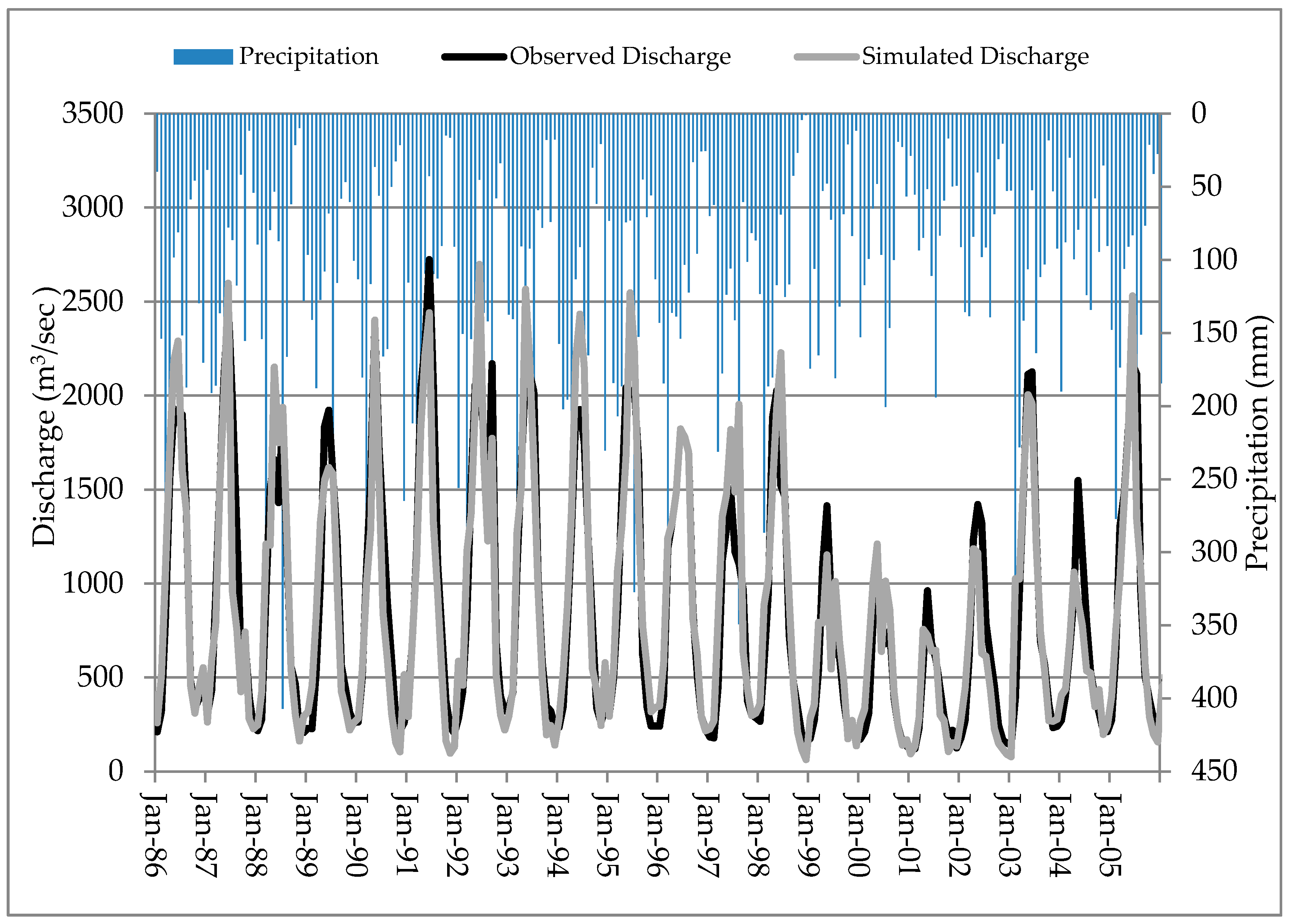
5.2. Model Calibration and Validation
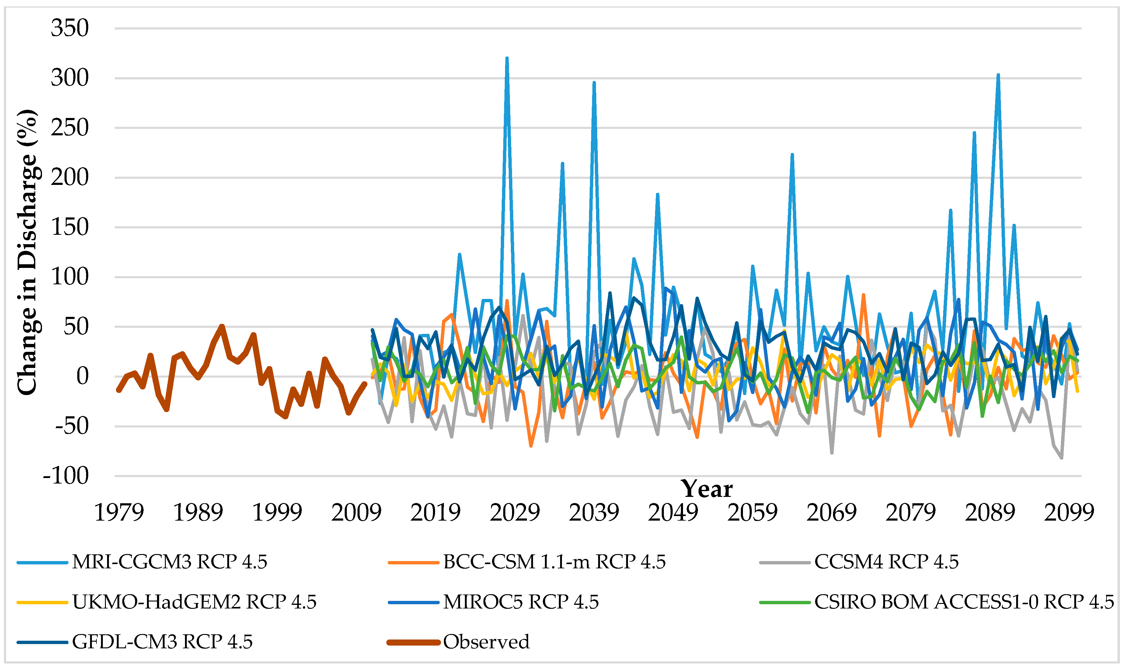
5.3. Impact of Climate Change on Discharge
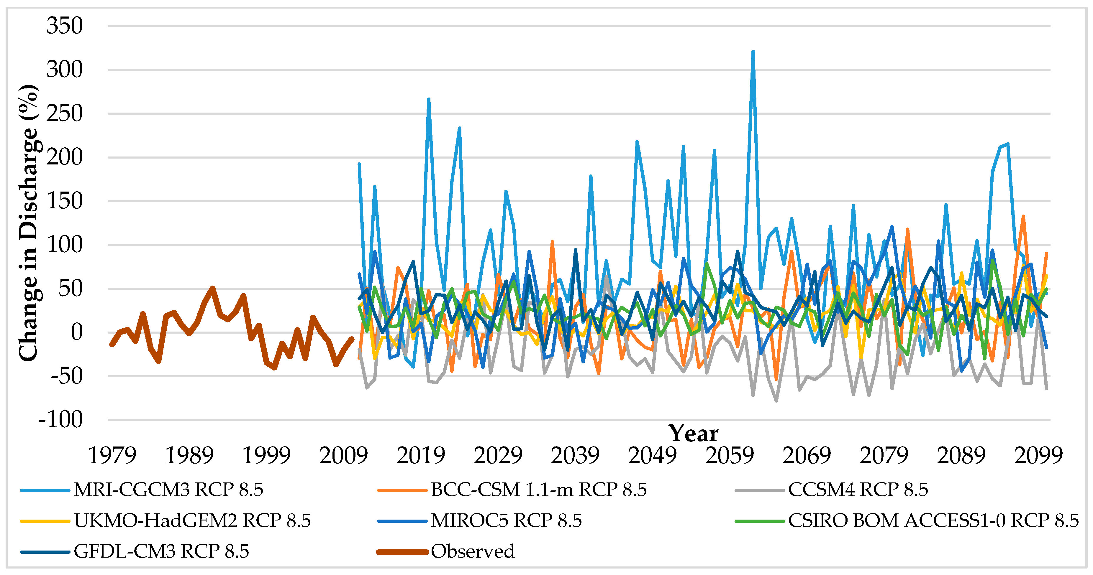
5.3.1. Annual and Seasonal Variations
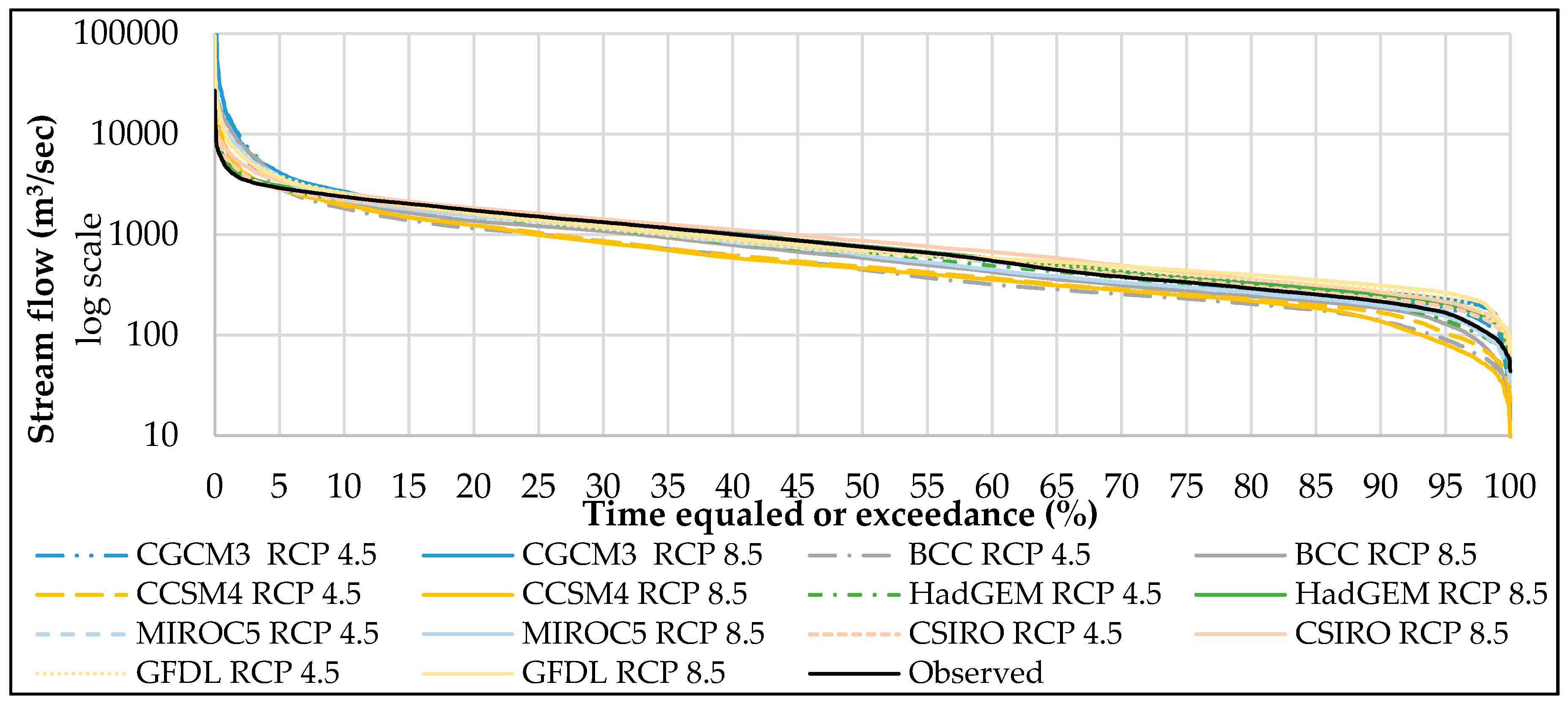
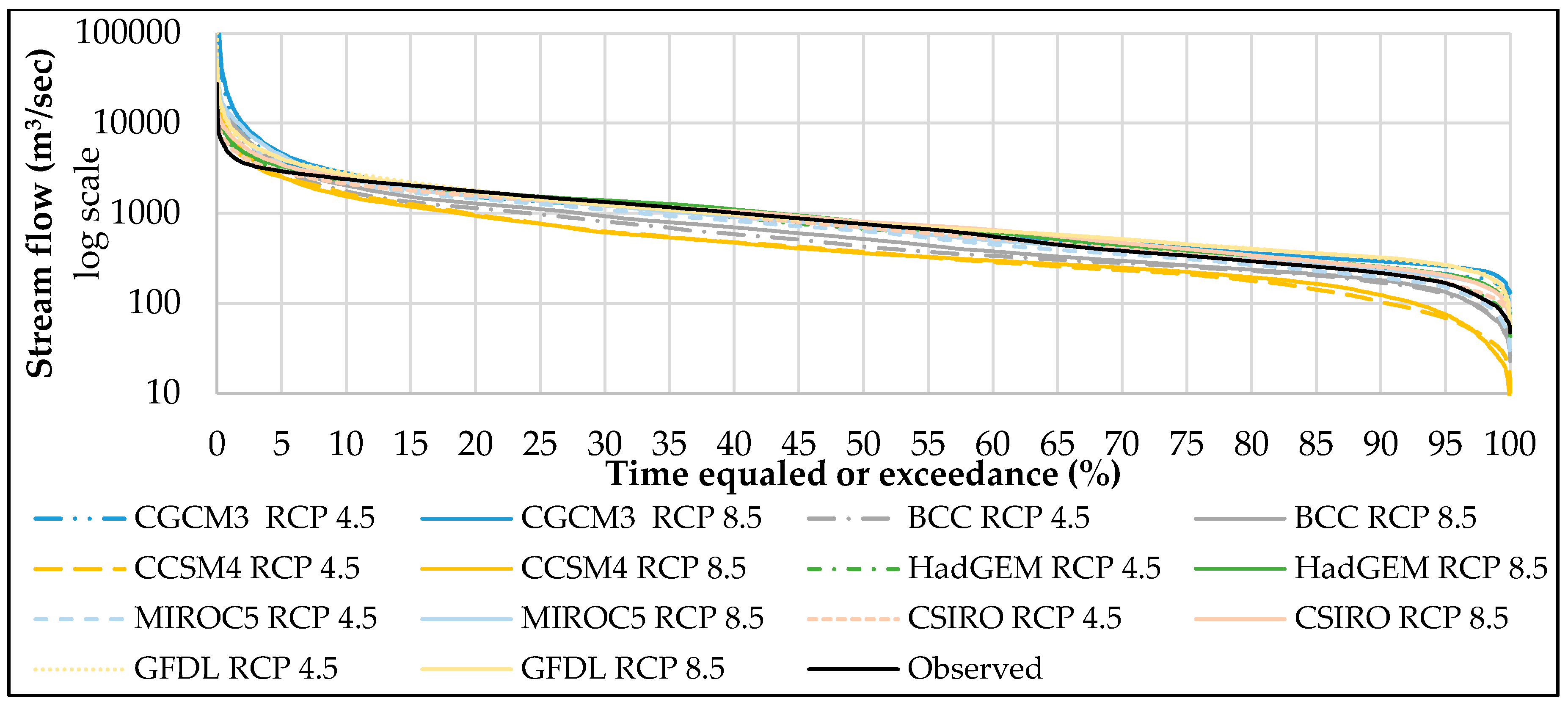
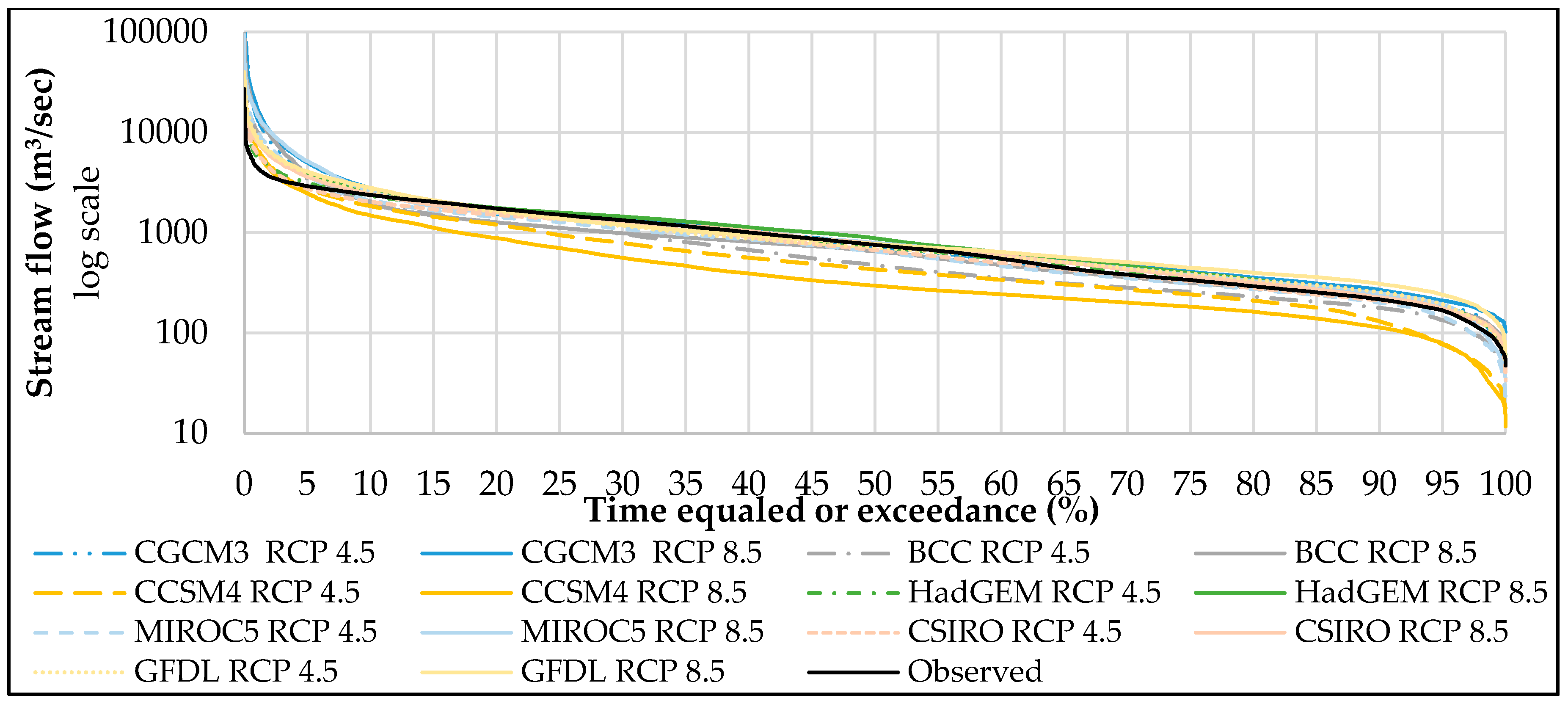
5.3.2. Changes in Flow Duration Curve as well as Low, Medium, and High Flows
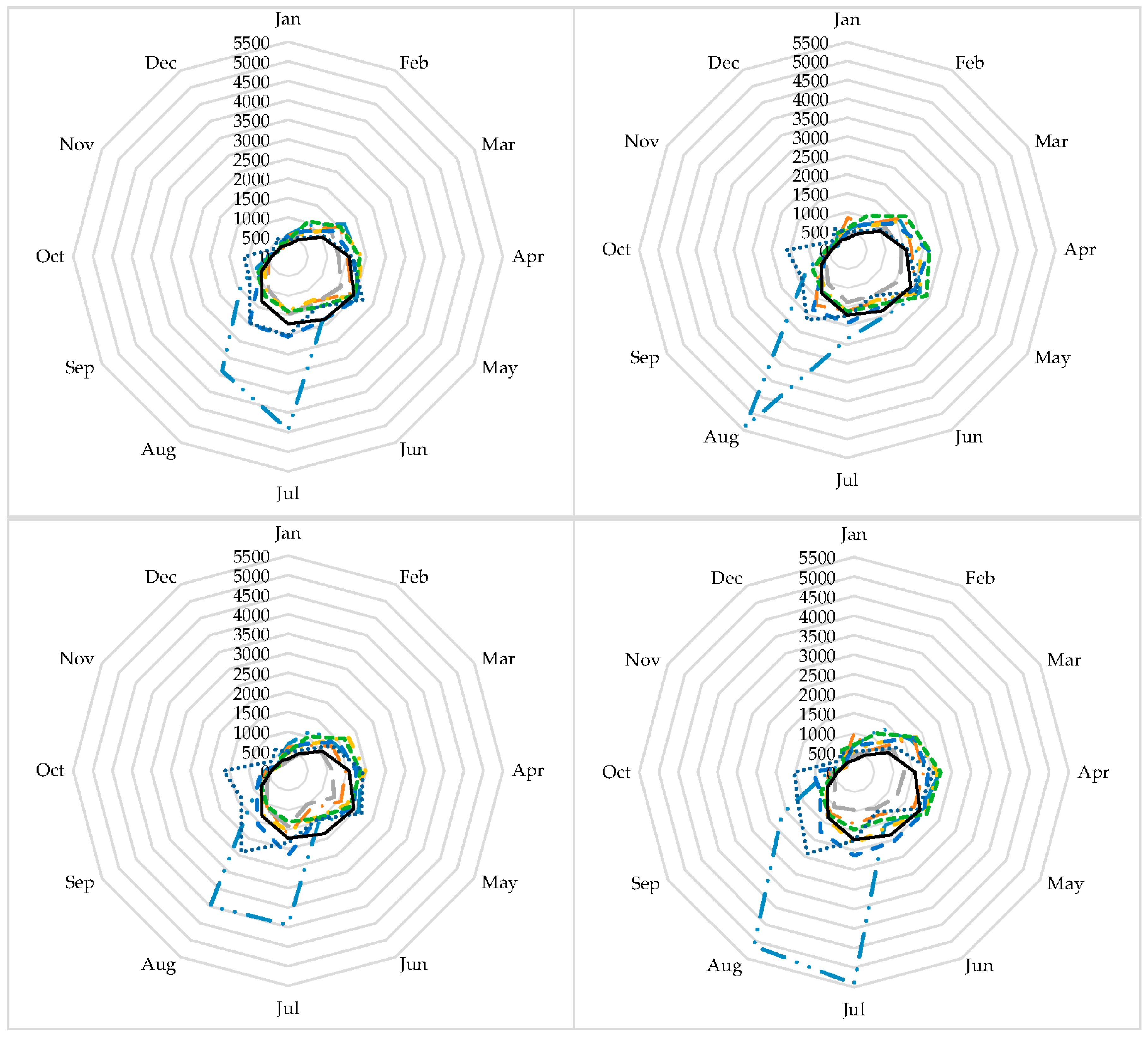
5.3.3. Temporal Shifts in Peak Flows
5.3.4. Temporal Shifts in Center-of-Volume Date (CVD)
6. Conclusions
- The Tmax and Tmin are projected to increase for all three-time horizons under both RCPs 4.5 and 8.5. The rise in Tmax is expected to be more than Tmin. Precipitation is projected to increase using five GCMs, while precipitation is projected to decrease using two GCMs under both RCPs 4.5 and 8.5.
- Mean annual flow was projected to increase in the basin under both RCP 4.5 and RCP 8.5 scenarios using six GCMs and expected to decrease using one GCM. An obvious increase in streamflow was predicted for winter and spring. However, summer and autumn showed a decrease in flow.
- High flows were predicted to increase but median flows were projected to decrease in the future under both scenarios. Flow duration curves showed that the probability of occurrence of high flow will be more in the future, relative to the baseline flows.
- Peaks were predicted to shift in the future. Similarly, center-of-volume date, a date at which half of the annual water passes, might change by about −11–23 days in the basin under both RCP 4.5 and RCP 8.5.
7. Limitations of the Study
Supplementary Materials
Acknowledgments
Author Contributions
Conflicts of Interest
Abbreviations
| °C | Degree Centigrade |
| ACCESS1-0 | Bureau of Meteorology, Australian Community Climate and Earth-System Simulator, Version 1.0 |
| AR5 | 5th Assessment Report |
| ARCGIS | Aeronautical Reconnaissance Coverage Geographic Information System |
| BCC-CSM | Beijing Climate Center, China Meteorological Administration |
| CCSM4 | Community Climate System Model Version 4 |
| CGCM3 | Canadian Centre for Climate Modeling Version 3 |
| CIMP5 | Climate Model Intercomparison Project Phase 5 |
| CSIRO BOM | Commonwealth Scientific and Industrial Research Organization |
| DEM | Digital Elevation Model |
| DJF | December, January, February |
| FAO | Food and Agricultural Organization |
| GCMs | General Circulation Models |
| GFDL-CM3 | Geophysical Fluid Dynamics Laboratory Climate Model Version 3 |
| GHGES | Greenhouse Gas Emission Scenarios |
| GIS | Geographical Information System |
| HEC-ResSim | Hydrologic Engineering Center Reservoir System Simulation |
| HPP | Hydropower Potential |
| HRU | Hydrologic Response Unit |
| IMD | Indian Metrological Department |
| IPCC | Intergovernmental Panel on Climate Change |
| JJA | June, July, August |
| km2 | Square Kilometers |
| km3 | Cubic Kilometers |
| LULC | Landuse Land Cover |
| m | Meter |
| m2 | Square Meters |
| m3 | Cubic Meters |
| MAM | March, April, May |
| MIROC5 | Model for Interdisciplinary Research on Climate Version 5 |
| mm | Millimeter |
| MODIS | Moderate Resolution Imaging Spectrometer |
| MRI-CGCM3 | Meteorological Research Institute Coupled General Circulation Model, Version 3 |
| MSL | Mean Sea Level |
| MW | Mega Watts |
| NSE | Nash-Sutcliffe Efficiency |
| PMD | Pakistan Metrological Department |
| RCP | Representative Concentration Pathway |
| SON | September, October, November |
| SRES | Special Report on Emission Scenarios |
| SRTM | Shuttle Radar Topography Mission |
| SUFI | Sequential Uncertainty Fitting |
| SWAT | Soil and Water Assessment Tool |
| SWAT-CUP | SWAT Calibration and Uncertainty Programs |
| SWHP | Surface Water Hydrology Project |
| UIB | Upper Indus Basin |
| UKMO-HadGEM | United Kingdom Meteorological Office, Hadley Centre of Global Environmental Model |
| UN | United Nations |
| USA | United States of America |
| USD | United States Dollar |
| USGS | United States Geological Survey |
| WAPDA | Water and Power Development Authority |
| WMO | World Meteorological Organization |
References
- Intergovernmental Panel on Climate Change (IPCC). The Scientific Basis; Cambridge University Press: Cambridge, UK; New York, NY, USA, 2001. [Google Scholar]
- Prasanna, V. Regional climate change scenarios over south asia in the cmip5 coupled climate model simulations. Meteorol. Atmos. Phys. 2015, 127, 561–578. [Google Scholar] [CrossRef]
- Zabaleta, A.; Meaurio, M.; Ruiz, E.; Antiguedad, I. Simulation climate change impact on runoff and sediment yield in a small watershed in the Basque Country, Northern Spain. J. Environ. Qual. 2014, 43, 235–245. [Google Scholar] [CrossRef] [PubMed]
- Velasco, P.P.; Bauwens, W. Climate change analysis of lake victoria outflows (Africa) using soil and water assessment tool (swat) and general circulation models (gcms). Asia Life Sci. 2013, 22, 659–675. [Google Scholar]
- Aronica, G.T.; Bonaccorso, B. Climate change effects on hydropower potential in the alcantara river basin in sicily (Italy). Earth Interact. 2013, 17. [Google Scholar] [CrossRef]
- Plangoen, P.; Babel, M.S.; Clemente, R.S.; Shrestha, S.; Tripathi, N.K. Simulating the impact of future land use and climate change on soil erosion and deposition in the mae nam nan sub-catchment, Thailand. Sustainability 2013, 5, 3244–3274. [Google Scholar] [CrossRef]
- Hormann, G.; Koplin, N.; Cai, Q.; Fohrer, N. Using a simple model as a tool to parameterise the swat model of the xiangxi river in China. Quat. Int. 2009, 208, 116–120. [Google Scholar] [CrossRef]
- Wang, B.; Lee, J.Y.; Xiang, B.Q. Asian summer monsoon rainfall predictability: A predictable mode analysis. Clim. Dyn. 2015, 44, 61–74. [Google Scholar] [CrossRef]
- Nicholls, R.J.; Marinova, N.; Lowe, J.A.; Brown, S.; Vellinga, P.; De Gusmao, D.; Hinkel, J.; Tol, R.S.J. Sea-level rise and its possible impacts given a ‘beyond 4 degrees c world’ in the twenty-first century. Philos. Trans. R. Soc. A 2011, 369, 161–181. [Google Scholar] [CrossRef] [PubMed]
- Dessai, S.; Hulme, M.; Lempert, R.; Pielke, R., Jr. Climate Prediction: A Limit to Adaptation; Cambridge University Press: New York, NY, USA, 2009; pp. 64–78. [Google Scholar]
- Mulligan, M. Climate change and food-water supply from africa’s drylands: Local impacts and teleconnections through global commodity flows. Int. J. Water Resour. D 2015, 31, 450–460. [Google Scholar] [CrossRef]
- Wanders, N.; van Lanen, H.A.J. Future discharge drought across climate regions around the world modelled with a synthetic hydrological modelling approach forced by three general circulation models. Nat. Hazards Earth Syst. Sci. 2015, 15, 487–504. [Google Scholar] [CrossRef]
- Babel, M.S.; Bhusal, S.P.; Wahid, S.M.; Agarwal, A. Climate change and water resources in the bagmati river basin, Nepal. Theor. Appl. Climatol. 2014, 115, 639–654. [Google Scholar] [CrossRef]
- Park, J.Y.; Park, M.J.; Ahn, S.R.; Park, G.A.; Yi, J.E.; Kim, G.S.; Srinivasan, R.; Kim, S.J. Assessment of future climate change impacts on water quantity and quality for a mountainous dam watershed using swat. Trans. ASABE 2011, 54, 1725–1737. [Google Scholar] [CrossRef]
- Booij, M.J.; Tollenaar, D.; van Beek, E.; Kwadijk, J.C.J. Simulating impacts of climate change on river discharges in the nile basin. Phys. Chem. Earth 2011, 36, 696–709. [Google Scholar] [CrossRef]
- Mahmood, R.; Babel, M.S.; Shaofeng, J.I.A. Assessment of temporal and spatial changes of future climate in the Jhelum river basin, Pakistan and India. Weather Clim. Extremes 2015, 10, 40–55. [Google Scholar] [CrossRef]
- Mahmood, R.; Babel, M.S. Evaluation of sdsm developed by annual and monthly sub-models for downscaling temperature and precipitation in the Jhelum Basin, Pakistan and India. Theor. Appl. Climatol. 2013, 113, 27–44. [Google Scholar] [CrossRef]
- Archer, D.R.; Fowler, H.J. Using meteorological data to forecast seasonal runoff on the river Jhelum, Pakistan. J. Hydrol. 2008, 361, 10–23. [Google Scholar] [CrossRef]
- Fowler, H.J.; Archer, D.R. Conflicting signals of climatic change in the upper indus basin. J. Clim. 2006, 19, 4276–4293. [Google Scholar] [CrossRef]
- Pervez, M.S.; Henebry, G.M. Projections of the ganges-brahmaputra precipitation downscaled from gcm predictors. J. Hydrol. 2014, 517, 120–134. [Google Scholar] [CrossRef]
- Reggiani, P.; Rientjes, T.H.M. A reflection on the long-term water balance of the upper indus basin. Hydrol. Res. 2015, 46, 446–462. [Google Scholar] [CrossRef]
- Sharma, V.; Mishra, V.D.; Joshi, P.K. Implications of climate change on streamflow of a snow-fed river system of the northwest himalaya. J. Mt. Sci. 2013, 10, 574–587. [Google Scholar] [CrossRef]
- Höök, M.; Sivertsson, A.; Aleklett, K. Validity of the fossil fuel production outlooks in the IPCC emission scenarios. Nat. Resour. Res. 2010, 19, 63–81. [Google Scholar] [CrossRef]
- Hawkins, E.; Sutton, R. The potential to narrow uncertainty in regional climate predictions. Bull. Am. Meteorol. Soc. 2009, 90, 1095–1107. [Google Scholar] [CrossRef]
- Majone, B.; Villa, F.; Deidda, R.; Bellin, A. Impact of climate change and water use policies on hydropower potential in the south-eastern alpine region. Sci. Total Environ. 2016, 543, 965–980. [Google Scholar] [CrossRef] [PubMed]
- Mall, R.K.; Gupta, A.; Singh, R.; Singh, R.S.; Rathore, L.S. Water resources and climate change: An Indian perspective. Curr. Sci. 2006, 90, 1610–1626. [Google Scholar]
- Mahmood, R.; Jia, S.; Babel, M.S. Potential impacts of climate change on water resources in the kunhar river basin, Pakistan. Water 2016, 8, 23. [Google Scholar] [CrossRef]
- Sarwar, S. Reservoir Life Expectancy in Relation to Climate and Land-Use Changes: Case Study of the Mangla Reservoir in Pakistan; University of Waikato: Hamilton, New Zealand, 2013. [Google Scholar]
- Yaseen, M.; Nabi, G.; Latif, M. Assessment of climate change at spatiao-temporal scales and its impact on stream flows in mangla watershed. Pak. J. Eng. Appl. Sci. 2016, 15, 17–39. [Google Scholar]
- Akhtar, M.; Ahmad, N.; Booij, M.J. The impact of climate change on the water resources of hindukush-karakorum-himalaya region under different glacier coverage scenarios. J. Hydrol. 2008, 355, 148–163. [Google Scholar] [CrossRef]
- Arnell, N.W. Effects of ipccsres emissions scenarios on river runoff: A global perspective. Hydrol. Earth Syst. Sci. 2003, 7, 619–641. [Google Scholar] [CrossRef]
- Food and Agriculture Organization (FAO). Digital Soil Map of the World and Derived Soil Properties; Version 3.5; FAO: Rome, Italy, 1995. [Google Scholar]
- Dile, Y.T.; Srinivasan, R. Evaluation of cfsr climate data for hydrologic prediction in data-scarce watersheds: An application in the blue nile river basin. J. Am. Water Resour. Assoc. 2014, 50, 1226–1241. [Google Scholar] [CrossRef]
- Fuka, D.R.; Walter, M.T.; MacAlister, C.; Degaetano, A.T.; Steenhuis, T.S.; Easton, Z.M. Using the climate forecast system reanalysis as weather input data for watershed models. Hydrol. Process. 2014, 28, 5613–5623. [Google Scholar] [CrossRef]
- Su, B.D.; Zeng, X.F.; Zhai, J.Q.; Wang, Y.J.; Li, X.C. Projected precipitation and streamflow under sres and rcp emission scenarios in the songhuajiang river basin, China. Quat. Int. 2015, 380, 95–105. [Google Scholar] [CrossRef]
- Hulme, M. Climate Change and Southern Africa: An Exploration of Some Potential Impacts and Implications for the Sadc Region; Climatic Research Unit, University of East Anglia: Norwich, UK, 1996. [Google Scholar]
- San Jose, R.; Perez, J.L.; Gonzalez, R.M.; Pecci, J.; Garzon, A.; Palacios, M. Impacts of the 4.5 and 8.5 rcp global climate scenarios on urban meteorology and air quality: Application to Madrid, Antwerp, Milan, Helsinki and London. J. Comput. Appl. Math. 2016, 293, 192–207. [Google Scholar] [CrossRef]
- Hu, Y.R.; Maskey, S.; Uhlenbrook, S. Downscaling daily precipitation over the yellow river source region in China: A comparison of three statistical downscaling methods. Theor. Appl. Climatol. 2013, 112, 447–460. [Google Scholar] [CrossRef]
- Fang, G.H.; Yang, J.; Chen, Y.N.; Zammit, C. Comparing bias correction methods in downscaling meteorological variables for a hydrologic impact study in an arid area in China. Hydrol. Earth Syst. Sci. 2015, 19, 2547–2559. [Google Scholar] [CrossRef] [Green Version]
- Ouyang, F.; Zhu, Y.H.; Fu, G.B.; Lu, H.S.; Zhang, A.J.; Yu, Z.B.; Chen, X. Impacts of climate change under cmip5 rcp scenarios on streamflow in the huangnizhuang catchment. Stoch. Environ. Res. Risk Assess. 2015, 29, 1781–1795. [Google Scholar] [CrossRef]
- Ma, C.K.; Sun, L.; Liu, S.Y.; Shao, M.A.; Luo, Y. Impact of climate change on the streamflow in the glacierized chu river basin, central asia. J. Arid Land 2015, 7, 501–513. [Google Scholar] [CrossRef]
- Bannwarth, M.A.; Hugenschmidt, C.; Sangchan, W.; Lamers, M.; Ingwersen, J.; Ziegler, A.D.; Streck, T. Simulation of stream flow components in a mountainous catchment in northern thailand with swat, using the anselm calibration approach. Hydrol. Process. 2015, 29, 1340–1352. [Google Scholar] [CrossRef]
- Memarian, H.; Balasundram, S.K.; Abbaspour, K.C.; Talib, J.B.; Sung, C.T.B.; Sood, A.M. Swat-based hydrological modelling of tropical land-use scenarios. Hydrol. Sci. J. 2014, 59, 1808–1829. [Google Scholar] [CrossRef]
- Saha, P.P.; Zeleke, K.; Hafeez, M. Streamflow modeling in a fluctuant climate using swat: Yass river catchment in South Eastern Australia. Environ. Earth Sci. 2014, 71, 5241–5254. [Google Scholar] [CrossRef]
- Chiang, L.C.; Yuan, Y.P.; Mehaffey, M.; Jackson, M.; Chaubey, I. Assessing swat’s performance in the kaskaskia river watershed as influenced by the number of calibration stations used. Hydrol. Process. 2014, 28, 676–687. [Google Scholar] [CrossRef]
- Arnold, J.G.; Srinivasan, R.; Muttiah, R.S.; Williams, J.R. Large area hydrologic modeling and assessment part I: Model development1. J. Am. Water Resour. Assoc. 1998, 34, 73–89. [Google Scholar] [CrossRef]
- Haguma, D.; Leconte, R.; Cote, P.; Krau, S.; Brissette, F. Optimal hydropower generation under climate change conditions for a northern water resources system. Water Resour. Manag. 2014, 28, 4631–4644. [Google Scholar] [CrossRef]
- Park, J.Y.; Kim, S.J. Potential impacts of climate change on the reliability of water and hydropower supply from a multipurpose dam in South Korea. J. Am. Water Resour Assoc. 2014, 50, 1273–1288. [Google Scholar] [CrossRef]
- Rahman, K.; Maringanti, C.; Beniston, M.; Widmer, F.; Abbaspour, K.; Lehmann, A. Streamflow modeling in a highly managed mountainous glacier watershed using swat: The upper rhone river watershed case in Switzerland. Water Resour. Manag. 2013, 27, 323–339. [Google Scholar] [CrossRef]
- Ahmad, Z.; Hafeez, M.; Ahmad, I. Hydrology of mountainous areas in the upper indus basin, northern pakistan with the perspective of climate change. Environ. Monit. Assess. 2012, 184, 5255–5274. [Google Scholar] [CrossRef] [PubMed]
- Butts, M.B.; Payne, J.T.; Kristensen, M.; Madsen, H. An evaluation of the impact of model structure on hydrological modelling uncertainty for streamflow simulation. J. Hydrol. 2004, 298, 242–266. [Google Scholar] [CrossRef]
- Krause, P.; Boyle, D.; Bäse, F. Comparison of different efficiency criteria for hydrological model assessment. Adv. Geosci. 2005, 5, 89–97. [Google Scholar] [CrossRef]
- Srinivasan, R.; Zhang, X.; Arnold, J. Swat ungauged: Hydrological budget and crop yield predictions in the upper mississippi river basin. Trans. ASABE 2010, 53, 1533–1546. [Google Scholar] [CrossRef]
- Klipsch, J.; Hurst, M. HEC-Ressim Reservoir System Simulation User’s Manual Version 3.0; USACE: Davis, CA, USA, 2007; p. 512. [Google Scholar]
- Teshager, A.D.; Gassman, P.W.; Secchi, S.; Schoof, J.T.; Misgna, G. Modeling agricultural watersheds with the soil and water assessment tool (swat): Calibration and validation with a novel procedure for spatially explicit hrus. Environ. Manag. 2016, 57, 894–911. [Google Scholar] [CrossRef] [PubMed]
- Singh, D.; Gupta, R.D.; Jain, S.K. Assessment of impact of climate change on water resources in a hilly river basin. Arab. J. Geosci. 2015, 8, 10625–10646. [Google Scholar] [CrossRef]
- Ligaray, M.; Kim, H.; Sthiannopkao, S.; Lee, S.; Cho, K.H.; Kim, J.H. Assessment on hydrologic response by climate change in the chao phraya river basin, Thailand. Water 2015, 7, 6892–6909. [Google Scholar] [CrossRef]
- Deb, D.; Butcher, J.; Srinivasan, R. Projected hydrologic changes under mid-21st century climatic conditions in a sub-arctic watershed. Water Resour. Manag. 2015, 29, 1467–1487. [Google Scholar] [CrossRef]
- Neitsch, S.; Arnold, J.; Kiniry, J.E.A.; Srinivasan, R.; Williams, J. Soil and Water Assessment Tool User’s Manual Version 2000; GSWRL Report; Texas Water Resources Institute: College Station, TX, USA, 2002; p. 202. [Google Scholar]


| No. | Name | Latitude N | Longitude E | Elevation M, MSL | Data Source | Data Availability |
|---|---|---|---|---|---|---|
| 1 | Mangla | 33.12 | 73.63 | 282 | PMD | 1960–2010 |
| 2 | Gujjar Khan | 33.25 | 73.13 | 547 | PMD | 1960–2010 |
| 3 | Kallar | 33.42 | 73.37 | 518 | PMD | 1960–2010 |
| 4 | Rehman Br.(Kotli) | 33.52 | 73.9 | 614 | PMD | 1960–2010 |
| 5 | 33.565 | 75.313 | 2317 | CFSR data | 1979–2010 | |
| 6 | 33.58 | 75.08 | 1690 | CFSR data | 1979–2010 | |
| 7 | Palandri | 33.72 | 73.71 | 1402 | SWHP | 1962–2010 |
| 8 | Sehr kakota | 33.73 | 73.95 | 915 | PMD | 1961–2010 |
| 9 | Rawalakot | 33.86 | 73.77 | 1676 | SWHP | 1960–2010 |
| 10 | 33.877 | 74.468 | 2154 | CFSR data | 1979–2010 | |
| 11 | Murree | 33.91 | 73.38 | 2213 | SWHP | 1960–2010 |
| 12 | Bagh | 33.98 | 73.77 | 1067 | SWHP | 1961–2010 |
| 13 | Srinagar | 34.08 | 74.83 | 1587 | IMD | 1892–2010 |
| 14 | 34.189 | 74.375 | 1821 | CFSR data | 1979–2010 | |
| 15 | Domel | 34.19 | 73.44 | 702 | SWHP | 1961–2010 |
| 16 | Gharidopatta | 34.22 | 73.62 | 814 | PMD | 1954–2010 |
| 17 | Muzaffarabad | 34.37 | 73.47 | 686 | SWHP | 1962–2010 |
| 18 | Shinkiari | 34.46 | 73.28 | 1050 | PMD | 1961–2010 |
| 19 | Kupwara | 34.51 | 74.25 | 1609 | IMD | 1960–2010 |
| 20 | Balakot | 34.55 | 73.35 | 995.4 | PMD | 1961–2010 |
| 21 | 34.813 | 75.313 | 4360 | CFSR data | 1979–2010 | |
| 22 | 34.813 | 73.75 | 3720 | CFSR data | 1979–2010 | |
| 23 | 34.813 | 74.375 | 2612 | CFSR data | 1979–2010 | |
| 24 | Naran | 34.9 | 73.65 | 2362 | PMD | 1961–2010 |
| 25 | 35.126 | 73.75 | 3284 | CFSR data | 1979–2010 | |
| 26 | Astore | 35.33 | 74.9 | 2168 | PMD | 1954–2010 |
| No. | Station | River | Latitude | Longitude | Elevation | Area | Observation Period |
|---|---|---|---|---|---|---|---|
| N | E | M, MSL | km2 | ||||
| 1 | Naran | Kunhar | 34.908 | 73.651 | 2400 | 1036 | 1960–2010 |
| 2 | Garhi Habib Ullah/Talhatta | Kunhar | 34.472 | 73.342 | 900 | 2354 | 1960–2010 |
| 3 | Muzaffar Abad | Neelum | 34.367 | 73.469 | 670 | 7278 | 1962–2010 |
| 4 | Domel | Jhelum | 34.367 | 73.467 | 701 | 14,504 | 1974–2010 |
| 5 | Kotli | Poonch | 33.489 | 73.885 | 530 | 3238 | 1960–2010 |
| 6 | Palote | Kanshi | 33.222 | 73.432 | 400 | 1111 | 1970–2010 |
| 7 | Azad Pattan | Jhelum | 33.73 | 73.603 | 485 | 26,485 | 1974–2010 |
| 8 | Mangla | Jhelum | 33.124 | 73.633 | 282 | 33,470 | 1922–2010 |
| Station Name | Jan. | Feb. | Mar. | Apr. | May | Jun. | Jul. | Aug. | Sep. | Oct. | Nov. | Dec. | Annual (J–D) |
|---|---|---|---|---|---|---|---|---|---|---|---|---|---|
| Naran | 10 | 8 | 8 | 21 | 76 | 142 | 124 | 68 | 35 | 21 | 15 | 12 | 45 |
| Garihabib | 24 | 26 | 46 | 100 | 196 | 258 | 230 | 144 | 81 | 46 | 32 | 28 | 101 |
| Muzafffar Abad | 64 | 79 | 179 | 472 | 780 | 798 | 630 | 414 | 227 | 115 | 83 | 67 | 326 |
| Domel | 105 | 183 | 411 | 616 | 681 | 519 | 446 | 367 | 250 | 136 | 99 | 101 | 326 |
| Kotli | 58 | 103 | 189 | 178 | 127 | 119 | 225 | 255 | 136 | 101 | 45 | 57 | 133 |
| Polatoe | 2 | 4 | 3 | 3 | 1 | 2 | 20 | 21 | 8 | 2 | 1 | 2 | 6 |
| Azad Pattan | 231 | 360 | 749 | 1317 | 1763 | 1676 | 1415 | 1025 | 629 | 349 | 249 | 234 | 833 |
| Mangla | 308 | 498 | 998 | 1551 | 1929 | 1833 | 1728 | 1378 | 813 | 482 | 309 | 309 | 1011 |
| Soil Type | Percentage of Basin Area (%) | Texture | Soil Bulk Density (g/cm3) | Hydrologic Group | Soil Available Water Capacity (mm/mm) | Hydraulic Conductivity (mm/h) | Composition (%) | Soil Electric Conductivity (ds/m) | ||
|---|---|---|---|---|---|---|---|---|---|---|
| Sand | Silt | Clay | ||||||||
| Gelic Regosols | 1.1 | Silt loam | 1.47 | B | 150 | 0.02 | 26 | 63 | 11 | 0.1 |
| Gleyic Solonetz | 1.1 | Loam | 1.36 | B | 150 | 0.02 | 32 | 43 | 25 | 1.6 |
| Calcaric Phaeozems | 22.9 | Loam | 1.38 | B | 150 | 0.02 | 35 | 43 | 22 | 0.2 |
| Calcic Chernozems | 1.1 | Silty clay | 1.24 | B | 150 | 0.01 | 13 | 42 | 45 | 0.2 |
| Luvic Chernozems | 0.7 | Clay (light) | 1.25 | C | 150 | 0.05 | 19 | 37 | 44 | 0.5 |
| Mollic Planosols | 20.2 | Silt loam | 1.35 | B | 150 | 0.02 | 24 | 52 | 24 | 0.1 |
| Gleyic Solonchaks | 48.6 | Loam | 1.39 | C | 150 | 0.07 | 37 | 42 | 21 | 8.7 |
| Haplic Solonetz | 1.5 | Loam | 1.39 | B | 150 | 0.02 | 47 | 29 | 24 | 0.1 |
| Haplic Chernozems | 1.6 | Silt loam | 1.35 | B | 150 | 0.02 | 23 | 54 | 23 | 0.1 |
| Dystric Cambisols | 0.4 | Loam | 1.41 | B | 100 | 0.02 | 42 | 38 | 20 | 0.1 |
| Lithic Leptosols | 0.7 | Loam | 1.38 | B | 150 | 0.02 | 42 | 34 | 24 | 0.1 |
| Model | Name | Country | Spatial Resolution |
|---|---|---|---|
| BCC-CSM 1.1-m | Beijing Climate Center (BCC), China Meteorological Administration Model | China | 1.9° × 1.9° |
| CCSM4 | Community Climate System Model (CCSM) National Center for Atmospheric Research (NCAR) | USA | 0.94° × 1.25° |
| CSIRO BOM ACCESS1-0 | Commonwealth Scientific and Industrial Research Organization, Bureau of Meteorology, Australian Community Climate and Earth-System Simulator, version 1.0 | Australia | 1.9° × 1.9° |
| GFDL-CM3 | Geophysical Fluid Dynamics Laboratory Climate Model, version 3 | USA | 2.5° × 2.0° |
| MIROC5 | Model for Interdisciplinary Research on Climate version 5 | Japan | 1.41° × 1.41° |
| MRI-CGCM3 | Meteorological Research Institute Coupled General Circulation Model, version 3 | Canada | 1.9° × 1.9° |
| UKMO-HadGEM2 | United Kingdom Meteorological Office Hadley Centre Global Environmental Model version 2 | UK | 2.80° × 2.80° |
| No. | GCM | Period | RCP | Average Increase Tmax (°C) | Average Increase Tmin (°C) | Change in PPT (%) | ||||||||||||
|---|---|---|---|---|---|---|---|---|---|---|---|---|---|---|---|---|---|---|
| DJF | MAM | JJA | SON | Annual | DJF | MAM | JJA | SON | Annual | DJF | MAM | JJA | SON | Annual | ||||
| 1 | MRI-CGCM3 | 2020s | 4.5 | 0.7 | 0.6 | 0.5 | 0.2 | 0.5 | 2.0 | 1.6 | 1.3 | 1.3 | 1.5 | 7.3 | 13.3 | 95.2 | 69.6 | 43.0 |
| 2 | BCC-CSM 1.1-m | 2020s | 4.5 | 1.6 | 0.9 | 1.2 | 1.2 | 1.2 | 1.4 | 0.7 | 0.8 | 1.1 | 1.0 | −13.7 | −1.3 | −11.1 | −10.5 | −8.7 |
| 3 | CCSM4 | 2020s | 4.5 | 0.9 | 1.5 | 0.6 | 0.9 | 0.9 | 0.7 | 1.2 | 0.9 | 0.9 | 0.9 | −10.1 | −17.3 | 1.2 | 13.0 | −6.2 |
| 4 | UKMO-HadGEM | 2020s | 4.5 | 2.1 | 1.5 | 0.9 | 1.5 | 1.5 | 1.5 | 1.6 | 0.9 | 0.8 | 1.2 | −33.4 | 48.1 | −18.3 | 12.5 | 2.1 |
| 5 | MIROC5 | 2020s | 4.5 | 0.4 | 1.4 | 0.9 | 1.1 | 1.0 | 0.6 | 1.5 | 1.5 | 1.1 | 1.1 | 2.2 | −5.9 | 49.8 | −18.2 | 11.7 |
| 6 | CSIRO BOM | 2020s | 4.5 | 1.8 | 1.3 | 0.5 | 1.3 | 1.2 | 2.0 | 1.5 | 1.1 | 1.3 | 1.5 | 7.1 | 11.4 | 3.0 | −18.2 | 4.2 |
| 7 | GFDL-CM3 | 2020s | 4.5 | 1.8 | 1.5 | 1.3 | 1.8 | 1.6 | 1.2 | 1.1 | 1.5 | 1.5 | 1.3 | −18.5 | −2.6 | 43.9 | 128.4 | 22.5 |
| 8 | MRI-CGCM3 | 2020s | 8.5 | 0.6 | 0.4 | 0.5 | 0.0 | 0.4 | 2.0 | 1.4 | 1.4 | 1.4 | 1.6 | −4.9 | 10.4 | 91.7 | 37.9 | 34.1 |
| 9 | BCC-CSM 1.1-m | 2020s | 8.5 | 1.5 | 1.4 | 1.0 | 1.4 | 1.3 | 1.6 | 1.0 | 0.7 | 1.2 | 1.1 | 10.5 | 2.7 | 10.3 | 31.8 | 10.5 |
| 10 | CCSM4 | 2020s | 8.5 | 1.2 | 1.4 | 0.9 | 0.9 | 1.1 | 0.5 | 0.9 | 0.6 | 0.4 | 0.6 | −29.7 | −0.9 | −1.7 | −25.7 | −11.7 |
| 11 | UKMO-HadGEM | 2020s | 8.5 | 1.1 | 0.7 | 0.5 | 0.8 | 0.8 | 1.2 | 1.2 | 0.9 | 1.2 | 1.1 | −23.5 | 63.4 | −12.0 | 21.4 | 12.5 |
| 12 | MIROC5 | 2020s | 8.5 | 0.7 | 1.4 | 1.3 | 1.0 | 1.1 | 1.2 | 1.9 | 1.9 | 1.4 | 1.6 | 14.0 | 5.4 | 18.8 | 54.9 | 17.5 |
| 13 | CSIRO BOM | 2020s | 8.5 | 1.1 | 1.4 | 0.5 | 1.4 | 1.1 | 1.2 | 1.6 | 1.0 | 1.3 | 1.3 | 29.0 | 27.7 | 5.4 | 5.8 | 18.8 |
| 14 | GFDL-CM3 | 2020s | 8.5 | 2.1 | 1.3 | 1.2 | 1.4 | 1.5 | 1.9 | 1.1 | 1.8 | 1.4 | 1.5 | −6.7 | −4.9 | 47.0 | 180.3 | 32.0 |
| 15 | MRI-CGCM3 | 2050s | 4.5 | 1.3 | 2.1 | 1.7 | 1.0 | 1.5 | 2.9 | 2.6 | 2.2 | 2.2 | 2.5 | 23.5 | −14.7 | 85.2 | 65.7 | 35.1 |
| 16 | BCC-CSM 1.1-m | 2050s | 4.5 | 3.0 | 3.1 | 1.6 | 1.6 | 2.3 | 2.5 | 2.2 | 1.1 | 1.4 | 1.8 | −11.2 | −18.3 | 2.8 | 14.5 | −6.2 |
| 17 | CCSM4 | 2050s | 4.5 | 2.2 | 2.4 | 1.5 | 1.7 | 2.0 | 1.5 | 2.0 | 1.5 | 1.6 | 1.6 | −45.1 | −23.5 | 13.9 | 19.0 | −13.0 |
| 18 | UKMO-HadGEM | 2050s | 4.5 | 3.1 | 2.7 | 1.3 | 3.0 | 2.5 | 2.6 | 2.5 | 2.0 | 1.7 | 2.2 | −21.2 | 47.1 | −1.9 | −14.9 | 6.8 |
| 19 | MIROC5 | 2050s | 4.5 | 2.6 | 4.0 | 3.1 | 2.2 | 3.0 | 2.5 | 3.4 | 3.2 | 1.8 | 2.7 | −4.6 | −14.0 | 45.8 | 1.5 | 8.4 |
| 20 | CSIRO BOM | 2050s | 4.5 | 2.8 | 2.8 | 1.7 | 2.6 | 2.5 | 3.1 | 2.7 | 2.0 | 2.1 | 2.5 | 8.2 | 7.2 | 3.6 | −28.0 | 2.2 |
| 21 | GFDL-CM3 | 2050s | 4.5 | 3.1 | 3.1 | 2.8 | 3.8 | 3.2 | 2.5 | 2.6 | 3.2 | 3.6 | 3.0 | −6.0 | −3.3 | 60.1 | 178.9 | 36.5 |
| 22 | MRI-CGCM3 | 2050s | 8.5 | 1.9 | 2.2 | 2.1 | 1.4 | 1.9 | 3.7 | 3.3 | 3.0 | 3.0 | 3.2 | 18.1 | 8.4 | 115.9 | 76.3 | 51.4 |
| 23 | BCC-CSM 1.1-m | 2050s | 8.5 | 3.1 | 3.1 | 2.9 | 2.2 | 2.8 | 2.9 | 2.2 | 1.9 | 2.2 | 2.3 | 7.3 | −0.4 | −3.3 | 77.6 | 9.9 |
| 24 | CCSM4 | 2050s | 8.5 | 2.8 | 3.3 | 2.5 | 2.4 | 2.7 | 1.9 | 2.3 | 1.8 | 1.7 | 1.9 | −21.9 | −33.4 | 6.4 | −16.8 | −16.4 |
| 25 | UKMO-HadGEM | 2050s | 8.5 | 2.9 | 3.1 | 2.1 | 2.8 | 2.7 | 3.3 | 3.1 | 2.7 | 3.1 | 3.1 | −12.7 | 58.9 | 3.0 | 15.6 | 17.8 |
| 26 | MIROC5 | 2050s | 8.5 | 3.1 | 4.3 | 3.3 | 2.8 | 3.4 | 3.4 | 4.5 | 4.4 | 3.0 | 3.8 | 4.0 | 4.8 | 56.0 | 78.4 | 28.7 |
| 27 | CSIRO BOM | 2050s | 8.5 | 3.2 | 3.6 | 2.4 | 3.9 | 3.3 | 3.5 | 3.7 | 2.7 | 2.7 | 3.2 | 25.5 | 18.0 | 3.8 | −6.4 | 12.9 |
| 28 | GFDL-CM3 | 2050s | 8.5 | 4.3 | 4.0 | 4.2 | 5.1 | 4.4 | 2.5 | 2.4 | 2.8 | 3.3 | 2.7 | −14.6 | 1.6 | 59.2 | 173.6 | 34.8 |
| 29 | MRI-CGCM3 | 2080s | 4.5 | 1.9 | 2.0 | 2.0 | 1.9 | 1.9 | 3.5 | 2.9 | 2.7 | 2.8 | 3.0 | 9.7 | 25.2 | 81.0 | 64.5 | 42.5 |
| 30 | BCC-CSM 1.1-m | 2080s | 4.5 | 2.9 | 2.4 | 1.9 | 2.1 | 2.3 | 2.5 | 1.7 | 1.5 | 1.8 | 1.9 | −1.5 | −8.1 | 7.6 | 4.5 | −0.1 |
| 31 | CCSM4 | 2080s | 4.5 | 2.6 | 2.9 | 2.1 | 2.5 | 2.5 | 2.0 | 2.3 | 1.8 | 1.8 | 2.0 | −9.8 | −21.0 | 2.0 | 12.1 | −7.2 |
| 32 | UKMO-HadGEM | 2080s | 4.5 | 3.8 | 3.6 | 2.3 | 3.5 | 3.3 | 3.4 | 3.2 | 2.7 | 2.7 | 3.0 | −24.3 | 51.1 | −3.3 | 7.8 | 9.5 |
| 33 | MIROC5 | 2080s | 4.5 | 3.7 | 4.3 | 3.9 | 2.8 | 3.7 | 3.6 | 3.9 | 4.0 | 2.4 | 3.5 | −12.2 | −4.2 | 46.9 | 8.3 | 10.5 |
| 34 | CSIRO BOM | 2080s | 4.5 | 3.1 | 3.7 | 2.7 | 3.8 | 3.3 | 3.4 | 3.4 | 2.5 | 2.5 | 2.9 | 15.5 | 1.4 | 0.5 | −33.5 | 0.8 |
| 35 | GFDL-CM3 | 2080s | 4.5 | 5.3 | 4.9 | 4.6 | 5.3 | 5.0 | 4.2 | 3.9 | 4.5 | 4.4 | 4.3 | −16.2 | −15.5 | 79.6 | 126.3 | 29.6 |
| 36 | MRI-CGCM3 | 2080s | 8.5 | 4.1 | 4.1 | 3.8 | 3.9 | 4.0 | 6.4 | 5.0 | 4.8 | 5.0 | 5.3 | 26.6 | 24.2 | 99.8 | 55.8 | 51.4 |
| 37 | BCC-CSM 1.1-m | 2080s | 8.5 | 5.0 | 5.8 | 4.1 | 4.3 | 4.8 | 4.7 | 4.4 | 3.2 | 4.2 | 4.1 | 28.1 | 7.6 | 28.1 | 86.5 | 28.5 |
| 38 | CCSM4 | 2080s | 8.5 | 4.8 | 5.6 | 4.4 | 4.5 | 4.8 | 3.5 | 4.0 | 3.2 | 3.3 | 3.5 | −23.0 | −37.3 | −5.5 | −15.1 | −21.3 |
| 39 | UKMO-HadGEM | 2080s | 8.5 | 5.6 | 6.2 | 3.4 | 5.6 | 5.2 | 5.7 | 5.8 | 4.6 | 5.6 | 5.5 | −10.8 | 50.3 | 28.3 | 10.6 | 22.7 |
| 40 | MIROC5 | 2080s | 8.5 | 5.7 | 6.6 | 5.1 | 4.3 | 5.4 | 5.9 | 6.8 | 6.6 | 4.9 | 6.0 | 1.0 | 10.5 | 92.4 | 127.1 | 46.4 |
| 41 | CSIRO BOM | 2080s | 8.5 | 5.8 | 5.9 | 4.0 | 5.5 | 5.3 | 5.9 | 5.8 | 4.5 | 4.5 | 5.2 | 9.9 | 21.7 | 21.9 | −5.3 | 15.5 |
| 42 | GFDL-CM3 | 2080s | 8.5 | 8.1 | 7.9 | 8.3 | 8.9 | 8.3 | 6.8 | 6.5 | 7.9 | 8.2 | 7.3 | −28.0 | −9.0 | 104.9 | 148.3 | 38.8 |
| Rank | Parameter | p-Test | t-Test |
|---|---|---|---|
| 1 | SMTMP | 0.0006 | 6.47 |
| 2 | SMFMN | 0.149 | 1.653 |
| 3 | TIMP | 0.191 | −1.472 |
| 4 | GWQMN | 0.268 | 1.22 |
| 5 | SOL_AWC | 0.301 | 1.131 |
| 6 | SMFMX | 0.518 | −0.686 |
| 7 | ALPHA_BF | 0.635 | 0.499 |
| 8 | SFTMP | 0.719 | 0.377 |
| Parameter | Initial Range | Final Parameter Range | Kunhar | Neelam | Upper Jhelum | Poonch | Lower Jhelum | Kahan | Kanshi |
|---|---|---|---|---|---|---|---|---|---|
| SOL_AWC | 0–1 | 0.04–0.2 | 1 | 0.01 | 0.15 | 0.2 | 0.01 | 0.01 | 0.01 |
| ALPHA_BF | 0–1 | 0.007 | 0.007 | 0.007 | 0.007 | 0.007 | 0.007 | 0.007 | 0.007 |
| SFTMP | −20–20 | −0.78–2 | 0 | −0.78 | 2 | 2 | 1 | 1 | 1 |
| SMTMP | −20–20 | 0.5–5 | 3 | 2.43 | 5 | 5 | 0.5 | 0.5 | 0.5 |
| SMFMX | 0–20 | 0.7–4.5 | 0.95 | 2.98 | 0.7 | 0.7 | 4.5 | 4.5 | 4.5 |
| SMFMN | 0–20 | 0.7–4.5 | 0.95 | 1.57 | 0.7 | 0.7 | 4.5 | 4.5 | 4.5 |
| TIMP | 0–1 | 1 | 1 | 1 | 1 | 1 | 1 | 1 | 1 |
| GWQMN | 0–5000 | 0–500 | 0 | 5000 | 0 | 0 | 0 | 0 | 0 |
| No. | Name | Calibration (1986–1995) | Validation (1996–2005) | ||||
|---|---|---|---|---|---|---|---|
| R2 | NSE | PBIAS | R2 | NSE | PBIAS | ||
| 1 | Mangla Dam | 0.82 | 0.77 | −10.66 | 0.73 | 0.68 | −10.98 |
| 2 | Azad Pattan | 0.88 | 0.85 | −1.7 | 0.82 | 0.81 | −3.87 |
| 3 | Kohala | 0.88 | 0.85 | −1.13 | 0.83 | 0.81 | −3.16 |
| 4 | Domel | 0.69 | 0.68 | −4.38 | 0.63 | 0.61 | 2.4 |
| 5 | Muzaffar Abad | 0.83 | 0.72 | −5.46 | 0.68 | 0.66 | −11.33 |
| 6 | Gari-Habibullah | 0.75 | 0.6 | −10.81 | 0.65 | 0.55 | −14.09 |
| 7 | Kotli | 0.66 | 0.62 | 13.81 | 0.64 | 0.6 | 14.52 |
| GCM | Period | RCP 4.5 | RCP 8.5 | ||||||||
|---|---|---|---|---|---|---|---|---|---|---|---|
| DJF | MAM | JJA | SON | Annual | DJF | MAM | JJA | SON | Annual | ||
| MRI-CGCM3 | 2020 | 74.5 | 24.1 | 97.0 | 45.3 | 61.1 | 69.2 | 23.4 | 120.2 | 49.9 | 70.4 |
| MRI-CGCM3 | 2050 | 107.7 | 16.8 | 91.8 | 21.5 | 56.3 | 130.2 | 30.9 | 146.4 | 114.6 | 97.7 |
| MRI-CGCM3 | 2080 | 90.3 | 38.4 | 87.9 | 10.0 | 59.7 | 161.7 | 37.2 | 90.9 | 66.1 | 74.2 |
| BCC-CSM 1.1-m | 2020 | 45.7 | 10.4 | −20.5 | −11.6 | −1.7 | 86.0 | 19.7 | −3.2 | 7.8 | 14.9 |
| BCC-CSM 1.1-m | 2050 | 55.7 | −5.7 | −23.0 | 8.2 | −5.4 | 97.7 | 15.6 | −22.3 | 21.8 | 8.4 |
| BCC-CSM 1.1-m | 2080 | 83.4 | 7.5 | −13.9 | 2.1 | 5.0 | 171.0 | 29.0 | −2.6 | 37.1 | 30.1 |
| CCSM4 | 2020 | 35.9 | −8.4 | −20.1 | −5.5 | −8.7 | 5.5 | −4.7 | −20.9 | −6.1 | −10.6 |
| CCSM4 | 2050 | −17.2 | −22.7 | −27.8 | −11.8 | −22.9 | 24.4 | −17.8 | −37.0 | −6.8 | −20.4 |
| CCSM4 | 2080 | 33.6 | −7.4 | −29.1 | −5.7 | −12.3 | 24.3 | −19.6 | −49.4 | −15.3 | −27.2 |
| UKMO-HadGEM | 2020 | 21.4 | 20.0 | −23.5 | −8.6 | −1.2 | 44.1 | 25.7 | −8.7 | 14.4 | 11.9 |
| UKMO-HadGEM | 2050 | 44.7 | 21.8 | −14.4 | −0.6 | 6.3 | 69.1 | 34.7 | −2.2 | 4.1 | 18.9 |
| UKMO-HadGEM | 2080 | 57.7 | 31.3 | −13.2 | 2.0 | 11.8 | 110.9 | 33.5 | 10.1 | 10.4 | 28.1 |
| MIROC5 | 2020 | 54.4 | 14.9 | 20.8 | 11.9 | 20.5 | 48.2 | 27.7 | 14.2 | 6.1 | 21.3 |
| MIROC5 | 2050 | 47.7 | 10.2 | 4.3 | 21.9 | 12.7 | 68.6 | 26.5 | 17.0 | 52.9 | 29.8 |
| MIROC5 | 2080 | 44.9 | 18.5 | 5.5 | 34.9 | 17.7 | 93.3 | 29.8 | 38.1 | 115.1 | 49.8 |
| CSIRO BOM ACCESS1-0 | 2020 | 64.3 | 18.7 | −16.6 | 11.9 | 7.6 | 94.3 | 40.3 | −6.9 | 27.3 | 24.3 |
| CSIRO BOM ACCESS1-0 | 2050 | 71.2 | 18.4 | −23.3 | −0.6 | 3.8 | 125.9 | 37.0 | −15.8 | 16.4 | 21.0 |
| CSIRO BOM ACCESS1-0 | 2080 | 90.0 | 15.3 | −25.6 | −10.5 | 2.1 | 111.9 | 32.8 | −11.7 | 13.6 | 19.4 |
| GFDL-CM3 | 2020 | 35.4 | 8.7 | 12.8 | 82.1 | 22.1 | 52.4 | 7.1 | 7.3 | 131.9 | 27.1 |
| GFDL-CM3 | 2050 | 58.3 | 17.2 | 15.9 | 130.7 | 34.8 | 57.8 | 13.7 | 6.4 | 137.2 | 30.4 |
| GFDL-CM3 | 2080 | 44.5 | 4.8 | 13.6 | 103.2 | 24.5 | 62.7 | −2.9 | 21.3 | 141.1 | 31.2 |
| Q5 Using GCMs under RCPs | 2020s | 2050s | 2080s |
|---|---|---|---|
| MRI-CGCM3 RCP 4.5 | 43.1 | 33.8 | 37.1 |
| MRI-CGCM3 RCP 8.5 | 38.9 | 60.4 | 74.0 |
| BCC-CSM 1.1-m RCP 4.5 | 2.0 | 7.1 | 20.1 |
| BCC-CSM 1.1-m RCP 8.5 | 29.1 | 23.3 | 38.4 |
| CCSM4 RCP 4.5 | −0.7 | −11.7 | −4.4 |
| CCSM4 RCP 8.5 | −1.0 | −12.2 | −14.2 |
| UKMO-HadGEM RCP 4.5 | 0.3 | 8.4 | 9.4 |
| UKMO-HadGEM RCP 8.5 | 6.5 | 15.1 | 36.2 |
| MIROC5 RCP 4.5 | 23.8 | 22.1 | 29.1 |
| MIROC5 RCP 8.5 | 30.4 | 53.3 | 79.8 |
| CSIRO BOM ACCESS1-0 RCP 4.5 | −0.9 | 0.5 | −4.0 |
| CSIRO BOM ACCESS1-0 RCP 8.5 | 19.5 | 20.3 | 25.7 |
| GFDL-CM3 RCP 4.5 | 33.0 | 40.2 | 34.2 |
| GFDL-CM3 RCP 8.5 | 27.6 | 38.3 | 41.9 |
| Q50 Using GCMs under RCPs | 2020s | 2050s | 2080s |
|---|---|---|---|
| MRI-CGCM3 RCP 4.5 | −4.9 | −3.6 | −4.4 |
| MRI-CGCM3 RCP 8.5 | −1.5 | 5.6 | 5.0 |
| BCC-CSM 1.1-m RCP 4.5 | −39.8 | −43.0 | −36.3 |
| BCC-CSM 1.1-m RCP 8.5 | −21.5 | −31.0 | −12.7 |
| CCSM4 RCP 4.5 | −35.5 | −50.1 | −42.2 |
| CCSM4 RCP 8.5 | −38.2 | −51.9 | −60.3 |
| UKMO-HadGEM RCP 4.5 | −13.9 | −10.2 | −2.8 |
| UKMO-HadGEM RCP 8.5 | 3.0 | 6.9 | 17.8 |
| MIROC5 RCP 4.5 | −4.4 | −15.4 | −12.8 |
| MIROC5 RCP 8.5 | −16.1 | −7.7 | 5.9 |
| CSIRO BOM ACCESS1-0 RCP 4.5 | −1.7 | −7.0 | −9.9 |
| CSIRO BOM ACCESS1-0 RCP 8.5 | 16.3 | 7.3 | 3.8 |
| GFDL-CM3 RCP 4.5 | −11.4 | 0.4 | −4.5 |
| GFDL-CM3 RCP 8.5 | −5.1 | 3.7 | 3.7 |
| Q95 Using GCMs under RCPs | Rank | 2020s | 2050s | 2080s |
|---|---|---|---|---|
| MRI-CGCM3 RCP 4.5 | 7 | 14.6 | 31.8 | 17.3 |
| MRI-CGCM3 RCP 8.5 | 7 | 42.4 | 60.3 | 31.1 |
| BCC-CSM 1.1-m RCP 4.5 | 6 | −43.4 | −21.6 | −16.4 |
| BCC-CSM 1.1-m RCP 8.5 | 6 | −19.2 | −16.7 | 7.4 |
| CCSM4 RCP 4.5 | 5 | −34.2 | −57.3 | −51.9 |
| CCSM4 RCP 8.5 | 5 | −49.1 | −53.2 | −51.3 |
| UKMO-HadGEM RCP 4.5 | 1 | −12.5 | 5.4 | 8.1 |
| UKMO-HadGEM RCP 8.5 | 1 | 25.5 | 29.5 | 14.9 |
| MIROC5 RCP 4.5 | 3 | 7.7 | −5.7 | −9.3 |
| MIROC5 RCP 8.5 | 3 | −2.4 | 22.4 | 19.6 |
| CSIRO BOM ACCESS1-0 RCP 4.5 | 2 | 19.7 | 6.0 | 5.2 |
| CSIRO BOM ACCESS1-0 RCP 8.5 | 2 | 33.6 | 26.9 | 9.0 |
| GFDL-CM3 RCP 4.5 | 4 | 45.3 | 62.1 | 21.0 |
| GFDL-CM3 RCP 8.5 | 4 | 64.8 | 65.7 | 49.3 |
| GCM/Scenario | Rank | 2020 | 2050 | 2080 |
|---|---|---|---|---|
| CGCM3 RCP 4.5 | 7 | 10.6 | 10.3 | 7 |
| CGCM3 RCP 8.5 | 7 | 19.8 | 18.8 | 7.6 |
| BCC RCP 4.5 | 6 | −9.9 | −1.8 | −5.7 |
| BCC RCP 8.5 | 6 | −4.7 | −7.9 | −9.8 |
| CCSM4 RCP 4.5 | 5 | −2.2 | 4.3 | −3.2 |
| CCSM4 RCP 8.5 | 5 | −0.1 | −1.3 | −5.1 |
| HadGEM RCP 4.5 | 1 | −6.1 | −6 | −8.6 |
| HadGEM RCP 8.5 | 1 | −4 | −5.5 | −8.9 |
| MIROC5 RCP 4.5 | 3 | 3.3 | 0.8 | 1.9 |
| MIROC5 RCP 8.5 | 3 | −1.1 | 1.6 | 8.9 |
| CSIRO RCP 4.5 | 2 | −6.2 | −9.7 | −13 |
| CSIRO RCP 8.5 | 2 | −5.5 | −7.9 | −10.6 |
| GFDL RCP 4.5 | 4 | 17.1 | 20.7 | 19.9 |
| GFDL RCP 8.5 | 4 | 23.2 | 20.7 | 28 |
© 2016 by the authors; licensee MDPI, Basel, Switzerland. This article is an open access article distributed under the terms and conditions of the Creative Commons Attribution (CC-BY) license (http://creativecommons.org/licenses/by/4.0/).
Share and Cite
Babur, M.; Babel, M.S.; Shrestha, S.; Kawasaki, A.; Tripathi, N.K. Assessment of Climate Change Impact on Reservoir Inflows Using Multi Climate-Models under RCPs—The Case of Mangla Dam in Pakistan. Water 2016, 8, 389. https://doi.org/10.3390/w8090389
Babur M, Babel MS, Shrestha S, Kawasaki A, Tripathi NK. Assessment of Climate Change Impact on Reservoir Inflows Using Multi Climate-Models under RCPs—The Case of Mangla Dam in Pakistan. Water. 2016; 8(9):389. https://doi.org/10.3390/w8090389
Chicago/Turabian StyleBabur, Muhammad, Mukand Singh Babel, Sangam Shrestha, Akiyuki Kawasaki, and Nitin K. Tripathi. 2016. "Assessment of Climate Change Impact on Reservoir Inflows Using Multi Climate-Models under RCPs—The Case of Mangla Dam in Pakistan" Water 8, no. 9: 389. https://doi.org/10.3390/w8090389