Article

Towards an Efficient Rainfall–Runoff Model through Partitioning Scheme

by
Alireza B. Dariane
*,† and
Mohamad M. Javadianzadeh
Department of Civil Engineering, K.N. Toosi University of Technology, Tehran 1996715433, Iran
*
Author to whom correspondence should be addressed.
These authors contributed equally to this work.
Water 2016, 8(2), 63; https://doi.org/10.3390/w8020063
Submission received: 11 December 2015 / Revised: 1 February 2016 / Accepted: 2 February 2016 / Published: 18 February 2016

Abstract

:
Partitioning Scheme (PS) is one of the strategies that could play a constructive role in improving the performance of conceptual rainfall–runoff (CRR) models. The main objective of this paper is to develop a Rainfall Runoff-Partitioning Scheme (RR-PS) with the ability of distinguishing different flow regimes in a basin and simulating each regime separately. The model utilizes a combination of PS and “regular” procedures and is equipped with Fuzzy C-Means (FCM) and Seasonal Partitioning (SP) to recognize different flow regimes. In addition, to avoid excessive increase of the model parameters caused by PS, sensitivity analysis is used to recognize the sensitive parameters. The PS part of integrated model is only run for the “sensitive” parameters and the “regular” part of model is implemented for the “less-sensitive” parameters. Data from three different scale basins in USA and Iran are used to evaluate the models. A HBV-Light (Hydrologiska Byråns Vattenbalansavdelning-Light model) based CRR model (Improved HBV- IHBV) is developed in FORTRAN (Formula Translation) with several modifications for testing the procedures. The results show that in all cases IHBV-based models using PS method perform better than the regular IHBV model. Overall, IHBV-SP demonstrates better performance than the other PS based models. Further improvement is reached by adopting user-defined seasons in IHBV-SP through optimization.

1. Introduction

Population growth, industrialization, and climate change are three factors, among others, that impose both quantitative and qualitative limits on available water resources. For these reasons, policy makers and researchers are, more than ever, in need of effective strategies for managing water resources; an objective that requires appropriate decision support systems, including modeling tools [1]. Conceptual rainfall-runoff (CRR) models have a wide range of applications, including extending streamflow records [2,3], designing and operating water resources systems [4], real-time flood forecasting [5], estimating flows of ungagged catchments [3], and predicting the effects of land-use [6] and climate change [7]. These models, with varying degrees of abstraction, attempt to simulate complex hydrological processes [8]. The CRR models are popular among hydrologists because of their intuitive representation of physical processes and the aggregation of spatial variability over catchments, which make them much less complex than a physically-based alternative [9]. In addition, unlike data-driven models, CRR models can predict situations that have not been observed in the past [10]. According to Straten and Keesman [11], the parameters in the conceptual models, commonly refer to a collection of aggregated processes covering sub-processes that cannot be represented separately or explicitly. Therefore, it is of high significance to determine the parameters precisely; otherwise, the results of the model may be inaccurate and in some cases misleading. In recent years, many efforts have been made to identify, measure and reduce the uncertainty of parameters in CRR models. For example, in many studies multi-objective approach is deployed to reduce uncertainty in the parameter estimation [12,13,14], in some papers attempts have also been made to estimate the uncertainty parameter using methods such as the Generalize Likelihood Uncertainty Estimation (GLUE) and Sequential Uncertainty Fitting Procedure (SUFI) [15,16,17,18,19]. Furthermore, in several other studies, hybridization methods by combining hydrologic predictions from multiple competing models are applied to overcome the model structural uncertainty [20,21,22].
In order to identify the optimal parameters in rainfall-runoff models, a large number of attempts have been done to improve the calibration methods (for more information, see [23,24,25]). However, sometimes the complexities of response surfaces may cause these methods to be trapped in local optima [26]. Moreover, in calibration process, finding one set of parameters in different streamflow regimes is usually complicated and uncertain [27,28]. This is due to the low frequency of high flows that results in low flows having a relatively excessive weight [29]. An alternative method, which is a possible answer to this challenge, is to use different simulations for different streamflow regimes; a strategy called Partitioning Scheme in rainfall–runoff models (RR-PS) [30,31]. In RR-PS models, input data are divided into convenient groups based on predefined objective or subjective criteria, then the parameters are separately calibrated for each group. Wagener et al. [30] state that PS can be performed based on hydrologist’s experience and hydrological understanding from model structure and catchment conditions or can be performed using tools to find similar characteristics in the model’s input data. The partitioning based on experience and hydrological understanding is restricted because it is subjective and depends on the personal judgment of hydrologist. On the other hand, the most common objective methods are data clustering analysis and seasonal partitioning.
Partitioning based on clustering is an unsupervised learning method where the data are grouped according to their common characteristics. Several methods have been proposed for clustering data [32] but of all the algorithms, Fuzzy C-means (FCM) is the most widely used method [17]. FCM has also been used to develop hydrologic models [17,33,34]. In FCM, fuzzy sets are used for clustering the data. Therefore, each data point can be considered as belongings to several groups with different fuzzy memberships at the same time [35].
Seasonal Partitioning (SP) is another method used by several researchers for improving rainfall-runoff models. In SP, data clustering is done based on seasonal definition and assigning each data point to each defined season with considering date of the data point. Fleming and Neary [36] showed that when basin response is seasonal and nonlinear, parameters calibration based on each season can improve the results of the model. Nilsson et al. [37] showed that the outputs of a rainfall–runoff model based on Artificial Neural Network (ANN) are more precise if seasonality indices through the oscillation of sine and cosine curves are added to the inputs of the model. Garbrecht [38] also investigated the performance of seasonality index in the rainfall–runoff model developed by ANN and concluded that a model gives better results if trained for each month separately rather than being trained for all months without any separation.
However, it is worthy of notice that in all partitioning scheme models, the number of parameters or the number of model runs increases significantly. This increase of the model parameters is in contradiction to the principle of parsimony and causes the curse of dimensionality in the calibration process [12,39]. Although RR-PS have been discussed in some papers [17,33,36], no comparison has been made among different PS methods to indicate which ones perform better.
The present study aims at evaluating the role of RR-PS methods in enhancing the performance of rainfall–runoff models. For this purpose, a HBV-Light (Hydrologiska Byråns Vattenbalansavdelning-Light model) based lumped CRR model (Improved HBV-IHBV) is developed in FORTRAN (Formula Translation) programming language with several modifications for testing the procedures. In this investigation, FCM analysis and SP method are used for partitioning model’s input data based on different basin streamflow regimes. Daily data from three different scale basins in USA and Iran are used to evaluate the models.

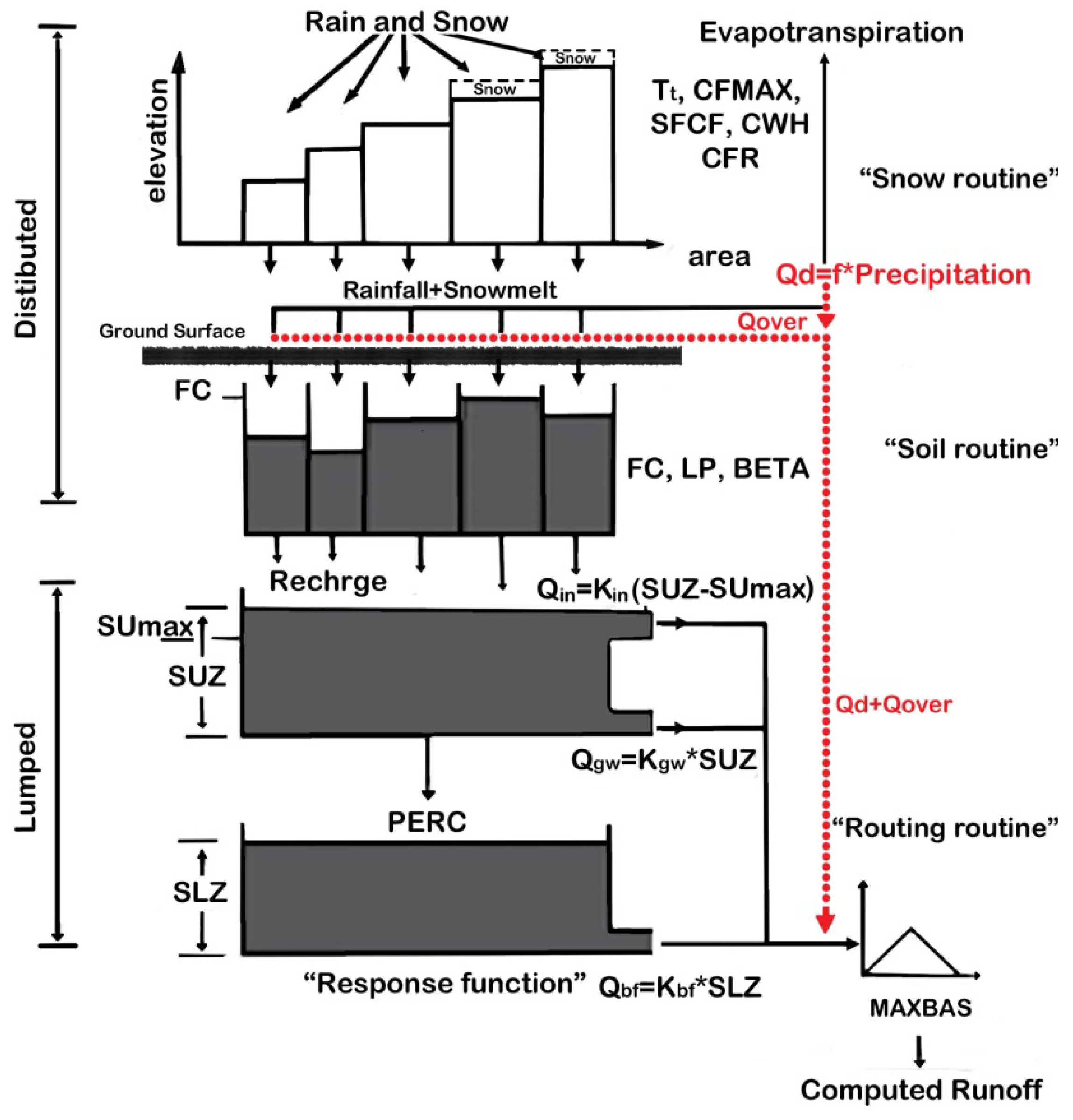
2. Improved HBV Model Description

The HBV conceptual model was initially introduced by Bergstrom in 1976 and has since been used for hydrological simulations, predictions, and water balance studies in more than 30 countries with a wide variety of climates [40]. The HBV model, with a simple and robust structure and a low number of parameters, attempts to cover the most important basin processes that contribute to basin runoff [41]. As shown in Figure 1, in the HBV model, daily discharge is estimated using daily rainfall, air temperature, and the monthly long-term mean potential evaporation [42]. In this model, the simulation of snowmelt flow is carried out using a simple degree-day method while considering snow refreezing and snow hold.
The HBV-Light model version 3.0.0.2, developed by the Geography Department of Zurich University [43,44], carries out the calibration process using Monte-Carlo simulation and Genetic Algorithm. The model is available to the public from University of Zurich (UZH) website [44]. In the present study, researchers have replaced the existing calibration methods with the Shuffle Complex Evolution (SCE) algorithm introduced by Duan et al. [23]. SCE is preferred because it combines the strengths of controlled random search (CRS) algorithms with competitive evolution, and thus proves itself robust, effective, and efficient for a broad class of problems [45]. In the HBV-Light structure that is described in UZH [44], the model does not consider overland flow and estimates snowmelt through a simple degree-day equation. In order to be more compliant with catchment conditions in arid and/or semi-arid regions, some modifications are made on the original HBV-Light structure. In improved HBV (IHBV), overland flow (the dashed line in Figure 1) is calculated by the Green-Ampt infiltration equation (Equation (1)) [46] and snowmelt is estimated using a modified degree-day equation as shown by Equation (2). In this Equation, degree-day factor (Cfmax) is a key parameter that varies by several variables such as air temperature, elevation, snow albedo, solar radiation and so on [47,48]. Thus, the term e g a m a × ( T T t ) is added to simulate the effect of air temperature fluctuations on the degree-day factor.
F = K s × ( 1 + ψ Δ θ S M )
M e l t = C f max × e g a m a × ( T T t ) × ( T T t )
where F is the infiltration rate (mm/day), ψ the wetting front matric potential (mm), Δ θ the change in volumetric moisture content across the wetting front (mm/mm) and SM is soil moisture (mm). In addition, Melt is snowmelt (mm/day) and T is the air temperature.
The range and the description of the remaining parameters in IHBV are shown in Table 1. Because the HBV-Light source code was not available, the authors have developed the IHBV model in FORTRAN. Further information on HBV and its applications can be found in related references [41,49,50,51].

3. Methodology

As noted above, using partitioning scheme in rainfall–runoff models (RR-PS) is a procedure which helps calibrate the model for various streamflow regimes. In the following sections, FCM clustering and SP techniques are explained.

3.1. Clustering Analysis FCM

Cluster analysis using the FCM was initially proposed by Bezdek [35]. This method develops a fuzzy partition providing a degree of membership (μFi) pertinent to each input data point xj to a given cluster Fi. The main advantage of FCM over other clustering methods is that it is less likely to be affected by local minima because it makes soft decisions using membership functions [17]. In FCM method, the membership value of each data point is obtained based on its distance from each cluster centroid. In other words, the membership value of each data point increases the closer it is to the centroid of a cluster [35]. Several indices are proposed to determine the number of optimum clusters [52,53,54]. The most important of these indices are Partition Index (SC) and Separation Index (S) suggested by Bensaid et al. [53]. SC is the ratio of compactness to separation for each cluster c (Equation (3)) and S index shows separation strength among clusters (Equation (4)):
S C ( c ) = i = 1 c k = 1 n μ i k 2 x k v i 2 n i j = 1 C v i v j 2
S ( c ) = i = 1 c k = 1 n μ i k 2 x k v i 2 n min t i ( v i v t 2 )
where μik is the degree of membership of data point xk in cluster c, and v is the cluster centroid. n and ni are the number of data points and the members in each cluster, respectively. A lower value of SC and S indicates a better partition. It is worthy of mention that neither of the two indices are perfect and trustable. Therefore, the number of optimum clusters obtained from these indices have to be checked through the final results of the application where the clustering technique was applied [55] or must be checked against knowledge of the previous records of the dataset. However, there is no general agreement about choosing the number of optimum clusters [17].

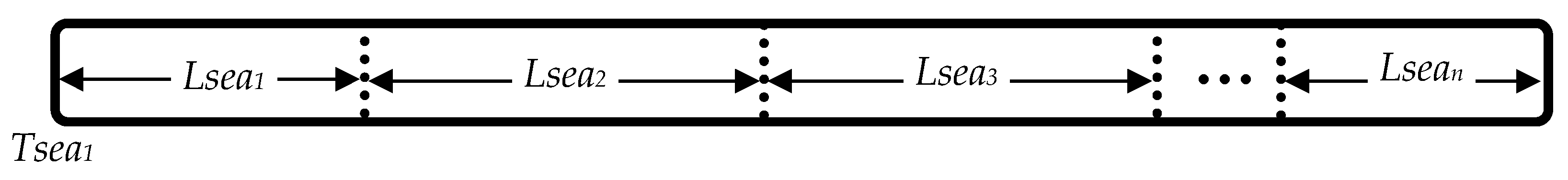
3.2. Seasonal Partitioning (SP) Scheme

The SP is a simple method that can be used for partitioning of input data. In this method, different seasons are defined and the whole modeling period is divided according to these seasons. Then, each input data point is assigned to a season based on its time of occurrence. The starting and ending dates of each season is important for proper parameter calibration. Traditionally, these dates are taken according to the calendar, however, since they vary by geographical and climatological conditions, more precise figures are obtained through calibration.
Thus, in defining seasons, the starting time of the first season and the ending date of the other seasons, except for the last season, must be calibrated similar to other model parameters. Therefore, in SP method with n seasons, one needs to calibrate n additional parameters as compared to the FCM, which could be a drawback of SP, especially in problems with large number of seasons. These parameters include beginning time of the first season (Tsea1) and duration of the first to (n − 1)th season (Lsea1 to Lsean-1) as shown in Figure 2.

3.3. Model Preparation Process
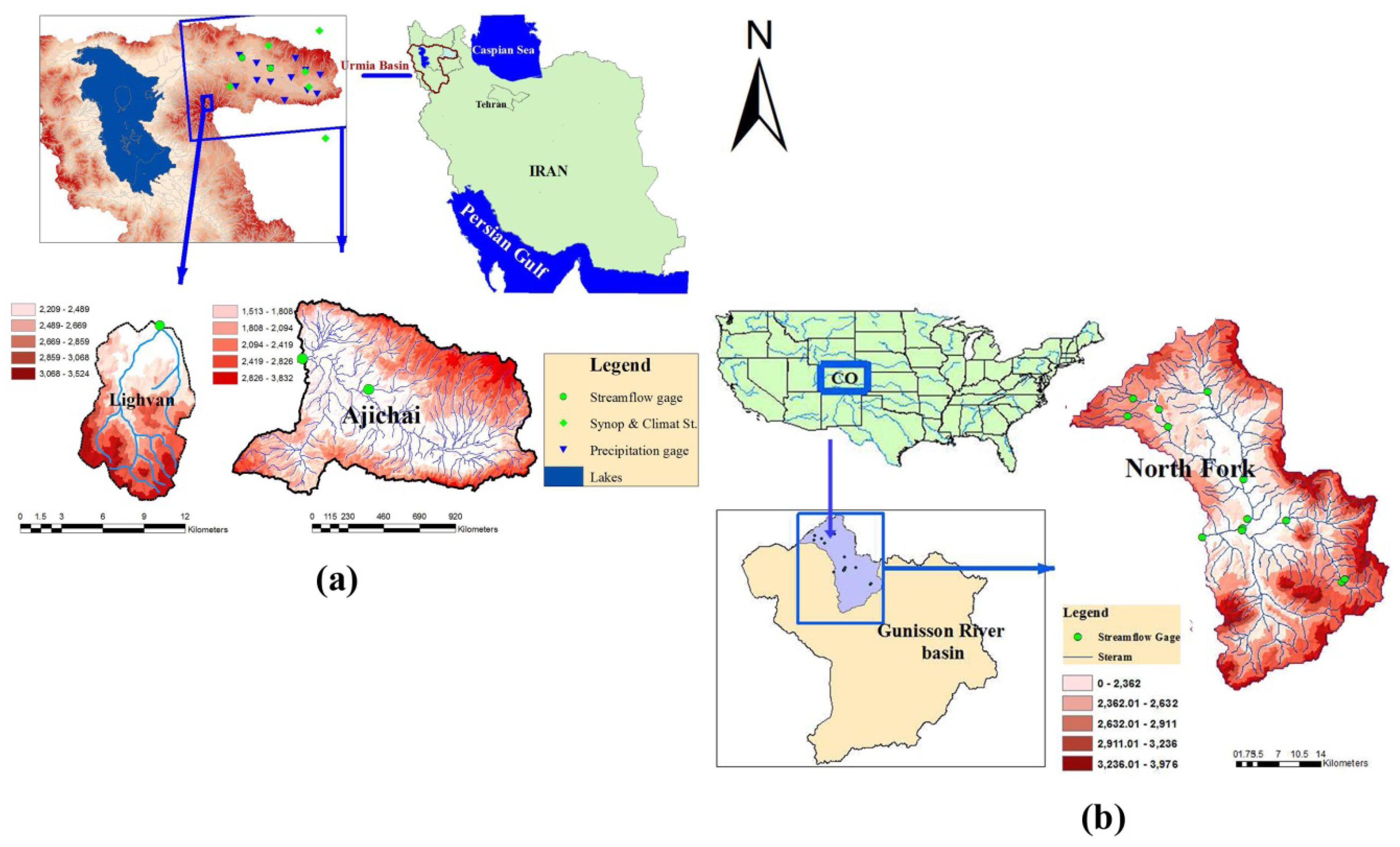
The first step in developing a PS based CRR model is the data separation by either FCM or SP method. In the second step, the model parameters are distinctly defined for each partition. However, as we proceed with partitioning, a problem regarding the growing number of model parameters appears. For example, in a model with n partitions (n clusters or n seasons), the number of parameters becomes n or n+ times the number of parameters in a non-partition model. In order to avoid this problem, we categorized all the model parameters as “sensitive” and “less-sensitive” using a sensitivity analysis.
According to Figure 3, “sensitive” parameters are those that have high impact on the model output and therefore must be calibrated carefully and separately for each season. Similarly, “less-sensitive” parameters have lower impact on the outputs and do not require seasonally separate calibration. Following this procedure, we can reduce the number of model parameters in which otherwise could cause runtime and dimensionality problems.
In this research, an improved HBV model (i.e., IHBV) is used to evaluate the proposed procedures. Then, three data partitioning methods are developed and investigated: (1) the FCM analysis of precipitation and temperature input data (PT); (2) FCM analysis of the selection of extended input data (IS); and (3) Seasonal partitioning (SP). Moreover, the SCE algorithm used in this paper employs two complexes and 35 points in each complex with 3500 iterations and uses the NSE index as the objective function.

4. Study Areas

To calibrate and verify the developed model, three basins in different scales were considered as the study cases. The geophysical and climatological characteristics of these three basins are given in Table 2. Ajichai and Lighvan are the largest and smallest basins of the study, respectively. They are part of larger Urmia Lake basin and are located in Eastern Azerbaijan Province, northwest of Iran (Figure 4a).
Ajichai, which is the main river in Ajichai basin, originates from the southern slopes of Mount Sabalan and, after receiving other branches, drains into Lake Urmia. Lighvan basin originates from the northern slopes of Mount Sahand and its main river is Lighvanchai that joins up with Barichai River at the outlet of the basin (just before Lighvan gage). These basins are located adjacent to each other in a cold and semi-humid climate with dominant snow precipitation during winter months. Therefore, snow melting effectively and significantly contributes to the annual streamflow. The third basin, also with dominant snowfall, is the North Fork Gunnison River near Somerset in Colorado, USA (Figure 4b). It is designated with a hydrologic unit number of 14020004.
Hydroclimatological data includes precipitation, temperature, evaporation and outlet streamflow. Available data for the required duration (see Table 2) for Ajichai and Lighvan basins are taken from Iran Meteorological Organization and Iran Water Resources Management Company. For North Fork, they are obtained from U.S. MOPEX dataset [56].

5. Results and Discussions

In order to evaluate the results, six goodness of fit indices are used as described in Table 3. Nash–Sutcliffe Efficiency (NSE) [57], Root Mean Square Error (RMSE), and Coefficient of Determination (R2) are common indices in evaluating the goodness of fit for rainfall–runoff outputs. However, they lack the ability to correctly evaluate some specific characteristics of the output hydrographs that are of interest for most hydrologists, such as the accuracy of estimates in peak flows.
Although NSE index has been criticized for imposing more weight on higher flows through its quadratic function [58], it cannot evaluate the condition of peak flows independently. Thus, Scharffenberg and Fleming [59] suggested the peak-weighted root mean square error (RMSE-PW) as a single error index for assessing peak flows. However, similar to other error-based indices, RMSE-PW suffers from scale dependency and therefore is not suitable by itself for fitness evaluation. Therefore, we suggest High-Flow and Low-Flow Weighted NSE indices (NSE-HF and NSE-LF) for peak and low flow evaluations. These indices are NSE based with similar range. Linearly distributed weights are used to calculate the RMSE-PW and NSE-HF indices for high flows. Thus, for flows greater than the mean observed streamflow, weights greater than 1.0 are used in calculating these indices. Whereas, for flows equal to or less than the observed mean, linearly distributed weights between 1.0 and 0.5 are applied. Similarly, in calculating NSE-LF indices for low flows, linearly distributed weights more than 1.0 are used for flows that are equal to or less than the mean observed streamflow. Furthermore, linearly distributed weights between 1.0 and 0.5 are applied for flows equal to or more than the mean observed streamflow.

5.1. Sensitivity Analysis Results

Sensitivity analysis describes the impact of variation in the model parameters on the model outputs. To perform this analysis, initially the range of each parameter is determined. Then, the model is executed using an initial set of parameters, which is used as the benchmark for comparison. Next, by keeping other parameters at the initial level, the value of each particular parameter is varied from its lower band (zero percent) to the upper band (100 percent) using increments of five percent. Finally, using the NSE index as the objective function, difference between the current and the initial objective function (ΔOF) is obtained.
As illustrated in Figure 5, the sensitive parameters in each basin are not quite the same. Therefore, sensitive and less-sensitive parameters are separately defined for each basin.
In addition, Figure 5 shows that FC, Kbf and Kperc are common sensitive parameters in all three basins, beta is common in two basins, and each of SFCF, CFmax, TT, and LP are identified as sensitive only in one basin. The sensitivity analysis reveals that sensitive parameters may vary from one basin to another due to hydro-climatic condition of each basin. For example in the North Fork, snowmelt related parameters are more sensitive, while in Lighvan and Ajichai infiltration and temperature parameters are more important.
In order to efficiently run the RR-PS model, the first five sensitive parameters are selected for partitioning (i.e., PS part) while the remaining thirteen less-sensitive parameters are excluded from partitioning and are used in the “regular” part of the model as shown in Figure 3.

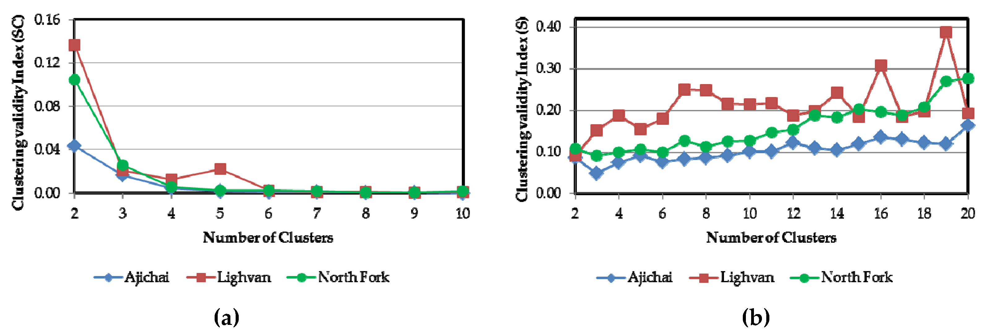
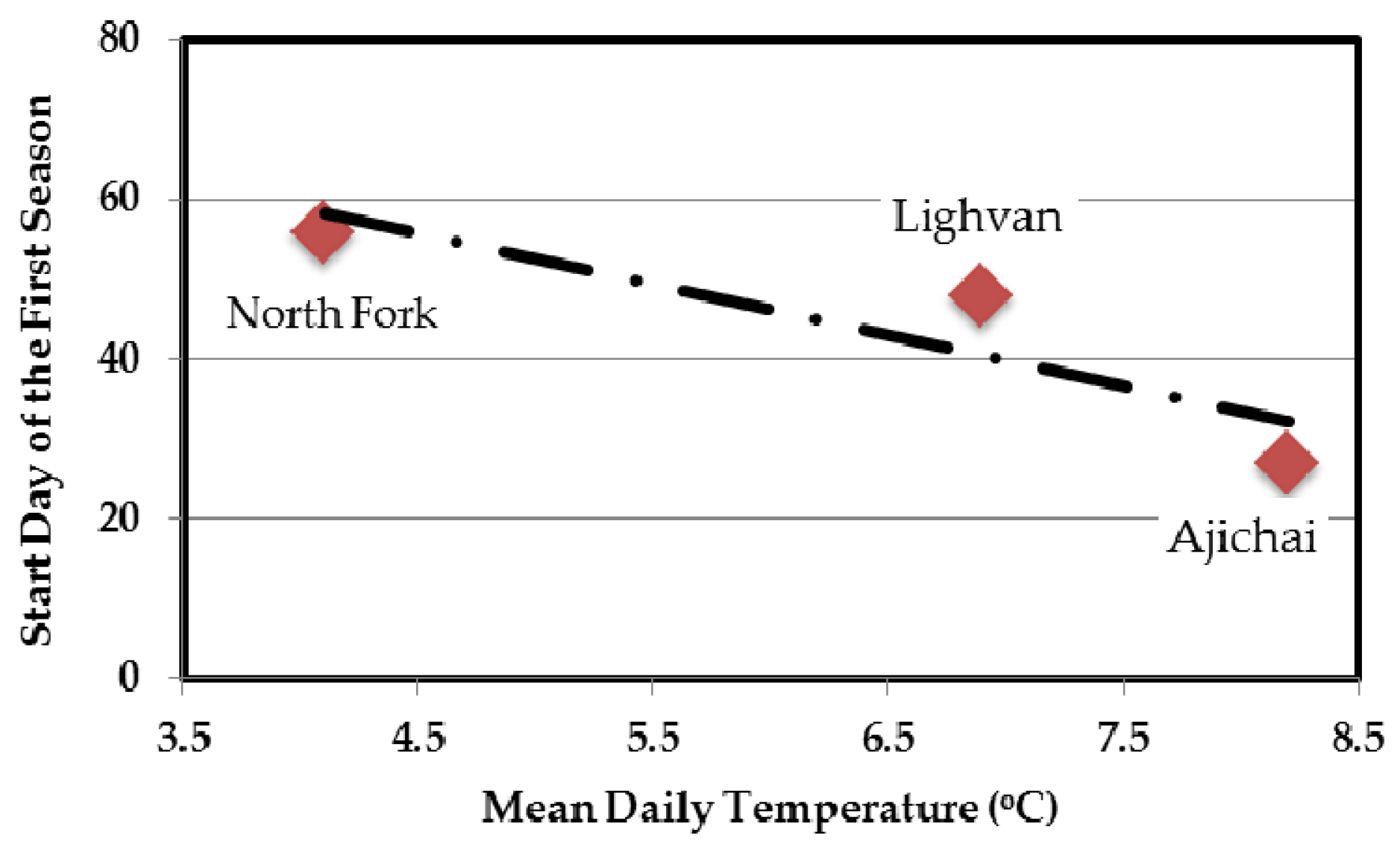
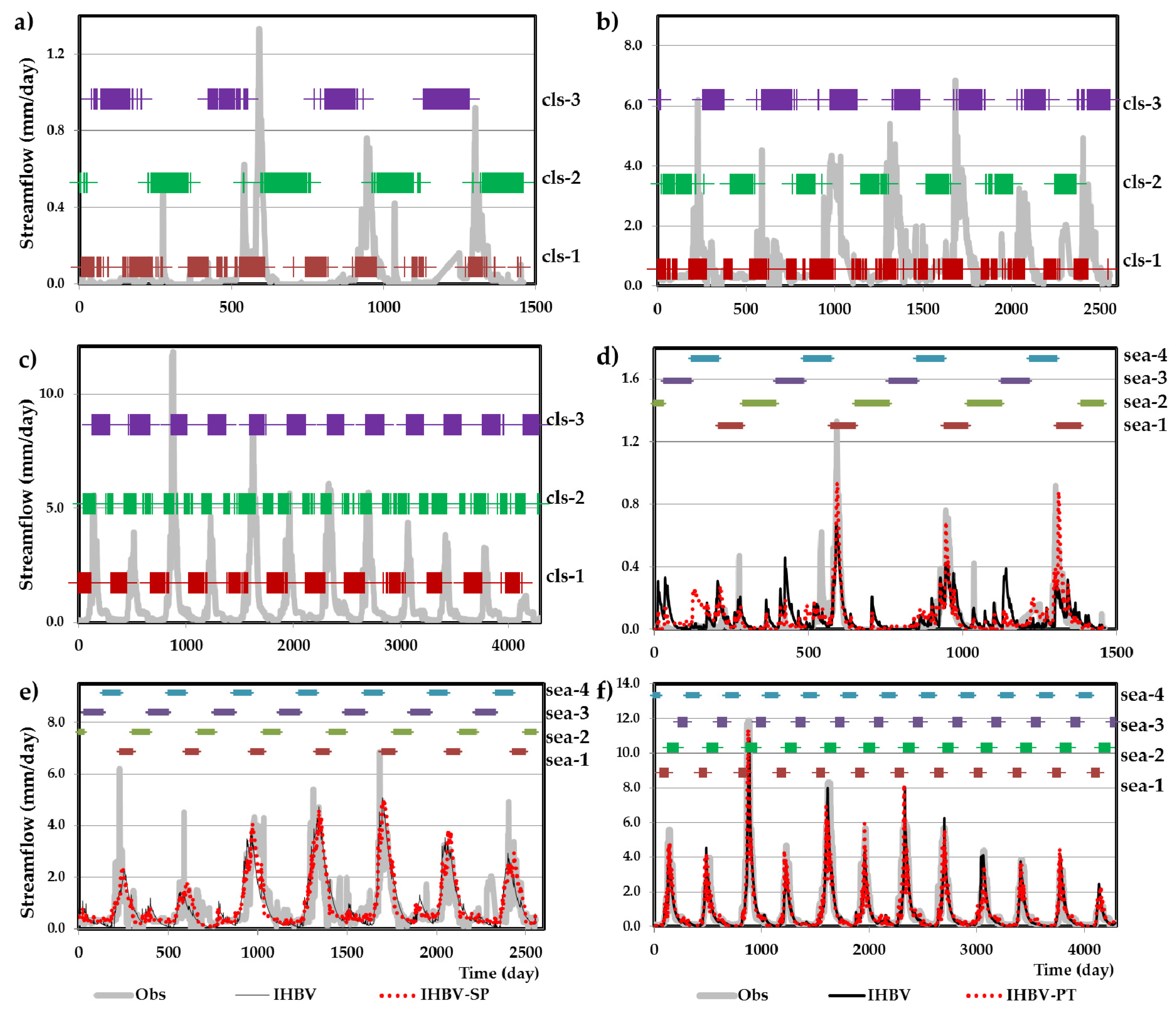
5.2. Data Partitioning Through FCM and SP

As noted earlier, the inputs of FCM are selected in two ways. The first method works based on input data selection (IS). In IS, in addition to the model input data, which are temperature and precipitation, initially accumulatively lagged temperature and precipitation data are also investigate using linear correlation between these parameters and the observed streamflow in each basin.
The optimum lag is then determined for the maximum correlation coefficient for each variable. The results show that the 148-day accumulative temperature data and the 69-day accumulative precipitation data (Tacc148 and Pacc 69) in Ajichai, Pacc 69 in Lighvan and Pacc 219 in North Fork with maximum correlation coefficients are most suitable to be used in the model.
In the second method, FCM analysis is applied using only two inputs, precipitation and temperature data. In the next step, we need to determine the best number of clusters. Figure 6 shows that using S and SC indices, the best number of clusters for all basins is in the range of 2 to 4. To determine the exact number of clusters, the RR-PS model is run with FCM-IS and FCM-PT and for 2, 3, and 4 clusters. The results, as reported in Table 4, reveal that based on both calibration and test NSE indices, in general the most appropriate response is provided by 3 clusters.
Next, the results show that IHBV-SP equipped by user-defined seasons as compared to calendar based season length, has improved NSE index by 35.0%, 9.0%, and 1.2% in calibration period and by 1.5%, 35.0%, and 4.0% in test period for Ajichai, Lighvan and North Fork basins, respectively. It should be noted that the descriptive parameters of user-defined seasons are determined in the calibration process. For example, assuming the calendar year, the calibration results indicate that the first season starts on Day 27, 48, and 56 in Ajichai, Lighvan, and North Fork basins, respectively. Similarly, the length of first season is found to be 78, 71, and 72 days and that of fourth season is found as 88, 95, and 115 days for Ajichai, Lighvan, and North Fork, respectively. As observable, the starting date of the first season as well as the length of each season varies from one basin to another. This could be due to different climatic conditions in each basin. Figure 7 shows that according to our applications there is in fact an inverse correlation between the length of the starting date and the mean daily temperature of basins. As can be seen in Figure 7, basins with the lower mean temperature have later starting dates for the first season. For example, in North Fork basin, with the lowest mean daily temperature (4.1 °C), the starting date of the first season is latest among all (the 56th day of the year); while in Ajichai basin with a mean daily temperature of 8.2 °C, the first season starts on the 27th day of the year. This shows that cold weather is a determining factor in specifying the start of the first season.

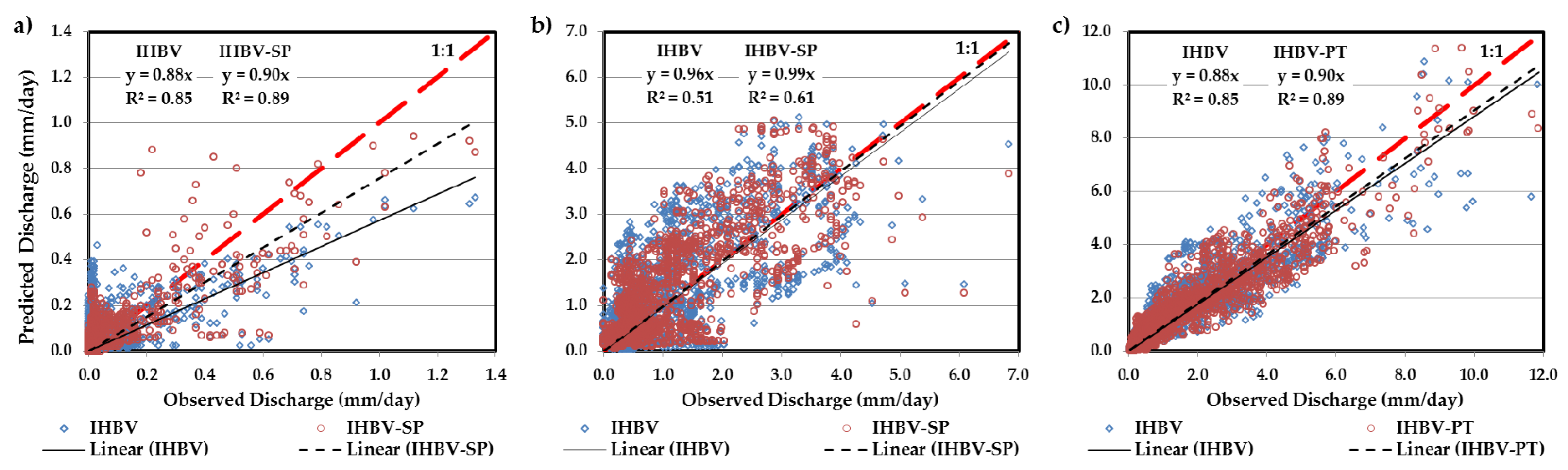
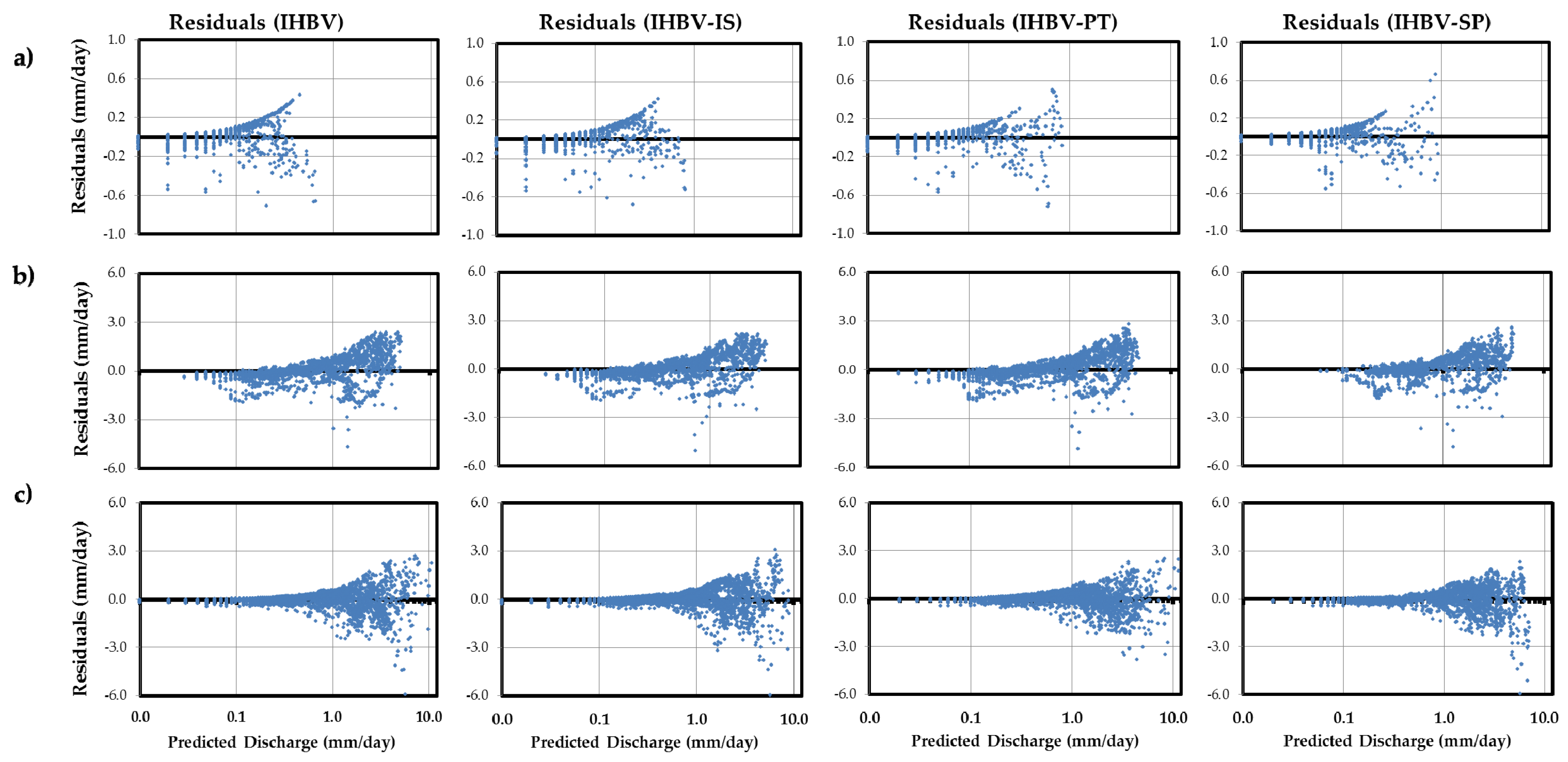
5.3. Comparison of Results

The results in all the three basins are evaluated by the indices stipulated in Table 3. The evaluations show that despite the fact that partitioning scheme (IHBV-SP, IHBV-IS and IHBV-PT) complicates the problem by increasing the number of model parameters, in overall it improves the model results. It is worth mentioning that these findings are in accordance with the literature [60].
As observable from Table 5, except in Ajichai where IHBV has the worst result during the calibration period, HBV-Light is the weakest among all for the other two basins during the same period, and for all the three basins during the test period. In addition, RMSE-PW, NSE-HF, and NSE-LF indices demonstrate that HBV-Light has been the weakest model in both high and low flows. Therefore, the improved version (i.e., IHBV) shows better performance than the original HBV-Light model. Moreover, in all cases, partition-based models perform better than either of the HBV-Light or IHBV models. On the other hand, the results obtained in Ajichai and Lighvan basins show that IHBV-SP has been the most powerful of all the investigated models.
The most improvement by partitioning was obtained in Ajichai basin. In this basin, seasonal partitioning enhanced the amount of NSE, NSE-HF, and NSE-LF indices by 0.23, 0.74, and 0.21 increments, respectively. The performance of IHBV-SP in Lighvan was also better than the other models in both periods. In North Fork, IHBV-PT had the best performance, which could be due to better matching of the defined clusters with the streamflow. However, among the RR-PSs, IHBV-IS shows the weakest performance, which is probably due to utilizing linear correlation as input selection tool. Since the relationship between inputs and the output of a model is not always linear, the linear correlation cannot always make the right choices in the model input selection process (see also [61]).
Figure 8 illustrates a comparison between the results of FCM or SP and the observed streamflow at each basin. As observable from Figure 8c, clusters 1 and 3 (cls-1 and cls-3) match low flows and high flows in North Fork very well, while cls-2 mostly matches middle flows and local peaks. However, as it can be seen from Figure 8a,b the clusters in Ajichai and Lighvan are unable to catch the observed streamflow states as well as they did in North Fork. Therefore, two input based clustering methods, i.e. IHBV-PT and IHBV-IS, show weaker performances in these two basins than the seasonally based IHBV-SP method. Meanwhile, IHBV-SP has been able to provide a good seasonal separation in each of the three basins. Figure 8d–f show that in the test period, middle to high flows mostly occur in seasons 4 and 1, while low to middle flows occur in seasons 2, 3 and 4. This clear separation helps IHBV-SP to have a more precise partitioning and consequently a better model performance.
Figure 9 compares the scatterplots of the results by IHBV and the most suitable model in each basin during the test period. The dashed red line with a slope 1 (i.e., Y = X) shows where the perfect estimation occurs (with zero error). This graph is also used to detect the possible trends in the model outputs. In other words, it can reveal which models underestimate or overestimate the streamflow throughout the observed data range. The other lines are fitted using the outputs of the models as indicated below each figure. According to Figure 9, all the developed models have underestimated the peak flows to some degrees. In Lighvan, the fitted lines of both models (i.e., IHBV and IHBV-SP) are very close to the line with slope 1.
However, the predictions are widely scattered and far from the observed data. In Ajichai (Figure 9a), the model predictions are more tilted downward showing a strong underestimation trend. However, it shows that IHBV-SP has significantly improved the results. Moreover, as can be seen in Figure 9c, in North Fork both IHBV-PT and IHBV models underestimate the peak streamflow with similar performance but less scattered as compared to the other two basins. However, PS models based on FCM analysis (IHBV-PT and IHBV-IS) require partitioning of new input data in each run. While in SP method no addition analysis other than defining the seasons is required. Nevertheless, as mentioned above, the FCM methods are useful when the model input data are suitable for partitioning. On the other hand, for the cases where seasonal variations are important, partitioning based on seasons (i.e., SP) would help to improve the model outputs. In general, partitioning is only useful if there exists a grouping-based behavior within the system.
Another method to evaluate the performance of the CRR models is the assessment of behavior of residuals. Based on maximum likelihood theory, the model residuals must have a mean of zero and constant variance (i.e., homoscedasticity) [62,63]. Figure 10 shows the models’ residuals relative to the predicted discharge during the test period for each basin.
To clarify the behavior of residuals, x-axis is defined logarithmically. By comparing the scattergram of IHBV-IS, IHBV-PT, and IHBV-SP with IHBV, it becomes clear that residuals in all of the models are distributed around zero, although it is not possible to make an explicit judgement about homoscedasticity in the residuals of each RR-PS model. Therefore, it is preferred that homoscedasticity of residuals of each model be tested by the non-parametric Kruskal–Wallis H-test as it follows [64].
H = 12 n ( n + 1 ) i = 1 k R i 2 n i 3 ( n + 1 )
where n is the length of time series, k is the number of classes determined by user, ni is number of residuals located in ith class and Ri is the sum of the ranks occupied by the ni residuals of the ith sample. When ni > 5, the sampling distribution of the H-statistic is fitted approximately by the chi-square distribution with k−1 degrees of freedom. In this test, the acceptance of null hypothesis confirms that k independent random samples come from the same population with similar variance, which is an indication of homoscedasticity.
If H is smaller than the chi-square value with given significance level α and k−1 degrees of freedom, then the null hypothesis is accepted. Table 6 illustrates that with α = 0.05, the null hypothesis for IHBV-SP with k = 5 in Ajichai, and IHBV-SP and IHBV-PT with k = 3 in North Fork basins, would be accepted, proving homoscedasticity in errors. This means that these models, in comparison with IHBV and IHBV-IS, are able to remove the tendency of residuals.
However, homoscedasticity in Lighvan basin for all four models with k = 5 as well as for k = 3, 4, 6, and 7 would be rejected but later cases are not shown here to save space.
Finally, the computational time, using a computer with Intel Core i5-520M processor 2.40 GHZ, in all of the studied models seems reasonably short. For example, the computational time of IHBV-SP for North Fork with the largest number of model parameters (i.e., 38 parameters) and the longest calibration period (15,706 days) is 2280 seconds for 3500 iterations, which is the maximum model execution time among all models and basins. Conversely, the computational time of HBV-Light model with the least number of parameters (15 parameters) for Ajichai basins is 160 seconds, which is the minimum among all. Moreover, the application of IHBV model in Ajichai basin with 19 parameters and with a calibration period of 3287 days, takes only 284 seconds for 3500 iterations. Although the computational time in these models is not too long, it is still possible to reduce it significantly using other state-of-the-art optimization methods such as Surrogate-Enhanced Evolutionary Annealing Simplex Algorithm (SEEAS) or Melody Search (MeS) algorithms [65,66].

6. Conclusions

This paper demonstrated the application of an improved conceptual model (i.e., IHBV) along with partitioning scheme to minimize the streamflow prediction errors. To avoid excessive increase of the model parameters, sensitivity analysis was used to identify sensitive and less-sensitive parameters. Then, only sensitive parameters were used in the partitioning module and less-sensitive parameters were calibrated using the regular method with the whole data. Furthermore, the application of three partitioning methods including a seasonal partitioning (IHBV-SP) and two input data partitioning by Fuzzy C-Means (i.e., IHBV-IS and IHBV-PT) along with the simple IHBV model were investigated and compared. The results show that among developed models, IHBV-SP had the best performance in Ajichai and Lighvan while IHBV-PT performed better in North Fork. IHBV-IS had the weakest performance among all the partitioning methods, which could partly be due to shortcomings of the linear correlation based input data selection method.
Moreover, complementary analysis on model residuals showed that they have a mean near zero. In addition, the application of Kruskal–Wallis H-test proved the homoscedasticity for IHBV-SP with k = 5 in Ajichai, and IHBV-SP and IHBV-PT with k = 3 in North Fork basins. However, the homoscedasticity condition in Lighvan basin was not evidenced.

Acknowledgment

We would like to appreciate the Water Research Institute (WRI) of Iran for providing part of the publication cost of this paper as open access.

Author Contributions

This research article is part of the Ph.D. thesis of the co-author, Mohamad M. Javadianzadeh under the supervision of the first author, Alireza B. Dariane.

Conflicts of Interest

The authors declare no conflict of interest.

References

  1. Wheater, H.; Sorooshian, S.; Sharma, K.D. Hydrological Modelling in Arid and Semi-Arid Areas; Cambridge University Press: Cambridge, UK, 2007. [Google Scholar]
  2. Manley, R. Simulation of flows in ungauged basins/simulation d'écoulement sur les bassins versants non jaugés. Hydrol. Sci. J. 1978, 23, 85–101. [Google Scholar] [CrossRef]
  3. Wagener, T.; Wheater, H.S.; Gupta, H.V. Rainfall-Runoff Modelling in Gauged and Ungauged Catchments; Imperial College Press: Londen, UK, 2004. [Google Scholar]
  4. Loucks, D.P.; Van Beek, E.; Stedinger, J.R.; Dijkman, J.P.; Villars, M.T. Water Resources Systems Planning and Management: An Introduction to Methods, Models and Applications; United Nations Educational, Scientific and Cultural Organization (UNESCO): Paris, France, 2005. [Google Scholar]
  5. Moore, R. Real-Time Flood Forecasting Systems: Perspectives and Prospects; Springer: New York, NY, USA, 1999. [Google Scholar]
  6. Parkin, G.; O'donnell, G.; Ewen, J.; Bathurst, J.; O'Connell, P.; Lavabre, J. Validation of catchment models for predicting land-use and climate change impacts. 2. Case study for a mediterranean catchment. J. Hydrol. 1996, 175, 595–613. [Google Scholar] [CrossRef]
  7. Yu, P.-S.; Yang, T.-C.; Wu, C.-K. Impact of climate change on water resources in southern Taiwan. J. Hydrol. 2002, 260, 161–175. [Google Scholar] [CrossRef]
  8. Shrestha, D.L. Uncertainty Analysis in Rainfall-Runoff Modelling: Application of Machine Learning Techniques. Ph.D. Thesis, Delft University of Technology, Delft, The Netherlands, 2009. [Google Scholar]
  9. Lee, H.; McIntyre, N.; Wheater, H.; Young, A. Selection of conceptual models for regionalisation of the rainfall-runoff relationship. J. Hydrol. 2005, 312, 125–147. [Google Scholar] [CrossRef]
  10. Gourley, J.J.; Vieux, B.E. A method for identifying sources of model uncertainty in rainfall-runoff simulations. J. Hydrol. 2006, 327, 68–80. [Google Scholar] [CrossRef]
  11. Straten, G.; Keesman, K.J. Uncertainty propagation and speculation in projective forecasts of environmental change: A lake-eutrophication example. J. For. 1991, 10, 163–190. [Google Scholar] [CrossRef]
  12. Efstratiadis, A.; Koutsoyiannis, D. One decade of multi-objective calibration approaches in hydrological modelling: A review. Hydrol. Sci. J. 2010, 55, 58–78. [Google Scholar] [CrossRef]
  13. Kim, Y.; Chung, E.-S.; Won, K.; Gil, K. Robust parameter estimation framework of a rainfall-runoff model using Pareto optimum and minimax regret approach. Water 2015, 7, 1246. [Google Scholar] [CrossRef]
  14. Gupta, H.V.; Sorooshian, S.; Yapo, P.O. Toward improved calibration of hydrologic models: Multiple and noncommensurable measures of information. Water Resour. Res. 1998, 34, 751–763. [Google Scholar] [CrossRef]
  15. Yang, J.; Reichert, P.; Abbaspour, K.C.; Xia, J.; Yang, H. Comparing uncertainty analysis techniques for a SWAT application to the Chaohe basin in China. J. Hydrol. 2008, 358, 1–23. [Google Scholar] [CrossRef]
  16. Abbaspour, K.C.; Yang, J.; Maximov, I.; Siber, R.; Bogner, K.; Mieleitner, J.; Zobrist, J.; Srinivasan, R. Modelling hydrology and water quality in the pre-alpine/alpine Thur watershed using SWAT. J. Hydrol. 2007, 333, 413–430. [Google Scholar] [CrossRef]
  17. Choi, H.T.; Beven, K. Multi-period and multi-criteria model conditioning to reduce prediction uncertainty in an application of topmodel within the GLUE framework. J. Hydrol. 2007, 332, 316–336. [Google Scholar] [CrossRef]
  18. Beven, K.; Binely, A. The future of distributed model: Calibration and uncertainty prediction. Hydrol. Process. 1992, 6, 279–298. [Google Scholar] [CrossRef]
  19. Jung, Y.; Merwade, V.; Kim, S.; Kang, N.; Kim, Y.; Lee, K.; Kim, G.; Kim, H.S. Sensitivity of subjective decisions in the GLUE methodology for quantifying the uncertainty in the flood inundation map for Seymour reach in Indiana, USA. Water 2014, 6, 2104–2126. [Google Scholar] [CrossRef]
  20. Xiong, L.; Shamseldin, A.Y.; O'Connor, K.M. A non-linear combination of the forecastes of rainfall-runoff models by the first-order Takagi-Sugeno fuzzy system. J. Hydrol. 2001, 245, 196–217. [Google Scholar] [CrossRef]
  21. Ajami, N.K.; Duan, Q.; Sorooshian, S. An integrated hydrologic bayesian multimodel combination framework: Confronting input, parameter, and model structural uncertainty in hydrologic prediction. Water Resour. Res. 2007, 43. [Google Scholar] [CrossRef]
  22. Duan, Q.; Ajami, N.K.; Gao, X.; Sorooshian, S. Multi-model ensemble hydrologic prediction using bayesian model averaging. Adv. Water Resour. 2007, 30, 1371–1386. [Google Scholar] [CrossRef]
  23. Duan, Q.; Gupta, V.K.; Sorooshian, S. Shuffled complex evolution approach for effective and efficient global minimization. J. Optimization Theory Appl. 1993, 76, 501–521. [Google Scholar] [CrossRef]
  24. Liu, Y. Automatic calibration of a rainfall–runoff model using a fast and elitist multi-objective particle swarm algorithm. Expert Syst. Appl. 2009, 36, 9533–9538. [Google Scholar] [CrossRef]
  25. Seong, C.; Her, Y.; Benham, B.L. Automatic calibration tool for hydrologic simulation program-fortran using a shuffled complex evolution algorithm. Water 2015, 7, 503–527. [Google Scholar] [CrossRef]
  26. Gan, T.Y.; Biftu, G.F. Automatic calibration of conceptual rainfall-runoff models: Optimization algorithms, catchment conditions, and model structure. Water Resour. Res. 1996, 32, 3513–3524. [Google Scholar] [CrossRef]
  27. Abbaspour, K.; Johnson, C.; Van Genuchten, M.T. Estimating uncertain flow and transport parameters using a sequential uncertainty fitting procedure. Vadose Zone J. 2004, 3, 1340–1352. [Google Scholar] [CrossRef]
  28. Berhanu, B.; Seleshi, Y.; Demisse, S.S.; Melesse, A.M. Flow regime classification and hydrological characterization: A case study of ethiopian rivers. Water 2015, 7, 3149–3165. [Google Scholar] [CrossRef]
  29. Ferket, B.V.A.; Samain, B.; Pauwels, V.R.N. Internal validation of conceptual rainfall–runoff models using baseflow separation. J. Hydrol. 2010, 381, 158–173. [Google Scholar] [CrossRef]
  30. Wagener, T.; McIntyre, N.; Lees, M.; Wheater, H.; Gupta, H. Towards reduced uncertainty in conceptual rainfall-runoff modelling: Dynamic identifiability analysis. Hydrol. Process. 2003, 17, 455–476. [Google Scholar] [CrossRef]
  31. Boyle, D.P.; Gupta, H.V.; Sorooshian, S. Toward improved calibration of hydrologic models: Combining the strengths of manual and automatic methods. Water Resour. Res. 2000, 36, 3663–3674. [Google Scholar] [CrossRef]
  32. Bradley, P.S.; Fayyad, U.M. Refining Initial Points for K-Means Clustering. In Proceedings of the International Conference on Machine Learning (ICML 98), Madison, WI, USA, 1998; pp. 91–99.
  33. Vos, N.J.D.; Rientjes, T.H.M.; Gupta, H.V. Diagnostic evaluation of conceptual rainfall–runoff models using temporal clustering. Hydrol. Process. 2010, 24, 2840–2850. [Google Scholar] [CrossRef]
  34. Wu, C.L.; Chau, K.W. Prediction of rainfall time series using modular soft computing methods. Eng. Appl. Artif. Intell. 2012, 26, 997–1007. [Google Scholar] [CrossRef]
  35. Bezdek, J.C. Cluster validity with fuzzy sets. J. Cybern. 1973, 3, 58–73. [Google Scholar] [CrossRef]
  36. Fleming, M.; Neary, V. Continuous hydrologic modeling study with the hydrologic modeling system. J. Hydrol. Eng. 2004, 9, 175–183. [Google Scholar] [CrossRef]
  37. Nilsson, P.; Uvo, C.B.; Berndtsson, R. Monthly runoff simulation: Comparing and combining conceptual and neural network models. J. Hydrol. 2006, 321, 344–363. [Google Scholar] [CrossRef]
  38. Garbrecht, J.D. Comparison of three alternative ann designs for monthly rainfall-runoff simulation. J. Hydrol. Eng. 2006, 11, 502–505. [Google Scholar] [CrossRef]
  39. Seasholtz, M.B.; Kowalski, B. The parsimony principle applied to multivariate calibration. Anal. Chim. Acta 1993, 277, 165–177. [Google Scholar] [CrossRef]
  40. Lindström, G.; Johansson, B.; Persson, M.; Gardelin, M.; Bergström, S. Development and test of the distributed HBV-96 hydrological model. J. Hydrol. 1997, 201, 272–288. [Google Scholar] [CrossRef]
  41. Abebe, N.A.; Ogden, F.L.; Pradhan, N.R. Sensitivity and uncertainty analysis of the conceptual HBV rainfall–runoff model: Implications for parameter estimation. J. Hydrol. 2010, 389, 301–310. [Google Scholar] [CrossRef]
  42. Seibert, J. Regionalisation of parameters for a conceptual rainfall-runoff model. Agric. For. Meteorol. 1999, 98, 279–293. [Google Scholar] [CrossRef]
  43. Seibert, J. HBV Light, Version 2, User’s Manual; Department of Physical Geography and Quaternary Geology, Stockholm University: Stockholm, Sweden, 2005. [Google Scholar]
  44. HBV Light Model; software for catchment runoff simulation; University of Zurich (UZH): Zurich, Switherland. Available online: http://www.geo.uzh.ch/en/units/h2k/services/hbv-model (accessed on 5 July 2014).
  45. Jeon, J.-H.; Park, C.-G.; Engel, B.A. Comparison of performance between genetic algorithm and SCE-UA for calibration of SCS-CN surface runoff simulation. Water 2014, 6, 3433–3456. [Google Scholar] [CrossRef]
  46. Rawls, W.J.; Brakensiek, D.L.; Miller, N. Green-Ampt infiltration parameters from soils data. J. Hydraulic Eng. 1983, 109, 62–70. [Google Scholar] [CrossRef]
  47. Hock, R. Temperature index melt modelling in mountain areas. J. Hydrol. 2003, 282, 104–115. [Google Scholar] [CrossRef]
  48. Li, X.; William, M.W. Snowmelt runoff modelling in an arid mountain watershed, Tarim Basin, China. Hydrol. Process. 2008, 22, 3931–3940. [Google Scholar] [CrossRef]
  49. Braun, L.N.; Renner, C.B. Application of a conceptual runoff model indifferent physiographic regions of Switzerland. Hydrol. Sci. J. 1992, 37, 217–231. [Google Scholar] [CrossRef]
  50. Seibert, J. Conceptual Runoff Models—Fiction or Representation of Reality? Ph.D. Thesis, Uppsala University, Uppsala, Sweden, 1999. [Google Scholar]
  51. Vis, M.; Knight, R.; Pool, S.; Wolfe, W.; Seibert, J. Model calibration criteria for estimating ecological flow characteristics. Water 2015, 7, 2358–2381. [Google Scholar] [CrossRef]
  52. Bezdek, J.C.; Ehrlich, R.; Full, W. FCM: The fuzzy c-means clustering algorithm. Comput. Geosci. 1984, 10, 191–203. [Google Scholar] [CrossRef]
  53. Bensaid, A.M.; Hall, L.O.; Bezdek, J.C.; Clarke, L.P.; Silbiger, M.L.; Arrington, J.A.; Murtagh, R.F. Validity-guided (re) clustering with applications to image segmentation. IEEE Trans.Fuzzy Syst. 1996, 4, 112–123. [Google Scholar] [CrossRef]
  54. Xie, X.L.; Beni, G. A validity measure for fuzzy clustering. IEEE Trans. Pattern Anal. Mach. Intell. 1991, 13, 841–847. [Google Scholar] [CrossRef]
  55. Shrestha, D.L.; Solomatine, D.P. Data-driven approaches for estimating uncertainty in rainfall-runoff modelling. Intl. J. River Basin Manag. 2008, 6, 109–122. [Google Scholar] [CrossRef]
  56. Schaake, J.; Cong, S.; Duan, Q. The USA MOPEX data set. IAHS Publ. 2006, 307, 9. [Google Scholar]
  57. Nash, J.E.; Sutcliffe, J.V. River flow forecasting throligh conceptual models part I—A disclission of principles. J. Hydrol. 1970, 10, 282–290. [Google Scholar] [CrossRef]
  58. Legates, D.R.; McCabe, G.J., Jr. Evaluating the use of "goodness-of-fit" measures in hydrologic and hydroclimatic model validation. Water Resour. Res. 1999, 35, 233–241. [Google Scholar] [CrossRef]
  59. Scharffenberg, W.; Ely, P.; Daly, S.; Fleming, M.; Pak, J. Hydrologic modeling system (HEC-HMS): Physically-based simulation components. In Proceedings of the 2nd Joint Federal Interagency Conference, Las Vegas, NV, USA, 27 June–1 July 2010; p. 8.
  60. Her, Y.; Chaubey, I. Impact of the numbers of observations and calibration parameters on equifinality, model performance, and output and parameter uncertainty. Hydrol. Process. 2015, 29, 4220–4237. [Google Scholar] [CrossRef]
  61. Maier, H.R.; Jain, A.; Dandy, G.C.; Sudheer, K.P. Methods used for the development of neural networks for the prediction of water resource variables in river systems: Current status and future directions. Environ. Model. Softw. 2010, 25, 891–909. [Google Scholar] [CrossRef]
  62. Sorooshian, S.; Dracup, J.A. Stochastic parameter estimation procedures for hydrologie rainfall-runoff models: Correlated and heteroscedastic error cases. Water Resour. Res. 1980, 16, 430–442. [Google Scholar] [CrossRef]
  63. Xu, C. Statistical analysis of parameters and residuals of a conceptual water balance model—Methodology and case study. Water Resour. Manag. 2001, 15, 75–92. [Google Scholar] [CrossRef]
  64. Kruskal, W.H.; Wallis, W.A. Use of ranks in one-criterion variance analysis. J. Am. Stat. Assoc. 1952, 47, 583–621. [Google Scholar] [CrossRef]
  65. Ashrafi, S.; Dariane, A. Performance evaluation of an improved harmony search algorithm for numerical optimization: Melody Search (MS). Eng. Appl. Artif. Intell. 2013, 26, 1301–1321. [Google Scholar] [CrossRef]
  66. Tsoukalas, I.; Kossieris, P.; Efstratiadis, A.; Makropoulos, C. Surrogate-enhanced evolutionary annealing simplex algorithm for effective and efficient optimization of water resources problems on a budget. Environ. Model. Softw. 2016, 77, 122–142. [Google Scholar] [CrossRef]
Figure 1. Improved HBV (IHBV) diagram.
Water 08 00063 g001
Figure 2. Season definition.
Water 08 00063 g002
Figure 3. Diagram of Rainfall Runoff-Partitioning Scheme (RR-PS) model.
Water 08 00063 g003
Figure 4. Map of study area: (a) Ajichai and Lighvan basins located in East Azerbaijan province, Iran; and (b) North Fork Gunnison River, in Colorado, USA.
Water 08 00063 g004
Figure 5. Sensitivity analysis in different basins: (a) Ajichai; (b) Lighvan; and (c) North Fork.
Water 08 00063 g005
Figure 6. Comparison of clustering validity index by (a) Partition Index (SC) and (b) Separation Index (S).
Water 08 00063 g006
Figure 7. Relation between starting date and the mean daily temperature.
Water 08 00063 g007
Figure 8. Comparison of different clustering levels in (a) Ajichai; (b) Lighvan; and (c) North Fork; and comparison of IHBV-SP results with the observed flow in (d) Ajichai; (e) Lighvan; and (f) North Fork in test period.
Water 08 00063 g008
Figure 9. The scatterplots of the results by IHBV and the most suitable model during the test period and in: (a) Ajichai; (b) Lighvan; and (c) North Fork.
Water 08 00063 g009
Figure 10. Scattergrams of residuals during test period: (a) Ajichai; (b) Lighvan; and (c) North Fork.
Water 08 00063 g010
Table 1. The parameters of IHBV model.
ParameterDescriptionUnitRange
Snow Routine:
TtThreshold Temperature[°C]−2.0–3.0
CfmaxDegree-Day factor[mm/(°C day)]0.0–10.0
SFCFSnowfall correction factor[-]0.5–1.5
CFRRefreezing coefficient[-]0.0–1.0
CWHWater holding capacity[-]0.0–6.0
gamaCorrection factor[-]0.0–0.5
Soil Routine:
KsConductivity coefficient[mm/day]0.0–200
ns= ψ Δ θ [mm]0.1–0.6
FCMaximum of soil moisture (SM)[mm]0.1–900.0
cepEvaporation correction factor[-]0.0–1.0
betaShape coefficient[-]0.0–7.5
LPThreshold for reduction of evaporation (SM/FC)[-]0.0–1.0
Response Routine:
SUmaxThreshold for Kin-outflow[mm]5.0–1000.0
PercMaximal flow from upper to lower box[mm/day]0.0–15.0
KinRecession coefficient (Upper storage)[1/day]0.0–10.0
KgwRecession coefficient 1 (Lower storage)[1/day]0.0–0.2
KbfRecession coefficient 2 (Lower storage)[1/day]0.0–0.2
MaxBasRouting, length of weighting function[day]1.0–10.0
Table 2. Geophysical and climatological characteristics of the basins.
DescriptionBasin Name
AjichaiLighvanNorth Fork
LocationsUrmia Basin, East Azerbaijan, IranUrmia Basin, East Azerbaijan, IranNorth Fork Gunnison River, CO, USA
Latitude37°45’–38°19’ N37°45’–37°50’ N38°42’–39°15’ N
Longitude46°48’–47°52’ E46°25’–46°26’ E107°05’–107°41’ W
Minimum Altitude151321401914
Maximum Altitude383236203976
Area, km25660.076.51362.3
Annual Precipitation, mm410.8396.1674.6
Annual Runoff, mm25.5329.4278.3
Annual Pot. Evaporation, mm988.91201.81015.7
Mean Annual Temperature, °C 8.26.94.1
Data Period1 Oct 1999–30 Sep 20121 Oct 1979–30 Sep 20061 Oct 1948–30 Sep 2002
Calibration Period1 Oct 1999–30 Sep 20081 Oct 1979–30 Sep 19981 Oct 1948–31 Dec 1990
Validation Period1 Oct 2008–30 Sep 20121 Oct 1999–30 Sep 20061 Jan 1991–30 Sep 2002
Table 3. Goodness of fit indices to compare the results.
NameEquationRange
1Nash-Sutcliffe Efficiency N S E = 1 - i = 1 N ( Q o b s i - Q s i m i ) 2 / i = 1 N ( Q o b s i - Q ¯ o b s ) 2 -∞ To 1
2Root Mean Square Error R M S E = 1 N i = 1 N ( Q o b s i - Q s i m i ) 2 0 To +∞
3Peak-Weighted
Root Mean Square Error
R M S E - P W = 1 N i = 1 N ( Q o b s i + Q ¯ o b s ) ( 2 Q ¯ o b s ) ( Q o b s i - Q s i m i ) 2 0 To +∞
4High Flow Weighted NSE N S E - H F = 1 - i = 1 N [ W H F i × ( Q o b s i - Q s i m i ) 2 ] i = 1 N ( Q o b s i - Q ¯ o b s ) 2 W H F i = Q o b s i + Q ¯ o b s 2 Q ¯ o b s -∞ To 1
5Low Flow Weighted NSE N S E - L F = 1 - i = 1 N [ W L F i × ( Q o b s i - Q s i m i ) 2 ] i = 1 N ( Q o b s i - Q ¯ o b s ) 2 W L F i = ( Q o b s min - Q ¯ o b s ) ( Q o b s i - Q ¯ o b s ) 2 Q ¯ o b s ( Q o b s max - Q ¯ o b s ) + 1 -∞ To 1
6Determination Coefficient R 2 = [ i = 1 N ( Q o b s i - Q ¯ o b s ) × ( Q s i m i - Q ¯ s i m ) i = 1 T ( Q o b s i - Q ¯ o b s ) 2 × t = 1 T ( Q s i m i - Q ¯ s i m ) 2 ] 2 0 To 1
Note: Q o b s i , Q s i m i , Q o b s , Q s i m , Q o b s M i n and Q o b s M a x are the observed flow, simulated flow, average flow, average simulated flow and the smallest and the largest observed flow in the period, respectively.
Table 4. Comparison of Nash-Sutcliffe Efficiency (NSE) indices of HBV model.
ClustersFCMMethodCalibration NSETest NSE
AjichaiLighvanNorth ForkAjichaiLighvanNorth Fork
2IS0.420.670.810.580.130.87
2PT0.510.680.830.490.390.87
3IS0.520.680.820.580.440.85
3PT0.580.640.850.530.410.89
4IS0.570.680.800.310.410.85
4PT0.540.670.870.570.340.87
Table 5. Comparison of results for all the basins.
Evaluation IndexAjichaiLighvanNorth Fork
HBV-LightIHBVIHBV-ISIHBV-PTIHBV-SPHBV-LightIHBVIHBV-ISIHBV-PTIHBV-SPHBV-LightIHBVIHBV-ISIHBV-PTIHBV-SP
I. Calibration Period
NSE0.560.420.520.600.730.570.660.680.640.720.760.790.820.850.83
RMSE0.120.130.120.110.090.670.590.580.610.540.660.620.570.530.56
RMSE-PW0.300.350.340.270.220.900.810.810.870.761.161.050.980.881.00
NSE-HFW−1.88-3.02-2.65-1.38−0.500.220.370.370.280.440.270.400.470.570.45
NSE-LFW0.630.510.600.650.770.630.710.730.700.760.800.820.850.860.85
R20.570.420.520.600.730.630.670.700.660.730.760.790.820.850.83
II. Test Period
NSE0.330.420.560.580.650.280.360.440.410.500.830.850.850.890.87
RMSE0.120.110.090.090.080.760.710.670.680.630.560.510.510.450.48
RMSE-PW0.230.190.160.180.150.890.880.850.840.801.010.880.870.740.86
NSE-HFW1.57-0.91−0.31−0.71−0.170.000.020.100.100.200.440.570.580.690.59
NSE-LFW0.420.480.610.650.690.320.410.490.460.540.860.870.870.900.89
R20.350.430.570.600.660.600.530.600.570.620.830.850.850.890.87
The bold and underlined values indicate the best and the worst values, respectively.
Table 6. The value of H-test for residuals of the models.
BasinK χ 1 α , k 1 2 H-test
IHBVIHBV-ISIHBV-PTIHBV-SP
Ajichai59.49134.0138.456.48.0
Lighvan59.49546.4547.1484.8662.8
North Fork35.9920.333.51.41.0
The bold values indicate where the null hypothesis is accepted.

