Case Study: Effect of Climatic Characterization on River Discharge in an Alpine-Prealpine Catchment of the Spanish Pyrenees Using the SWAT Model

Abstract

The new challenges in assessment of water resources demand new approaches and tools, such as the use of hydrologic models, which could serve to assist managers in the prediction, planning and management of catchment water supplies in view of increased demand of water for irrigation and climatic change. Good characterization of the spatial patterns of climate variables is of paramount importance in hydrological modelling. This is especially so when modelling mountain environments which are characterized by strong altitudinal climate gradients. However, very often there is a poor distribution of climatic stations in these areas, which in many cases, results in under representation of high altitude areas with respect to climatic data. This results in the poor performance of the models. In the present study, the Soil and Water Assessment Tool (SWAT) model was applied to the Barasona reservoir catchment in the Central Spanish Pyrenees in order to assess the influence of different climatic characterizations in the monthly river discharges. Four simulations with different input data were assessed, using only the available climate data (A1); the former plus one synthetic dataset at a higher altitude (B1); and both plus the altitudinal climate gradient (A2 and B2). The model’s performance was evaluated against the river discharges for the representative periods of 2003–2005 and 1994–1996 by means of commonly used statistical measures. The best results were obtained using the altitudinal climate gradient alone (scenario A2). This study provided insight into the importance of taking into account the sources and the spatial distribution of weather data in modelling water resources in mountainous catchments.

1. Introduction

Future scenarios for water resources in the Mediterranean region foresee changes in reservoir inputs, including lower available discharges from dams to meet the water demand from irrigated and urban areas [1]. Water ecosystems are vulnerable to various forms of pressure caused by human activities and they are particularly vulnerable to climate change, all of which may affect water resources and demand. Therefore, hydrological studies are necessary to implement basin management plans to protect water resources. Contemporary catchment models have become very useful tools and the Soil and Water Assessment Tool (SWAT) model is one of the most widely used of the many catchment models available (e.g., [2]). Since it has been continuously improved over the last 30 years, it has gained international acceptance as an interdisciplinary tool suitable for application at different scales of catchments with varying degrees of biophysical and climatic settings (e.g., [3]). However, despite the increasing use of the model, to date the majority of SWAT applications have been carried out in the U.S. and other European regions, which are generally considered to be data-rich compared to other countries (e.g., snow, soil or/and crop data are not available in many countries).

Since spatial and temporal climate variability are key characteristics in hydrologic modelling [4], distributed hydrological models like SWAT require a minimum of daily distributed meteorological data to adequately simulate the hydrological cycle. The drawback is that long-term continuous data are not available in many parts of the world. Given the fact that climate data is a major driver of hydrological and other processes simulated by the model, studies evaluating the impact of climatic input data on SWAT simulations are gaining increased attention. Gassman et al. [3] indicate that poor results can be attributed to inadequate representation of rainfall inputs, either due to a lack of adequate rain gauges in the simulated catchment or to subcatchment configurations that are too coarse to capture the spatial detail of rainfall inputs [5]. The impact of rain gauge density, the distribution of stations in the catchment, and the data sources for generating climate inputs have also been studied [6,7].

Modelling hydrology is a difficult task to perform accurately in terms of time, space and volumes due to its great complexity and the many factors involved [8]. In mountainous terrains, complex topography introduces diverse snowmelt patterns (drifting and blowing) and large elevation gradients can produce complicated precipitation distributions which require extrapolation of temperature and precipitation data. Those who work with radar or satellite precipitation input data sources find that input of areal rainfall measured by radar performs better than other rainfall data sources. Yu et al. [9] explored different approaches to precipitation input in an alpine area of large topographic relief and concluded that radar, combined with rain gauge data, performed better than gauge-only data. Consequently, these studies have highlighted the need for additional research to improve precipitation input to SWAT simulations. Fontaine et al. [10] first applied SWAT to mountain environments by adding elevation bands and improving the snowmelt routine, which significantly enhanced the ability to simulate volumes of water stored in the snowpack and its subsequent release during spring and summer snowmelt. Since then, SWAT has been implemented to estimate river discharge volumes and timing from mountainous catchments in several countries (e.g., [5,11,12,13]); however, it has not been evaluated in the steep extreme elevation-climate gradient conditions of a mountain area where climate input data are scarce.

Mountains constitute the main source of water for many of the world’s rivers [14], particularly in Mediterranean sub-humid and semi-arid environments as the lowland region of the Ebro Basin. Therefore, many Pyrenean rivers have been dammed to provide irrigation water to the lowland areas. The rugged topography, the regime of the rivers with frequent floods, and the changes in land use over the past few decades have unfortunately triggered soil erosion and, consequently, the siltation of these reservoirs [15,16,17]. The strong dependence of mountain water resources on climate fluctuations and land-cover characteristics means that environmental change directly affects the total amount and temporal distribution of stream flow, and hence has major implications for water management to ensure water supplies [1,18]. Environmental concerns about these fragile systems illustrate the need to have detailed understanding of their hydrological processes. Since it is difficult to obtain continuous direct measurements with sufficient spatial coverage in mountain regions, a robust computational hydrologic model like SWAT is an effective means of studying land-surface dynamics [4]. Thus, SWAT is considered to be an appropriate tool to be used in the regional assessment of catchments within the Pyrenean region.

A snow-dominated mountain catchment such as the large alpine-prealpine drainage area of the Barasona reservoir (southern Pyrenees) presents a considerable challenge for spatially distributed modelling due to its highly heterogeneous climatic drivers with elevation-climate gradients and complex topography. Its elevation gradients and inaccessibility contribute to poor data resolution. Findings from a previous calibration of the catchment [19] put into question the representativeness of the available climatic configuration, the scarcity of weather data in the studied area and its distributions in the valley bottoms endorse this issue. The hypothesis is that generated synthetic climate data, which could better define the climate for the alpine headwater together with the parameterization of elevation bands for the orographic effects, should enhance its climatic characterization and its hydrological simulation.

This research examines the effects of four different precipitation characterization scenarios. The main objective is to enhance the simulated discharges of the catchment in SWAT evaluating different strategies of spatial precipitation characterization for the highly variable climatic gradients of the Barasona catchment to better simulate the hydrological processes. The findings from this study provide insight into the relevance of taking into account the spatial distribution and source of weather data when using SWAT to estimate river discharges in mountainous catchments.

2. Materials and Methods

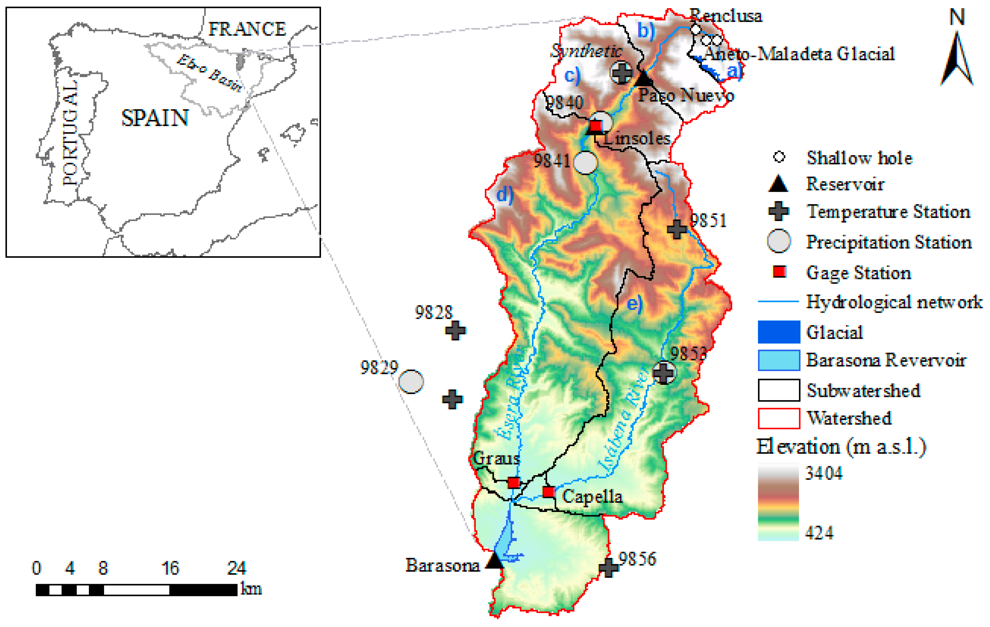
2.1. Study Area

The Barasona reservoir catchment is an agro-forestry region of about 1509 km² located in the Central Spanish Pyrenees (Figure 1). The Barasona reservoir was built in 1932 to supply water for irrigation and power generation. The area is characterized by its abrupt topography, with an average slope of 39%. The altitudinal range extends from 424 m a.s.l. at the catchment outlet to 3404 m a.s.l. (Aneto Peak) at the headwater (Figure 1). The climate is mountainous (wet and cold), with temperature and precipitation gradients observed in both north–south and west–east directions according to the relief, together with the climatic influences of the Atlantic Ocean and Mediterranean Sea. The topographic heterogeneity of the region partially explains the large spatial variability in annual precipitation, which ranges from 500 mm at the outlet to more than 2500 mm on the divides (more than 3000 m a.s.l.) [20]. Additional studies [21] define the precipitation gradient of the region to be around 1000 mm∙km⁻¹ below 2000 m a.s.l., which decreases by almost half (500 mm·km⁻¹) at the divides. Most of the precipitation falls in autumn and spring. The summer is relatively dry (with occasional rainstorms), as is the winter, when snowfalls alternate with long anticyclonic periods. Temperatures are mainly dictated by the altitudinal gradient. For the whole Pyrenean Range, the temperature gradients have been estimated around to be −5 °C∙km⁻¹ of altitudinal increment [20]. The mean annual temperature range from 12 °C at the Barasona reservoir (424 m a.s.l.) to <4 °C in areas above 2000 m a.s.l.

The drainage network is formed by two main rivers, the Ésera River, and its main tributary the Isábena River (Figure 1). Small reservoirs, canals, and dams regulate the Ésera River; whereas, the Isábena River is non-regulated. The Ésera River includes two reservoirs Linsoles and Paso Nuevo (Figure 1), both with a capacity of 3 × 10⁶ m³, which receive a mean annual inflow of 180 × 10⁶ and 101 × 10⁶ m³, respectively. The hydrologic regime of the study area is transitional nival-pluvial characterized by two maxima [20] during the spring period (April–June), due to snowmelt and the late autumn (October–November) due to precipitation. Floods are caused by late spring–early summer snow melts and summer thunderstorms, and heavy rains in late autumn.

There is a well-developed karst system located in the northern area of the catchment (Figure 1). Renclusa, Aigualluts and Toro de Barrancs swallow holes divert the discharge of the upper part of the Ésera River (30 km²), towards the Jueu karst system to the upper Garonne River (Aran Valley, Spain). Comparing specific discharges (period 1963–1994) between the Ésera River headwater and other similar Pyrenean rivers, López-Moreno et al. [22] calculated that 25%–30% of the discharge for the Linsoles catchment was drained to the Garonne River by the karst system. Tracer tests developed by Freixes et al. [23] observed a spring discharge of 0.02–11.5 m³·s⁻¹ for the Jueu karst system and a discharge of 0.02–3 m³·s⁻¹ for the Renclusa swallow hole.

The catchment soils are stony and alkaline with textures ranging from loam to sandy loam. The soils are shallow (<1 m) and, apart from forest soils, have low organic matter contents (<3%–4%). They are generally well drained with limited average water content and moderate to low structural stability. Land use distribution also varies from north to south, with grassland predominating in the highlands, forests in the intermediate ranges, and cultivated land in the more gentle southern areas.

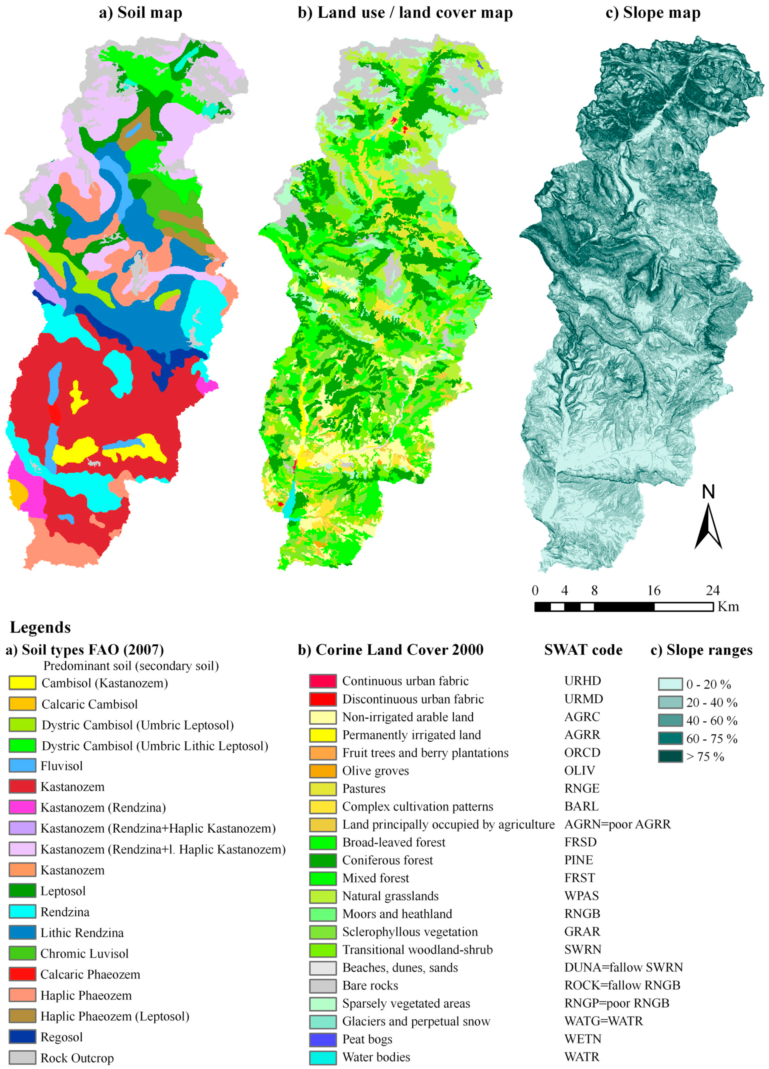
2.2. The SWAT Model and Input Data

SWAT [24] is a physically-based agro-hydrological model, lumped at the subcatchment level, which operates at least on a daily time step, at basin scale. It is designed to predict the impact of management on water, sediment and agricultural chemical yields in ungauged catchments [25]. The input requirements of the model are used to describe the climate, soil properties, topography, vegetation, and land management practices. The hydrologic cycle is climate driven and provides moisture and energy inputs that control the water balance. Flow generation is summed across all of the hydrological response units (HRUs) in a subcatchment, and the resulting flows are then routed through channels, ponds and/or reservoirs to the catchment outlet.

The SWAT model relies on discretization of unique HRUs within each subcatchment that are defined by distinctive combinations of categorized land covers, soil types, and slope, rather than a predefined grid-cell matrix. Since there were few or no tabulated data to characterize the catchment, compiling the input data needed to the model requires considerable research, as well as documenting and adapting the available information. Delineation of the Barasona catchment and its stream network was based on a digital elevation model (DEM) obtained from the Aragón Territorial Information System (SITAR) with a 20 m grid cell resolution (Figure 1). Given the large slope variations in the catchment, five categories of slope were defined to characterize the variety of the surfaces (Figure 2).

Land cover was extracted from the European Project Corine Land Cover map (CLC2000) [26] with a resolution of 100 m. A total of 22 land use classes were present in the catchment and were defined in SWAT by selecting each equivalent class in the SWAT2009 crop database. Five of the SWAT2009 crop classes were edited from the originals by parameterizing their land cover development, in agreement with known regional characteristics to complete the definition of the catchment (Figure 2). The Digital Soil Map of Aragón (Machín J., unpublished data, 2000) was used to define 18 soil types (Figure 2) and a user soil database was developed and incorporated within the ArcSWAT soil database with the required information on the soil types to characterize each soil type. The soil parameters were defined based on field samples (215 samples), literature, mathematical model and field observations. The large percentage of rock outcrop present in the catchment (8.26%) was characterized in both the land cover and soil information layers. As in the case of land cover, rock outcrop was defined by adding a new land cover type called “ROCK” and setting its SCS runoff curve number to 98 (Soil Conservation Service Engineering Division) [27]. In the soil database, it was defined by the “rock outcrop” type of the SWAT2009 database. Finally, the catchment configuration led to 2446 HRUs being defined within ArcSWAT; of which, 50 HRUs were for the Jueu karst system subcatchment, 138 for the Paso Nuevo subcatchment, 191 for the Linsoles subcatchment, 731 for the Capella subcatchment and 748 for the Graus subcatchment.

Daily minimum and maximum temperatures and rainfall data used as climate inputs were based on data for the period from 1 January 1990 to 31 December 2006 (

Table 1. Climatic stations used as inputs in SWAT.

Rainfall Stations	Elevation	Average Annual Precipitation #	Temperature Station	Elevation	Average Annual Temperature #
	m	mm		m	°C
(9829) Mediano	483	750/(679)	(9756) Benabarre	734	11.6
(9840) Eriste	1078	1105/(960)	(9828) Tierrantona	635	12.1
(9841) Sesue	943	1106/(993)	(9829) Mediano	483	12.9
(9853) Serraduy	905	725/(684)	(9853) Serraduy	905	11.9
Synthetic	2000	2232/(1939)	(9851) Las Paules	1402	8.3
			Synthetic	2000	5.0

Notes: ( ) AEMET code station; # Average annual precipitation for periods 1990–2006 and (2003–2005) and temperature for the period 1990–2006.

). Precipitation data were selected from a revised dataset (1955–2006) [28] and temperature data were obtained from the Governmental Meteorological Agency (AEMET). All of the weather stations are in the valley bottoms under the mean elevation of the catchment (Figure 1).

Discharge data for three gauge stations were used to test the accuracy of SWAT simulations (

Table 2. Stream gauge information.

Gauge Station	Elevation	Drainage Area	Streamflow 2003–2005					Streamflow 1994–1996
			m	mdn	sd	max	min	m	mdn	sd	max	min
	m	km2	m3∙s−1					m3∙s−1
Capella	486	428.3	3.7	1.9	3.7	16.6	0.6	5.3	3.4	5.0	24.2	0.6
Linsoles	1050	284.9	6.3	4.7	5.3	20.5	0.7	nd	nd	nd	nd	nd
Graus	455	894.2	18.0	14.2	11.9	47.2	4.8	18.2	14.1	11.2	47.4	4.9

Notes: m: mean; mdn: median; sd: standard deviation; max: maximum; min: minimum; nd: no data.

) (Figure 1). Two of these gauge stations (Graus and Capella) are located on the main stem of the stream system, while the third gauge station is located at the inflow to Linsoles reservoir, near the headwater of the Ésera River. The Linsoles and Graus gauge stations capture the discharge of a 25 km and 85 km stretch of the Ésera River, respectively, and the Capella gauge station captures the discharge of the 61 km stretch of the Isábena River. The Ebro River Basin Authority (Ebro Hydrological Confederation, CHE) provided the river discharge data for the Graus, and Capella gauge stations and Acciona Energía S.A. provided the Linsoles inflow data.

2.3. Model Parameterization

Based on physiographic and land cover similarities within the latitudinal stretch shared by the Isábena and Ésera subcatchments, the results of the automatic calibration process for the natural discharge of the Isábena subcatchment, attempted first in a previous work [19], helped to define the parameters for the whole catchment. Automatic calibration was followed by manual calibration to improve the accuracy of simulated discharges at the existing Capella gauge stations by successive changes in model parameters (

Table 3. SWAT range, default value and final calibrated value of selected SWAT model parameters.

	Parameter	SWAT Range	Default Value	Fitted Value
snow	Snow fall temperature, SFTMP (°C)	−5 to 5	1	1.5
	Snowmelt temperature, SMTMP (°C)	−5 to 5	0.5	4.3
	Maximum melt rate of snow during a year, SMFMX (mm/°C/day)	0–10	4.5	1.5
	Minimum melt rate of snow during a year, SMFMN (mm/°C/day)	0–10	4.5	0.1
	Snow pack temperature lag factor (TIMP)	0–1	1	0.1
	Minimum snow water content at 100% snow cover, SNOCOVMX (mm)	0–500	1	200
	Snow water equivalent at 50% snow cover, SNO50COV	0–1	0.5	0.1
groundwater	Initial depth of water in the shallow aquifer, SHALLST (mm H2O)	100–50,000	0.5	100
	Initial depth of water in the deep aquifer, DEEPST (mm H2O)	1000–50,000	1000	1000
	Groundwater delay, GW_DELAY (days)	0–500	31	31
	Baseflow alpha factor, ALPHA_BF (days)	0–1	0.048	0.02
	Threshold depth of water in the shallow aquifer required for return flow to occur, GWQMN (mm H2O)	0–5000	0	30
	Groundwater “revap” coefficient, GW_REVAP	0.02–0.2	0.02	0.02
	Threshold depth of water in the shallow aquifer for “revap” to occur, REVAPMN (mm H2O)	0–500	1	0
channel	Manning’s “n” roughness value for the main channel, CH_N2	−0.01–0.3	0.014	0.08

). Manual calibration performance was evaluated for each parameter change through visual interpretation of the simulated hydrographs and commonly used statistical measures of agreement between measured and simulated discharges. As no temperature index method or equivalent snow data of the study area were available, defining the snowfall-snowmelt processes in SWAT was an important part of the calibration. Finally, 15 parameters were modified and fixed so as to obtain discharge values that were in good agreement (Table 3). The aforementioned parameterization of the Barasona catchment was performed for the 2003–2005 period, given that it had variable river discharges that provided the variable hydrological conditions to calibrate the SWAT model.

Although studies using SWAT to model sediment and nutrient fluxes typically divide catchments into a larger number of subcatchments, the results of several studies found that SWAT discharge predictions were generally insensitive to variations in subcatchment delineations [3]. Therefore, to assess the ability of the model for discharge simulations at the available gauge stations and to parameterize the headwater reservoirs and the Jueu Karst System the catchment was divided into five representative subcatchments. The downstreamer swallow hole (Renclusa) of the karst system, the reservoirs and the other two gauge stations (Graus and Capella) were used to divide it (Figure 1).

To simulate the loss of discharge by the karst system outside the catchment, SWAT was forced to drain all of the simulated runoff of the headwater subcatchment by the downstream Renclusa swallow hole [29]. The glacial system of Aneto-Maladeta is included in this subcatchment. The inexistence of discharge data from the glacial system leads to its parameterization as an impermeable surface and therefore, the simulated discharge of the swallow hole would be its minimum value.

Reservoir parameterizations for Linsoles and Paso Nuevo reservoirs were based on their technical characteristics (reservoir area, principal and emergency spillways volume) and simulated controlled outflow-target release. The model computes the outflow of the reservoirs as a function of the desired monthly target storage. The target release approach attempts to mimic general release rules used by reservoirs operators. Although the method is simplistic and cannot account for all decision criteria, it can realistically simulate major outflow and low flow periods [30]. Parameterization was based on the management characteristics of the reservoirs. Reservoirs collect water during the high-flow seasons (spring snowmelt and autumn, with maximum flood control is performed, monthly target volumes range 2.2 × 10⁶–3 × 10⁶ m³) and supply water to lowlands during low-flow and high-demand season (summer, monthly target volumes range 1 × 10⁶–1.7 × 10⁶ m³).

2.4. Climatic Scenarios

The highly variable climatic characteristics of the catchment, together with the scarcity and poor distribution of weather data in the area put into question the representativeness of the available climate data, specifically in the case of the headwater. Therefore, the hypothesis was that synthetic climate data and or together with the parameterization of the elevation bands, could better characterize the climate for the alpine headwater enhancing the hydrological simulation. Four scenarios were examined with different input data, (A1), using only the available climate data; (B1), the former plus one synthetic dataset at a higher altitude; (A2), available climate data plus the parameterization of the climate altitudinal gradient; (B2), available and synthetic data plus the same altitudinal gradient. Each scenario was evaluated for the same period as for the calibration (2003–2005) and also for the period (1994–1996) that showed analogous river discharge frequencies which also could serve as validation period.

To account for orographic effects on both precipitation and temperature, SWAT allows up to 10 elevation bands to define the climatic elevation gradient in each subcatchment. Precipitation and maximum and minimum temperatures could be recalculated by SWAT for each band as a function of the respective altitudinal gradients and the difference between the gauge elevation and the average elevation specified for the band [30]. Therefore, 10 homogeneous elevation bands and their estimated altitudinal gradients for the study area were defined in each subcatchment. The altitudinal temperature gradient (TLAPS, temperature lapse rate in SWAT) was set at −5 °C·km⁻¹, as estimated values for the Spanish Pyrenean region (e.g., [20]). The altitudinal precipitation gradient (PLAPS, precipitation lapse rate in SWAT) was set at 1000 mm·km⁻¹ for most of the catchment and was accordingly decreased by subcatchment in relation to the number of elevation bands above 2000 m a.s.l. It is widely documented that the precipitation altitudinal gradient decreases to almost half in the study area at heights above 2000 m. Furthermore, given that the PLAPS could not be defined by elevation band and different surface percentages in the subcatchments are above this altitude, the PLAPS may be undervalued for some subcatchments. Finally, the PLAPS for the subcatchments range from 550 to 1000 mm∙km⁻¹.

Due to the poor distribution of climate stations and the lack of availability of weather data above 1402 m a.s.l. in the catchment, a synthetic daily climate data file was generated for the headwater, which was likely to produce more reliable simulations for high altitude areas. The daily data series (synthetic station) were generated from observed daily data for an intermediate point of the headwater (Figure 1) at an altitude of 2000 m a.s.l., since it is from this altitude that the precipitation altitudinal gradient decreases to almost half. For this purpose, temperature (R_tmp) and precipitation (R_pcp) ratios relating to the estimated altitudinal climatic gradients and the difference in elevations between observed and generated climatic stations were calculated and added to the daily observed data following Equations (1) and (2). In the case of precipitation, the ratio was calculated from the average annual precipitation over a ten-year period (Δ_pcp) and the expected average annual precipitation in relation to the precipitation altitudinal gradient (G_pcp) and the difference altitude between the observed (h_o) and the synthetic data (h_s). Temperature data were obtained from Las Paules station (1402 m a.s.l.) and precipitation data from Eriste station (1072 m a.s.l.), these being the closest stations to the selected point for the synthetic station. The main generated data requirement was to maintain the altitudinal gradients for the region, a precipitation altitudinal gradient of 1000 mm∙km⁻¹ and a temperature altitudinal gradient (G_tmp) of −5 °C∙km⁻¹.

R_tmp = (h_s − h_o) × G_tmp

(1)

R_pcp = (Δ_pcp + (h_s − h_o) × G_pcp)/Δ_pcp

(2)

2.5. Model Evaluation

Model performance was evaluated through visual interpretation of the simulated hydrographs and commonly used statistical measures of agreement between measured and simulated discharge in the gauge stations of Linsoles, Graus, and Capella. The Nash-Sutcliffe model efficiency (NSE) [31], average runoff volume deviation (Dv) and root mean squared error (RMSE) were used for measuring hydrologic model performance. Given that the importance of high flows in mountainous regions, the three statistical measures were also used for river discharges higher than 75% of the observed discharges for the assessed periods (NSE₂₅, Dv₂₅ and RMSE₂₅). These statistics were used to quantitatively assess the ability of the model to replicate temporal monthly trends and high flows in measured data. According to Moriasi et al. [32], a model discharge performance is considered satisfactory if NSE ≥ 0.50 on a monthly time step. During the calibration period, values of NSE > 0.75 are considered to be very good whilst values of NSE ≤ 0.50 are considered unsatisfactory. The Dv values describe the average differences between measured and simulated values. Apart from the Linsoles gauge station that had no data for the validation period, the four scenarios were evaluated in the three gauge stations for the calibration and validation periods.

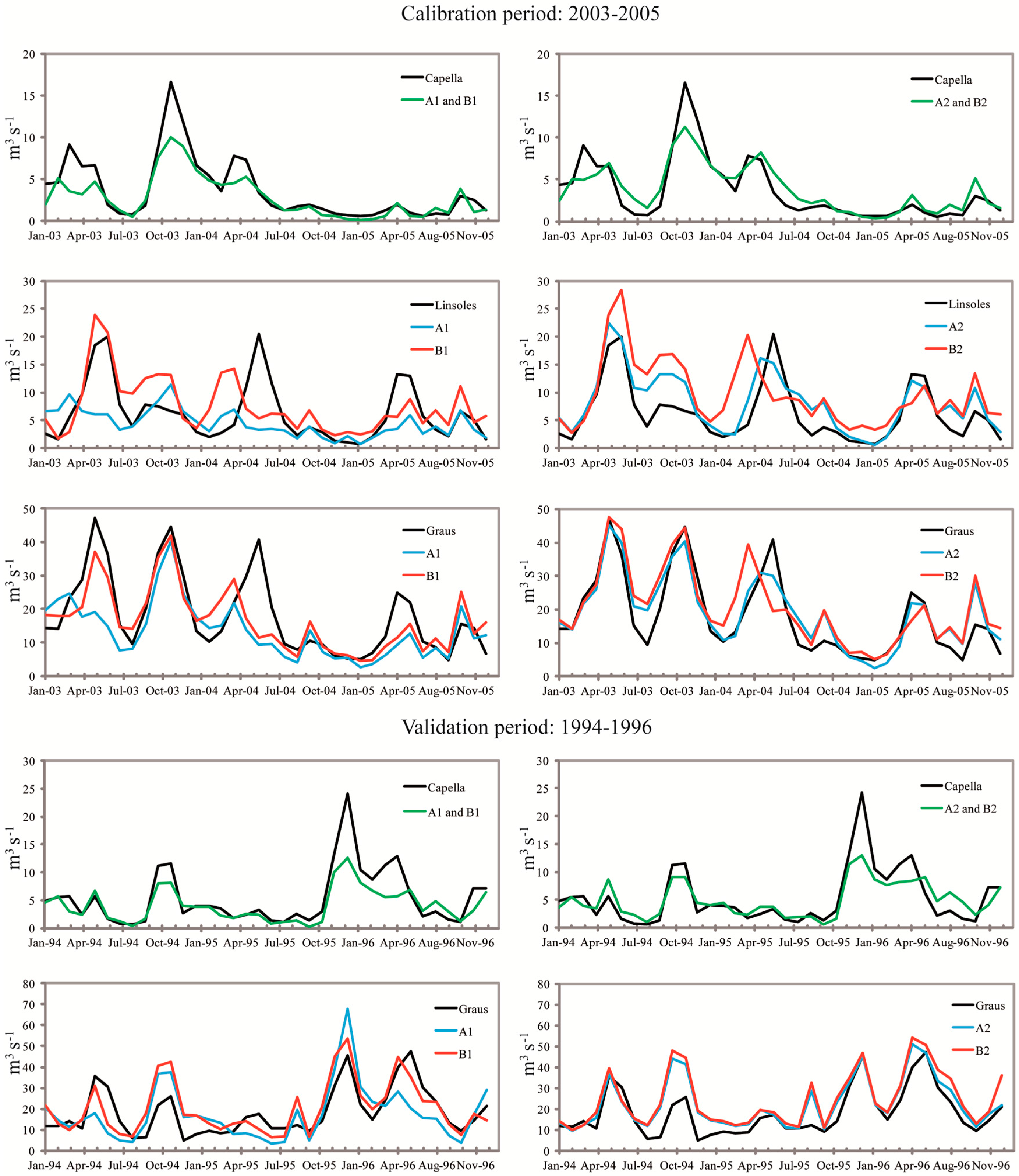
3. Results and Discussion

The SWAT model response for the Barasona catchment, using four different configurations for climate characterization, was compared by means of statistical measures of the simulated river discharges with that observed and the visual interpretation of the simulated hydrographs (

Table 4. Statistical measures of agreement between measured and simulated streamflow for the scenarios A1, B1, A2 and B2 in the gauge stations for the calibration and validation periods.

Scenarios	m	mdn	sd	NSE	Dv	RMSE	NSE25	Dv25	RMSE25
	m3∙s−1				%	m3∙s−1		%	m3∙s−1
2003–2005
Capella
A1	2.8	2.0	2.5	0.73	23.3	1.9	−0.30	20.8	3.6
B1	2.8	2.0	2.5	0.73	23.4	1.9	−0.30	20.8	3.6
A2	3.8	2.9	2.8	0.80	−4.6	1.7	0.35	9.6	2.5
B2	3.8	2.9	2.8	0.80	−4.5	1.7	0.35	9.6	2.5
Linsoles
A1	4.5	3.8	2.5	−0.09	28.5	5.5	−4.45	66.6	10.2
B1	7.6	6.0	5.1	0.13	−20.4	4.9	−1.23	22.1	6.5
A2	8.2	7.3	5.2	0.62	−29.7	3.2	0.49	−2.9	3.1
B2	9.7	8.3	6.0	−0.28	−54.3	5.9	−0.95	−1.5	6.1
Graus
A1	13.5	12.4	8.4	0.28	25.1	9.9	−3.54	44.2	17.5
B1	16.6	15.8	9.3	0.57	8.0	7.7	−1.28	29.2	12.4
A2	19.2	18.4	10.6	0.83	−6.6	4.8	0.66	7.2	4.8
B2	20.8	18.2	11.3	0.62	−15.1	7.2	0.07	8.0	7.9
1994–1996
Capella
A1	4.0	3.1	2.9	0.61	26.6	3.2	0.49	42.0	6.2
B1	4.0	3.1	2.9	0.61	26.6	3.2	0.49	42.2	6.2
A2	5.0	4.0	3.1	0.67	9.2	2.9	0.64	32.4	5.2
B2	5.0	4.1	3.1	0.67	9.2	2.9	0.64	32.5	5.2
Linsoles
A1	nd	nd	nd	nd	nd	nd	nd	nd	Nd
B1	nd	nd	nd	nd	nd	nd	nd	nd	Nd
A2	nd	nd	nd	nd	nd	nd	nd	nd	Nd
B2	nd	nd	nd	nd	nd	nd	nd	nd	Nd
Graus
A1	17.6	15.3	13.0	0.13	3.8	10.5	−5.09	15.1	17.0
B1	20.3	17.0	12.5	0.47	−11.7	8.2	−1.55	0.3	11.0
A2	22.6	18.6	11.9	0.54	−22.1	7.7	−0.32	−4.4	7.9
B2	24.7	19.3	13.0	0.34	−31.1	9.2	−0.92	−11.5	9.6

Notes: m: mean; mdn: median; sd: standard deviation; NSE: Nash-Sutcliffe model efficiency; Dv: average runoff volume deviation; RMSE: root mean squared error; NSE₂₅: Nash-Sutcliffe model efficiency for high flows; DV₂₅: average runoff volume deviation for high flows; RMSE₂₅: root mean squared error for high flows; nd: no data.

and Figure 3). The model performed predictions of subcatchment river discharges, with a variety of NSE, Dv and RMSE values for the different scenarios, gauge stations and periods (Table 4).

Differences between outputs for scenarios A1, B1, A2 and B2 have been found for each subcatchment and for the calibration and validation periods. Scenario A1 corresponded to the result of the calibration process and could be considered as the initial conditions in which the assessed climatic strategies were added. This scenario performed a general underestimation of the river discharges, particularly for the snowmelt period, for all of the gauge stations and periods, yielding statistical measures that were poor for the Linsoles and Graus gauge stations, and acceptable for Capella. As the inclusion of the synthetic station only affected the simulated climatic conditions of the Ésera headwater, the Isábena River subcatchment (Capella gauge) was not influenced by its introduction and its simulated discharge was only affected by the parameterization of the elevation bands for the estimated climate altitudinal gradient. Therefore, the statistical measures for Capella gauge station were equal between A1 and B1 and between A2 and B2. The scenarios which yielded the best statistical measures for the Capella gauge station were A2 and B2, both with the parameterization of the elevation bands. Graus and Linsoles gauge stations for the Ésera River yielded the greatest differences between subcatchments, scenarios and periods. The Ésera headwater at Linsoles gauge station showed the greatest differences because introducing the synthetic station directly affected its subcatchment climate characterization and simulated runoff (scenarios B1 and B2). This synthetic station developed high flows, which compared to scenario A1 improved runoff for Graus and Linsoles gauge stations in B1, but not after adding the elevation bands for scenario B2. Introducing the elevation bands increased the simulated available water and snowfall retention in the catchment, improving the simulated river discharges, and the greatest values of NSE and RMSE for all gauge stations and periods being those of scenario A2. Scenario B2 for Graus and Linsoles gauge station with the synthetic station and the parameterization of the elevation bands resulted in an excess of available water which worsened discharge simulation, especially for Linsoles gauge station. Apart from the high values of Dv observed for Linsoles and Graus gauge stations for the validation period, the statistical measures of the simulated river discharges for all the scenarios, gauge stations and periods indicated that scenario A2 is the strategy that best parameterizes the highly variable climate of the Barasona catchment.

Other authors have reported similar calibration statistics for SWAT model performance in mountain catchments. For example, Fontaine et al. [10] described a monthly NSE of 0.86 with a Dv of −9.8%, Zhang et al. [11] reported a maximum monthly NSE value of 0.85 and Flynn and Van Liew [12] noted a monthly NSE of 0.86.

The dammed characteristics of the Ésera River influence simulation results and detailed daily outflow in Paso Nuevo and Linsoles reservoirs might contribute to a significant improvement in the simulation of Linsoles and Graus gauge stations. The inexistence of outflow data for Paso Nuevo reservoir and the limited information on Linsoles reservoir suggests that the most realistic approach to simulating both reservoirs is their parameterization via the SWAT target volume option. Discordances between simulated and observed high flows of snowmelt river discharge for the Ésera River (Linsoles and Graus gauge stations) could be due to this (annual/monthly homogenized) option of simulation for the reservoirs. For the Ésera headwater, the retention characteristics of the reservoirs were insufficient to accumulate the excess of available water generated in scenarios B1 and B2 (with the synthetic station) to delay the simulated snowmelt high flows (Figure 3).

The simulated karst system performed differently with average monthly discharges from 0.61 to 1.64 m³∙s⁻¹ according to the simulated available water of each scenario for the headwater. Scenario A1 predicted the lowest and B2 the largest amount of discharge with 13%–21% of discharge to the Garonne River for the Linsoles gauge station. Results are in the range of the observations for the Jueu Karst System [22,23].

A detailed subcatchment subdivision and parameterization of the elevation bands is recommended to perform a detailed headwater simulation, given that altitudinal climate gradients in SWAT are defined at subcatchment level. Due to the rugged topography of the headwater the estimated optimal horizontal limit of 2000 m a.s.l., at which the estimated precipitation altitudinal gradient decreases to almost half, would seem to be difficult to achieve. Hence, for areas with complex topography and variable climatic elevation gradients, the elevation band level should have better parameterized the temperature and precipitation altitudinal gradients.

4. Conclusions

Scarce and poorly distributed climatic input data and highly variable climate in mountain regions constitute the main challenges to performing good characterization of the spatial patterns of climatic variables in hydrological models such as SWAT. It was necessary to establish and evaluate strategies for generating synthetic climate data and reproducing the climatic altitudinal gradients in order to overcome these challenges and to better characterize the climatic variables and the hydrological simulations of the Barasona catchment. In this study, the simulated four scenarios with different climatic inputs served to evaluate the strategies by river discharge performance and to identify that the parameterization of elevation bands with the estimated altitudinal gradients and without generated climatic data was the best scenario (A2). Variability in snow accumulation and melt processes and the impact on water balance emphasize the important role played by the parameterization of altitudinal climatic gradients in elevation band strategies in catchments with low-density precipitation and temperature datasets and strong altitudinal climatic gradients. In addition, simulated discharges allowed the influence of the headwater reservoirs and karst system to be evaluated. Other weather data sources, such as radar or satellite, would improve climatic characterization since these data sources could provide better definitions of the spatial climatic variability.

The increase in the water demand for agriculture and the predicted changes in hydrological trends facing water shortages, especially in the Mediterranean region, strengthen the need for assessment, prediction and planning of water resources from mountain headwater catchments that are the suppliers to the agricultural lowlands. These scenarios reinforce the necessity for modelling the availability of water to anticipate water storage in view of drought periods and discharge changes. Therefore, as the Spanish Pyrenean region is a main water source and holds several reservoirs that store water for irrigation of the drier agricultural lowlands, environmental management plans at a regional scale using models such as SWAT afford a perspective that cannot be obtained with other tools and serve as a chief instrument for assisting in the regulation of headwaters such as the Barasona catchment. The success of SWAT evaluation in computing the hydrologic component in this mountainous catchment, as illustrated in this study, provides an opportunity to extend the use of the model to other catchments in the Pyrenean region.

References

1. García-Ruiz, J.M.; López-Moreno, J.I.; Vicente-Serrano, S.M.; Lasanta-Martínez, T.; Beguería, S. Mediterranean water resources in a global change scenario. Earth-Sci. Rev. 2011, 105, 121–139. [Google Scholar] [CrossRef] [Green Version]
2. Krysanova, V.; White, M. Advances in water resources assessment with SWAT—An overview. Hydrol. Sci. J. 2015, 60, 771–783. [Google Scholar] [CrossRef]
3. Gassman, P.W.; Reyes, M.R.; Green, C.H.; Arnold, J.G. The Soil and Water Assessment Tool, Historical development and future research directions. Trans. ASABE 2007, 50, 1211–1250. [Google Scholar] [CrossRef]
4. Stratton, B.T.; Sridhar, V.; Gribb, M.M.; McNamara, J.P.; Narasimhan, B. Modeling the spatially varying water balance processes in a semi-arid mountainous watershed of Idaho. J. Am. Water Resour. Assoc. 2009, 45, 1390–1408. [Google Scholar] [CrossRef]
5. Cao, W.; Bowden, W.B.; Davie, T.; Fenemor, A. Multi-variable and multi-site calibration and validation of SWAT in a large mountainous catchment with high spatial variability. Hydrol. Process. 2006, 20, 1057–1073. [Google Scholar] [CrossRef]
6. Tobin, K.J.; Bennett, M.E. Using SWAT to model streamflow in two river basins with ground and satellite precipitation data. J. Am. Water Resour. Assoc. 2009, 45, 253–271. [Google Scholar] [CrossRef]
7. Masih, I.; Maskey, S.; Uhlenbrook, S.; Smakhtin, V. Assessing the impact of areal precipitation input on streamflow simulations using the SWAT model. J. Am. Water Resour. Assoc. 2011, 47, 179–195. [Google Scholar] [CrossRef]
8. López-Vicente, M.; Navas, A.; Gaspar, L.; Machín, J. Advanced modelling of runoff and soil redistribution for agricultural systems, The SERT model. Agric. Water Manag. 2013, 125, 1–12. [Google Scholar] [CrossRef] [Green Version]
9. Yu, M.; Chen, X.; Li, L.; Bao, A.; de la Paix, M.J. Streamflow simulation by SWAT using different precipitation sources in large arid basins with scarce raingauges. J. Am. Water Resour. Assoc. 2011, 25, 2669–2681. [Google Scholar] [CrossRef]
10. Fontaine, T.A.; Cruickshank, T.S.; Arnold, J.G.; Hotchkiss, R.H. Development of a snowfall-snowmelt routine for mountainous terrain for the soil water assessment tool (SWAT). J. Hydrol. 2002, 262, 209–223. [Google Scholar] [CrossRef]
11. Zhang, X.; Srinivasan, R.; Debele, B.; Hao, F. Runoff simulation of the headwaters of the Yellow River using the SWAT model with three snowmelt algorithms. J. Am. Water Resour. Assoc. 2008, 44, 48–61. [Google Scholar] [CrossRef]
12. Flynn, K.F.; Van Liew, M.W. Evaluation of SWAT for sediment prediction in a mountainous snowmelt-dominated catchment. Trans. ASABE 2011, 54, 113–122. [Google Scholar] [CrossRef]
13. Rahman, K.; Maringanti, C.; Beniston, M.; Widmer, F.; Abbaspour, K.; Lehman, A. Streamflow modeling in a highly managed mountainous glacier watershed using SWAT, the Upper Rhone River watershed case in Switzerland. Water Resour. Manag. 2013, 27, 323–339. [Google Scholar] [CrossRef]
14. Viviroli, D.; Weingartner, R.; Messerli, B. Assessing the hydrological significance of the World’s mountains. Mt. Res. Dev. 2003, 23, 32–40. [Google Scholar] [CrossRef]
15. Valero-Garcés, B.L.; Navas, A.; Machín, J.; Walling, D. Sediment sources and siltation in mountain reservoirs, a case study from the Central Spanish Pyrenees. Geomorphology 1999, 28, 23–41. [Google Scholar] [CrossRef]
16. Navas, A.; Valero-Garcés, B.L.; Gaspar, L.; Machín, J. Reconstructing the history of sediment accumulation in the Yesa reservoir, an approach for management of mountain reservoirs. Lake Reserv. Manag. 2009, 25, 15–27. [Google Scholar] [CrossRef]
17. Navas, A.; Valero-Garcés, B.L.; Gaspar, L.; Palazón, L.; Machín, J. Radionuclides and stable elements in the sediments of the Yesa reservoir (Central Spanish Pyrenees). J. Soils Sediments 2011, 11, 1082–1098. [Google Scholar] [CrossRef] [Green Version]
18. López-Moreno, J.I.; Beniston, M.; García-Ruiz, J.M. Environmental change and water management in the Pyrenees, Facts and future perspectives for Mediterranean mountains. Glob. Planet. Chang. 2008, 61, 300–312. [Google Scholar] [CrossRef]
19. Palazón, L.; Navas, A. Application and validation of SWAT model to an alpine catchment in the Central Spanish Pyrenees. In Proceedings of the 2011 International SWAT Conference, Toledo, Spain, 15–17 June 2011; pp. 162–172.
20. García-Ruiz, J.M.; Beguería, S.; López-Moreno, J.I.; Lorente, A.; Seeger, M. Los Recursos Hídricos Superficiales del Pirineo Aragonés y su Evolución Reciente; Geoforma Ediciones: Logroño, Spain, 2001. [Google Scholar]
21. Rijckborst, H. Hydrology of the upper garonne basin (Valle de Arán, Spain). Leidse Geol. Meded. 1967, 40, 1–74. [Google Scholar]
22. López-Moreno, J.I.; Beguería, S.; García-Ruiz, J.M. El régimen del río Ésera, Pirineo Aragonés, y su tendencia reciente. Bol. Glaciol. Aragon. 2002, 3, 131–162. (In Spanish) [Google Scholar]
23. Freixes, A.; Monterde, M.; Ramoneda, J. Tracer test in the Joèu karstic system (Aran Valley, Central Pyrenees, NE Spain). In Tracer Hydrology 97; Kranjc, A., Ed.; Balkema: Rotterdam, The Netherlands, 1997; pp. 219–225. [Google Scholar]
24. SWAT. Soil and Water Assessment Tool, SWAT Model Software. U.S. Department of Agriculture-Agricultural Research Service, Grassland, Soil & Water Research Laboratory, Temple, Texas. Available online: http://swatmodel.tamu.edu/software/swat-model/ (accessed on 22 June 2011).
25. Arnold, J.G.; Srinivasan, R.; Muttiah, R.S.; Williams, J.R. Large area hydrologic modelling and assessment Part I, Model Development. J. Am. Water Resour. Assoc. 1998, 34, 73–89. [Google Scholar] [CrossRef]
26. CLC2000. Available online: http//www.eea.europa.eu/data-and-maps/data/corine-land-cover-clc2000-100-m-version-12–2009 (accessed on 3 May 2010).
27. Soil Conservation Service Engineering Division. Urban Hydrology for Small Watersheds; U.S. Department of Agriculture: Washington, DC, USA, 1968. [Google Scholar]
28. Vicente-Serrano, S.M.; Beguería, S.; López-Moreno, J.I.; García-Vera, M.A.; Stepanek, P. A complete daily rainfall database for north-east Spain, reconstruction, quality control and homogeneity. Int. J. Climatol. 2009, 30, 1146–1163. [Google Scholar] [CrossRef] [Green Version]
29. Palazón, L.; Navas, A. Evaluation of sediment production of an alpine catchment with SWAT. Z. Geomorphol. 2013, 57, 69–85. [Google Scholar] [CrossRef]
30. Neitsch, S.L.; Arnold, J.G.; Kiniry, J.R.; Williams, J.R. Soil and Water Assessment Tool Theoretical Documentation, Version 2009 USDA. In Soil and Water Research Laboratory; Blackland Research Center: Temple, TX, USA, 2011. [Google Scholar]
31. Nash, J.E.; Sutcliffe, J.V. River flow forecasting through conceptual models, I. A discussion of principles. J. Hydrol. 1970, 10, 282–290. [Google Scholar] [CrossRef]
32. Moriasi, D.N.; Arnold, J.G.; Van Liew, M.W.; Bingner, R.L.; Harmel, R.D.; Veith, T.L. Model evaluation guidelines for systematic quantification of accuracy in watershed simulations. Trans. ASABE 2007, 50, 885–900. [Google Scholar] [CrossRef]
Figure 1. DEM and location of the Barasona catchment in the Ebro Basin (Spain). Situation of the reservoirs, shallow holes, gauge and climatic stations. The boundaries of the five representative subcatchments are also shown: (a) Renclusa shallow hole (Jueu Karst System); (b) Paso Nuevo; (c) Linsoles; (d) Graus and (e) Capella.
Water 08 00471 g001
Figure 2. Distribution of soil types (a), land covers and translation from Corine Land Cover (2000) classifications into SWAT2009 code (b) and slopes (c) in the catchment.
Water 08 00471 g002
Figure 3. Observed and simulated hydrographs for the assessed scenarios A1, B1, A2 and B2 for the Linsoles, Capella and Graus gauge stations and calibration and validation periods.
Water 08 00471 g003