Spatial Distribution and Relationship between Slope Micro-Topography Changes and Soil Aggregate Stability under Rainfall Conditions

Abstract

Natural rainfall affects the stability of soil aggregates by the kinetic energy of the rain changing the morphological characteristics of slope micro-topographic factors. Although the relationship between the stability of soil aggregates and micro-topography is not very significant at the slope scale, there are also rules to be found. This study aims to explore the relationship between slope micro-topography and aggregate stability, and to observe the spatial distribution of aggregate stability after water erosion. In this study, a digital elevation model of slope micro-topography was established by using a three-dimensional laser scanner to observe the slope erosion changes after rainfall events and clarify the spatial changes of soil aggregate stability and its relationship with slope micro-topography by combining geostatistics and generalized additive model (GAM). The results showed that the area of serious water erosion in the lower part of the slope accounted for 38.67% of the slope, and the micro-topography index of the slope changed obviously after rainfall, with the slope increasing by 3.1%, the surface roughness increasing by 5.34%, the surface cutting degree increasing by 26.67%, and the plane curvature decreasing by 61.7%. In addition, the GAM model was used to fit the multivariate variables. The results revealed that the slope and surface roughness were the key factors affecting the stability of water-stable aggregate. The slope and surface roughness were negatively correlated with the stability of water-stable aggregates.

1. Introduction

Soil erosion, which can directly affect the sustainable development of regional environment, is considered one of the most important environmental problems in the world [1,2]. According to the latest global organization data, the global soil erosion induced by water is estimated to be about 20–30 Gt (gigatons) per year [3], Soil erosion directly leads to the loss of nutrient-rich soil particles and aggregates, which makes land degradation and reduce land productivity [4], making it important to study soil erosion caused by water.

In a soil aggregate, there are primary soil particles linked to organic matter, iron oxides, and fungi hypha. As the basic structural unit of soil, soil aggregates play a vital role in almost all processes related to soil erosion [5,6]. Generally speaking, soil aggregates can be divided into macro-aggregates (>0.25 mm) and micro-aggregates (<0.25 mm). Compared with micro aggregates, large aggregates are less easily eroded because of the presence of more organic matter and a higher nutrition level, and generate larger pores for better water seepage and ventilation, and the general aboveground management practice exerts a greater influence on large aggregates than micro-aggregates [7,8]. The stability of soil aggregates is an important soil property, which determines the ability of soil to resist water erosion. It can be quantified by structural stability index (SI), fractal dimension (D), mean weight diameter (MWD), geometric mean diameter (GMD), water-stable aggregates, and normalized stability index [9].

In the process of rainfall, soil aggregates are disintegrated and separated from the soil surface by the impact of raindrops, and finally these dispersed soil aggregates are transported away by surface runoffs [10]. With the occurrence of erosion, the particle size of soil aggregates is changed and redistributed, and moreover, erosion and deposition areas are formed in different soil environments, and the micro-topography is reshaped [11,12]. Other studies have shown that low aggregate stability will aggravate the rapid decomposition of soil aggregates, and the decomposed soil particles will further form surface crusts under the action of rainfall, which will decrease permeability, thus increasing runoffs and soil erosion [13,14]. In addition, a large number of fine particles released after the decomposition of soil aggregates will splash down with raindrops, move away from their original positions and be carried away by runoffs, and moreover, nutrients, pollutants, and even pathogenic microorganisms in the soil may be transported into the water, thus giving rise to agricultural non-point source pollution [15]. Therefore, the study on soil aggregates and their stability is of great significance for maintaining soil productivity and reducing soil erosion and environmental pollution [16].

Soil aggregates and their stability are closely related to surface runoffs and soil erosion. When soil erosion occurs, erosion and deposition areas will be formed on the soil surface, which will change the slope micro-topography (topographic attributes) and soil properties, that is, the stability of soil aggregates [17,18]. Moreover, Jakab G. et al. [19] deemed that the change of aggregate decomposition caused by rainfall can be quantified by repeatedly comparing the digital elevation model (DEM) of the same bare soil surface in theory. However, due to the lack of measurement technology that can be used by previous scholars to obtain accurate information on micro-topographic factors, the research mainly focuses on the evaluation of soil aggregates and their stability in selected topographic positions, but the research on the relationship between slope micro-topography changes and soil aggregates and their stability under water erosion conditions is rarely heard. For example, Zadorova et al. [20] conducted a study on the relationship between the stability of soil aggregates and the selected topography and soil characteristics in the chernozem area of South Moravia using the WSA index. Le Bissonnais et al. [21] investigated the stability of aggregates at five locations along the vertical belt transect in three fields with different soil types. Cantón et al. [22] observed the influence of soil properties and topography on the stability variability of aggregates on the slope of Tabernas, Almeria, Spain. However, the research scope of these scholars is a whole hillside or even a larger scale, and only a specific terrain attribute is selected for research, and the accuracy of DEM data created by them is 1 m, which will undoubtedly produce errors in the results of the study.

To this end, we will use high-resolution (mm-level) 3D laser scanner technology for 3D reconstruction to collect data on soil surface changes during erosion in the experimental site. Therefore, in this study, the 3D laser scanner technology was applied to solve the following scientific problems: (1) How do the micro-topographic factors on the slope scale and the stability of soil aggregates change after water erosion? (2) What is the relationship of the change of micro-topographic factors on slope scale with soil aggregates and their stability?

2. Materials and Methods

2.1. Overview of the Study Area

The study area is located on the slope of the Pisha sandstone area in Baojiagou watershed (110°32′–110°35′ E, 39°46′–39°48′ N) in Zhungeer Banner, Ordos City, Inner Mongolia (Figure 1), with an altitude of 1145–1330 m. The climate is a typical continental monsoon climate, with an average annual temperature of 7.2 °C and an average annual precipitation of 256.4 mm in summer, accounting for 64.1% of the annual precipitation. The frost-free period lasts 100–148 days, and the annual average wind speed is 3.4 m/s. The soil type is mainly chestnut soil, with low organic matter content. The basic physical and chemical properties of the soil are listed in

Table 1. Basic physical and chemical of experimental soil.

Index	Min	Max	Mean
Clay/%	4.87	7.43	5.22
Silt/%	45.83	55.39	51.25
Sand/%	37.18	49.3	43.53
Soil bulk density/(g·cm−3)	1.35	1.7	1.64
STN/(g·kg−1)	0.27	0.56	0.41
Total P/(g·kg−1)	0.98	1.27	1.19
Total K/(g·kg−1)	25.67	37.75	28.89
SOC/(g·kg−1)	1.55	3.72	2.45
Exchangeable cation/(cmol·kg−1)	7.27	9.83	8.26
Soil infiltration rate/(mm/min)	0.6	1.2	0.93

. The soil structure is loose, and the gully density is 5–7 km/km² on average. The soil erosion is serious and natural vegetation is difficult to grow. Since the end of the 20th century, the policy of ecological migration has been implemented in the study area, and the basin is uninhabited at present. The land use types are mainly woodland and grassland, and the vegetation is mainly artificial vegetation for wind resistance, sand fixation and soil and water conservation, including Salix matsudana, Pinus tabuliformis, Platycladus orientalis, Caragana korshinskii, Hippophae rhamnoides, Leymus chinensis, Salsola collina, Heteropappus altaicus, etc.

2.2. Experimental Design and Data Acquisition

This experiment was an in-situ monitoring experiment of natural rainfall in a field runoff plot. Preparation began in June 2020, and the observation time was from June to August in 2020. According to the local actual terrain conditions, a hillside with a slope of 30° was selected, on which all vegetation was cleared. After that, a stainless steel plate of 1 m (length) × 0.5 m (width) was used on the slope, and a runoff plot with a specification of 5 m (length) × 2 m (width) was set, with the plot boundary perpendicular to the contour line, and a leather hammer was used to drive the plate into the ground for 30 cm, with 20 cm left aboveground to block the runoff outside the plot. A water outlet was set at the bottom and equipped with a catchment barrel to collect water and sediment samples (Figure 2). A fixed rainfall monitoring point was set beside the runoff plot, and a siphon rainfall recorder was used to record the atmospheric precipitation process, and a rain gauge was equipped for mutual verification, and the basic data such as rainfall, rainfall intensity, and rainfall duration were measured. During the experiment, a total of 7 erosive rainfalls were observed (

Table 2. Statistical table of rainfall characteristics.

Number	Rainfall Date	Rainfall Duration (min)	Rainfall (mm)	I30 (mm/h)	Rainfall Intensity (mm/h)	Runoff/L	Soil Loss/kg
R1	9 July 2020	180	13.6	4.8	4.53	25	14.8
R2	10 July 2020	244	12	6.6	2.95	10.9	12
R3	12 July 2020	856	32	10.2	2.24	42.9	13
R4	14 July 2020	25	8.4	8.4	20.16	10.9	13
R5	17 July 2020	117	12.4	3.8	6.36	19.8	12.5
R6	12 August 2020	85	10.8	3.2	7.62	14.6	10.4
R7	23 August 2020	263	24.8	6	5.66	8.2	0.22

).

A total of 18 soil sampling points were determined in the runoff plot based on the grid system of 0.8 m (length) × 0.65 m (width), and the soil samples (100 g) of each runoff plot were collected at the soil depth of 0–2 cm with a soil shovel before the first rainfall (9 July 2020). After the last rainfall in the experimental period (24 August 2020), soil samples were collected at the same place once again using the same sampling method as that before the rainfall. The soil samples were sealed with a valve bag, brought back to the laboratory, and air-dried in a natural state to remove coarse roots, small stones, and impurities.

2.3. Establishment and Analysis of Digital Slope Elevation Model

2.3.1. Slope Micro-Relief Model

In this experiment, an RIEGLVZ-400 3D laser scanner made in Austria was used. The instrument acquired 3D point cloud data using the fast-scanning mechanism of a near-infrared laser beam, with a laser emission frequency of 300,000 bit/s, angular resolution of 0.0005°, scanning accuracy (distance of 100 m) of 3 mm (horizontal accuracy) × 2 mm (vertical accuracy), reflectance of 90% within scanning distance of 600 m, vertical scanned area of 0–270°, and horizontal scanned area of 0–360°.

Before the first rainfall, the runoff plot was scanned the first time to obtain the initial point cloud data of the slope. After each rainfall, scanning was performed again after the complete infiltration of water to acquire the morphological development data of the slope. During scanning each time, the 3D laser scanner was fixed on the horizontal ground about 1.5 m away from the slope with a tripod height of 1.10 m to ensure the consistency of each scan. Then, the point cloud coordinates of all scanned point cloud data (186,368 in total) were exported to TXT format by RiSCAN_PRO v1.6.7 software, and loaded into ArcGIS 10.7.0.10450 software to create TIN, and the digital elevation model M-DEM (with an accuracy of 2 mm × 2 mm) of the slope could be obtained by “TIN to raster”. The microstructural change process of experimental plots before and after erosion is shown in Figure 3.

2.3.2. Slope Micro-Topography Analysis and Extraction of Topographic Factors

The change of soil surface microtopography is related to the sediment transport mechanism. In ArcGIS 10.7.0.10450 software, the DEM(Digital Elevation Model) of the slope before rainfall was subtracted by that after rainfall using a raster calculator, and the digital elevation model (M-ΔDEM) of slope micro-topography variation before and after rainfall was established to quantify the change of soil surface micro-topography and distinguish the erosion area (negative difference) from the deposition area (positive difference). Then, reclassification was implemented according to the elevation value, the slope erosion area and deposition area were classified, and the erosion intensity was divided into five levels: slight erosion (0–1 cm), mild erosion (1–2 cm), moderate erosion (2–3 cm), heavy erosion (3–4 cm), and severe erosion (>4 cm).

A total of 4 indexes, namely total erosion area (TEA), total deposition area (TDA), total volume of erosion (TVE), and total volume of deposition (TVD), were selected to analyze the micro-topography changes of the soil surface before and after rainfall, and their overall spatial range was calculated as follows [23]:

$$TEA =n\times A$$

(1)

$$TDA=m\times A$$

(2)

$$TVE={\sum }_{i=0}^{i=n}∆Z_i\times A$$

(3)

$$TVD={\sum }_{j=0}^{i=n}∆Z_j\times A$$

(4)

where: n and m are the number of grid elements with negative and positive DEM differences, respectively; A denotes the grid size; i and j are the grid positions of erosion and deposition, respectively, and ΔZ represents the amplitude of the elevation change.

In addition, 4 micro-topographic factors, namely slope, plane curvature, surface roughness, and surface cutting degree, were selected for further slope micro-topographical analysis [24]. The specific methods and formulas are as follows:

(1)

Slope S

The slope of any point on the surface refers to the angle between the tangent plane passing through the point and the horizontal ground. ArcGIS can be used to extract the slope and quantitatively describe the distribution law of the slope.

(2)

Plane curvature C

Curvature refers to the quantitative measurement factor of the distortion change degree of the topographical surface, which can intuitively reflect the surface relief and can be extracted by using DEM data of a map layer in ArcGIS 10.7.0.10450.

(3)

Surface roughness R

Surface roughness denotes the ratio of the area of a surface unit to its projected area in a certain area:

$$R=1∕\mathit{cos}\left(S\pi ∕180\right)$$

(5)

where S is the slope of the analysis window, (°).

(4)

Surface cutting degree SI

SI is the difference between the mean and minimum value of elevation within the unit:

$$SI=H_{mean}-H_{min}$$

(6)

where: SI represents the surface cutting depth at a certain point within the area, H_mean stands for the average elevation value of the window in the adjacent area, and H_min denotes the lowest elevation value of the window in the adjacent area.

2.4. Analysis of Soil Aggregates

The mechanically stable soil aggregate was determined through the dry sieving method. Specifically, the soil aggregate was sieved into 5 levels—>2 mm (d1), 2–1 mm (d2), 1–0.5 mm (d3), 0.5–0.25 mm (d4), and 0.25–0.1 mm (d5)—using a sieve set, and the soil aggregate particles on the sieve of each level were respectively weighed (accurate to 0.01 g). The water-stable aggregate was determined through the wet sieving method [25]. The aggregate of each particle size determined after dry sieving was proportionally prepared into 50 g of soil samples, which were placed into the sieve set (the mesh size of the sieve set was consistent with that of the dry sieve). Then, the sieve set was put into a settling vat and oscillated up and down at a rate of 30 times/min for 30 min. Finally, the residual particles on each sieve were taken out, dried, and weighed.

Generally, the stability characteristics of aggregates are evaluated using mean weight diameter (MWD) [26], geometric mean diameter (GMD) [27], and soil-stable macro-aggregate content R0.25 [28]. In this study, the damaged percentage content of dry and wet-sieved aggregates was evaluated using the percentage of aggregate damage (PAD) [29], specifically as below:

$$MWD={\sum }_{i=1}^n{X}_i\times W_i$$

(7)

$$GMD=\mathrm{e}\mathrm{x}\mathrm{p}\left\{{\sum }_{i=1}^n\left(m_i\ln X_i\right)/{\sum }_{i=1}^n{m}_i\right\}$$

(8)

$$R_{0.25}=\frac{M_{r>0.25}}{M_T}\times 100\%$$

(9)

$$PAD=\frac{W-W’}{W}\times 100\%$$

(10)

where: n is the number of aggregate size groups; $X_i$ represents the mean diameter of the $i$-th aggregate size component, mm; $W_i$ is the mass fraction of the aggregate with the $i$-th aggregate size, %; $m_i$ is the mass of soil aggregates with different particle sizes, g; $M_r$ denotes the mass of aggregates with different aggregate sizes, g; $M_T$ is the total mass of the aggregate, g; $W \mathrm{and} W’$ are the mass of dry and wet-sieved aggregates with particle sizes of >0.25 mm, respectively.

2.5. Data Processing

The content of soil aggregates with different aggregate sizes in runoff plots before and after rainfall was analyzed via SPSS R26.0.0.0 software in a classical statistical way. Semi-variogram in geostatistics was used to analyze the change of aggregate size distribution and stability of soil aggregates on the slope. This method could estimate the data of unknown sample points according to the known sample points in spatial distribution, and the data were analyzed by semi-variogram using GS+7.0 (Build 25) Professional Edition software (K-S test was performed before analysis, and the data not in a normal distribution were processed through square root transformation). Next, the optimal semi-variogram was chosen and characteristic parameters were acquired, followed by Kriging interpolation to obtain the corresponding spatial distribution map. Afterward, the spatial distribution map was extracted and analyzed using the zonal statistical tool in ArcGIS 10.7 10.7.0.10450 software. Finally, the relationship between slope micro-topographic factors and aggregate stability was observed using the generalized additive model (GAM), with the related calculation formulas as follows:

Semi-variogram [30]:

$$\gamma \left(h\right)=\frac{1}{2N\left(h\right)}{\sum }_{i=1}^{N\left(h\right)}{\left[Z\left(x_i\right)-Z\left(x_i+h\right)\right]}^2$$

(11)

where: $h$ is the separation distance; $N\left(h\right)$ denotes the logarithm of points separated by $h$ on the axis $x$, and $Z\left(x_i\right)$ and $Z\left(x_i+h\right)$ denote the $\left(h\right)$ paired implementation of the observed values $Z\left(x\right)$ and $Z\left(x+h\right)$.

Kriging interpolation method [30]:

$$Z\left(x_0\right)={\sum }_{i=1}^n{\lambda }_{i}Z\left(x_i\right)$$

(12)

where $Z\left(x_0\right)$ and $Z\left(x_i\right)$ are the values of unknown sample points and the values of known points around the unknown sample points, respectively; ${\lambda }_i$ is the weight of the $i$-th known sample point to the unknown sample point; $n$ is the number of known sample points.

GAM [12]:

$$g\left(E\left(Y\right)\right)=\alpha +s_1\left(X_{1i}\right)+s_2\left(X_{2i}\right)+\cdots +s_p\left(X_{pi}\right)$$

(13)

where: g is the connectivity function, E(Y) is the mathematical expected value of the response variable, $\alpha$ is the constant intercept, sp is the nonparametric function of the explanatory variable, and Xpi is the predictive variable. The degree of freedom, statistical values of P and F, determination coefficient R², and variance explained rate are taken as eigenvalues. When the degree of freedom is 1, a linear correlation is observed, and when the degree of freedom is greater than 1, the greater the degree of freedom, the more significant the nonlinear relation. A greater statistical value of F indicates the higher importance of this explanatory factor. A greater coefficient of determination R² represents the better fitting effect, and the explanatory ability of this model for variable relationships is embodied by the variance explained rate.

3. Results

3.1. Slope Micro-Topography Analysis

3.1.1. Slope Erosion and Depositional Characteristics

It could be seen from Figure 4 that the soil erosion intensity was divided into six levels from low to high according to the depth of soil erosion, namely, non-eroded area (deposition area), slight erosion, mild erosion, moderate erosion, heavy erosion, and severe erosion. Combining

Table 3. Changes of digital elevation model after erosion.

Erosion Intensity	Depth/m				Area/m2	Volume/m3
	Min	Max	Mean	STD
Non-eroded	0.000001	0.04	0.033	0.029	4.22	0.14
Slight erosion	0.000008	0.009	0.009	0.006	0.91	0.009
Mild erosion	0.010016	0.019	0.017	0.006	0.86	0.015
Moderate erosion	0.020006	0.029	0.028	0.006	0.62	0.018
Heavy erosion	0.030061	0.039	0.038	0.005	0.21	0.007
Severe erosion	0.040092	0.049	0.044	0.02	0.05	0.002

, it could be observed that the non-eroded area was very large, which was mainly distributed above the slope, accounting for 61.43%, and the average deposition depth was 0.033 m. The intensity of soil erosion was mainly concentrated in slight erosion (0–1 cm) and mild erosion (1–2 cm), and the TEA accounted for 25.75% of the slope, which was concentrated in the lower part of the slope. The TEAs with moderate erosion (2–3 cm) and heavy erosion (3–4 cm) accounted for 9.02% and 3.05% of the slope, respectively, and the TEA with severe erosion of >4 cm only accounted for 0.72% of the slope. For the whole slope, the TVE was 0.14 m³, the TVD was 0.051 m³, and the net soil loss was 0.089 m³, indicating that soil erosion caused by rainfall was very obvious.

3.1.2. Change Features of Topographic Factors

The change characteristics of the micro-topography index before and after the erosion of the whole slope are shown in

Table 4. Changes of micro-topography index before and after erosion.

Topographic Factors	Erosion Phases	Min	Max	Mean	STD
Microslope	Pre-erosion	2.84	82.43	33.83	1.52
	Post-erosion	1.33	82.41	34.88	1.74
Plane curvature	Pre-erosion	−1.265	5.126	0.141	0.008
	Post-erosion	−4.592	6.211	0.054	0.014
Surface roughness	Pre-erosion	1.0004	5.031	1.216	0.193
	Post-erosion	1.0003	7.573	1.281	0.463
Surface cutting degree	Pre-erosion	0.000	0.131	0.015	0.006
	Post-erosion	0.000	0.194	0.019	0.004

. The plane curvature was reduced by 61.7% compared with that before water erosion. The plane curvature can quantify the change degree of surface distortion, which can affect the flow velocity, convergence, and dispersion process of slope runoffs, thus affecting the micro-topography erosion and deposition of the slope. The reduction of this index indicated that the whole slope was eroded in general. The slope was increased by 3.1% compared with that before water erosion. The slope represents the steepness of the surface unit. The increase of this factor manifested that the included angle between the slope and the horizontal ground became larger, that is, the position at the foot of the slope was seriously eroded, which corresponded to the position of the erosion area in Figure 4. The surface roughness and surface cutting degree reflect the fluctuation of the surface and the morphological changes of micro-topography during the erosion process, which were increased by 5.34% and 26.67%, respectively, in comparison with those before water erosion.

Through further detailed observation (

Table 5. Changes of micro-topography index under different erosion intensities before and after erosion.

Erosion Intensity	Microslope		Plane Curvature		Surface Roughness		Surface Cutting Degree
	Pre-Erosion	Post-Erosion	Pre-Erosion	Post-Erosion	Pre-Erosion	Post-Erosion	Pre-Erosion	Post-Erosion
Non-eroded	31.14	33.68	−0.308	0.333	1.182	1.274	0.014	0.018
Slight erosion	32.76	34.59	0.414	0.084	1.225	1.239	0.015	0.017
Mild erosion	34.22	36.16	0.0634	0.038	1.231	1.265	0.016	0.018
Moderate erosion	37.59	38.39	1.073	−1.285	1.294	1.318	0.018	0.020
Heavy erosion	39.25	41.00	3.836	−3.915	1.343	1.376	0.019	0.022
Severe erosion	47.75	48.23	4.084	−2.549	1.578	1.613	0.027	0.026

), the slope kept increasing under the 6 erosion intensities, and the maximum increase in the non-eroded area was 8.15%. The plane curvature could be positive or negative. When it was positive, the pixel bulged, and if it was negative, the pixel concaved. In the non-eroded area, the plane curvature was turned from −0.308 to 0.333, indicating that the surface was transformed from a concave shape into a convex shape after rainfall and sediments were deposited here. The plane curvatures in the slight erosion and mild erosion areas were also reduced to different degrees, reflecting that the two areas were eroded. The plane curvatures in the mild erosion, heavy erosion, and severe erosion areas were turned from positive values into negative values, the erosion degree was more evident, and the slope was changed from a convex slope into a concave slope. It could be seen from Table 2 that as the number of rainfalls increased, there were an increasing number of bulges and depressions on the slope due to raindrop splashing and runoff scouring. The surface roughness values in the areas under the 6 erosion intensities all increased after rainfall, accompanied by an increasing surface depression detention. The surface cutting degrees in the 6 areas changed little.

3.2. Soil Aggregates

3.2.1. Particle Size Distribution Characteristics of Soil Aggregates

It could be seen from Figure 5A that the aggregate size distribution of soil mechanically stable aggregates was normal before rainfall, and the peak value was 1–0.5 mm. After rainfall, the particle size distribution of mechanically stable soil aggregates was approximately normal, without significant difference of other particle sizes except 0.25–0.1 mm from those before rainfall. The particle size of 1–0.5 mm decreased by 0.73% and that of 0.5–0.25 mm decreased by 2.5%. Aggregates with particle sizes of >2 mm and 2–1 mm increased by 6.89% and 4.04%, indicating that mechanically stable soil aggregates changed from a small particle size to a large particle size after rainfall. This is because the slope contains clay minerals such as montmorillonite and kaolinite, which have strong plasticity and adhesiveness after wetting, and there is interaction between clay minerals and organic matter (SOM), and clay mineral aggregates pass through SOM [31]. Moreover, the clay content is very low (Table 1) and the relative increase of sand fraction on the account of decrease of clay fraction in the aggregates.

It could be seen from Figure 5B that only the particle size of 0.25–0.1 mm of water-stable soil aggregates displayed significant differences before and after rainfall, indicating that the water-stable aggregate with the aggregate size of 0.25–0.1 mm was an advantaged particle size, and the content was 21.07–21.93%, followed by the particle size of 0.25–0.1 mm. After rainfall, however, the water-stable aggregates with different particle sizes were reduced compared with those before rainfall, during which the external force contributed a lot to the decomposition of soil aggregates [32]. Compared with mechanically stable aggregates, the content of water-stable aggregates decreased very significantly, and the particle size distribution obviously shifted to a small size, manifesting that although mechanically stable aggregates formed large aggregates after rainfall, their water-stable aggregate content was extremely low, with weak water erosion resistance.

3.2.2. Stability Characteristics of Soil Aggregates

After seven intermittent rainfalls, the indexes (

Table 6. Stability characteristics of soil aggregates before and after erosion.

Sampling Time	MWD		GMD		R0.25		PAD
	Dry Sieving Method	Wet Sieving Method	Dry Sieving Method	Wet Sieving Method	Dry Sieving Method	Wet Sieving Method
Pre-erosion	0.88 ± 0.17 b	0.35 ± 0.11 gh	0.72 ± 0.14 c	0.44 ± 0.07 ef	0.85 ± 0.05 b	0.41 ± 0.09 fg	50.45 ± 3.04 e
Post-erosion	1.05 ± 0.16 a	0.29 ± 0.07 h	0.88 ± 0.15 b	0.42 ± 0.07 fg	0.93 ± 0.04 b	0.38 ± 0.07 fg	58.39 ± 2.11 d

Note: Different letters in the same column represent significant differences.

) of soil aggregate stability were calculated. The MWD and GMD of soil aggregates could reflect the size distribution of aggregates. The larger the value, the higher the degree of aggregation and the better the stability. For mechanically stable aggregates, the MWD after rainfall was higher than that before rainfall at a certain significance level. The MWD of water-stable aggregates was lower than that before rainfall, but no significant difference was observed. The law of GMD data was consistent with the law of MWD. R_0.25 characterized large aggregates in soil, and the larger the value, the more stable the soil aggregates were. The R_0.25 value of mechanically stable aggregates increased by 8% compared with that before rain, and the content was as high as 0.85 and 0.93 before and after rainfall, respectively, that is, the content of large aggregates was high and the mechanical stability was good, but the R_0.25 value of water-stable aggregates was significantly lower than that of mechanical aggregates and lower than that before rainfall. PAD indicated the damage degree of water-stable soil aggregates, and the smaller the PAD, the higher the stability of aggregates. PAD after rainfall increased by 7.94% compared with that before rainfall, and its stability decreased. Therefore, considering several indexes, the reason why the indexes of mechanically stable aggregates are high is that the aggregate structure contains a large number of non-water-stable aggregates, which will be decomposed when meeting water, which cannot accurately explain the quality difference of soil aggregates. Hence, it is more convincing to evaluate the actual situation of soil aggregates with the indexes of water-stable aggregates.

3.2.3. Stability Parameters of Soil Aggregates and Its Spatial Structure Characteristics

The spatial structural characteristics of soil aggregate stability parameters before and after rainfall were analyzed by geostatistics method, as shown in

Table 7. Semi-variogram model of soil aggregate stability parameters and relevant parameters.

Sampling Stage	Soil AGGREGATE Types	Aggregate Stability Parameters	Model	Nugget (m)	Sill (m)	Nugget/Sill (%)	Range (m)	R2	RSS
Pre-erosion	Mechanical stability aggregate	MWD	Spherical	0.00178	0.03106	5.73%	1.36	0.762	0.00001162
		GMD	Spherical	0.00118	0.02286	5.16%	1.32	0.667	0.00003178
	Water-stable aggregate	MWD	Linear	0.002039	0.015016	13.58%	2.74	0.772	0.00000340
		GMD	Spherical	0.00024	0.00627	3.83%	1.03	0.661	0.00000104
Post-erosion	Mechanical stability aggregate	MWD	Linear	0.0284	0.27536	10.31%	2.74	0.531	0.00010070
		GMD	Linear	0.002671	0.02982	8.96%	2.74	0.532	0.00007038
	Water-stable aggregate	MWD	Gaussian	0.00338	0.02685	12.59%	4.48	0.855	0.00000851
		GMD	Gaussian	0.0005	0.00581	8.61%	0.29	0.535	0.00000770

. The optimal models of MWD and GMD parameters of mechanically stable aggregates were spherical models before rainfall and linear models after rainfall. Before rainfall, the MWD of water-stable aggregates was a linear model, GMD was a spherical model, and both were Gaussian models after rainfall. Nugget and RSS of soil aggregate stability before and after rainfall were small and R² was high, indicating that the random variation caused by sampling in the experiment was small, which was mainly controlled by internal factors such as parent material, topographic attributes, and soil types, which was consistent with the research results of [33]. And the fit effect of each parameter and semi-variogram was good, which could well reflect the spatial variation characteristics of each parameter. Sill represented the total variability of variables in space, and the Sill value of aggregate stability changed little before and after rainfall. Nugget/Sill/% stood for the variation characteristics between samples, and all the values were less than 25%, indicating that the variables presented strong spatial autocorrelations. Range was always small, that is, the distance of spatial autocorrelation of each parameter was small.

In this study, based on the semi-variogram model analysis, the spatial distribution map of soil aggregate stability parameters was drawn by Kriging interpolation method (Figure 6). The spatial distribution of MWD and GMD of mechanically stable aggregates before rainfall (Figure 6A) was basically the same. The red high-value area was distributed in the northwest of the slope, and the blue low-value area was distributed in the lower part of the slope, showing an aggregated distribution. After rainfall, the spatial distributions of MWD and GMD of mechanically stable aggregates (Figure 6C) were all banded, and the original red high-value areas became blue low-value areas. Before rainfall, the spatial distribution of MWD and GMD of water-stable aggregates (Figure 6B) was quite different from that of mechanically stable aggregates. The red high-value area of MWD was mainly distributed in the southeast of the slope, and the red high-value area of GMD was in the northeast of the slope. After rainfall, the red high-value area of MWD shifted, and a new red high-value area was formed in the northern part of the slope, and the bottom of the slope changed from a high value to a low value, showing an island-like distribution as a whole, and GMD also showed a similar law.

4. Discussion

4.1. Influence of Rainfall on Slope Micro-Geomorphology Change

The interaction between rainfall and slope soil leads to the change of slope micro-topography. In this study, the middle and lower part of the whole slope was eroded, which might be ascribed to the fact that dry soil was easily stripped and transported at the beginning of rainfall, and deposition occurred at the top of the slope. On the one hand, due to the short slope length and small catchment area on the upper slope, it was difficult to form a concentrated stream, and the runoff energy on the slope was low, so sediments were easily silted up during transport. On the other hand, with the continuous rainfall, the soil was hardened, the soil erodibility was weakened, and the slope runoff energy was not enough to peel off the soil particles at the top of the slope. Therefore, rills first appeared in the middle and lower part of the slope, which was beneficial to their development. With the development of rainfall, rills continued to extend along the slope, widened, and developed deeper through merger and bifurcation, so serious erosion occurred in the middle and lower part of the slope (Figure 4). The correlation between topographic factors and rainfall characteristics under natural rainfall showed (

Table 8. Correlation coefficients between rainfall characteristics and micro-topographic factors.

	Rainfall Duration	Rainfall	I30	Rainfall Intensity	Micro-Slope	Plane Curvature	Surface Roughness	Surface Cutting Degree
Rainfall duration	1
Rainfall	0.897 **	1
I30	0.675	0.548	1
Rainfall intensity	−0.559	−0.528	0.128	1
Micro-slope	−0.065	0.187	−0.463	−0.258	1
Plane curvature	0.459	0.161	0.281	−0.191	0.167	1
Surface roughness	0.081	0.337	−0.383	−0.412	0.949 **	0.127	1
Surface cutting degree	−0.337	−0.248	−0.108	0.247	0.551	0.24	0.512	1

Note: ** The correlation is significant at the level of 0.01 (two-tailed).

) that the rainfall duration was negatively correlated with the micro-slope and surface cutting degree, and positively correlated with the curvature and surface roughness. No significant correlation was observed between rainfall and four topographic factors. I₃₀ was only positively correlated with the curvature, but negatively correlated with the other three topographic factors. The rainfall intensity was only positively correlated with the surface cutting degree.

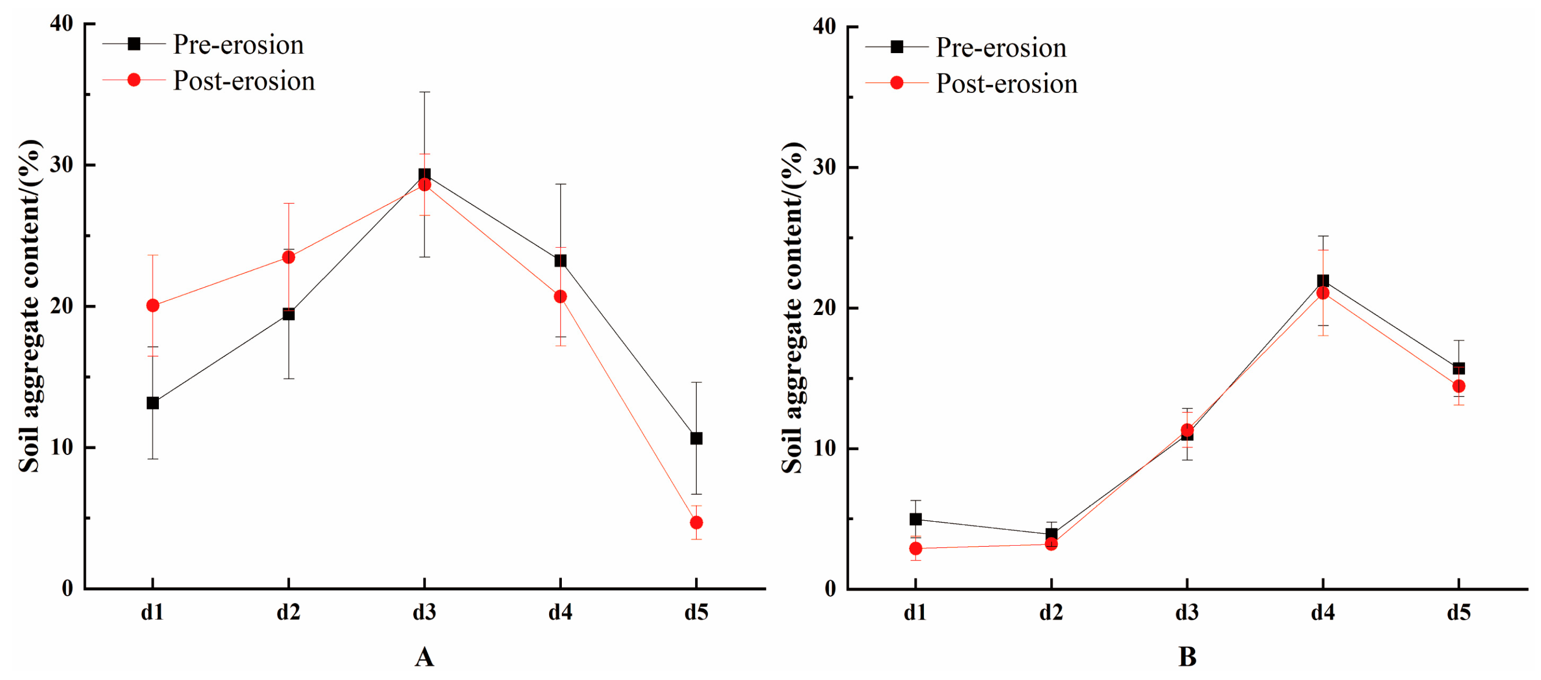
4.2. Rainfall Effects on Soil Aggregates Stability

After the rainfall for more than one month, the stability of water-stable aggregates was lower than that before the rainfall, and Shi et al. [34] thought that the stability of soil aggregates will not be improved again after the drying process, which was also confirmed in this study. Among the seven natural rainfalls, every two rainfalls were spaced by several days, and the aggregates would be fully exposed to the sun and dried. The final result showed that the stability of aggregates was lower than that before the rainfall (Table 6). Dimoyiannis et al. [35] proved through continuous monitoring for two years that among many factors, rainfall and air temperature can strongly affect the dynamic change of soil aggregate stability, which is ultimately ascribed to the dynamic change of soil moisture in the final analysis. He et al. [36] also showed that the dynamic change of MWD with time is negatively correlated with the dynamic change of soil moisture, and the change in the MWD value of water-stable aggregates in this study also follows this law. With the repeated rainfall, soil aggregates are frequently in wetted-dry-wetted cycles, and their stability finally declines. The spatial change of soil aggregate stability, an index used to evaluate the damage of aggregate resistance against external forces to the aggregate [37], on the slope may result from the spatial heterogeneity of soil particles induced by water erosion. Soil particles are redistributed along the slope after being splashed by raindrops and washed by runoffs, thus changing the soil properties at different positions on the slope. In the research of Zhang et al. [38], it was found that the relative content of clay in the surface layer of the slope increased along the runoff direction, but the deformation and destruction of the slope led to the decrease in the relative content of clay in sediments located at the lower part of the slope. Clay particles have large specific surface area and strong cation exchange ability, which can effectively gather stable aggregates [39], and their reduction will inevitably weaken the stability of aggregates at the lower part of the slope.

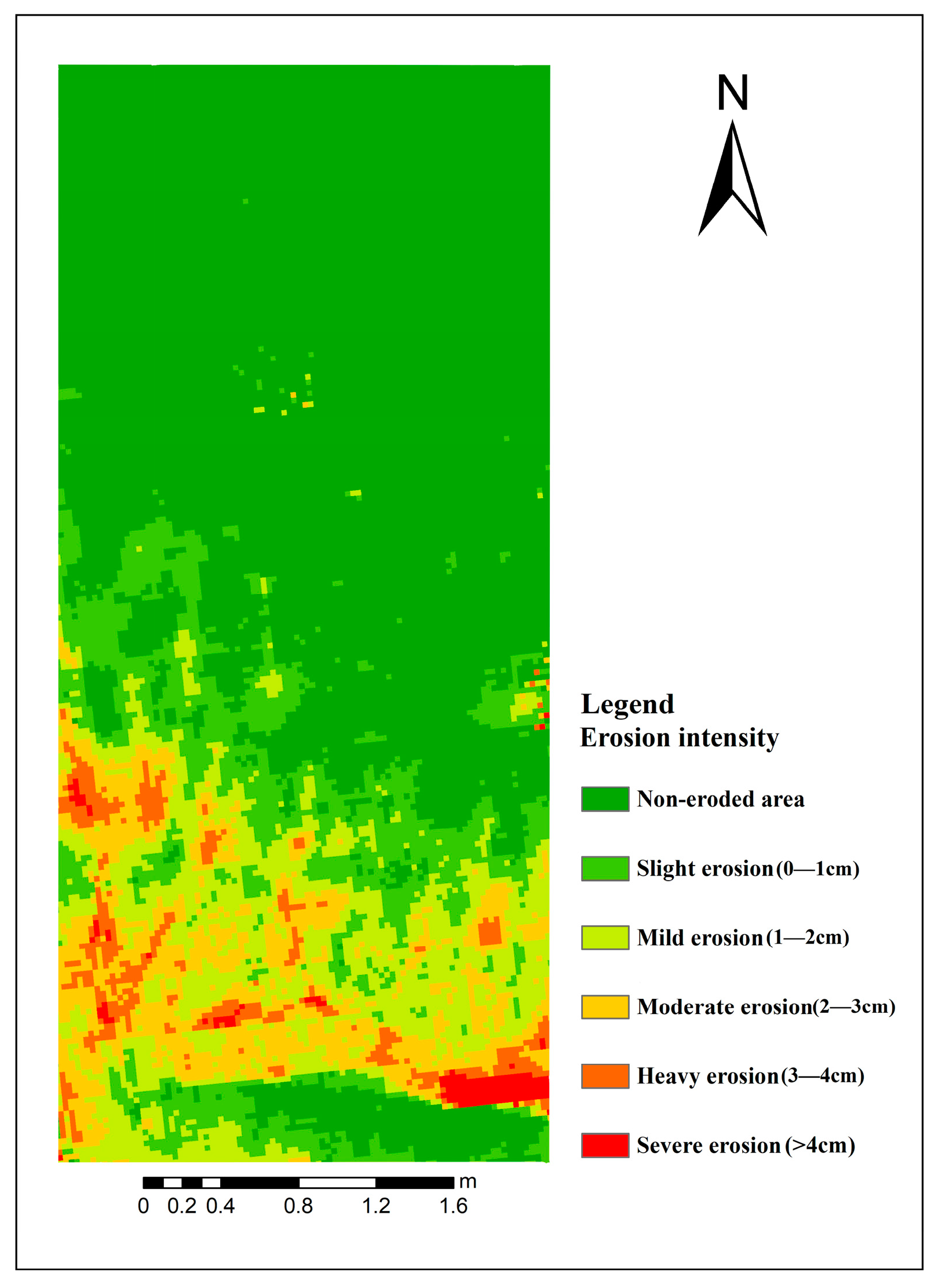
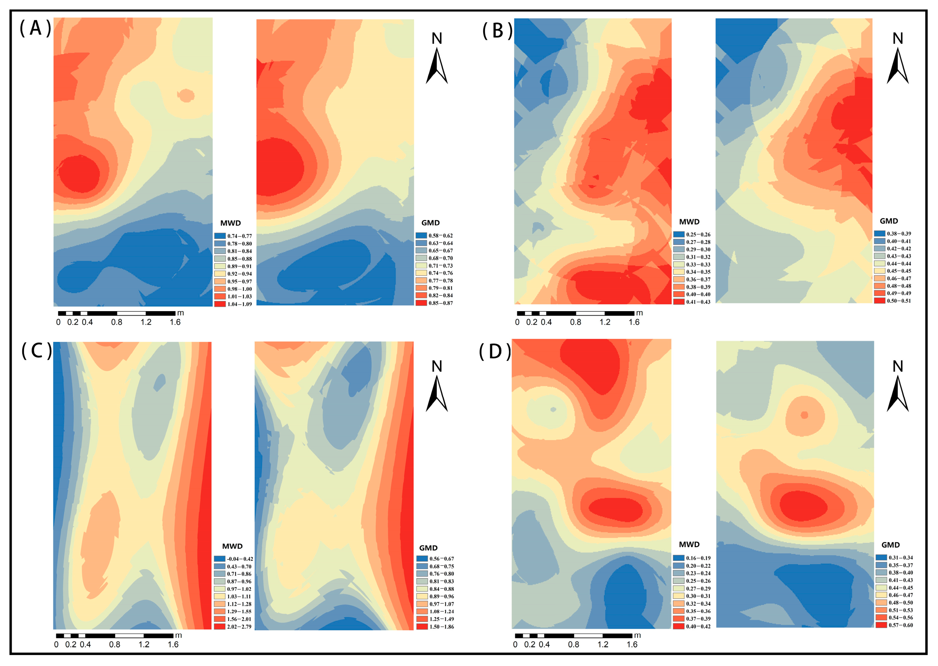
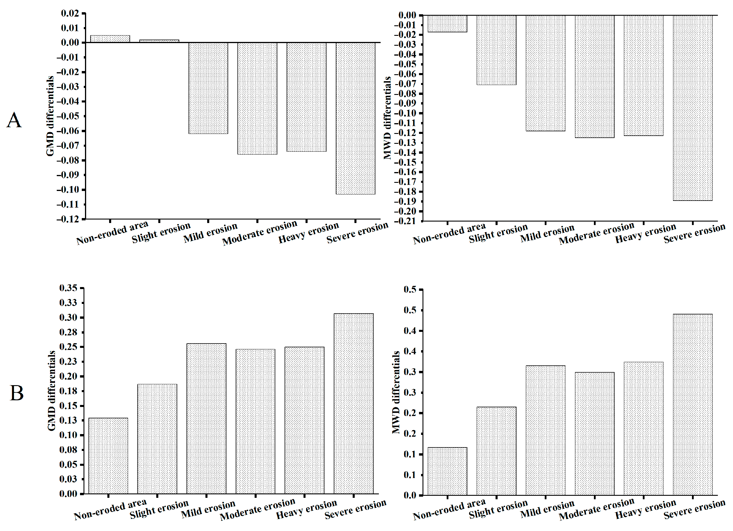
As shown in Figure 7, the difference values of aggregate stability parameters before and after rainfall under various erosion intensities could be observed. The GMD of water-stable aggregates increased by 0.005 and 0.002 in the non-eroded area and slightly eroded area, respectively, which could be regarded as unchanged compared with that before rainfall, and decreased significantly under other erosion intensities. The maximum value of MWD of water-stable aggregates was 0.433, and the minimum value was 0.16, which decreased significantly under all erosion intensities. With the increase of erosion intensity, the MWD decreased by 0.017, 0.071, 0.118, 0.125, 0.123, and 0.189, respectively, which was the same as that studied by Xia et al. [40]. This may be because the aggregate is decomposed by the rainfall into differently sized particles, which block soil pores and form crusts, thus increasing surface runoffs [41], and the more severely eroded areas are more seriously scoured. As shown in Table 6, the PAD after rainfall was higher than that before rainfall, meaning that soil aggregates were easily dispersed when encountering rainfall or runoffs, thus reducing the stability of soil aggregates. The parameters of mechanically stable aggregates increased under different erosion intensities. Teh, C. B. S. [10] pointed out that the stability of soil aggregates depends on the size of individual aggregates. In Table 6, the large aggregates on the whole slope after rainfall were higher than those before rainfall, so the parameters of mechanically stable aggregates would increase under different erosion intensities. Based on the changes in parameters of mechanically stable aggregates and water-stable aggregates under different erosion intensities, it could be found that with the increase of erosion intensity, the stability parameters of aggregates changed extremely obviously, especially under the severe erosion intensity.

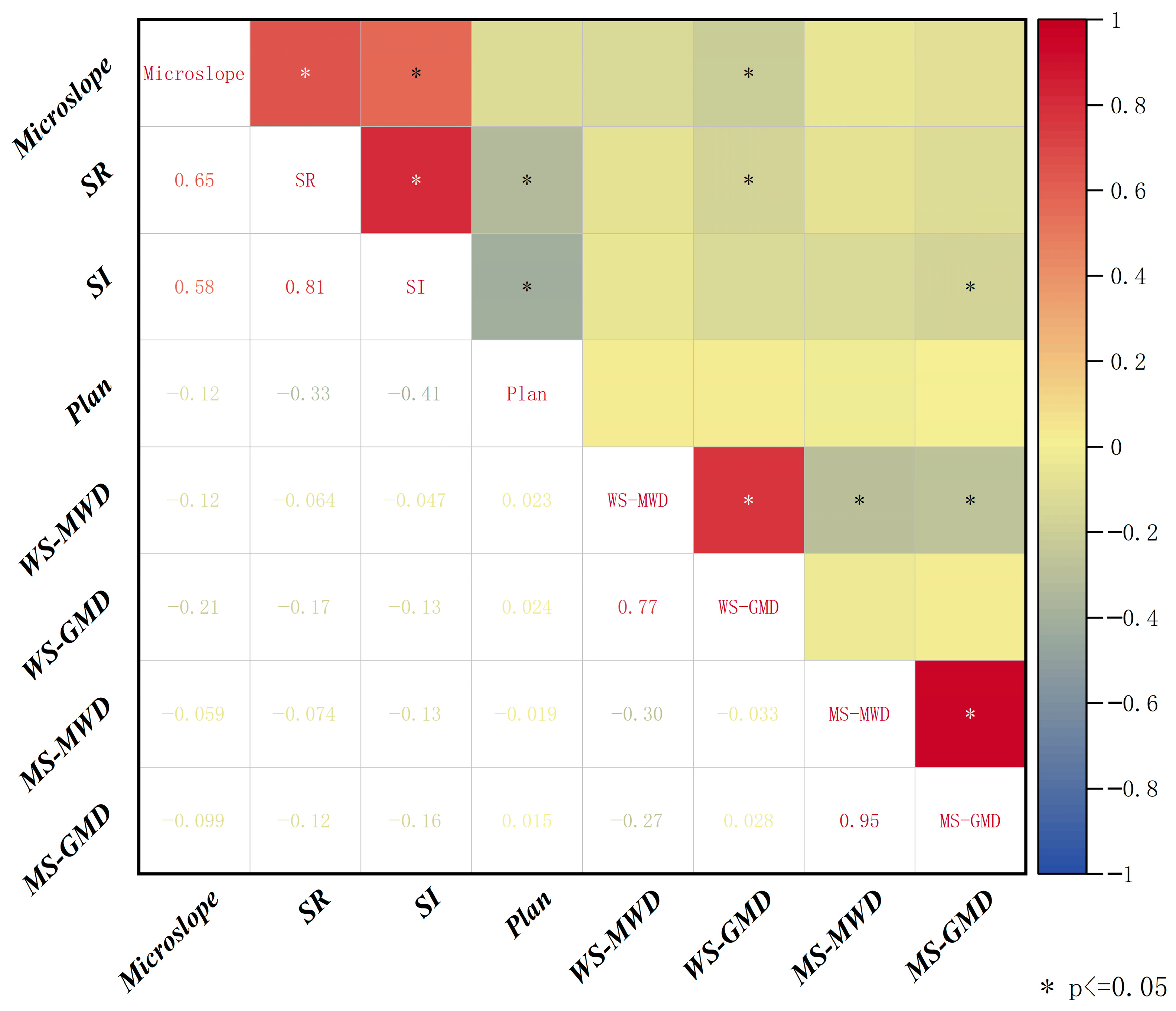
4.3. Relationship between Micro-Topographic Factors and Soil Aggregate Stability

The correlation between micro-topographic factors and stability parameters of soil aggregates was analyzed, and the results are shown in Figure 8. The micro-topographic factors were all correlated with the stability parameters of soil aggregates. The slope was significantly negatively correlated with water-stable GMD (p < 0.05) with a correlation coefficient of −0.21, and presented significant positive correlations with the surface roughness and the surface cutting degree (p < 0.05), with correlation coefficients of 0.65 and 0.58, respectively. The surface roughness showed a significant positive correlation with the surface cutting degree (p < 0.05) and a significant negative correlation with the plane curvature (p < 0.05), with correlation coefficients of 0.81 and −0.33, respectively, and a significant negative correlation with water-stable GMD with a correlation coefficient of −0.17 (p < 0.05). The surface cutting degree was significantly negatively correlated with the plane curvature and mechanically stable GMD (p < 0.05), and the correlation coefficients were −0.41 and −0.16, respectively. The water-stable MWD showed a significant negative correlation with water-stable GMD (p < 0.05), and it was significantly negatively correlated with both mechanically stable MWD and GMD (p < 0.05). There was a significant positive correlation between mechanically stable MWD and mechanically stable GMD (p < 0.05), and the correlation coefficient was 0.95.

According to correlation results between soil aggregate stability parameters and topographic factors in Figure 8, it was found that every two parameters between micro-topographic factors and soil aggregate stability parameters were correlated but insignificantly. Hence, there might be a relationship between micro-topographic factors and soil stability parameters that cannot be explained by a single factor, and linear relationship and nonlinear relationship might exist at the same time. GAM was used to fit the relationship between topographic factors and soil stability parameters. Four soil aggregate stability parameters (water-stable aggregate MWD, water-stable aggregate GMD, mechanically stable aggregate MWD, and mechanically stable aggregate GMD) were used as response variables and four micro-topographic factors (slope, surface roughness, surface cutting degree, and plane curvature) were used to construct models, respectively, for multi-factor fitting (

Table 9. Hypothesis testing results based on GAM.

Response Variable	Influencing Factor	Estimated Value	Degree of Freedom	F Statistic	P	R2
WS-MWD	Micro-slope	2.053	2.628	1.258	0.211	0.481
	Surface roughness	1.000	1.000	0.829	0.364
	Surface cutting degree	2.160	2.775	0.652	0.505
	Plane curvature	1.000	1.000	0.096	0.757
WS-GMD	Micro-slope	3.229	4.064	3.875	0.004	0.519
	Surface roughness	1.000	1.000	5.958	0.015
	Surface cutting degree	2.577	3.305	1.815	0.139
	Plane curvature	1.000	1.000	1.362	0.245
MS-MWD	Micro-slope	1.000	1.000	0.022	0.882	0.378
	Surface roughness	1.000	1.000	0.041	0.840
	Surface cutting degree	1.000	1.000	0.831	0.363
	Plane curvature	2.663	3.270	2.086	0.103
MS-GMD	Micro-slope	1.000	1.000	0.007	0.933	0.401
	Surface roughness	1.000	1.000	0.014	0.905
	Surface cutting degree	1.000	1.000	0.291	0.591
	Plane curvature	3.112	3.815	2.034	0.106

). The results showed that the variance explained rate R² of the model fitting value to the response variable was 0.378–0.519, and the fitting result was of certain reference significance.

For water-stable aggregate MWD, the response variable was nonlinearly related to the slope and surface cutting degree, and linearly related to the surface roughness and plane curvature, among which the slope was the most important influencing factor. The water-stable aggregate GMD was also nonlinearly correlated with the slope and surface cutting degree, and linearly correlated with the surface roughness and plane curvature, but it was influenced by the surface roughness most intensely, and then by the slope. The mechanically stable aggregate MWD and the mechanically stable aggregate GMD were both nonlinearly related to the plane curvature and linearly related to other topographic factors, and the plane curvature was the biggest influencing factor.

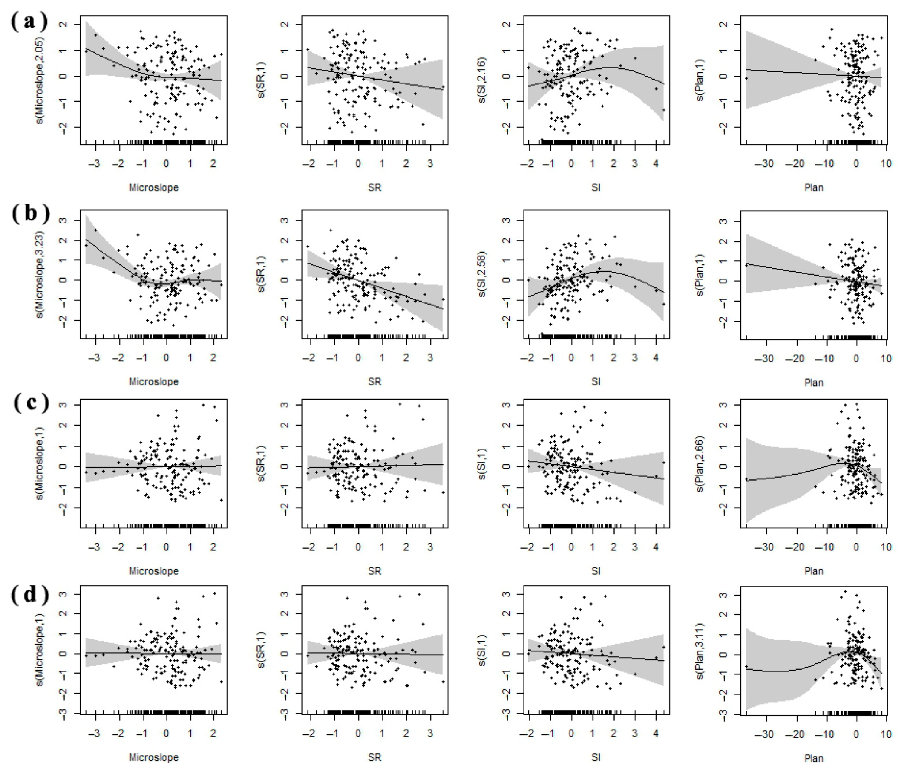
Because the relationship between variables is nonparametric in GAM and cannot be described by simple mathematical formulas, the graphical smooth curve is a common way to observe the dependence between variables in GAM (Figure 9). It could be seen from Figure 9a,b that both MWD and GMD of water-stable aggregates would decrease with the increase of slope, and the relationship between GMD and slope was extremely significant (p < 0.01), which might be attributed to the fact that the erosion and loss of surface soil increased with the increase of slope [42], which led to the increase of runoff velocity, the enhanced scouring of aggregates, the increase of fragmentation rate, and the decrease of aggregation degree. Both MWD and GMD of water-stable aggregates would decrease with the increase of surface roughness, and the relationship between GMD and surface roughness was significant (p < 0.05). Decomposition of soil surface aggregates not only results from the external force of external rainfall and runoffs but also from the wetting process of expansion and explosion caused by the difference between air entrained in aggregates and atmospheric pressure [43]. Generally, the increase of surface roughness will reduce the flow velocity, increase the surface water storage capacity, and enhance infiltration [44], which accelerates the wetting process of aggregates, leading to accelerated decomposition of aggregates and their decreased stability. Figure 9b shows the relationship between the surface roughness and the stability parameters of soil aggregates. The change of the surface roughness value was significantly correlated with the MWD of water-stable aggregates and the MWD of mechanically stable aggregates (p < 0.01). The changes in MWD and GMD of water-stable aggregates first increased and then decreased with the increase in the surface cutting degree, meaning that the stability of water-stable aggregates was high at the subsidence and weak at the uplift. The changes in MWD and GMD of water-stable aggregates also showed the same characteristics with the plane curvature, and the stability of aggregates was negatively correlated with the plane curvature, which was also reflected in the study of Nimmod et al. [45]. This is because organic carbon can be more easily accumulated in the concave surface, and can facilitate soil particles to form aggregates and enhance the stability. In Figure 9c,d, the parameters of mechanically stable aggregates were almost not different from the changes of topographic factors but nonlinearly correlated with the plane curvature, namely, it would decline with the increase of the plane curvature. As a whole, however, mechanical stability was of not too much reference significance to the evaluation of soil aggregate stability.

It is worth noting, however, that the small-scale micro-topography on the slope has no significant influence on the stability of soil aggregates, but it can reflect the erosion-deposition process on the slope, and it can also influence the factors that can affect the stability of soil aggregates, such as soil moisture, nutrients (SOM, SOC), soil mechanical composition, and microorganisms. Therefore, the correlation between the stability index and topographic factors discussed in this study can be understood as the correlation between the stability index and the spatial distribution complex of soil properties that affect the stability of soil aggregates, so multi-factor analysis should be strengthened in the follow-up research.

5. Conclusions

The focus of this study was on the change characteristics of micro-topographic factors on the slope scale and the stability of soil aggregates after rainfall and their relationship. Our study results reveal that the seriously hydraulically eroded area in the lower part of the slope accounts for 38.67% of the slope, and the micro-topographic indexes of the slope have changed obviously after rainfall, with the slope increasing by 3.1%, the surface roughness increasing by 5.34%, the surface cutting degree increasing by 26.67%, and the plane curvature decreasing by 61.7%. The larger particles can form the ups and downs of the micro-topography and change the surface roughness. The smaller particles fill the gaps between the aggregates of the micro-topography, provide more contact area, enhance the binding force of the aggregates, and improve the stability of the aggregates. Large rainfall causes erosion and erosion of water flow, aggravates the erosion and change of micro-topography, destroys the structure of soil aggregates, and reduces their stability. After natural rainfall, the particle size of water-stable aggregates shifts to small size, and the water-stable aggregate MWD decreases by 17.14%, GMD decreases by 4.55%, R_0.25 decreases by 7.32%, and PAD increases by 15.78%. With the increase of erosion intensity, the stability of water-stable aggregates decreases obviously, and its spatial heterogeneity is mainly controlled by such internal factors as parent materials, topographic properties, and soil types. In addition, the GAM model was used to fit multi-factor variables, aiming to clarify the comprehensive influence of micro-topographic factors on the stability of aggregates. The results show that the slope and surface roughness are the key factors affecting the stability of water-stable aggregates. The slope and surface roughness are negatively correlated with the stability of water-stable aggregates.

References

1. Mhazo, N.; Chivenge, P.; Chaplot, V. Tillage impact on soil erosion by water: Discrepancies due to climate and soil characteristics. Agric. Ecosyst. Environ. 2016, 230, 231–241. [Google Scholar] [CrossRef]
2. Liu, X.B.; Zhang, X.Y.; Wang, Y.X.; Sui, Y.Y.; Zhang, S.L.; Herbert, S.J.; Ding, G. Soil degradation: A problem threatening the sustainable development of agriculture in Northeast China. Plant Soil Environ. 2010, 56, 87–97. [Google Scholar] [CrossRef]
3. Montanarella, L.; Badraoui, M.; Chude, V.; Baptista Costa, I.D.S.; Mamo, T.; Yemefack, M.; McKenzie, N. Status of the world’s soil resources Main Report. Status World’s Soil Resour. Main Rep. 2015. [Google Scholar]
4. Borrelli, P.; Robinson, D.A.; Fleischer, L.R.; Lugato, E.; Ballabio, C.; Alewell, C.; Montanarella, L.; Panagos, P. An assessment of the global impact of 21st century land use change on soil erosion. Nat. Commun. 2017, 8, 2013. [Google Scholar] [CrossRef] [PubMed]
5. Anderson, R.; Brye, K.R.; Wood, L.S. Soil aggregate stability as affected by landuse and soil properties in the lower mississippi river valley. Soil Sci. Soc. Am. J. 2019, 83, 1512–1524. [Google Scholar] [CrossRef]
6. Wang, E.; Cruse, R.M.; Chen, X.; Daigh, A. Effects of moisture condition and freeze/thaw cycles on surface soil aggregate size distribution and stability. Can. J. Soil Sci. 2012, 92, 529–536. [Google Scholar] [CrossRef]
7. Six, J.; Elliott, E.T.; Paustian, K.; Doran, J.W. Aggregation and soil organic matter accumulation in cultivated and native grassland soils. Soil Sci. Soc. Am. J. 1998, 62, 1367–1377. [Google Scholar] [CrossRef]
8. Aksakal, E.L.; Angin, I.; Sari, S. A new approach for calculating aggregate stability: Mean weight aggregate stability (MWAS). Catena 2020, 194, 104708. [Google Scholar] [CrossRef]
9. Zhu, G.; Shangguan, Z.; Deng, L. Variations in soil aggregate stability due to land use changes from agricultural land on the Loess Plateau, China. Catena 2021, 200, 105181. [Google Scholar] [CrossRef]
10. Teh, C.B.S. The stability of individual macroaggregate size fractions of Ultisol and Oxisol soils. J. Agric. Sci. Technol. 2012, 14, 459–466. [Google Scholar]
11. Kukal, S.S.; Manmeet-Kaur Bawa, S.S. Erodibility of sandy loam aggregates in relation to their size and initial moisture content under different land uses in semi-arid tropics of India. Arid. Land Res. Manag. 2008, 22, 216–227. [Google Scholar] [CrossRef]
12. Long, L.; Cang, Q.F.; Xueling, Y.; Lina, J.; Yu, D.X.; Tong, R.X. Relationship between the slope microtopography and the spatial redistribution pattern of soil organic carbon under water erosion. J. Soil Water Conserv. 2021, 76, 435–445. [Google Scholar] [CrossRef]
13. Shi, P.; Schulin, R. Erosion-induced losses of carbon, nitrogen, phosphorus and heavy metals from agricultural soils of contrasting organic matter management. Sci. Total Environ. 2018, 618, 210–218. [Google Scholar] [CrossRef] [PubMed]
14. An, J.; Wu, Y.; Wu, X.; Wang, L.; Xiao, P. Soil aggregate loss affected by raindrop impact and runoff under surface hydrologic conditions within contour ridge systems. Soil Tillage Res. 2021, 209, 104937. [Google Scholar] [CrossRef]
15. Liu, J.; Xu, C.; Hu, F.; Wang, Z.; Ma, R.; Zhao, S. Effect of soil internal forces on fragment size distributions after aggregate breakdown and their relations to splash erosion. Eur. J. Soil Sci. 2021, 72, 2088–2101. [Google Scholar] [CrossRef]
16. Dou, Y.; Yang, Y.; An, S.; Zhu, Z. Effects of different vegetation restoration measures on soil aggregate stability and erodibility on the Loess Plateau, China. Catena 2020, 185, 104294. [Google Scholar] [CrossRef]
17. Stavi, I.; Lal, R. Variability of soil physical quality in uneroded, eroded, and depositional cropland sites. Geomorphology 2011, 125, 85–91. [Google Scholar] [CrossRef]
18. Wang, X.; Quine, T.A.; Zhang, H.; Tian, G.; Yuan, W. Redistribution of soil organic carbon induced by soil erosion in the nine river basins of China. J. Geophys. Res. Biogeosci. 2019, 124, 1018–1031. [Google Scholar] [CrossRef]
19. Jakab, G.; Dobos, E.; Madarász, B.; Szalai, Z.; Szabó, J.A. Spatial and temporal changes in infiltration and aggregate stability: A case study of a subhumid irrigated cropland. Water 2019, 11, 876. [Google Scholar] [CrossRef]
20. Zadorova, T.; Jakšík, O.; Kodešová, R.; Penížek, V. Influence of terrain attributes and soil properties on soil aggregate stability. Soil Water Res. 2011, 6, 111–119. [Google Scholar] [CrossRef]
21. Le Bissonnais, Y.; Cros-Cayot, S.; Gascuel-Odoux, C. Topographic dependence of aggregate stability, overland flow and sediment transport. Agronomie 2002, 22, 489–501. [Google Scholar] [CrossRef]
22. Cantón, Y.; Solé-Benet, A.; Asensio, C.; Chamizo, S.; Puigdefábregas, J. Aggregate stability in range sandy loam soils relationships with runoff and erosion. Catena 2009, 77, 192–199. [Google Scholar] [CrossRef]
23. Nouwakpo, S.K.; Weltz, M.A.; McGwire, K.C.; Williams, J.C.; Osama, A.H.; Green, C.H. Insight into sediment transport processes on saline rangeland hillslopes using three-dimensional soil microtopography changes. Earth Surf. Process. Landf. 2017, 42, 681–696. [Google Scholar] [CrossRef]
24. Wang, F.; Xu, G.; Li, L.; Li, Z.; Li, P.; Zhang, J.; Cheng, Y. Response relationship between microtopographic variation and slope erosion under sand-cover. Water 2019, 11, 2488. [Google Scholar] [CrossRef]
25. Tang, J.; Mo, Y.; Zhang, J.; Zhang, R. Influence of biological aggregating agents associated with microbial population on soil aggregate stability. Appl. Soil Ecol. 2011, 47, 153–159. [Google Scholar] [CrossRef]
26. Sp, D.U.; Ma, Z.M.; Xue, L. Distribution characteristics of soil aggregates and their associated organic carbon in gravel-mulched land with different cultivation years. J. Appl. Ecol. 2017, 28, 1619–1625. [Google Scholar]
27. Zhou, Q.; Wang, L.C.; Xing, Y.; Ma, S.M.; Zhang, X.D.; Chen, J.; Shi, C. Effects of Chinese milk vetch intercropped with rape under straw mulching on soil aggregate and organic carbon character. J. Appl. Ecol. 2019, 30, 1235–1242. [Google Scholar]
28. Miao, C.Y.; Wang, Y.F.; Wei, X.; Xu, X.; Shi, W. Fractal characteristics of soil particles in surface layer of black soil. J. Appl. Ecol. 2007, 18, 1987–1993. [Google Scholar]
29. Shang, J.; Geng, Z.-C.; Zhao, J.; Geng, R.; Zhao, Y.-C. Effects of biochar on water thermal properties and aggregate stability of Lou soil. Yingyong Shengtai Xuebao 2015, 26. [Google Scholar]
30. Wang, G.; Gertner, G.; Fang, S.; Anderson, A.B. Mapping multiple variables for predicting soil loss by geostatistical methods with TM images and a slope map. Photogramm. Eng. Remote Sens. 2003, 69, 889–898. [Google Scholar] [CrossRef]
31. Ndzana, G.M.; Zhang, Y.; Yao, S.; Hamer, U.; Zhang, B. The adsorption capacity of root exudate organic carbon onto clay mineral surface changes depending on clay mineral types and organic carbon composition. Rhizosphere 2022, 23, 100545. [Google Scholar] [CrossRef]
32. Li, J.; Zhong, S.; Han, Z.; Gao, P.; Wei, C. The relative contributions of soil hydrophilicity and raindrop impact to soil aggregate breakdown for a series of textured soils. Int. Soil Water Conserv. Res. 2022, 10, 433–444. [Google Scholar] [CrossRef]
33. Ye, L.; Tan, W.; Fang, L.; Ji, L.; Deng, H. Spatial analysis of soil aggregate stability in a small catchment of the Loess Plateau, China: I. Spatial variability. Soil Tillage Res. 2018, 179, 71–81. [Google Scholar] [CrossRef]
34. Shi, P.; Van Oost, K.; Schulin, R. Dynamics of soil fragment size distribution under successive rainfalls and its implication to size-selective sediment transport and deposition. Geoderma 2017, 308, 104–111. [Google Scholar] [CrossRef]
35. Dimoyiannis, D. Seasonal soil aggregate stability variation in relation to rainfall and temperature under Mediterranean conditions. Earth Surf. Process. Landf. 2009, 34, 860–866. [Google Scholar] [CrossRef]
36. He, Y.; Xu, C.; Gu, F.; Wang, Y.; Chen, J. Soil aggregate stability improves greatly in response to soil water dynamics under natural rains in long-term organic fertilization. Soil Tillage Res. 2018, 184, 281–290. [Google Scholar] [CrossRef]
37. Wang, H.; Zhang, G. Temporal variation in soil erodibility indices for five typical land use types on the Loess Plateau of China. Geoderma 2021, 381, 114695. [Google Scholar] [CrossRef]
38. Zhang, Z.; Zeng, R.; Meng, X.; Zhao, S.; Ma, J.; Wang, H.; He, B. Effects of material migration on the spatial distribution of topsoil moisture at the slope scale. Eng. Geol. 2022, 308, 106820. [Google Scholar] [CrossRef]
39. Chen, S.; Zhang, G.; Zhu, P.; Wang, C.; Wan, Y. Impact of slope position on soil erodibility indicators in rolling hill regions of northeast China. Catena 2022, 217, 106475. [Google Scholar] [CrossRef]
40. Xia, R.; Shi, D.; Ni, S.; Wang, R.; Zhang, J.; Song, G. Effects of soil erosion and soil amendment on soil aggregate stability in the cultivated-layer of sloping farmland in the Three Gorges Reservoir area. Soil Tillage Res. 2022, 223, 105447. [Google Scholar] [CrossRef]
41. Shi, D.; Jiang, G.; Lou, Y.; Ding, W.; Jin, H. Effects of soil erosion factors on cultivated-layer quality of slope farmland in purple hilly area. Trans. Chin. Soc. Agric. Eng. 2017, 33, 270–279. [Google Scholar]
42. Nikodem, A.; Kodešová, R.; Fér, M.; Klement, A. Using scaling factors for characterizing spatial and temporal variability of soil hydraulic properties of topsoils in areas heavily affected by soil erosion. J. Hydrol. 2021, 593, 125897. [Google Scholar] [CrossRef]
43. Warrington, D.N.; Mamedov, A.I.; Bhardwaj, A.K.; Levy, G.J. Primary particle size distribution of eroded material affected by degree of aggregate slaking and seal development. Eur. J. Soil Sci. 2009, 60, 84–93. [Google Scholar] [CrossRef]
44. Luo, J.; Zheng, Z.; Li, T.; He, S. Assessing the impacts of microtopography on soil erosion under simulated rainfall, using a multifractal approach. Hydrol. Process. 2018, 32, 2543–2556. [Google Scholar] [CrossRef]
45. Nimmo, J.R.; Perkins, K.S. 2.6 Aggregate stability and size distribution. Methods Soil Anal. Part 4 Phys. Methods 2002, 5, 317–328. [Google Scholar]
Figure 1. Location of the study area.
Water 16 00648 g001
Figure 2. Schematic diagram of scanned runoff plots.
Water 16 00648 g002
Figure 3. Digital elevation model of slope before and after rainfall. Note: R is the original slope before the first rainfall, and R1–R7 are the slopes after seven rainfalls.
Water 16 00648 g003
Figure 4. Slope erosion intensity diagram.
Water 16 00648 g004
Figure 5. Soil aggregate size distribution of soil aggregates before and after erosion. Note: (A) is the change of mechanical stability aggregate before and after erosion. (B) is the change of Water-stable aggregate before and after erosion.
Water 16 00648 g005
Figure 6. Spatial distribution map of MWD and GMD. Note: (A) is the spatial distribution of mechanically stable aggregates before rainfall, (C) is the spatial distribution of mechanically stable aggregates after rainfall, (B) is the spatial distribution of water-stable aggregates before rainfall, and (D) is the spatial distribution of water-stable aggregates after rainfall.
Water 16 00648 g006
Figure 7. Changes of soil aggregate stability parameters under different erosion intensities. Note: (A) is the stability parameter of water-stable aggregates and (B) is the stability parameter of mechanically stable aggregates.
Water 16 00648 g007
Figure 8. Correlation between soil aggregate stability parameters and topographic factors. Note: * The correlation is significant at the level of 0.05, SR is the surface roughness, SI is the surface cutting degree, WS-MWD is the MWD of water-stable aggregate, WS-GMD is the GMD of water-stable aggregate, MS-MWD is the MWD of mechanically stable aggregate, and MS-GMD is the GMD of mechanically stable aggregate.
Water 16 00648 g008
Figure 9. Relationship between stability parameters of soil aggregates and micro-topographic factors. Note: (a) is the diagram of fitting between water-stable aggregate MWD and topographic factors, (b) shows the fitting between water-stable aggregate GMD and topographic factors, (c) is the fitting diagram between mechanical stable aggregate MWD and topographic factors, and (d) is the fitting diagram between mechanical stable aggregate GMD and topographic factors. The shaded area of the trends are the 95% confidence intervals of the fitted smoothers.
Water 16 00648 g009