Article

Artificial Neural Network for Forecasting Reference Evapotranspiration in Semi-Arid Bioclimatic Regions

1
Research Unit Sustainable Management of Soil and Water Resources (GDRES), Higher School of Engineers of Medjez El Bab, University of Jendouba, Medjez El Bab 9070, Tunisia
2
Prince Sultan Bin Abdulaziz International Prize for Water Chair, Prince Sultan Institute for Environmental, Water and Desert Research, King Saud University, Riyadh 11451, Saudi Arabia
3
Direction of Technology Transfer and Studies, National Institute of Field Crops, Bou Salem 8170, Tunisia
*
Authors to whom correspondence should be addressed.
Water 2024, 16(4), 602; https://doi.org/10.3390/w16040602
Submission received: 24 December 2023 / Revised: 26 January 2024 / Accepted: 13 February 2024 / Published: 18 February 2024
(This article belongs to the Special Issue Water Management in Arid and Semi-arid Regions)

Abstract

:
A correct determination of irrigation water requirements necessitates an adequate estimation of reference evapotranspiration (ETo). In this study, monthly ETo is estimated using artificial neural network (ANN) models. Eleven combinations of long-term average monthly climatic data of air temperature (min and max), wind speed (WS), relative humidity (RH), and solar radiation (SR) recorded at nine different weather stations in Tunisia are used as inputs to the ANN models to calculate ETo given by the FAO-56 PM (Penman–Monteith) equation. This research study proposes to: (i) compare the FAO-24 BC, Riou, and Turc equations with the universal PM equation for estimating ETo; (ii) compare the PM method with the ANN technique; (iii) determine the meteorological parameters with the greatest impact on ETo prediction; and (iv) determine how accurate the ANN technique is in estimating ETo using data from nearby weather stations and compare it to the PM method. Four statistical criteria were used to evaluate the model’s predictive quality: the determination coefficient (R2), the index of agreement (d), the root mean square error (RMSE), and the mean absolute error (MAE). It is quite evident that the Blaney–Criddle, Riou, and Turc equations underestimate or overestimate the ETo values when compared to the PM method. Values of ETo underestimation ranged from 1.9% to 66.1%, while values of overestimation varied from 0.9% to 25.0%. The comparisons revealed that the ANN technique could be adeptly utilized to model ETo using the available meteorological data. Generally, the ANN technique performs better on the estimates of ETo than the conventional equations studied. Among the meteorological parameters considered, maximum temperature was identified as the most significant climatic parameter in ETo modeling, reaching values of R and d of 0.936 and 0.983, respectively. The research showed that trained ANNs could be used to yield ETo estimates using new data from nearby stations not included in the training process, reaching high average values of R and d values of 0.992 and 0.997, respectively. Very low values of MAE (0.233 mm day−1) and RMSE (0.326 mm day−1) were also obtained.

1. Introduction

Adequate prediction of ETo is a key factor in the correct estimation of crop water requirements [1]. According to [2,3], “ETo is the sum of two different ways of water being lost: water loose from soil, called “evaporation,” and water loose from plants, called “transpiration”. As suggested by [4], ETo can be defined as “the rate of evapotranspiration from a hypothetical reference crop with an assumed crop height (12 cm), a fixed crop surface resistance (70 s m−1), and albedo (0.23), closely resembling the evapotranspiration from an extensive surface of green grass cover of uniform height, actively growing, and completely shading the ground with adequate water”.
The installation of reference evapotranspiration lysimeters in a monitored crop area can be used to measure ETo in situ through the determination of water balance components [3]. High construction and maintenance costs are required for the application of this method. To remedy this issue, (1) fully physically based combination models; (2) semi-physically based models; and (3) black-box models were developed [5]. The fully physically based combination models account for mass and energy conservation principles [5]. Physical models of evapotranspiration use the principles of physics to describe how energy and mass are transferred during the evapotranspiration process [6]. These models leverage fundamental physical laws, such as the conservation of energy and mass, to provide a detailed understanding of the mechanisms involved in the exchange of energy and water vapor between the Earth’s surface and the atmosphere. By incorporating factors such as solar radiation, temperature gradients, and atmospheric dynamics, these models aim to offer a more mechanistic and physically grounded representation of evapotranspiration phenomena.
The semi-physically based models deal with either mass or energy conservation [5]. These models incorporate aspects of both empirical and physical approaches, combining theoretical foundations with observed data. The consideration of mass conservation involves accounting for the movement and distribution of water within the system, encompassing factors such as soil moisture dynamics and plant water uptake. On the other hand, energy conservation-based models focus on the quantification of energy exchanges within the system, accounting for factors like solar radiation, temperature gradients, and atmospheric conditions. By integrating these principles, semi-physically based models aim to provide a more comprehensive and accurate representation of the processes governing ETo. Among the semi-physically based models used for ETo estimating, we can cite the PM equation, the Riou equation, the Turc model, and the Blaney–Criddle model [3,7,8,9]. The PM equation is the most recommended method for ETo estimation [1]. This equation could also be used to evaluate the effectiveness of other equations in predicting ETo [1]. The black-box models are based on artificial neural networks, empirical relationships, and fuzzy and genetic algorithms [5]. The author [10] used machine learning approaches for the prediction of the combined terrestrial evapotranspiration index (CTEI) over the large river basin.
During the past decades, there has been a particular emphasis on the application of artificial neural networks (ANNs) in various fields of study [11]. ANNs can be defined as an imitation of the biological nervous systems in the human brain [12,13]. ANNs are made up of interconnected nodes, called artificial neurons, which are arranged into layers. There is an input layer, one or more hidden layers, and an output layer that formats these layers. Each connection between neurons has a weight, which determines how much influence one neuron has on another. The author [14] mentioned that ANNs are a powerful tool able to resolve complex problems that are difficult to define mathematically.
Various studies on application of ANNs in the area of reference evapotranspiration modeling have been published recently [14,15,16,17,18,19,20,21]. Other applications of ANN in relation to ETo have been reported, such as irrigation scheduling [22,23,24], water management [25,26], and weather prediction [27,28]. Nearly all of these studies checked how accurate their ETo ANN estimates were against FAO-56 PM estimates [29,30,31,32]. Conventional methods of ETo estimating were also used to compare the ETo estimates by ANN [33,34,35]. Various studies looked at how accurate ANN models were at predicting ETo using data from nearby weather stations that were not used in the training process [36,37,38,39].
Artificial neural network models have already been used in several studies for estimating ETo in arid, semi-arid, and hyper-arid regions [40,41,42]. This technique has demonstrated significant efficiency in estimating evapotranspiration (ETo) from a minimal set of climatic data [20,40,43,44,45] concluded that using limited input variables (three or two) for training the ANN results in ETo values with slightly lower accuracy for a weather station in northern Greece. The author [43] pinpointed that when taking into account just the maximum and minimum air temperatures, it is possible to estimate ETo in Campos dos Goytacazes. ANNs are also employed to estimate ETo for the purpose of addressing climate change impacts [46]. The results disclosed that ANN can efficiently predict future ETo in the Girne and Larnaca regions of Cyprus.
Recently, Tunisia has been dealing with water scarcity, highlighting the pressing challenges linked to the limited availability of water in the country. The effects of climate change make the situation worse by escalating the problems related to water scarcity [47]. As a conclusion, threats to irrigated agriculture continue to rise; there is an increasing demand for the precise determination of water requirements for irrigated crops. Unfortunately, the lack of scientific research addressing the most suitable formula, particularly with limited input data, for estimating ETo in the Tunisian context remains a significant gap. Additionally, the utilization of ANN for ETo estimation in Tunisia is an area where research is currently lacking. The determination of the accurate ETo estimation formula could contribute to the development of accurate and region-specific water management strategies. On the other hand, the exploration of advanced methods, such as ANN for ETo estimating, could enhance the precision of water resource assessments and contribute to more effective and sustainable agricultural practices in the region.
As we mentioned previously, carrying out experiments to measure ETo requires high construction and maintenance costs for specific equipment. Several authors indicated that without any assumptions or knowledge about the underlying principles, ANN is an effective tool for modeling nonlinear processes, as it requires few inputs and is able to precisely extract the generalized relationship between input and output data without any understanding of the physical process involved [48,49,50]. Other methods, such as linear regression, may struggle to capture non-linearity and complex relationships in the data. The decision tree technique is a simple method to understand and can model complex interactions, but it is sensitive to noise in the data and may not generalize well. The support vector machine (SVM) technique is effective in high-dimensional spaces and works well in complex domains, but it is computationally intensive and requires a careful selection of hyperparameters. With ANNs, the accuracy increases with increasing available data [51,52]. Furthermore, ANNs are known for their ability to adapt to complex patterns and learn complicated relationships within the data, especially in situations where the underlying processes are not well understood. With proper training and regularization, ANNs can generalize well to unseen data, addressing concerns related to overfitting. Additionally, ANNs are very effective for large datasets and suitable for a wide range of applications, such as evapotranspiration estimation.
The main objectives of this research were (i) to compare the BC, Riou, and Turc equations with the universal FAO-56 PM equation for estimating ETo; (ii) to compare the FAO-56 PM method with the ANN technique; (iii) to determine the most influential meteorological parameter on ETo estimation; and (iv) to determine how accurate the ANN technique is in estimating ETo using data from nearby weather stations and to compare it to the PM method.

2. Materials and Methods
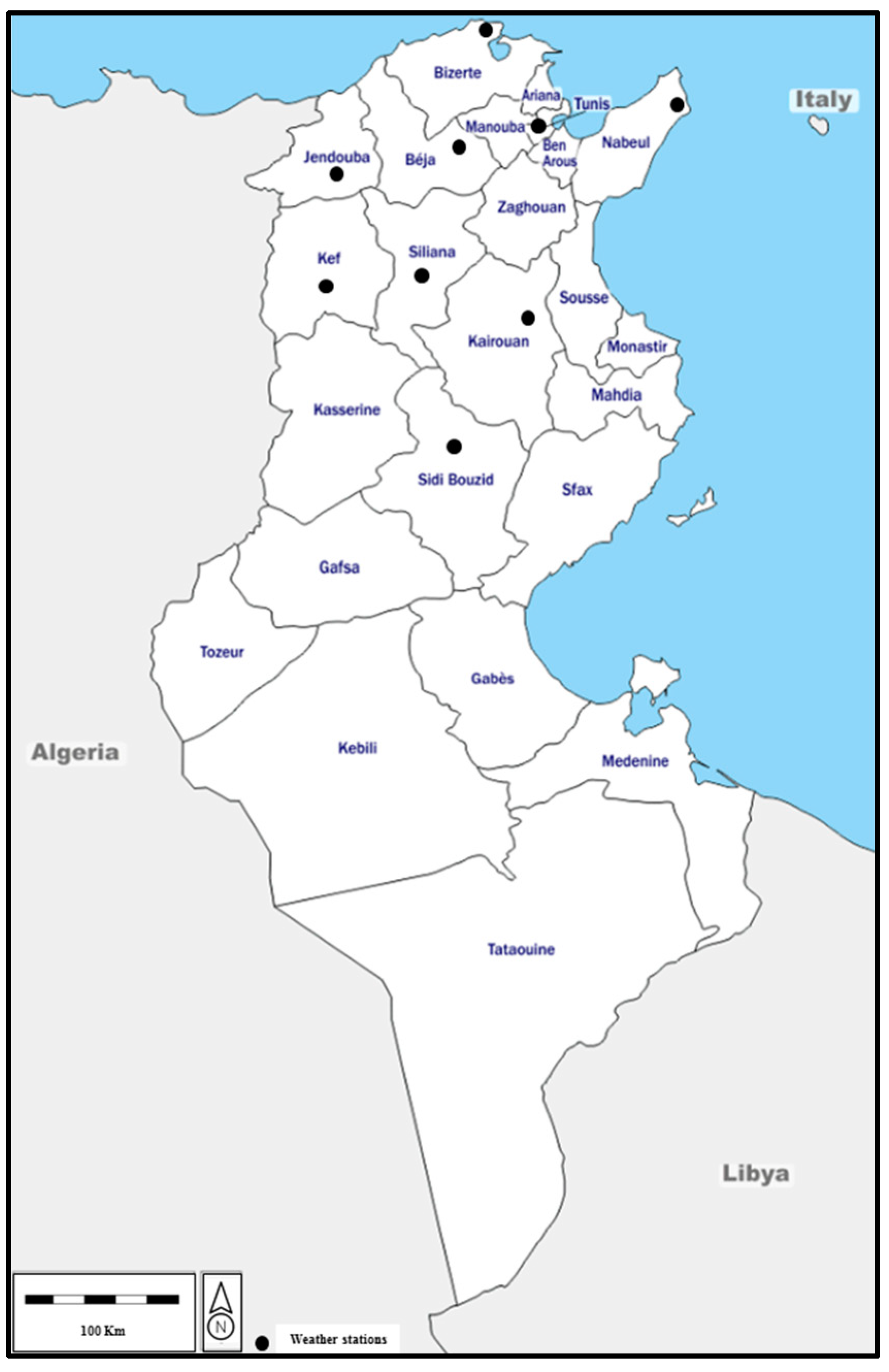
2.1. Research Area

The research has been conducted in nine different locations in the center and north of Tunisia, positioned between 35.00° and 36.85° N in latitude and 8.08° and 11.1° in longitude (Table 1). Among the nine studied locations (Figure 1), three of them are used for training and testing phases, and the remaining are used for estimating ETo in nearby weather stations (production phase), as listed in Table 1. The studied regions are characterized by agricultural activities with irrigated and rainfed crops. The most important irrigated crops in these regions are arable crops (wheat and barley), orchards (citrus fruits, peach, olive, grapevine, etc.), and vegetable crops (tomato, potato, chili, etc.). Livestock farming also exists in the studied regions, which relies on the cultivation of irrigated alfalfa and maize crops for feeding the animals. These agricultural activities require an adequate determination of water requirements, which necessitates a correct estimation of reference evapotranspiration.
The studied regions are characterized by rainfall variability ranging from 248.5 mm in the Sidi Bouzid regions to 617.6 mm in the Bizerte region (Table 1). In these regions, seventy-seven percent (77%) of rainfall falls during the wet season (from October to April), with the highest rainfall typically falling in January (an average of 14% of total average annual rainfall). To describe the climate of the considered regions of this study, we have calculated the Emberger quotient (Q2) [53] as follows:
Q 2 = 2000 × P M 2 m 2
where P is the average annual precipitation (mm), M is the average maximum temperature of the hottest month (°K) (T + 273 °K), and m is the average minimum temperature of the coldest month (°K) (T + 273 °K).
Results showed that most of the studied regions belong to the semi-arid bioclimatic level or zone, with values of Q2 ranging from 34.2 to 60.9, except the regions of Kairouan and Sidi Bouzid, with values of Q2 of 24.1 and 19.5, respectively (Table 1) [53]. The values of Q2 shown by Kairouan and Sidi Bouzid are a little bit close to those characterizing the semi-arid bioclimatic zone.

2.2. Meteorological Data Overview

Monthly climate data from the weather stations is used, including wind speed (WS), solar radiation (SR), relative humidity (RH), maximum temperature (Tmax), and minimum temperature (Tmin). The climatic data used in the study is sourced from the National Institute of Meteorology in Tunisia (NIM), which provides reliable meteorological data. To ensure accuracy, the NIM has installed different kinds of sensors for measuring air temperature (thermometer), relative humidity (hygrometer), wind speed (anemometer), and solar radiation (pyranometer) in a controlled environment covered with grass as a reference crop. These sensors, installed 2.0 m above the ground, continuously register these climatic parameters at an hourly interval, and the collected data are transmitted to a computing system. The Penman–Monteith formula is then applied to calculate the daily ETo values (24 h), providing a robust and scientifically grounded foundation for our study. The 24 h calculation time step has proven to be relatively consistent and accurate for estimating ETo [8,54,55]. The author [54] recommended that no changes are suggested for the FAO-56 PM method for daily (24-h) time steps, where the use of surface resistance of 70 s m−1 should continue. Some weather stations are equipped with a Class A Evaporation Pan, which is a standardized measurement of water loss through evaporation.
We should indicate that these climatic parameters are commonly recognized as important factors influencing evapotranspiration processes. Wind speed plays a crucial role in determining the rate of evaporation by affecting the exchange of moisture between the land surface and the atmosphere. Higher wind speeds generally enhance evaporation rates, as they promote faster moisture transfer and reduce the resistance of the boundary layer. Temperature (minimum and maximum) affects the rate of evapotranspiration through its impact on both evaporation and transpiration. Higher temperatures generally increase the vapor pressure deficit, leading to higher evapotranspiration rates. The mean temperature represents the average temperature over a specific period and provides a measure of the overall thermal conditions. It helps capture the cumulative effect of temperature on evapotranspiration. Solar radiation is a key driver of evapotranspiration, as it provides the energy required for water phase changes. It affects the availability of energy for evaporation and influences the vapor pressure deficit. Relative humidity represents the amount of moisture present in the air relative to its capacity at a given temperature. It influences the vapor pressure deficit and thus affects the potential for evaporation. By including these specific parameters in the ANN model, the study aims to account for the key climatic factors that contribute to evapotranspiration processes. The selection of the input parameters used in the ANN model was also based on data availability and a literature review. The availability of historical climatic data for the study area is essential. The literature review and references provide us with guidance and recommendations about the most important parameters that can be used for reference evapotranspiration modeling.
Table 2 presents the statistical parameters for each variable, such as the mean (Xmean), standard deviation (Sx), coefficient of variation (Cv), skewness coefficient (Csx), minimum (Xmin), and maximum (Xmax). In order to detect the meteorological parameters that most contribute to variations in ETo, we performed a correlation analysis between the FAO-56 PM ETo estimates and each input meteorological parameter (Table 2). The results displayed that the highest correlation coefficients were for Tmax (R = 0.937), followed by SR (R = 0.900) and Tmin (R = 0.817). Wind speed showed a very low value of R, with an average value of 0.030. Relative humidity (RH) displayed a negative coefficient of correlation averaging −0.797, which means that reference evapotranspiration decreases when RH increases. The higher the temperatures rise, the more solar radiation received by the vegetation canopy increases. According to [3], evaporation and transpiration rates increase to satisfy the higher demand for water from the surrounding air. Figure 2 shows the seasonal variation of reference evapotranspiration with respect to elevation.
It seems that there is a significant variation in the values of ETo based on the region’s altitude. The results indicate a positive correlation between altitude and evapotranspiration for the spring and summer seasons, while the correlation is less pronounced in the fall and practically absent in the winter. During the summer, ETo values increase with altitude, indicating a positive relationship. This could be attributed to factors such as a decrease in average temperature and a reduction in potential evaporation at higher altitudes. The high correlation coefficient (0.56) suggests a moderate relationship between altitude and ETo in the summer. During the spring, the positive correlation (R = 0.51) also indicates an increase in ETo with altitude in the spring. However, it is crucial to analyze other potential variables influencing this relationship, such as variations in solar radiation and relative humidity. For the fall season, although the correlation is positive (R = 0.38), it is less pronounced. Seasonal factors that are specific to a given region, such as less precipitation and cooler temperatures, may help to explain this. The very low correlation in winter (R = 0.03) suggests an almost non-existent relationship between altitude and ETo during this season. Seasonal variations specific to winter, such as the presence of snow or reduced sunlight, might influence these results.

2.3. Artificial Neural Network (ANN)

Artificial neural networks (ANNs) are an imitation of the structure and function of biological nervous systems [12,13]. This study used a modular feed-forward neural network (MFFNN), which is a type of ANN and the simplest form of neural network. In an MFFNN neural network, the information flows in one direction from input to output (Figure 3). MFFNN consists of one input layer, one or more hidden layers, and one output layer [56]. The hidden layer is composed of several neurons, also called nodes. The number of PEs was determined empirically by trial and error. The NeuroSolution software (version 5.0) is used in this study [57]. MFFNNs are trained using the Momentum learning algorithm.
A total of 396 monthly climate data points were collected for the regions, and they were divided into three groups. Fifty percent (50%) for training the MFFNN (from January 1974 to June 1990), 25% for cross-validation (from July 1990 to September 1998), and 25% for testing (from October 1998 to December 2006). Figure 4 represents the flowchart of ANN, which is a visual roadmap, delineating the sequential processes from input reception to output generation and providing a clear and systematic representation of the ANN’s functioning.
For training the MFFNN, only the data from three weather stations was used, as listed in Table 1. The three weather stations belong to different locations in Tunisia. Jendouba is in the northwest, Kairouan is in the center, and Kélibia is situated in a coastal region of Tunisia. The underlying idea was to train MFFNN for these three distinct locations. By using these pre-trained models, the goal was to estimate ETo for other regions with the same climatic characteristics without going through the entire training process, which is a time-consuming process. The MFFNN trained for the weather station in Jendouba was used to estimate ETo for the Beja and Le Kef weather stations. During the training process, the option of the use of genetic algorithm (GA) for optimizing the weights of connections between neurons was used. By leveraging the GA, we systematically explored and adjusted the weights, biases, and potentially the architecture of the ANN. This iterative optimization aimed to discover the most effective combination of parameters that would minimize the prediction error and enhance the overall performance of the model. The use of the GA provided a systematic and efficient approach to navigate the complex parameter space, contributing to the improved accuracy and reliability of the optimized model.
The MFFNN trained for the weather station in Kairouan was used to estimate ETo for the Siliana and Sidi Bouzid weather stations. The MFFNN trained for the weather station in Kélibia was used to estimate ETo for Tunis and Bizerte weather stations. This approach allowed for generalizing the estimates to diverse geographical locations without the need to repeat the training process.
To improve the generalization capacity of the ANN, a normalization process was applied to both the input and output data. This normalization was carried out to scale the data values within a specific range, which in this case was set to range from 0 to 1. The normalization process followed this equation:
X n o r m = X i X m i n X m a x X m i n
where Xnorm is the normalized value of the data point; Xi is the original value of the data point; Xmin is the minimum value in the data set; and Xmax is the maximum value in the data set.
To make a correct comparison between the FAO-56 PM and MFF neural network models for ETo estimation, the same data set used to apply the FAO-56 PM equation was also applied to train MFF neural network models. The calculated values of ETo, using the FAO-56 PM equation, were employed as desired data for NeuroSolution software (Version 5.0) execution. The most effective set-up was identified using 1 and 2 hidden layers, from 1 to 30 PE in each hidden layer, and 1000 to 10,000 iterations.

2.4. Modular Feedforward Neural Network Combinations (MFF)

Different combinations of the input parameters were used to train the MFFNN models to estimate daily ETo. A total of eleven (11) combinations are constructed and are listed in Table 3. The first six MFF are one-variable models that each use one parameter independently designed to study the influence of each parameter on the estimation of ETo. The remaining five MFF models each use combinations of two or more meteorological parameters to study how they interact with each other to impact ETo estimation.
  • The MFF-1 model utilizes WS as its main input. This model focuses on analyzing and interpreting WS data, which can be crucial in various applications such as in sprinkler irrigation network design;
  • The MFF-2 model is centered on the input variable of minimum temperature (Tmin). It is specifically designed to analyze the variations in Tmin, making it suitable for studying nighttime weather conditions and frost risks;
  • The MFF-3 model is based on the input variable of maximum temperature (Tmax), and it will also be used to make a comparison with the Turc equation for ETo estimation [8];
  • The MFF-4 model focuses on the input variable of mean temperature (Tmean), and it is used to make a comparison with the FAO 24 Blaney–Criddle model [9];
  • The MFF-5 model is based on the input variable of solar radiation (SR). It is specifically designed to analyze and interpret SR levels, which can be relevant in solar energy applications;
  • The MFF-6 model is centered on the input variable of relative humidity (RH). It is tailored to analyze and interpret relative humidity levels, which can be important in fields such as agriculture, meteorology, or human health;
  • The MFF-7, MFF-8, MFF-9, and MFF-11 models involve combinations of multiple input variables, and they were designed to study the influence or the interaction between climatic parameters;
  • The MFF-10 model has all the parameters that CropWat 8.0 needs to figure out ETo using the FAO-56 PM equation.

2.5. Models’ Performance

The predictive quality of the models was assessed using four statistical criteria: (i) the coefficient of correlation (R), the index of agreement (d), the mean absolute error (MAE), and the root mean square error (RMSE).
The coefficient of correlation (R) is a statistical measure of the strength of the relationship between the observed and forecasted data [58]. Values of R approaching 1.0 indicate strong model performance.
R = i = 1 n X i X ¯ × Y i Y ¯ i = 1 n X i X ¯ 2 × i = 1 n Y i Y ¯ 2
The index of agreement (d) is a statistical measure of the degree of agreement between two continuous variables varying from 0.0 to 1.0 [59]. Index of agreement values close to 1.0 indicate a good fit between measured and predicted ETo.
d = 1 i = 1 n ( Y i X i ) 2 i = 1 n Y i X ¯ + X i X ¯ 2
The root mean square error (RMSE) assesses the disparity among measured and predicted data [60]. Lower values of RMSE mean good model performance.
R M S E = i = 1 n X i Y i 2 n
The mean absolute error (MAE) measures the average absolute discrepancy between measured and predicted values in a dataset. Values of MAE can range from 0 to infinity, and lower values indicate greater predictive accuracy of the model [61].
M A E = 1 n × i = 1 n X i Y i
where Xi is the measured value, Yi is the estimated value, n is the number of observations, X ¯ is the average measured value, and Y ¯ is the average estimated value.

3. Results and Discussion

3.1. Comparison of ETo Conventional Estimation Equations

Table 4 provides the statistical results of the most commonly used ETo estimation models used in Tunisia (the Blaney–Criddle, Riou, and Turc models) during the period of 1974–2006 for the weather stations of Jendouba, Kairouan, and Kélibia. The results have been contrasted with the universal ETo estimation method of Penman and Monteith (EToPM). A quotient between the ETo of the evaluated model (EToModel) and the EToPM model has been calculated to evaluate the degree of estimation.
For the region of Jendouba, it is clear that the three evaluated models underestimated the reference evapotranspiration compared to the PM model (Figure 5). The percentage of underestimation varies widely from one model to another (21.9% for EToBC, 1.9% for EToRIOU, and 66.1% for EToTURC). With performance metrics of 0.850 (R2), 1.130 mm day−1 (MAE), and 1.480 mm day−1 (RMSE), the Riou model exhibited outstanding results.
Figure 6a shows that the underestimation of EToRIOU was concentrated principally during the dry season. On the other hand, it was clear that the Turc model could not estimate the real value of ETo for the region of Jendouba. The performance analysis revealed that the EToTURC model demonstrated comparatively inferior results, with R2, MAE, and RMSE values of 0.90, 3.59 mm day−1, and 4.13 mm day−1, respectively. Figure 6a reveals that the underestimation of EToTURC is distributed throughout the entire period of study (1974–2006) and becomes more pronounced during the dry season.
Regarding the region of Kairouan, the BC and Turc models underestimated the value of ETo compared to the PM model, with percentages of underestimation of 7.1% and 45.6%, respectively (Figure 5). The Riou model overestimated the value of ETo compared to the PM model with a percentage overestimation of 0.9%. Contrary to this, the BC model showcased superior performance statistics, achieving values of 0.87 for R2, 0.85 mm day−1 for MAE, and 1.10 mm day−1 for RMSE. The underestimation of EToBC is evenly distributed throughout the entire study period (1974–2006) (Figure 6b), with an average value of 0.5%. Regarding the Jendouba region, the EToTURC model demonstrated less favorable performance statistics, registering values of 0.89 for R2, 3.14 mm day−1 for MAE, and 3.42 mm day−1 for RMSE. Figure 6b reveals that the underestimation of EToTURC is distributed throughout the entire period of study (1974–2006) and becomes two to three times higher during the dry season.
For the region of Kélibia, the results show that the BC and Riou models overestimated the ETo values compared to the PM model, with percentages of overestimation of 25.0% and 9.1%, respectively (Figure 5). On the other hand, the Turc model continues to underestimate ETo values with a percentage of 24.6%. In terms of performance metrics, the Riou model showcased the most favorable outcomes, recording 0.89 for R2, 0.57 mm day−1 for MAE, and 0.71 mm day−1 for RMSE. The overestimation of the EToRIOU values is more or less evenly distributed throughout the study period (1974–2006), with an average value of 0.4%, and becomes more accentuated during the dry season, as shown in Figure 6c. The same conclusion can be drawn for the Turc model as for the Jendouba and Kélibia regions, with an ETo underestimation of 24.6%.
The evaluation suggests that both EToBC and EToRIOU equations can be used for estimating evapotranspiration in the given regions. EToRIOU generally performs slightly better than EToBC in terms of MAE and RMSE, indicating higher accuracy. However, EToBC tends to have slightly higher R2 values, indicating a better fit with the data. For the three studied regions, the statistical performance of the EToTURC model compared to the PM model does not encourage its use for estimating ETo.
Overall, the choice of ETo calculation method appeared to influence the accuracy of ETo estimation in the evaluated regions. These findings highlight the importance of selecting an appropriate ETo calculation method based on regional characteristics and the desired level of accuracy in estimating evapotranspiration. These region-specific factors in Tunisia can contribute to the observed differences in the performance of the EToBC and EToRIOU formulas across different localities. It is important to consider these regional parameters when choosing the most appropriate method for estimating reference evapotranspiration in each Tunisian region.

3.2. Hiding Layers and Neurons Determination

According to the study by [15], it is possible to determine the nonlinear complex relationship for ETo by using a single hidden layer (HL). In this study, we seek to further investigate the effectiveness of model performance by employing a configuration with two HLs. The selection of the HL’s neurons was accomplished through a process of trial and error. ANNs were trained by varying the number of PEs, ranging from 1 to 20. Following each training iteration, the RMSE, the MAE, and the R2 were computed exclusively using the test dataset. This iterative approach aimed to identify the most suitable number of hidden nodes that resulted in optimal model performance. Two configurations of modular feed-forward neural networks were tested: a first configuration with only one hiding layer (1 HL) and a second configuration with two hiding layers (2 HL).
Figure 7 illustrates how altering the number of PE within the HL impacts the accuracy of the network. In this research, the ideal number of PE within the HL was determined to be nineteen (19) for the “1 HL” configuration. This determination was reached by considering the criteria of minimizing RMSE and MAE while simultaneously maximizing R2. The model attained an R2 value of 0.995, a MAE of 0.183 mm day−1, and a RMSE of 0.323 mm day−1. When using two hiding layers, the best configuration was found to have seven PEs, which gave excellent performance metrics of 0.997 for R2, 0.139 mm day−1 for MAE, and 0.209 mm day−1 for RMSE. Comparing the first configuration, there is a decrease in MAE and RMSE by 24.6% and 35.3%, respectively. On the other hand, there is a small increase in the R2 value of 0.2%. Therefore, the model configuration featuring two hidden layers and seven neurons (2-7-1) was selected as it yielded the most favorable outcomes, and this configuration was subsequently employed to accurately model the ETo. Subsequently, the research conducted a comparison between the estimated ETo obtained through the modular feed-forward neural network (MFF) and the values calculated using the FAO-56 Penman–Monteith (PM) model.
Several research studies have used the FAO-56 PM method to figure out ETo using the ANN technique. They found that the best ANN configuration usually has more than one HL and less than ten PE [13,19,29,38,43,62]. The author [43] used multilayer perceptron ANN (MLP) for estimating ETo as a function of the maximum and minimum temperatures of the air. They found that the best network configuration is 4-6-1 with six PE in the HL and R2 values ranging from 0.81 to 0.84. The author [19] developed a generalized ANN (GANN) corresponding to the FAO-56 PM estimation method. They determined that the optimal GANN architecture is 6-7-1, consisting of seven neurons in each hidden layer, achieving an impressive R2 value of 0.94 when comparing observed and predicted ETo estimates. In a similar vein, the author [29] constructed an ANN for ETo estimation, utilizing eight neurons in each hidden layer and achieving low RMSE values of 0.223 mm day−1.

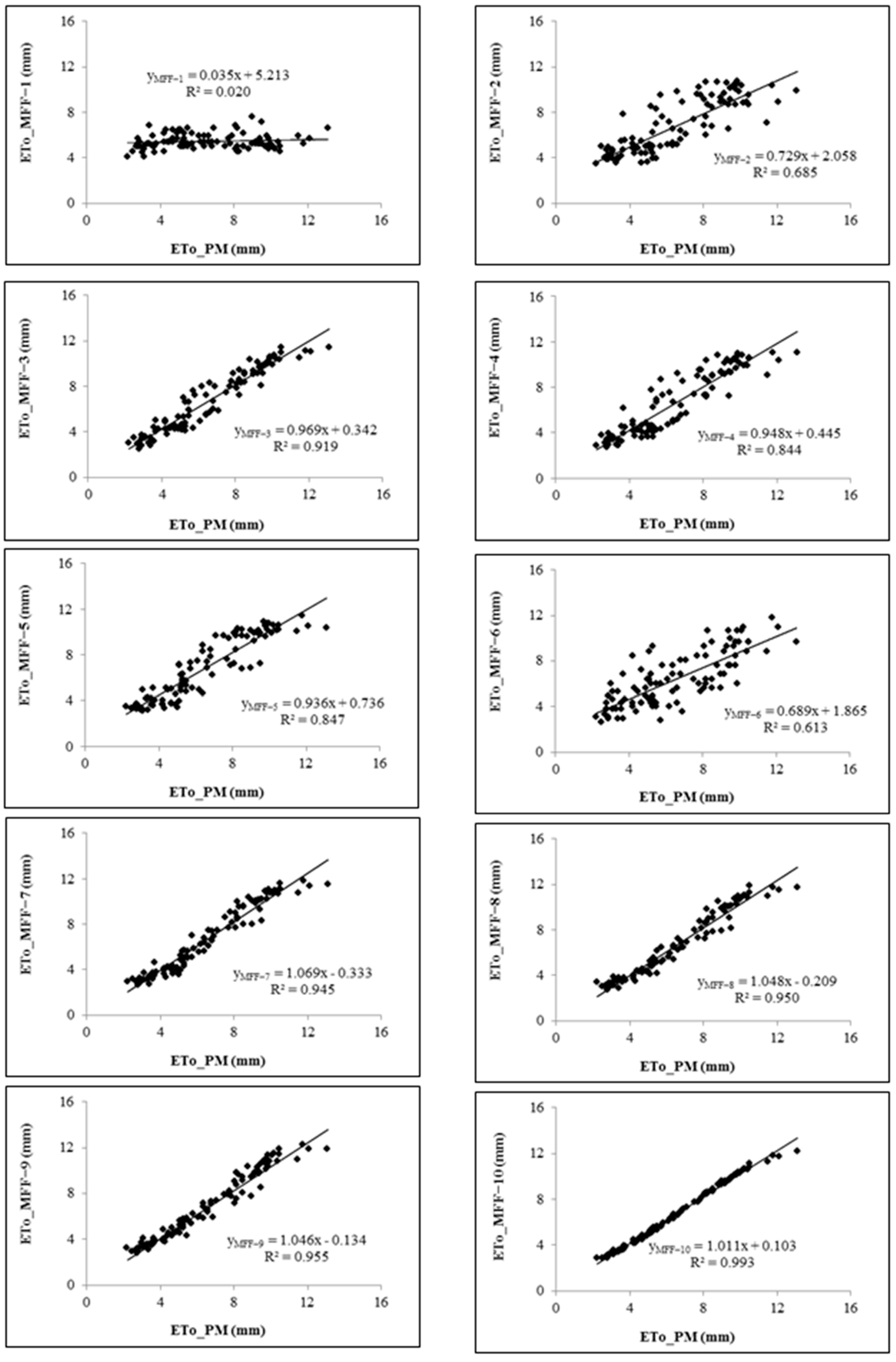
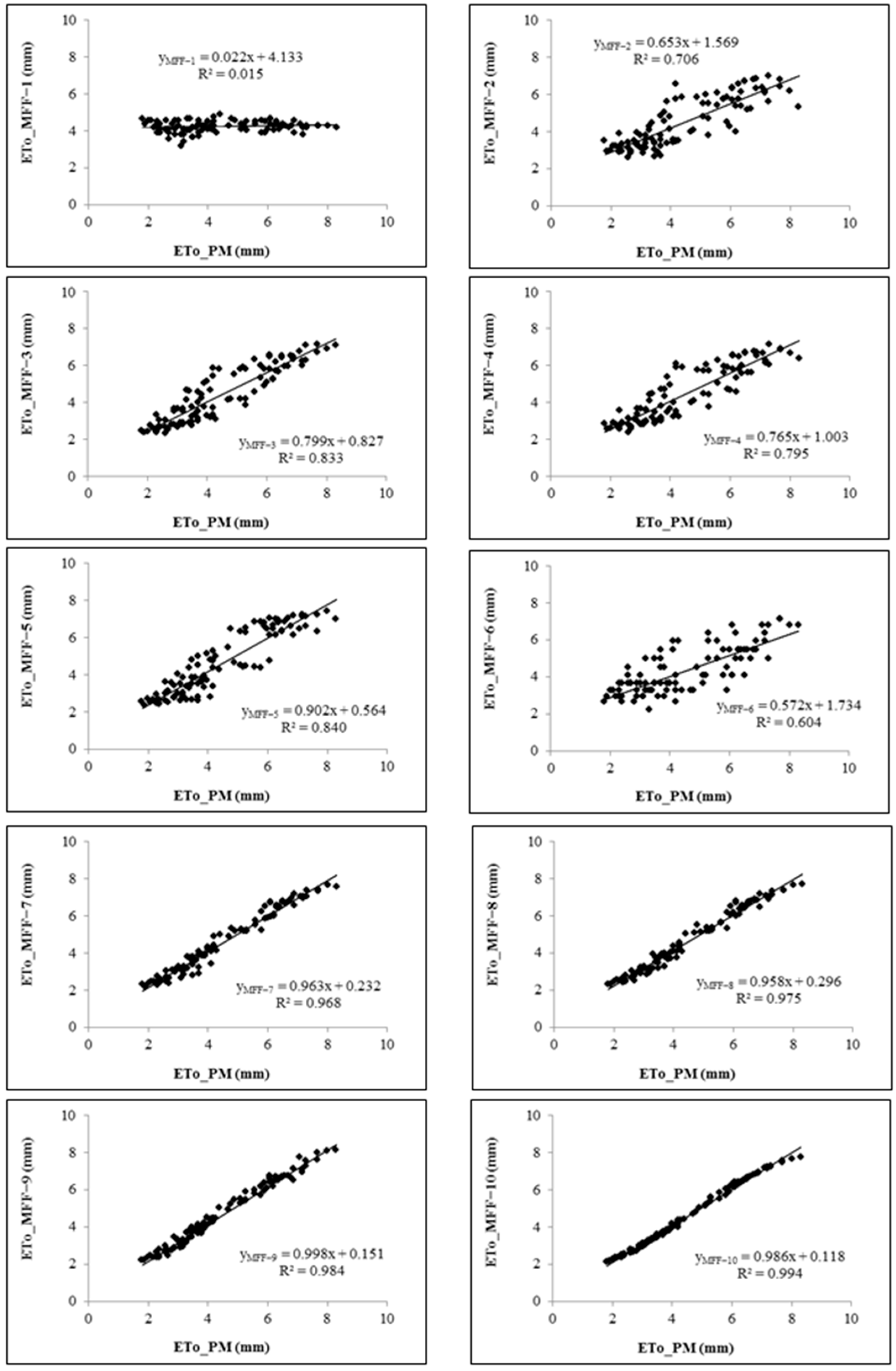
3.3. Most Influential Meteorological Parameters on ETo Modeling

The study uses MFF models with different combinations of six meteorological parameters as inputs (Table 3) to find out how much these parameters affect the estimate of ETo. The first six MFF models each use one parameter independently. The remaining five MFF models each use combinations of two or more parameters.
Table 5 presents the accuracy of the MFF models during the testing period for Jendouba, Kairouan, and Kélibia weather stations. Each model is evaluated based on its R2, d, MAE, and RMSE values. Figure 8, Figure 9 and Figure 10 show a comparison of ETo estimates predicted using the MFF (ETo_MFF) and FAO-56 PM (ETo_PM) methods for the weather stations in Jendouba, Kairouan, and Kélibia, respectively.
For the three studied regions and within the individual MFF evaluated models (from MFF-1 to MFF-6), the maximum temperature (Tmax), evaluated by the MFF-3, was the most influential meteorological parameter on ETo estimation (Table 5). The MFF-3 statistical performance results ranged from 0.883 to 0.936, 0.950 to 0.983, 0.597 to 0.704 mm day−1, and 0.703 to 0.894 mm day−1 for, respectively, R2, d, MAE, and RMSE. Among the six meteorological parameters considered in this case study, Tmax is the most accurate predictor of ETo. However, adding solar radiation to the MFF-7 input combination made the model work much better, with R2 and d average values going up by 7.1% and 1.8%, respectively. A decrease in MAE and RMSE average values was also noted (29.2% and 27.4%, respectively). The author [11] also found that Tmax was the most influential parameter for accurate estimation of ETo at three weather stations (Santa Monica, Claremont, and Pomona).
On the other hand, according to the MFF-1’s evaluation, wind speed (WS) had the least impact on ETo estimation (Table 5). Actuating individually, WS caused the highest values of MAE and RMSE, ranging from 1.410 to 2.869 mm day−1 and 1.709 to 3.407 mm day−1, respectively. The values of R2 and d were the lowest and ranged from 0.015 to 0.069 and 0.253 to 0.449, respectively. The addition of WS to the input combination of the MFF-10 model improves its accuracy compared to the MFF-9 model, as evidenced by the 2.6% and 0.7% increases in R2 and d values, respectively. Whereas, the values of MAE and RMSE diminished significantly by 53.7% and 56.3%, respectively. This may be due to the advection effect of wind speed on ETo [11]. The author [28] used the generalized regression neural networks (GRNNs) technique to model ETo, obtained using the FAO-56 PM equation, to study the effect of SR, T, RH, and WS on ETo. The author found that using wind speed as a unique input to ANN is insufficient for modeling ETo.
It was quite clear that the Tmin and RH meteorological parameters do not have any effectiveness in improving the predictive quality of MFF-8 with respect to MFF-7 (insertion of Tmin into MFF-7) and of MFF-9 with respect to MFF-8 (insertion of RH into MFF-8). Hence, the average values of R2 and d registered the lowest increments, with values of 0.5% and 0.2%, respectively. It was also found by the author [63] that adding relative humidity as an input to ANNs for estimating ETo in the Bobo Dioulasso region of Burkina Faso does not make the models more accurate. These authors used the FAO-56 PM equation as an estimation method to feed ANNs. They obtained very low RMSE and MAE values of 0.048 mm day−1 and 0.033 mm day−1, respectively.
The mean temperature meteorological parameters (Tmean) influence the estimation of ETo differently from one region to another. The MFF-4’s evaluation of the mean temperature (Tmean), which reached values of R2 and d of 0.868 and 0.964, respectively, estimated ETo for the Jendouba region better than the other remaining meteorological parameters, with the exception of Tmax. For the regions of Kairouan and Kélibia, it seems that solar radiation (SR), evaluated by the MFF-5, performed better than Tmean in the estimation of ETo, despite the fact that the statistics were very close with minimal differences. Several studies found that solar radiation significantly enhanced the predictive quality of ANN for ETo modeling [12,64,65]. These authors used climatic parameters on daily and monthly time steps as inputs to ANN models to predict ETo given by the FAO-56 PM method.
MFF-10 was found to be the most accurate model in terms of MAE and RMSE (0.183 mm day−1 and 0.241 mm day−1, respectively) and the highest R2 and d (0.993 and 0.998, respectively) average statistics. This model integrates almost all the meteorological parameters as inputs (Tmax, Tmin, WS, SR, and RH). This result indicates that the more climate variables are incorporated into the neural networks, the more the predictive quality of the models significantly improves. This suggests that the inclusion of the Tmax, Tmin, SR, RH, and WS parameters is indispensable for enhancing the modeling of reference evapotranspiration. The author [11] also found that the estimation of ETo using ANN is more accurate when all of the meteorological parameters considered for the three tested weather stations were used as inputs. The author [66] used ANN to forecast ETo from daily climatic parameters (Tmax, Tmin, WS, SR, and RH) for sustainable irrigation scheduling. In this case study, the FAO-56 PM equation was used as the reference method for comparison purposes. The authors concluded that the robustness and accuracy of the forecasted models may help farmers, water resource managers, and irrigation planners with improved and sustainable water management at the basin level and irrigation scheduling at the farm or field level.
Average monthly estimated ETo values obtained by the MFF-10 model for Jendouba, Kélibia, and Kairouan weather stations were compared with average monthly observed values of ETo. Figure 11 compares average monthly ETo estimates predicted by the MFF-10 model with average monthly observed values for the respective weather stations in Jendouba, Kairouan, and Kélibia. The observed ETo values were measured directly using the PAN method. The correlation results between the estimated monthly mean values of ETo by the MFF-10 model and the observed monthly mean values of ETo for the three regions were 0.935, 0.935, and 0.912 for, respectively, Jendouba, Kélibia, and Kairouan (Figure 11). These correlation coefficients indicate a strong positive relationship between the ETo estimates provided by the MFF-10 model and the observed ETo values for each respective region. The high correlation values near 1.0 suggest that the model’s estimations closely align with the observed data, reinforcing the reliability and accuracy of the MFF-10 model in predicting annual mean ETo values for the Jendouba, Kélibia, and Kairouan regions.
Based on these results, it is clear that Tmax is the most significant weather factor for accurately simulating the complicated and nonlinear process of evapotranspiration in the Jendouba, Kairouan, and Kélibia regions. The integration of SR and WS parameters improves the accuracy of the models and could be classified as sensitive meteorological parameters in the estimation of ETo. The SR and WS inputs were also found to be the most influential climatic parameters in the modeling of ETo [67]. The author [68] observed that for accurate estimation of ETo using an ANN, temperature and radiation data are the most crucial inputs. Another case study revealed that wind speed contributes more significantly to errors in ETo than solar radiation [69]. The authors [11] found that RH and WS had the greatest influence on ETo estimation, which is different from our results. All these authors used the FAO-56 PM equation to generate ETo observed measurements from climatic data in order to use it as the desired target to train and test constructed ANN models.

3.4. Comparison ETo Estimation Models and ANNs Models

This section compares the FAO-56 PM, the FAO-24 BC, the Riou, and the Turc empirical equations with the corresponding MFF-10, MFF-4, MFF-11, and MFF-3, respectively. Table 6 presents a comparison between MFF neural network models and the corresponding ETo estimation model.

3.4.1. Jendouba Weather Station

The FAO-24 BC method appears to have a slightly higher R2 value of 0.884, indicating a slightly better fit to the data compared to MFF-4 (R2 = 0.864). However, MFF-4 has a lower MAE and RMSE of 1.005 mm day−1 and 1.252 mm day−1, respectively. This result suggests that MFF-4 may provide more accurate estimates overall, despite a slightly lower R2 value. MFF-11 clearly outperforms the Turc method in terms of R2, MAE, and RMSE, reaching values of 0.961, 0.572 mm day−1, and 0.779 mm day−1, respectively. This result implies that MFF-11 provides better estimates of evapotranspiration in this context. The MFF-3 model does much better than the Riou method. It has higher R2, MAE, and RMSE values of 0.936, 0.704 mm day−1, and 0.894 mm day−1, respectively. This means that the MFF-3 model gives more accurate estimates of ETo than the Riou equation in this case.
In summary, based on these findings, MFF-4 appears to perform slightly better than FAO-24 BC, MFF-11 outperforms the Turc method, and MFF-3 demonstrates high accuracy compared to the Riou method in the estimation of ETo. The choice between these methods may depend on specific application requirements and data availability.

3.4.2. Kairouan Weather Station

MFF-4 outperforms the FAO-24 BC method in terms of R2 and RMSE (0.919 and 0.784 mm day−1, respectively). It can be deduced from these findings that MFF-4 provides better estimates of evapotranspiration in this context. Both methods have similar MAE values. MFF-11 significantly outperforms the Turc method in terms of R2, MAE, and RMSE, with an increment value of 3.6% for R2 with respect to the Turc equation and a high decrease in MAE and RMSE values of 78.8% and 75.6%, respectively, compared to the Turc model. These results point to the fact that MFF-11 provides more accurate estimates of evapotranspiration compared to Turc in this particular scenario. MFF-3 outperforms the Riou method in terms of R2 and RMSE, with values of 0.919 and 0.784 mm day−1, respectively. It appears from these findings that MFF-3 provides more accurate estimates of evapotranspiration compared to Riou in this particular scenario. Both methods have similar MAE values.
In summary, based on the results of the Kairouan weather station, MFF-4 appears to perform better than FAO-24 BC, MFF-11 outperforms the Turc method, and MFF-3 is more accurate than the Riou method in estimating evapotranspiration. The choice between these methods may depend on specific application requirements and data availability.

3.4.3. Kélibia Weather Station

The FAO-24 BC method appears to have a moderately higher R2 value, indicating a slightly better fit to the data compared to MFF-4 (0.911 and 0.795, respectively). However, MFF-4 has a lower MAE and RMSE, with an average of 45% difference compared to the FAO-24 BC method. These findings pinpointed that MFF-4 may provide more accurate estimates overall, despite a moderately lower R2 value. MFF-11 significantly outperforms the Turc method in terms of R2, MAE, and RMSE, indicating that MFF-11 provides more accurate estimates of evapotranspiration compared to Turc in this particular scenario. Riou outperforms MFF-3 in terms of R2 and RMSE, indicating that Riou provides slightly better estimates of evapotranspiration compared to MFF-3 in this specific context. However, both methods have similar MAE values.
In summary, based on the provided data, FAO-24 BC performs better than MFF-4 in terms of R2 values. In terms of MAE and RMSE statistics, MFF-4 performs better in the estimates of ETo compared to the FAO-24 BC model. MFF-11 outperforms the Turc method, and Riou has a slight edge over MFF-3 in estimating evapotranspiration. The choice between these methods should consider specific application requirements and data availability.
Generally, for the Jendouba region, MFF-3 and MFF-4 seem to be the preferred methods for estimating ETo, as they outperform conventional methods like FAO-24 BC and Turc. In the case of the Kairouan region, MFF-4 and MFF-11 offer better ETo estimates compared to FAO-24 BC and Turc. And finally, for the Kélibia region, FAO-24 BC performs well, and MFF-11 outperforms Turc, while Riou is competitive with MFF-3. In general, the choice of the most suitable method for estimating ETo should consider the specific region’s climate characteristics and data availability. MFF-4 and MFF-11 often provide accurate estimates across multiple regions, but the performance of conventional methods like FAO-24 BC and Turc may also vary depending on the location. It is essential to select the method that best suits the local conditions and data quality.
Similar conclusions were also obtained by several researchers when comparing the performance of ANN in estimating ETo with respect to conventional methods. For example, the authors [33,34] found that the radial basis function neural network model performed better estimates of ETo than the Turc and Blaney–Criddle models in different agro-climatic zones. Corresponding results were also achieved by [14] when comparing the predictive accuracy of backpropagation neural network methodology in evapotranspiration forecasting in the Dédougou region (western Burkina Faso) with the conventional method of Blaney–Criddle. The authors [35] investigated the ability of the M5 model tree (M5T), adaptive neuro-fuzzy inference system (ANFIS), and support vector machines (SVM) for modeling daily reference evapotranspiration for the De Soto County station located in Florida. They arrived at the robust conclusion that using computational models such as ANN for ETo estimation yielded better results than conventional methods such as empirical equations.

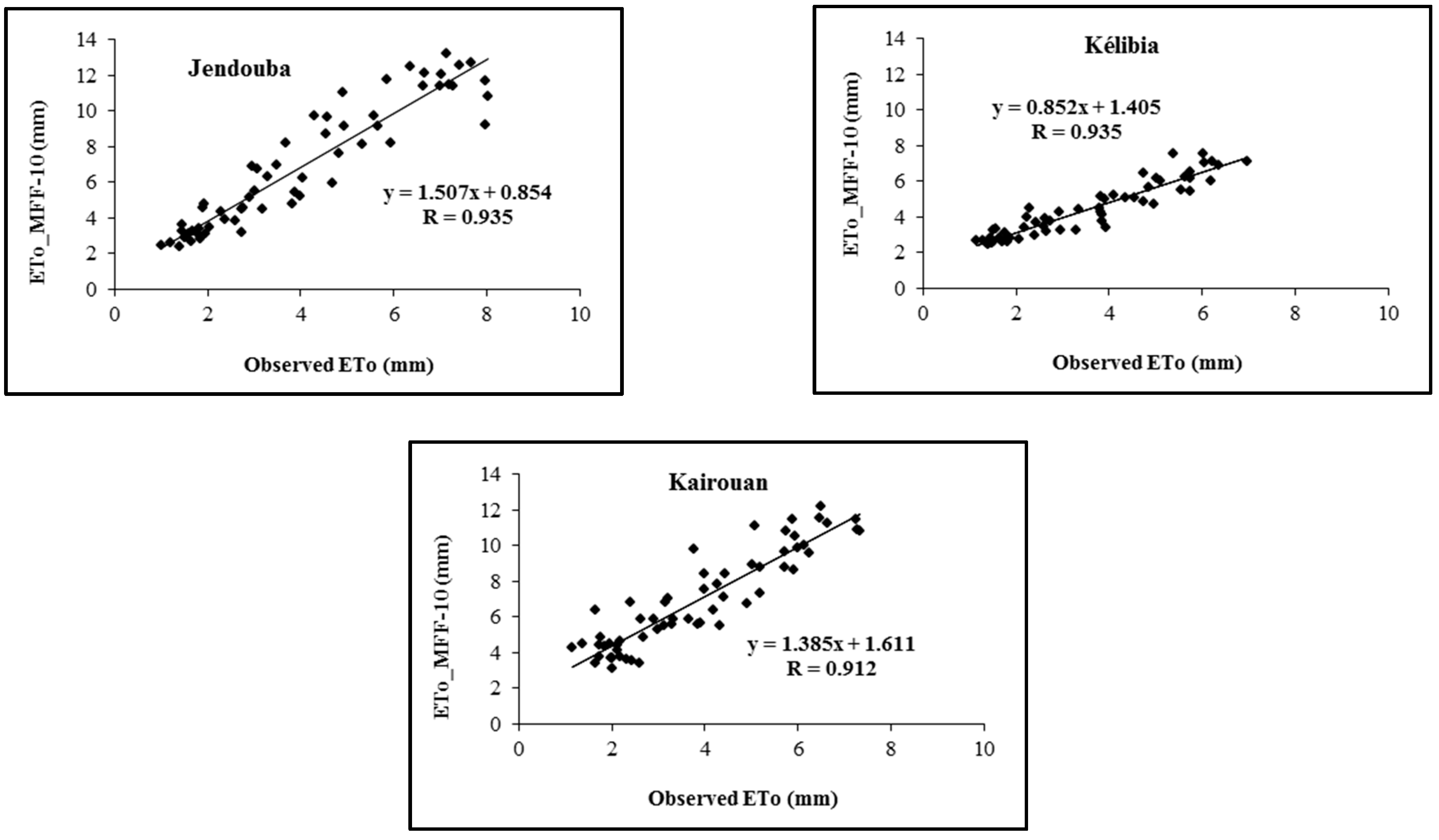
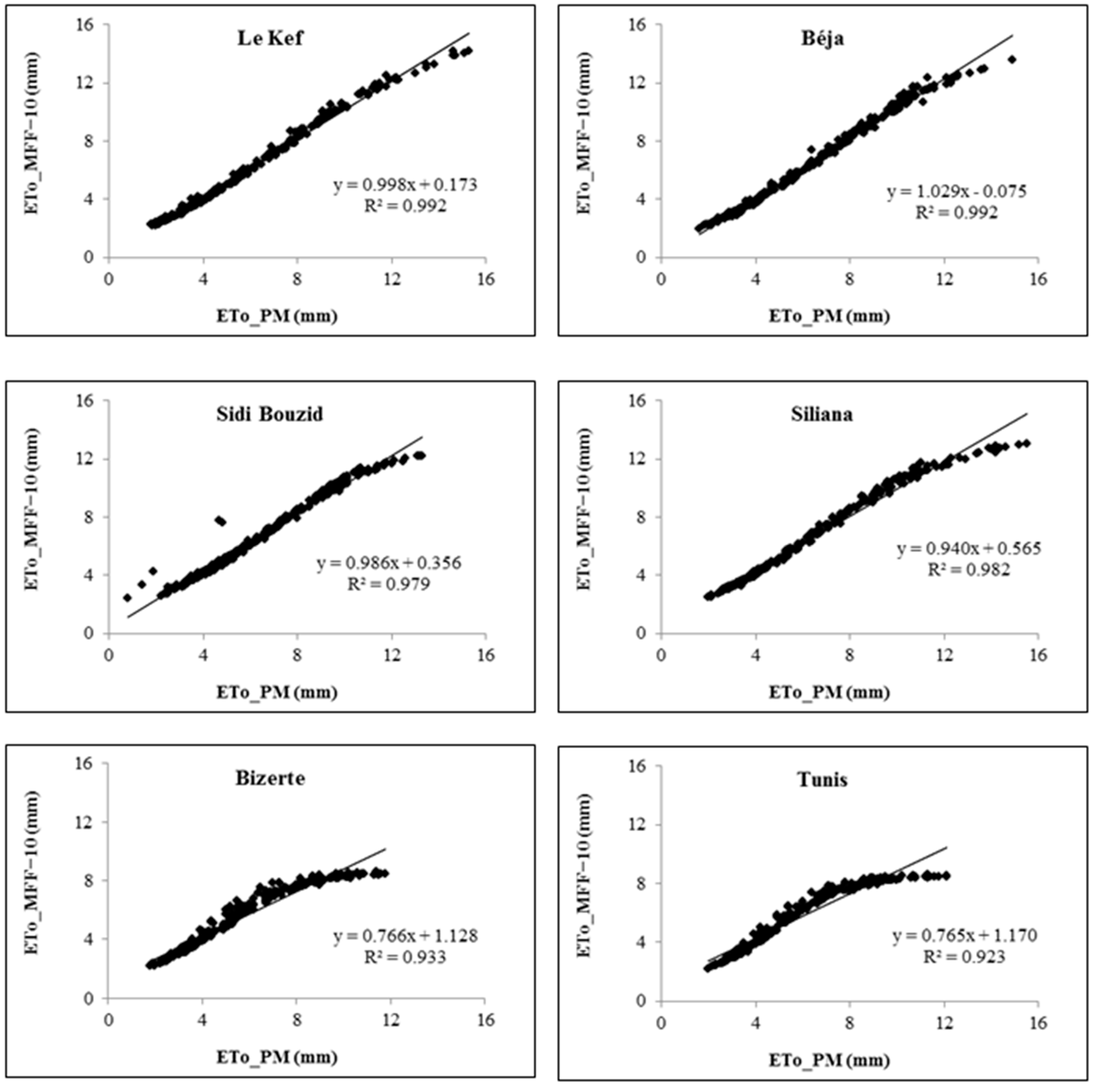
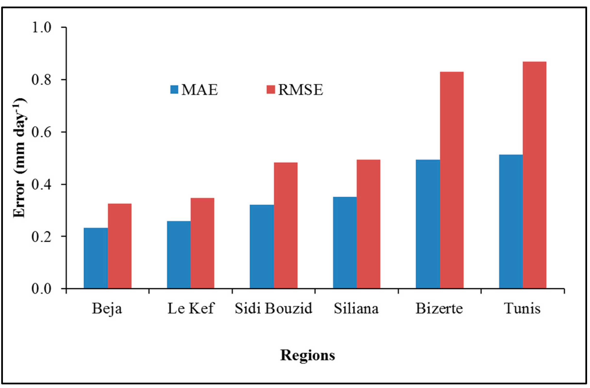
3.5. Reference Evapotranspiration Estimation of Nearby Weather Stations

To assess the transferability of trained artificial neural networks (ANNs) from one weather station to nearby stations, we evaluated the performance of MFF-10 models trained for the three previous weather stations: Jendouba, Kairouan, and Kélibia. These models were employed to estimate reference evapotranspiration at six other weather stations, each one of them using distinct input variables. Specifically, the MFF-10 model trained for Jendouba was utilized to estimate ETo at the Béja and Kef weather stations. Simultaneously, the MFF-10 model trained for Kairouan was applied to estimate ETo at the Siliana and Sidi Bouzid weather stations. Lastly, the MFF-10 model constructed for Kélibia was employed to estimate ETo at the Tunis and Bizerte weather stations. The estimation performance is presented in Table 7, and the statistics were calculated with respect to the FAO-56 PM equation.
The results indicate that reference evapotranspiration can be estimated with high accuracy using trained ANNs for other weather stations with different input variables. Figure 12 shows the scatter plots of ETo as estimated by MFF-10 and FAO 56 PM at Béja and Kef (MFF-10 trained at Jendouba station), Sidi Bouzid and Siliana (MFF-10 trained at Kairouan station), and Bizerte and Tunis (MFF-10 trained at Kélibia station). Figure 13 shows a visual comparison of the MAE and RMSE evaluation metric for the different regions. In general, it should be noted that all the tested regions presented high statistical performance, with values of R2 and d ranging from 0.923 to 0.992 and from 0.964 to 0.997, respectively. On the other hand, MAE and RMSE statistics presented very low values ranging from 0.233 mm day−1 and 0.514 mm day−1 and from 0.326 mm day−1 to 0.869 mm day−1, respectively (Figure 13). These results indicated that ANNs could be a powerful tool to estimate ETo values for nearby stations without the need for training and testing procedures. The close-to-perfect R2 and d values suggest that the MFF-10 model accurately captures the variability of ETo in all regions, making it a highly reliable tool for ETo estimation for nearby weather stations. These findings underscore that the MFF-10 model holds promise as a reliable instrument for ETo estimation, offering valuable insights for irrigation management and water resource planning.
Several research studies tested their trained ANN for stations that were not included during the training process [11,19,29,40,41,62,70,71,72]. The majority of these authors used the standard FAO-56 PM method to calculate ETo values used as targets to train and test ANN models [3]. All the researchers found that ANN with high ETo predictive quality could be applied to yield ETo estimates from other data sets that were not included in the training process. For example, the author [19] developed ANNs trained with respect to the FAO-24 BC ETo estimation method. The findings revealed that the trained ANN models could be applied to produce ETo estimates without any additional input data. The author [71] constructed an ANN using data from three stations and then tested it on five stations that were not included during the training process. He also found that there is no need for additional calibration to estimate ETo in new locations. The author [41] concluded that ANNs can be used with relatively good accuracy for water resource management, irrigation scheduling and management, and environmental assessment when data are not enough to use trained ANNs from another location. The author [40] pinpointed that ANNs with good predictive quality could be generalized to estimate ETo values for areas with similar climatic characteristics.
Our findings represent a significant advancement in our understanding of reference evapotranspiration dynamics in semi-arid bioclimatic regions. By harnessing the power of ANNs, this study not only refines our ability to forecast reference evapotranspiration accurately but also contributes valuable insights into the intricate relationships governing climatic and environmental variables in these regions. The knowledge generated through this research extends beyond its immediate focus, offering a blueprint for similar studies in semi-arid zones globally. The applications of our findings hold promise for enhancing water resource management, optimizing agricultural practices, and bolstering climate change adaptation measures in diverse semi-arid contexts. As such, this research serves as a pivotal resource, bridging gaps in our current understanding and laying the groundwork for practical, data-driven solutions with relevance on a broader, international scale.
This research offers valuable insights and practical tools that can be applied to improve water management and agricultural planning not only in the studied regions but also in other semi-arid bioclimatic regions across the country. The transferability of our methodology and findings provides a foundation for sustainable practices in the face of evolving environmental conditions. The results can be used to improve water resource management through the accurate estimation of reference evapotranspiration. The accurate estimation of ETo is essential for optimizing irrigation practices and determining crop water requirements. This has implications for crop yield optimization and resource sustainability. Our research contributes to the development of robust models that can be instrumental in adapting water management and agricultural practices to changing climate conditions in regions facing similar challenges.

4. Conclusions

Adequate estimation of ETo is a key factor in the correct calculation of irrigation water needs at the field and district scales. In this paper, the climatic data of nine weather stations was used to estimate ETo using the approach of ANN. Among these weather stations, three of them were used to train and test MFFNN, and the remaining were used to estimate ETo using pre-trained MFFNN without going through the entire training process. The following conclusions can be drawn:
  • Both the EToBC and EToRIOU equations attest to being suitable for estimating ETo in the studied regions when compared to the FAO-56 PM model. Conversely, the EToTURC model consistently underestimated ETo values;
  • It has been demonstrated that ANNs are an effective technique for modeling reference evapotranspiration;
  • It was found that Tmax is the most influential meteorological parameter in ETo modeling;
  • However, using only WS as an ANN input was determined to be insufficient for ETo modeling;
  • Nevertheless, inserting WS in the input combinations leads to improved estimation accuracy, primarily because of its influence on ETo through advection effects;
  • On the other side, the use of SR and Tmean gives much better ETo estimates than those obtained using RH and Tmin;
  • The ANN model integrating Tmax, SR, Tmin, RH, and WS performs the best among the input combinations tested in this study, which means that all meteorological parameters are quite important for ETo modeling;
  • It is evident that the use of ANN for estimating ETo consistently provides more accurate estimates of ETo compared to the conventional formulas of FAO-24 BC, Riou, and Turc;
  • It was found that the trained MFF-10 model, which takes into account all meteorological factors, could accurately estimate the ETo for nearby areas when different input variables were used.
In summary, the ANN technique could be used to enhance water management practices at field and district scales. This technique can be used to provide real-time or forecasted information on irrigation scheduling, optimizing water usage, and improving overall efficiency in agricultural irrigation systems. The study relied on data collected from only three stations, suggesting that additional research utilizing a broader dataset from diverse regions may be necessary to strengthen the findings derived from this study. The outcomes of this research offer valuable insights and contributions to the existing literature on ETo estimation. The comparative analysis between ETo estimation formulas utilizing limited input data and the universal FAO-56 PM equation offers a comprehensive insight into their respective effectiveness in estimating evapotranspiration. Secondly, the comparison between the FAO-56 PM method and the ANN technique contributes to the ongoing discourse on the applicability of advanced computational methods for ETo estimation. The identification of the most influential meteorological parameter on ETo estimation contributes to the understanding of the key factors driving evapotranspiration processes. Lastly, the assessment of the accuracy of the ANN technique in estimating ETo using data from nearby weather stations, offers practical insights into the potential advancements and reliability of utilizing ANN in refining ETo predictions, thereby advancing the broader literature on water resource management and agricultural practices.

Author Contributions

Conceptualization, methodology, investigation, writing—original draft preparation, A.S. and A.F.; Methodology, software, data interpretation, data analysis, writing—review and editing, A.B., S.K. and M.A.M.; Software, data analysis, writing—review and editing, A.S. and M.A.M. All authors have read and agreed to the published version of the manuscript.

Funding

The authors extend their appreciation to the Deputyship for Research & Innovation, Ministry of Education in Saudi Arabia for funding this research (IFKSURC-1-4108).

Data Availability Statement

Data are contained within the article.

Acknowledgments

The authors extend their appreciation to the Deputyship for Research & Innovation, Ministry of Education in Saudi Arabia for funding this research. (IFKSURC-1-4108).

Conflicts of Interest

The authors declare no conflicts of interest.

References

  1. Naoum, S.; Tsanis, I.K. Hydro informatics in evapotranspiration estimation. Environ. Model. Softw. 2003, 18, 261–271. [Google Scholar] [CrossRef]
  2. Allen, R.G.; Jensen, M.E.; Wright, J.L.; Burman, R.D. Operational estimates of reference evapotranspiration. J. Agron. 1989, 81, 650–662. [Google Scholar] [CrossRef]
  3. Allen, R.G.; Pereira, L.S.; Raes, D.; Smith, M. Crop evapotranspiration guidelines for computing crop water requirements. In FAO Irrigation and Drainage Paper No. 56; Food and Agriculture Organization of the United Nations: Rome, Italy, 1998. [Google Scholar]
  4. Smith, M.; Allen, R.; Pereira, L. Revised FAO Methodology for Crop Water requirements. In Land and Water Development Division; FAO: Rome, Italy, 1997. [Google Scholar]
  5. Srivastava, A.; Sahoo, B.; Raghuwanshi, N.S.; Singh, R. Evaluation of Variable-Infiltration Capacity Model and MODIS-Terra Satellite-Derived Grid-Scale Evapotranspiration Estimates in a River Basin with Tropical Monsoon-Type Climatology. J. Irrig. Drain. Eng. 2017, 146, 1–18. [Google Scholar] [CrossRef]
  6. Chow, V.T.; Maidment, D.R.; Mays, L.W. (Eds.) Applied Hydrology; McGraw-Hill: New York, NY, USA, 1988. [Google Scholar]
  7. Riou, C. Compte rendu des Journées d’étude de l’Office de la Recherche Scientifique et Technique Outre-Mer; ORSTOM: Paris, France, 1980; p. 373. ISBN 2-7099-0657-0. [Google Scholar]
  8. Turc, L. Evaluation des besoins en eau d’irrigation, évapotranspiration potentielle. Ann. Agron. 1961, 12, 13–49. [Google Scholar]
  9. Doorenbos, J.; Pruitt, W.O. Guidelines for Predicting Crop Water Requirements; FAO: Rome, Italy, 1977; 24p. [Google Scholar]
  10. Elbeltagi, A.; Kumari, N.; Dharpure, J.K.; Mokhtar, A.; Alsafadi, K.; Kumar, M.; Mehdinejadiani, B.; Etedali, H.R.; Brouziyne, Y.; Towfiqul Islam, A.R.M.; et al. Prediction of combined terrestrial evapotranspiration index (CTEI) over large River basin based on machine learning approaches. Water 2021, 13, 547. [Google Scholar] [CrossRef]
  11. Kisi, O.; Ozturk, O. Adaptive neurofuzzy computing technique for evapotranspiration estimation. J. Irrig. Drain. Eng. 2007, 133, 368–379. [Google Scholar] [CrossRef]
  12. Kisi, O. Daily pan evaporation modelling using a neuro-fuzzy computing technique. J. Hydrol. 2006, 329, 636–646. [Google Scholar] [CrossRef]
  13. Landeras, G.; Ortiz-Barredo, A.; López, J.J. Comparison of artificial neural network models and empirical and semi-empirical equations for daily reference evapotranspiration estimation in the Basque Country (Northern Spain). Agric. Water Manag. 2008, 95, 553–565. [Google Scholar] [CrossRef]
  14. Sudheer, K.P.; Gosain, A.K.; Ramasastri, K.S. Estimating actual evapotranspiration from limited climatic data using neural computing technique. J. Irrig. Drain. Eng. 2003, 129, 214–218. [Google Scholar] [CrossRef]
  15. Kumar, M.; Raghuwanshi, N.S.; Singh, R.; Wallender, W.W.; Pruitt, W.O. Estimating evapotranspiration using artificial neural network. J. Irrig. Drain. Eng. 2002, 128, 224–233. [Google Scholar] [CrossRef]
  16. Trajkovic, S.; Todorovic, B.; Stankovic, M. Forecasting reference evapotranspiration by artificial neural networks. ASCE J. Irrig. Drain. Engng. 2003, 129, 454–457. [Google Scholar] [CrossRef]
  17. Keskin, M.E.; Terzi, O. Artificial Neural Network Models of Daily Pan Evaporation. J. Hydrol. Eng. 2006, 11, 65–70. [Google Scholar] [CrossRef]
  18. Gonzalez-Camacho, J.M.; Cervantes-Osornio, R.; Ojeda-Bustamante, W.; Lopez-Cruz, I. Forecasting reference evapotranspiration using artificial neural networks. Ing. Hidráulica México 2008, 23, 127–138. [Google Scholar]
  19. Kumar, M.; Raghuwanshi, N.S.; Singh, R. Development and validation of GANN model for evapotranspiration estimation. J. Hydrol Eng. ASCE 2009, 44, 131–140. [Google Scholar] [CrossRef]
  20. Falamarzi, Y.; Palizdan, N.; Huang, Y.F.; Lee, T.S. Estimating evapotranspiration from temperature and wind speed data using artificial and wavelet neural networks (WNNs). Agric. Water Manag. 2014, 140, 26–36. [Google Scholar] [CrossRef]
  21. Traore, S.; Wang, Y.M.; Chung, W. Predictive accuracy of backpropagation neural network methodology in evapotranspiration forecasting in Dédougou region, western Burkina Faso. J. Earth Syst. Sci. 2014, 123, 307–318. [Google Scholar] [CrossRef]
  22. Raju, K.S.; Kumar, D.N.; Duckstein, L. Artificial neural networks and multi criterion analysis for sustainable irrigation planning. Comput. Oper. Res. 2006, 33, 1138–1153. [Google Scholar] [CrossRef]
  23. Pulido-Calvo, I.; Gutierrez-Estrada, J.C. Improved irrigation water demand forecasting using a soft-computing hybrid model. Biosyst. Eng. 2009, 102, 202–218. [Google Scholar] [CrossRef]
  24. Tsang, S.W.; Jim, C.Y. Applying artificial intelligence modeling to optimize green roof irrigation. Energy Build. 2016, 127, 360–369. [Google Scholar] [CrossRef]
  25. Yang, C.C.; Prasher, S.O.; Lacroix, R.; Sreekanth, S.; Patni, N.K.; Masse, L. Artificial neural network model for subsurface-drained farmlands. J. Irrig. Drain. Eng. 1997, 123, 285–292. [Google Scholar] [CrossRef]
  26. Deka, P.C.; Chandramouli, V. Fuzzy neural network modeling of reservoir operation. J. Water Resour. Plan. Manag. 2009, 135, 5–12. [Google Scholar] [CrossRef]
  27. Thornton, P.E.; Hasenauer, H.; White, M.A. Simultaneous estimation of daily solar radiation and humidity from observed temperature and precipitation: An application over complex terrain in Austria. Agric. For. Meteorol. 2000, 104, 255–271. [Google Scholar] [CrossRef]
  28. Kisi, O. Generalized regression neural networks for evapotranspiration modeling. J. Hydrol. Sci. 2006, 51, 1092–1105. [Google Scholar] [CrossRef]
  29. Dai, X.; Shi, H.; Li, Y.; Ouyang, Z.; Huo, Z. Artificial neural network models for estimating regional reference evapotranspiration based on climate factors. Hydrol. Process. 2009, 23, 442–450. [Google Scholar] [CrossRef]
  30. Ayaz, A.; Rajesh, M.; Singh, S.K.; Rehana, S. Estimation of reference evapotranspiration using machine learning models with limited data. AIMS Geosci. 2021, 7, 268–290. [Google Scholar] [CrossRef]
  31. Wu, M.; Feng, Q.; Wen, X.H.; Deo, R.C.; Yin, Z.L.; Yang, L.S.; Sheng, D.R. Random forest predictive model development with uncertainty analysis capability for the estimation of evapotranspiration in an arid oasis region. Hydrol. Res. 2020, 51, 648–665. [Google Scholar] [CrossRef]
  32. Tabari, H.; Talaee, P.H. Multilayer perceptron for reference evapotranspiration estimation in a semiarid region. Neural Comput. Appl. 2013, 23, 341–348. [Google Scholar] [CrossRef]
  33. Naidu, D.; Majhi, B. Reference evapotranspiration modeling using radial basis function neural network in different agro-climatic zones of Chhattisgarh. J. Agrometeorol. 2019, 21, 316–326. [Google Scholar] [CrossRef]
  34. Majhi, B.; Naidu, D. Differential evolution based radial basis function neural network model for reference evapotranspiration estimation. SN Appl. Sci. 2021, 3, 1–20. [Google Scholar] [CrossRef]
  35. Üneş, F.; Kaya, Y.Z.; Mamak, M. Daily reference evapotranspiration prediction based on climatic conditions applying different data mining techniques and empirical equations. Theor. Appl. Climatol. 2020, 141, 763–773. [Google Scholar] [CrossRef]
  36. Sanikhani, H.; Kisi, O.; Maroufpoor, E.; Yaseen, Z.M. Temperature-based modeling of reference evapotranspiration using several artificial intelligence models: Application of different modeling scenarios. Theor. Appl. Climatol. 2019, 135, 449–462. [Google Scholar] [CrossRef]
  37. Ozkan, C.; Kisi, O.; Akay, B. Neural networks with artificial bee colony algorithm for modeling daily reference evapotranspiration. Irrig. Sci. 2011, 29, 431–441. [Google Scholar] [CrossRef]
  38. Kisi, O. Modeling monthly evaporation using two different neural computing techniques. Irrig. Sci. 2009, 27, 417–430. [Google Scholar] [CrossRef]
  39. Kisi, O. The potential of different ANN techniques in evapotranspiration modelling. Hydrol. Process. 2008, 22, 2449–2460. [Google Scholar] [CrossRef]
  40. Laaboudi, A.; Mouhouche, B.; Draoui, B. Neural network approach to reference evapotranspiration modeling from limited climatic data in arid regions. Int. J. Biometeorol. 2012, 56, 831–841. [Google Scholar] [CrossRef]
  41. Mohawesh, O.E. Artificial neural network for estimating monthly reference evapotranspiration under arid and semi-arid environments. Arch. Agron. Soil Sci. 2013, 59, 105–117. [Google Scholar] [CrossRef]
  42. Shiri, J. Evaluation of FAO56-PM, empirical, semi-empirical and gene expression programming approaches for estimating daily reference evapotranspiration in hyper-arid regions of Iran. Agric. Water Manag. 2017, 188, 101–114. [Google Scholar] [CrossRef]
  43. Zanetti, S.S.; Sousa, E.F.; Oliveira, V.P.S.; Almeida, F.T.; Bernardo, S. Estimating evapotranspiration using artificial neural network and minimum climatological data. J. Irrig. Drain. Eng. 2007, 133, 83–89. [Google Scholar] [CrossRef]
  44. Diamantopoulou, M.J.; Georgiou, P.E.; Papamichail, D.M. Performance evaluation of artificial neural network in estimating reference evapotranspiration with minimal meteorological data. Glob. Nest J. 2011, 13, 18–27. [Google Scholar] [CrossRef]
  45. Antonopoulos, V.Z.; Antonopoulos, A.V. Daily reference evapotranspiration estimates by artificial neural networks technique and empirical equations using limited input climate variables. Comput. Electron. Agric. 2017, 132, 86–96. [Google Scholar] [CrossRef]
  46. Abdullahi, J.; Elkiran, G. Prediction of the future impact of climate change on reference evapotranspiration in Cyprus using artificial neural network. Procedia Comput. Sci. 2017, 120, 276–283. [Google Scholar] [CrossRef]
  47. Gaaloul, N.; Eslamian, S.; Katlance, R. Impacts of Climate Change and Water Resources Management in the Southern Mediterranean Countries. Water Product. J. 2020, 1, 51–72. [Google Scholar] [CrossRef]
  48. Haykin, S. Neural Network: A Comprehensive Foundation, 2nd ed.; Pearson: London, UK, 2004. [Google Scholar]
  49. Sudheer, K.P.; Nayak, P.C.; Ramasastri, K.S. Improving peak flow estimates in artificial neural network river flow models. Hydrol. Process. 2003, 17, 677–686. [Google Scholar] [CrossRef]
  50. Al-Ghobari, H.M.; El-Marazky, M.S.; Dewidar, A.Z.; Mattar, M.A. Prediction of wind drift and evaporation losses from sprinkler irrigation using neural network and multiple regression techniques. Agric. Water Manag. 2018, 195, 211–221. [Google Scholar] [CrossRef]
  51. Basheer, I.A.; Hajmeer, M. Artificial neural networks: Fundamentals, computing, design, and application. J. Microbiol. Methods 2000, 43, 3–31. [Google Scholar] [CrossRef] [PubMed]
  52. Jain, S.K.; Singh, V.P.; Van Genuchten, M.T. Analysis of soil water retention data using artificial neural networks. J. Hydrol. Eng. 2004, 9, 415–420. [Google Scholar] [CrossRef]
  53. Emberger, L. Une classification Biogéographique des Climats. Recueil des Travaux des Laboratoires de Botanique, Géologie et Zoologie de la Faculté des Sciences de L’Université de Montpellier. Série Bot. 1955, 7, 3–43. [Google Scholar]
  54. Allen, R.G.; Pruitt, W.O.; Wright, L.R.; Howell, T.A.; Ventura, F.; Snyder, R.; Itenfisu, D.; Steduto, P.; Berengena, J.; Yrisarry, J.B.; et al. A recommendation on standardized surface resistance for hourly calculation of reference ETo by the FAO56 Penman-Monteith method. Agric. Water Manag. 2006, 80, 1–22. [Google Scholar] [CrossRef]
  55. Jensen, M.E.; Burman, R.D.; Allen, R.G. (Eds.) Evapotranspiration and irrigation water requirements. In ASCE Manuals and Reports on Engineering Practice; ASCE: Reston, VA, USA, 1990; Volume 70. [Google Scholar] [CrossRef]
  56. Fausset, L. What is a Neural Net? In Fundamentals of Neural Networks: Architectures, Algorithms, and Applications; Fowley, B., Baker, X., Dworkin, A., Eds.; Prentice Hall: Englewood Cliffs, NJ, USA, 1994; pp. 3–4. [Google Scholar]
  57. Neurosolutions Software. Neurosolutions Software; NeuroDimension Inc.: Gainesville, FL, USA, 2006. [Google Scholar]
  58. Piovani, J.I. The historical construction of correlation as a conceptual and operative instrument for empirical research. Qual. Quant. 2008, 42, 757–777. [Google Scholar] [CrossRef]
  59. Willmott, C.J.; Robeson, S.; Matsuura, K. A refined index of model performance. Int. J. Climatol. 2012, 32, 2088–2094. [Google Scholar] [CrossRef]
  60. Singh, J.; Vernon Knapp, H.; Arnold, J.G.; Demissie, M. Hydrologic modeling of the Iroquois River watershed using HSPF and SWAT. J. Am. Water Resour. Assoc. 2005, 41, 343–360. [Google Scholar] [CrossRef]
  61. Willmott, C.J.; Matsuura, K. Advantages of the mean absolute error (MAE) over the root mean square error (RMSE) in assessing average model performance. Clim. Res. 2005, 30, 79–82. [Google Scholar] [CrossRef]
  62. Khoob, A.R. Comparative study of Hargreaves’s and artificial neural network’s methodologies in estimating reference evapotranspiration in a semiarid environment. Irrig. Sci. 2008, 26, 253–259. [Google Scholar] [CrossRef]
  63. Traore, S.; Wang, Y.M.; Kerh, T. Artificial neural network for modeling reference evapotranspiration complex process in Sudano-Sahelian zone. Agric. Water Manag. 2010, 97, 707–714. [Google Scholar] [CrossRef]
  64. Citakoglu, H.; Cobaner, M.; Haktanir, T.; Kisi, O. Estimation of Monthly Mean Reference Evapotranspiration in Turkey. Water Resour. Manag. 2014, 28, 99–113. [Google Scholar] [CrossRef]
  65. Kisi, O.; Meysam, A. Modelling reference evapotranspiration using a new wavelet conjunction heuristic method: Wavelet extreme learning machine vs. wavelet neural networks. Agric. For. Meteorol. 2018, 263, 41–48. [Google Scholar] [CrossRef]
  66. Farooque, A.A.; Afzaal, H.; Abbas, F.; Bos, M.; Maqsood, J.; Wang, X.; Hussain, N. Forecasting daily evapotranspiration using artificial neural networks for sustainable irrigation scheduling. Irrig. Sci. 2022, 40, 55–65. [Google Scholar] [CrossRef]
  67. Hupet, F.; Vanclooster, M. Effect of the sampling frequency of meteorological variables on the estimation of the reference evapotranspiration. J. Hydrol. 2001, 243, 192–204. [Google Scholar] [CrossRef]
  68. Jain, S.K.; Nayak, P.C.; Sudheer, K.P. Models for estimating evapotranspiration using artificial neural networks, and their physical interpretation. Hydrol. Process. 2008, 22, 2225–2234. [Google Scholar] [CrossRef]
  69. Laluet, P.; Olivera-Guerra, L.; Rivalland, V.; Simonneux, V.; Inglada, J.; Bellvert, J.; Erraki, S.; Merlin, O. A sensitivity analysis of a FAO-56 dual crop coefficient-based model under various field conditions. Environ. Model. Softw. 2003, 160, 105608. [Google Scholar] [CrossRef]
  70. Bruton, J.M.; McClendon, R.W.; Hoogenboom, G. Estimating daily pan evaporation with artificial neural networks. Trans. ASAE 2000, 43, 491–496. [Google Scholar] [CrossRef]
  71. Trajkovic, S. Temperature-based approaches for estimating reference evapotranspiration. J. Irrig. Drain. Eng. ASCE 2005, 131, 316–323. [Google Scholar] [CrossRef]
  72. Marti, P.; Royuela, A.; Manzano, J.; Palau-Salvador, G. Generalization of ETo ANN models through data supplanting. J. Irrig. Drain. Eng. 2010, 136, 161–174. [Google Scholar] [CrossRef]
Figure 1. The location of weather stations used for the study.
Water 16 00602 g001
Figure 2. Seasonal variation of evapotranspiration with respect to the elevation.
Water 16 00602 g002
Figure 3. Architecture of a modular feed-forward neural network (MFFNN). Dotted circle represent an example of a detailed module with different kind of layers.
Water 16 00602 g003
Figure 4. Artificial neural network flowchart.
Water 16 00602 g004
Figure 5. Annual reference evapotranspiration calculated with different methods for the Jendouba, Kairouan and Kélibia weather stations.
Water 16 00602 g005
Figure 6. Monthly reference evapotranspiration calculated with different methods for the Jendouba (a), Kairouan (b), and Kélibia (c) weather stations.
Water 16 00602 g006
Figure 7. Neural network accuracy under two hiding layers configuration (HL) and different number of neurons during the ETo modeling process in the Jendouba region. Black lines represent the variation of errors with the neurons number and pink lines represent the best configuration.
Water 16 00602 g007
Figure 8. The FAO-56 Penman Monteith and the modular feed-forward estimated ETo values of the Jendouba weather station during the testing stage.
Water 16 00602 g008
Figure 9. The FAO-56 Penman–Monteith and the modular feed-forward estimated ETo values of the Kairouan weather station during the testing stage.
Water 16 00602 g009
Figure 10. The FAO-56 Penman–Monteith and the modular feed-forward estimated ETo values of the Kélibia weather station during the testing period.
Water 16 00602 g010
Figure 11. Relationship between average monthly estimates ETo estimated with the MFF-10 model and average monthly observed ETo for the weather stations of Jendouba, Kélibia, and Kairouan.
Water 16 00602 g011
Figure 12. Relationship between EToPM and ETo_MFF-10 during the production stage for the Béja, Le Kef, Sidi Bouzid, Siliana, Bizerte, and Tunis weather stations.
Water 16 00602 g012
Figure 13. Comparison of mean absolute error (MAE) and root mean square error (RMSE) for the Béja, Le Kef, Sidi Bouzid, Siliana, Bizerte, and Tunis weather stations.
Water 16 00602 g013
Table 1. Geographic coordinates (latitude, longitude, and altitude), Emberger’s index, and the bioclimatic zone of the nine used weather stations.
Name Latitude
(°)
Longitude
(°)
Altitude (m)Annual Rainfall (mm)Emberger’s IndexBioclimatic Zone
Training and testing phase
Jendouba36.48° N08.80° E143.0451.234.9Semi-arid
Kairouan35.66° N10.10° E60.0293.124.1Arid
Kélibia36.85° N11.08° E29.0535.960.9Semi-arid
Production phase
Beja36.73° N09.23° E158.0553.942.1Semi-arid
Le Kef36.13° N08.23° E518.0477.936.7Semi-arid
Tunis36.85° N10.23° E4.0473.041.1Semi-arid
Bizerte37.25° N09.08° E3.0617.652.5Semi-arid
Siliana36.07° N09.34° E443.0441.534.2Semi-arid
Sidi Bouzid35.00° N09.48° E354.0248.519.5Arid
Table 2. The monthly statistical parameters of each data set for each training weather stations.
DataTmin
(°C)
Tmax
(°C)
RH
(%)
WS
(m s−1)
SR
(MJ m−2 d−1)
EToPM
(mm d−1)
Jendouba weather station
Xmean5.832.966.45.37.26.9
Xmin−4.016.640.02.52.71.8
Xmax18.648.584.08.912.915.7
SX5.88.69.81.02.03.4
CV0.990.260.150.190.280.50
CSX0.340.02−0.510.790.230.49
R0.840.96−0.920.280.881.00
Kairouan weather station
Xmean9.433.459.54.617.56.8
Xmin−3.118.239.02.57.82.0
Xmax21.848.179.010.628.313.3
SX6.37.87.00.96.02.7
CV0.670.230.120.200.340.40
CSX0.250.03−0.031.220.040.34
R0.810.94−0.800.080.911.00
Kélibia weather station
Xmean10.126.573.85.216.94.4
Xmin−1.015.264.03.36.81.8
Xmax21.042.082.08.628.19.1
SX5.45.93.10.96.51.7
CV0.530.220.040.170.380.38
CSX0.230.26−0.370.500.060.50
R0.800.91−0.67−0.270.911.00
Xmean = mean value, Xmin = minimum value, Xmax = maximum value, SX = standard deviation, CV = coefficient of variation, CSX = skewness coefficient, Tmin = minimum temperature, Tmax = maximum temperature, RH = relative humidity, WS = wind speed, SR = solar radiation, and EToPM = Penman–Monteith reference evapotranspiration.
Table 3. The input variables used in the modular feed-forward (MFF) neural network models.
Model DenominationInput Variables
MFF-1WS
MFF-2Tmin
MFF-3Tmax
MFF-4Tmean
MFF-5SR
MFF-6RH
MFF-7Tmax and SR
MFF-8Tmax, SR and Tmin
MFF-9Tmax, SR, Tmin and RH
MFF-10Tmax, SR, Tmin, RH and WS
MFF-11Tmean, SR and RH
Table 4. Statistical results of ETo empirical estimation models during the period of 1974–2006 for the weather stations of Jendouba, Kairouan, and Kélibia.
RegionModelR2dMAE
(mm d−1)
RMSE
(mm d−1)
ETo (mm y−1)EToModel/EToPM
JendoubaEToPM----2434.7-
EToBC0.880.881.582.091901.30.781
EToRIOU0.850.941.131.482389.40.981
EToTURC0.900.643.594.131177.40.484
KairouanEToPM----2399.3-
EToBC0.870.990.851.102229.20.929
EToRIOU0.820.990.881.152421.61.009
EToTURC0.890.913.143.431305.60.586
KélibiaEToPM----1563.1-
EToBC0.910.981.161.401954.11.250
EToRIOU0.890.990.570.711705.71.091
EToTURC0.920.981.141.251178.10.754
Table 5. The performance of the models during the testing period for Jendouba, Kairouan, and Kélibia weather stations. The coefficient of determination (R2), the index of agreement (d), the mean absolute error (MAE, mm day−1) and the root mean square error (RMSE, mm d-1) are calculated.
ModelInputsR2
(-)
d
(-)
MAE
(mm day−1)
RMSE
(mm day−1)
Jendouba
MFF-1WS0.0690.4492.8693.407
MFF-2Tmin0.6700.8861.5801.989
MFF-3Tmax0.9360.9830.7040.894
MFF-4Tmean0.8680.9641.0051.252
MFF-5SR0.7890.9391.2801.620
MFF-6RH0.8460.9561.0501.359
MFF-7Tmax and SR0.9620.9890.5520.726
MFF-8Tmax, SR and Tmin0.9610.9880.5720.779
MFF-9Tmax, SR, Tmin and RH0.9670.9910.4960.682
MFF-10Tmax, SR, Tmin, RH and WS0.9930.9980.2090.293
MFF-11Tmean, SR and RH0.9610.9880.5720.779
Kairouan
MFF-1WS0.0200.4242.3032.865
MFF-2Tmin0.6850.9011.2081.531
MFF-3Tmax0.9190.9780.6320.784
MFF-4Tmean0.8440.9570.8771.101
MFF-5SR0.8470.9550.9091.121
MFF-6RH0.6130.8791.3351.686
MFF-7Tmax and SR0.9450.9830.5880.724
MFF-8Tmax, SR and Tmin0.9500.9860.5410.659
MFF-9Tmax, SR, Tmin and RH0.9550.9870.5080.638
MFF-10Tmax, SR, Tmin, RH and WS0.9930.9970.2290.284
MFF-11Tmean, SR and RH0.9210.9770.6690.836
Kélibia
MFF-1WS0.0150.2531.4101.709
MFF-2Tmin0.7060.9000.7370.930
MFF-3Tmax0.8330.9500.5970.703
MFF-4Tmean0.7950.9370.6390.775
MFF-5SR0.8400.9550.5690.702
MFF-6RH0.6040.8560.9101.089
MFF-7Tmax and SR0.9680.9910.2450.312
MFF-8Tmax, SR and Tmin0.9750.9920.2370.294
MFF-9Tmax, SR, Tmin and RH0.9840.9940.2130.261
MFF-10Tmax, SR, Tmin, RH and WS0.9940.9980.1100.146
MFF-11Tmean, SR and RH0.9640.9910.2590.324
Table 6. Comparison MFF models with the corresponding ETo model estimation during the testing period for Jendouba, Kairouan, and Kélibia weather stations. The coefficient of determination (R2), the index of agreement (d), the mean absolute error (MAE, mm day−1), and the root mean square error (RMSE, mm day−1) are calculated.
ModelInputsR2
(-)
d
(-)
MAE
(mm day−1)
RMSE
(mm day−1)
Jendouba
FAO-56 PMTmax, SR, Tmin, RH and WS0.9930.9980.2090.293
MFF-10
FAO 24 BCTmean0.8840.8771.5822.085
MFF-4 0.8680.9641.0051.252
TurcTmean, SR and RH0.9030.6373.5914.133
MFF-11 0.9610.9880.5720.779
RiouTmax0.8460.9361.1301.482
MFF-3 0.9360.9830.7040.894
Kairouan
FAO-56 PMTmax, SR, Tmin, RH and WS0.9930.9970.2290.284
MFF-10
FAO 24 BCTmean0.8700.9940.8541.095
MFF-4 0.9190.9780.6320.784
TurcTmean, SR and RH0.8890.9063.1423.428
MFF-11 0.9210.9770.6690.836
RiouTmax0.8220.9940.8791.154
MFF-3 0.9190.9780.6320.784
Kélibia
FAO-56 PMTmax, SR, Tmin, RH and WS0.9940.9980.1100.146
MFF-10
FAO 24 BCTmean0.9110.9831.1551.400
MFF-4 0.7950.9370.6390.775
TurcTmean, SR and RH0.9180.9771.1401.245
MFF-11 0.9640.9910.2590.324
RiouTmax0.8870.9950.5650.708
MFF-3 0.8330.9500.5970.703
Table 7. The performance of the MFF-10 during the production phase. The coefficient of determination (R2), the index of agreement (d), the mean absolute error (MAE, mm day−1), and the root mean square error (RMSE, mm day−1) are calculated.
RegionR2dMAE
(mm day−1)
RMSE
(mm day−1)
Beja0.9920.9970.2330.326
Le Kef0.9920.9970.2590.347
Sidi Bouzid0.9790.9920.3210.483
Siliana0.9820.9940.3520.494
Bizerte0.9330.9670.4940.831
Tunis0.9230.9640.5140.869
Disclaimer/Publisher’s Note: The statements, opinions and data contained in all publications are solely those of the individual author(s) and contributor(s) and not of MDPI and/or the editor(s). MDPI and/or the editor(s) disclaim responsibility for any injury to people or property resulting from any ideas, methods, instructions or products referred to in the content.

