Article

Groundwater Quality Assessment and Irrigation Water Quality Index Prediction Using Machine Learning Algorithms

by
Enas E. Hussein
1,
Abdessamed Derdour
2,3,
Bilel Zerouali
4,
Abdulrazak Almaliki
5,
Yong Jie Wong
6,*,
Manuel Ballesta-de los Santos
7,
Pham Minh Ngoc
8,
Mofreh A. Hashim
1 and
Ahmed Elbeltagi
9
1
National Water Research Center, Shubra El-Kheima 13411, Egypt
2
Artificial Intelligence Laboratory for Mechanical and Civil Structures, and Soil, University Center of Naama, P.O. Box 66, Naama 45000, Algeria
3
Laboratory for the Sustainable Management of Natural Resources in Arid and Semi-Arid Zones, University Center Salhi Ahmed Naama (Ctr Univ Naama), P.O. Box 66, Naama 45000, Algeria
4
Vegetal Chemistry-Water-Energy Research Laboratory, Faculty of Civil Engineering and Architecture, Department of Hydraulic, Hassiba Benbouali, University of Chlef, B.P. 78C, Ouled Fares, Chlef 02180, Algeria
5
Department of Civil Engineering, College of Engineering, Taif University, P.O. Box 11099, Taif 21944, Saudi Arabia
6
Department of Bioenvironmental Design, Faculty of Bioenvironmental Sciences, Kyoto University of Advanced Science, Kyoto 606-8501, Japan
7
Field in Agricultural Chemistry and Soil Science, Scientific R&D Department, Fertilizantes y Nutrientes Ecológicos S.L. (FYNECO), Industrial Estate Ceutí, C/Río Taibilla S/N, 30562 Ceutí, Spain
8
Research Center for Environmental Quality Management, Graduate School of Engineering, Kyoto University, Kyoto 520-0811, Japan
9
Agricultural Engineering Department, Faculty of Agriculture, Mansoura University, Mansoura 35516, Egypt
*
Author to whom correspondence should be addressed.
Water 2024, 16(2), 264; https://doi.org/10.3390/w16020264
Submission received: 24 November 2023 / Revised: 1 January 2024 / Accepted: 8 January 2024 / Published: 11 January 2024
(This article belongs to the Special Issue Water Quality Assessment and Modelling)

Abstract

:
The evaluation of groundwater quality is crucial for irrigation purposes; however, due to financial constraints in developing countries, such evaluations suffer from insufficient sampling frequency, hindering comprehensive assessments. Therefore, associated with machine learning approaches and the irrigation water quality index (IWQI), this research aims to evaluate the groundwater quality in Naama, a region in southwest Algeria. Hydrochemical parameters (cations, anions, pH, and EC), qualitative indices ( S A R , R S C , N a % , M H , a n d   P I ) , as well as geospatial representations were used to determine the groundwater’s suitability for irrigation in the study area. In addition, efficient machine learning approaches for forecasting IWQI utilizing Extreme Gradient Boosting (XGBoost), Support vector regression (SVR), and K-Nearest Neighbours (KNN) models were implemented. In this research, 166 groundwater samples were used to calculate the irrigation index. The results showed that 42.18% of them were of excellent quality, 34.34% were of very good quality, 6.63% were good quality, 9.64% were satisfactory, and 4.21% were considered unsuitable for irrigation. On the other hand, results indicate that XGBoost excels in accuracy and stability, with a low RMSE (of 2.8272 and a high R of 0.9834. SVR with only four inputs (Ca2+, Mg2+, Na+, and K) demonstrates a notable predictive capability with a low RMSE of 2.6925 and a high R of 0.98738, while KNN showcases robust performance. The distinctions between these models have important implications for making informed decisions in agricultural water management and resource allocation within the region.

1. Introduction

For the long-term development of many sectors, groundwater is a valuable resource, especially in arid regions [1]. However, the fast population increase, industrial and agricultural expansion, climate change, and other factors have led to the severe degradation of and threat to groundwater quality in recent decades [2,3]. Due to the complexity of protecting groundwater resources for future generations while also meeting the needs of many economic activities, most notably agricultural activities, groundwater sustainability has become an important issue [4,5]. Agriculture is the main user of water resources [6,7,8]. More than 70% of freshwater is used for agriculture in most of the world’s areas [9]. To feed a planet of 9 billion people by 2050, agricultural production is anticipated to increase by 50%, and water withdrawals are expected to increase by 15% [10,11]. In Algeria, the water resources sector mobilizes nearly 11.2 billion m3/year, of which 7.3 billion m3 are devoted to agriculture, i.e., more than 70%, and 3.6 billion m3 per year is allocated to drinking water [12]. Large agricultural perimeters are irrigated in the north using boreholes and dams. At the same time, large aquifers in the south are used to irrigate perimeters through deep boreholes. The country’s irrigated areas have evolved from 905,293 ha in 2007 to 1,640,000 ha in 2020 [13]. Small-scale irrigation systems have also grown significantly due to official subsidies and aid given to farmers and the liberalization of drilling and well digging [14]. The excessive use of groundwater in such regions, where the influence of climate variability is very pronounced, has been the cause of the degradation of this resource both from a quantitative and qualitative point of view. Water quality is a limiting element for life quality worldwide [15]. Therefore, it is crucial to consider the quality of these resources while using them for irrigation due to their impact on human health, where salinity levels and soluble salt compositions are the main issues with water quality in most irrigation situations [16]. Frequently, the unwise use of salty water leads to groundwater pollution, sodicity, soil salinity, and ion toxicity [17]. In addition, excessive salinity levels can negatively impact crop productivity, fertility requirements, physical soil conditions, and irrigation systems [17]. Consequently, increasing the quality of water is necessary to guarantee the development of excellent crops and the maintenance of soil integrity [16]. Around the world, research on the sustainability of water quality used for irrigation is expanding. Numerous studies have been conducted to carefully construct hydrochemical indicators for assessing irrigation water quality. For example, Tlili-Zrelli et al. [18] evaluated the quality of groundwater in the region of Grombalia in Tunisia using graphical and multivariate statistical methods. It has been shown that sodium adsorption ratios (SAR) are an effective method for evaluating irrigation water quality in many studies [19,20,21,22]. Furthermore, other research evaluated water quality using a statistical method for irrigation [23,24,25,26,27]. Research has also been conducted in Algeria on the quality of groundwater in many aquifers for irrigation. Many researchers worldwide have developed several other indicators to represent water quality for irrigation [28,29]. Among these indicators is the water quality index (WQI), developed by Brown and McClelland [30]. It was first defined by Horton [31]. A multivariate statistical analysis of water was employed by Meireles et al. [32] to develop a new water quality indicator (WQI) for irrigation, called the irrigation water quality index (IWQI). The variables included in the index were Electrical Conductivity, the sodium adsorption ratio, Bicarbonate, sodium, and chloride. The authors also reclassified the WQI for irrigation, taking into account soil salinity and infiltration rates. Decision-makers can easily use this method to evaluate a water type’s quality and potential risks based on a wide range of parameters [33]. Additionally, IWQI enables the assessment and comparison of different water samples to prevent adverse effects on soil and plants [34]. Drilling wells for agricultural use in areas with significant groundwater salinization is made more affordable with the IWQI forecast [35]. This intelligent method is becoming more frequently employed for monitoring the quality of water in many research projects due to its usefulness in identifying a solution to a complicated issue and highlighting the input and output data relationship. Artificial neural networks (ANN) models, among other machine learning models, have been used to forecast outputs as computer technology has advanced. Data-driven models called ANNs are products of the evolution of artificial intelligence [33,34]. This study aims to estimate the IWQI to evaluate the groundwater of Naama’s arid region in southwest Algeria for irrigation purposes. Additionally, we propose a methodology for forecasting IWQI using Extreme Gradient Boosting (XGBoost), Support vector regression (SVR), and K-Nearest Neighbours (KNN) models. The results were classified into different classes from excellent to unsuitable in order to facilitate its consideration. The accuracy of computed and forecasted IWQI values is then evaluated. The results will be helpful for predicting changes in water quality, enabling better water resource management, planning, and decision-making concerning available resources, especially in arid locations.

2. Materials and Methods

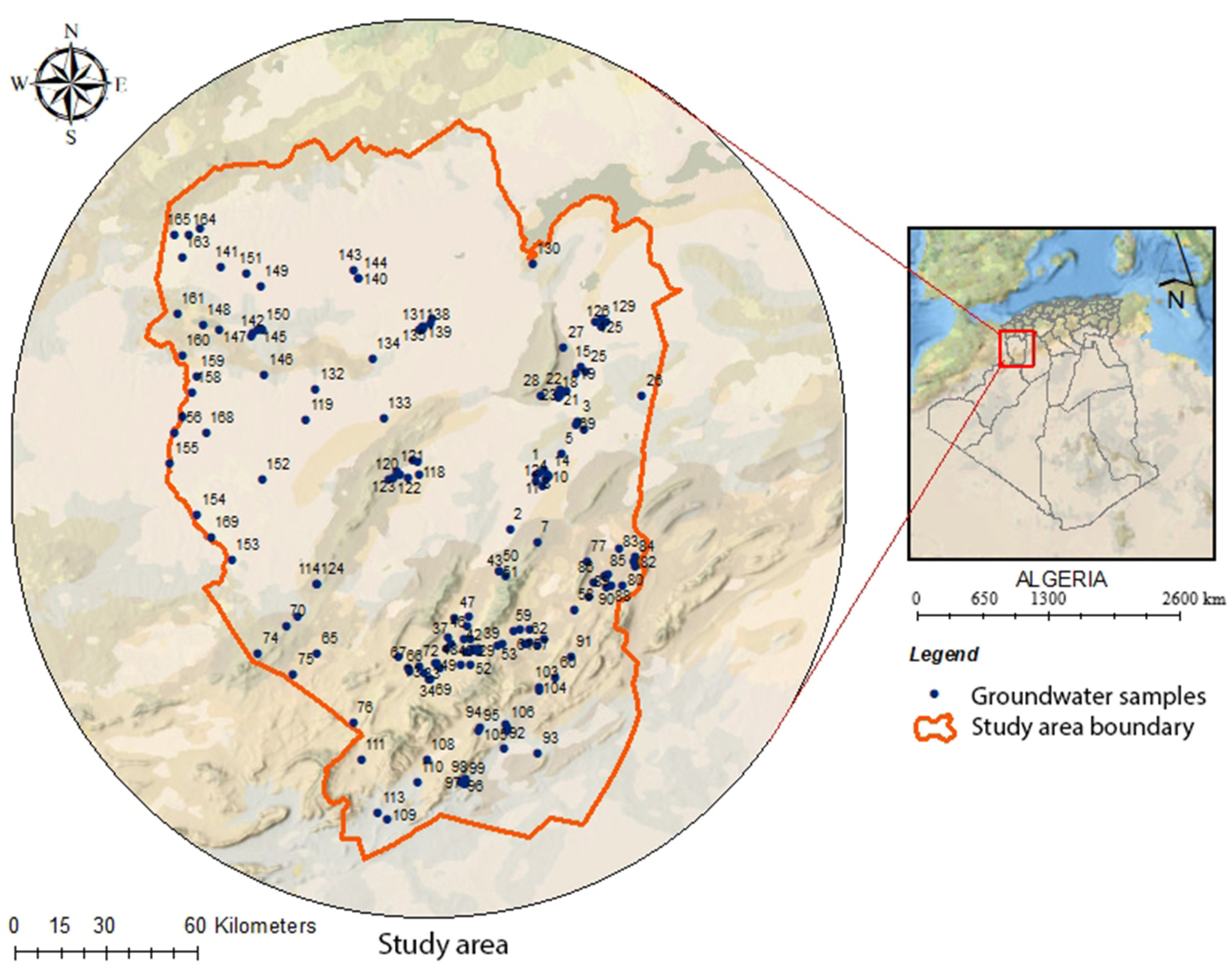
2.1. The Description of the Study Area

We are focusing on the Wilaya of Naama (29,514.14 km2) located in southwestern Algeria, between the latitudes of 33°22′7.84″ N and 33°22′7.84″ N and longitudes 0°21′25.05″ E and 0°21′25.05″ E (Figure 1). The study area’s northern boundary is Wilaya of Tlemcen and Sidi Belabbes, west of the Algerian–Moroccan border, east of Wilaya of El-Bayadh, and south of Wilaya of Bechar. In terms of agricultural activities, the northern section of this research region is marked by pastoral activities and livestock, occupying about 74% of the total area. At the same time, the southern part is characterized by small-scale irrigation systems, with the cultivation of vegetables, cereal, and olive trees [36]. The primary water resources refer to groundwater with four principal aquifer systems: the quaternary alluvial aquifer, the tertiary limestones aquifer, the Jurassic sandstone reservoir, and the Albian aquifer. Among these, the flow rates vary between 5 and 80 L/s. These aquifers provide water for 1,893,122 animals grazing in the study area and 208,136 residents living there [37]. This region’s surface water resources are severely stressed due to climatic conditions [38]. The research area is an arid region with a mean annual rainfall of 287 mm and a maximum yearly rate of evapotranspiration of 2000 mm [39]. Mineral soils, saline soils, and limestone magnetic soils make up the majority of the soil types in this region [40]. According to a land use analysis, the research area’s surface comprises 29.14% steppe ranges, 24.06% severely degraded ranges, 17.94% wind accumulations, only 6.74% dunes, 15.06% rocky outcrops, and 7.05% of forests [41]. Geologically, the tertiary sediments cover the study’s northern area, while the south is composed of cretaceous and Jurassic sediments [42]. The first important economic sector in the wilaya of Naama is agriculture, specifically pastoralism, with more than 2,203,460 Ha of the agricultural area, of which 28,283 Ha is irrigated [43]. The main crops cultivated are cereals and market gardening. All the efforts made by the state contribute to the consolidation of the various actions included in the framework of the national FNRDA program and the upgrading of all the farms on the one hand, and on the other hand, the increase in the area useful as agricultural land through the development of new lands. The main objective is the intensification of agricultural pockets by tree planting as a means of combating desertification and the promotion of fodder crops to meet the needs of livestock.

2.2. Collection of Data, Analysis, and Calculation

From the study area, 166 samples were collected, and ten elements were evaluated (Ca2+, K+, Na+, Mg2+, Cl, NO3, SO42−, HCO3, Electrical Conductivity, and Hydrogen power (pH). A multiparameter portable quality type HANNA (HI98194) was utilized to assess Hydrogen power (pH), Electric Conductivity (EC), and temperature (T) in situ. To evaluate the cation and anion elements, samples were collected and transported to the Sustainable Management of Natural Resources laboratory in Arid and Semi-Arid Zones at Naama and reserved at four degrees Celcius. The chemical analyses were completed using the procedures for the chemical examination of wastes and water (EPA-600/4-79-020) [44]. Magnesium (Mg), Calcium (Ca), and Bicarbonate (HCO3) were evaluated using the method of titration. Atomic absorption spectrometry was used to determine sodium (Na) and potassium (K). Chloride (Cl) concentrations were dosed by the Mohr method. In addition to sulphate (SO4), Nitrate (NO3) was also differentiated by the UV-Vis spectrophotometer. The assessment of the suitability of groundwater in the Naama region for irrigation was established with the international standard (FAO).

2.3. Suitability Indices for Irrigation

Various groundwater indices are frequently used to evaluate groundwater suitability for agricultural use. Sodium percentage, sodium adsorption ratio, Magnesium hazard, Permeability Index, Potential salinity, and Kelly’s ratio. The conventional formulas from (1) to (6), shown in Table 1, were used to determine the (SAR), (MH), (Na%), (PI), (KR), and (PS) correspondingly, where all ions are given in meq/L.

2.4. Irrigation Water Quality Index (IWQI)

It is recognized that the quality of irrigation water and many other factors, such as the nature of the soil, the type of crops, the climatic conditions, and the methods of irrigation, play a significant role in profitability and agricultural yield. The increase in the salinity of irrigation water negatively affects the soil and the plants. The mineral salts present in the irrigation water can cause changes in the structure of the soil, thus modifying its permeability and aeration, which leads to a disturbance in the development of plants [48]. To obtain a clear view of the overall quality of irrigation water, the IWQI was employed to reflect the composite influence of numerous water quality parameters on that water’s overall quality [33,34]. Equation (7) is used in this model to calculate the irrigation water quality parameter (qi), which is determined by the tolerance limits of the parameters listed in Table 2:
q i = q i max x i j x inf × q i a m p X a m p
where q i is the quality of each parameter, q i m a x stands for the maximum value of qi for every class, x i j stands for every parameter’s observed value, and x i n f stands for the value corresponding to the parameter’s lower limit class and where q i a m p   i s   t h e amplitude of quality measurement class, and X a m p is the amplitude class.
Finally, using Equation (8), the IWQI was calculated. Table 3 presents the relative weight of every parameter according to Meireles et al. [32].
I W Q I = i = 1 n q i w i
The IWQI ranges between 0 and 100. Five (05) categories were used to classify the irrigation water quality index IWQI from excellent to inappropriate, as shown in Table 4.

2.5. Extreme Gradient Boosting (XGBoost) Algorithm

XGBoost, which stands for Extreme Gradient Boosting, is a powerful and popular machine learning algorithm that is primarily used for supervised learning tasks, including classification and regression [49,50,51]. It was introduced by Tianqi Chen, a computer scientist and machine learning researcher, in a research paper [52]. XGBoost is an ensemble learning method, meaning it combines the predictions from multiple models (usually decision trees) to create a more robust model. An overview of XGBoost’s work was summarised as follows:
  • Gradient Boosting: XGBoost is a gradient boosting algorithm, which means it combines multiple decision trees to create a stronger predictive model.
  • Decision Trees as Base Learners: Decision trees are used as the base or “weak” learners in XGBoost. These trees are trained to minimize a specified loss function (e.g., mean squared error for regression or log-loss for classification).
  • Iterative Training: XGBoost iteratively adds trees to the model. It starts with an initial prediction (e.g., the mean of the target variable) and then fits a tree to the residuals (the differences between predictions and actual values).
  • Regularization: XGBoost includes regularization techniques (L1 and L2 regularization) to control overfitting and enhance model generalization.
  • Ensemble Learning: The predictions from multiple trees are combined to create the final model. Each new tree is weighted and added to the previous predictions.
  • Parallel and Distributed Computing: XGBoost is designed for efficiency and can leverage parallel and distributed computing to handle large datasets and complex models.
  • Feature Importance: XGBoost provides feature importance scores, helping identify the most influential features in the model’s decisions.
  • Hyperparameter Tuning: To optimize model performance, users can fine-tune hyperparameters like learning rate, tree depth, and subsampling.

2.6. Support Vector Regression (SVR) Algorithm

SVR is a machine learning technique used for regression tasks. It is a variation of the Support Vector Machine (SVM) algorithm primarily used for classification. The second objective of SVR is to predict a continuous target variable (real numbers) based on input features [53,54,55]. First developed by Vladimir N. Vapnik and Alexey Ya Chervonenkis [56], the SVR is used when you have data that do not necessarily follow a linear pattern and may involve complex relationships.
SVR introduces the concept of a margin of tolerance (ε) around the predicted hyperplane. The margin represents the acceptable prediction error, where data points outside this margin contribute to the loss function. SVR seeks to minimize this loss while respecting the margin constraints to find a hyperplane that best fits the data. Support vectors are the data points closest to the margin (inside or on the margin boundary), where these points are the most influential data points, as they have the largest impact on defining the hyperplane [57]. SVR uses a loss function that captures the trade-off between minimizing the error (the difference between simulated and observed values) and maximizing the margin around the hyperplane. The loss function typically has two terms: minimizing the error and controlling the margin. The radial basis function (RBF) is the most common kernel function used to transform the input data into a higher-dimensional space [58].
It controls the trade-off between maintaining a large margin and fitting the data based on regularization parameter, often denoted as “C”. A smaller C value results in a larger margin but may allow more errors, and conversely, training SVR based on Sequential Minimal Optimization (SMO) involves finding the optimal hyperplane and the support vectors. After training, SVR can make predictions for new data points by calculating their position relative to the hyperplane, where the predicted value is influenced by the position and distance from the hyperplane and the margin [59].

2.7. K-Nearest Neighbours (KNN) Algorithm

KNN is a simple yet effective supervised machine learning algorithm for classification and regression tasks. KNN is a non-parametric, instance-based algorithm, meaning it does not make any underlying assumptions about the data distribution and instead relies on the data itself to make predictions. The prediction process in KNN is briefly explained. It mentions that the prediction for a given sample is based on information from its K-Nearest Neighbours in the feature space. K represents the number of neighbours considered when making predictions [60]. The KNN highlights the importance of choosing an appropriate value for k. It is emphasized that the choice of k should depend on the dataset’s specific characteristics and the desired accuracy level. The value of k significantly impacts the algorithm’s performance [61,62].

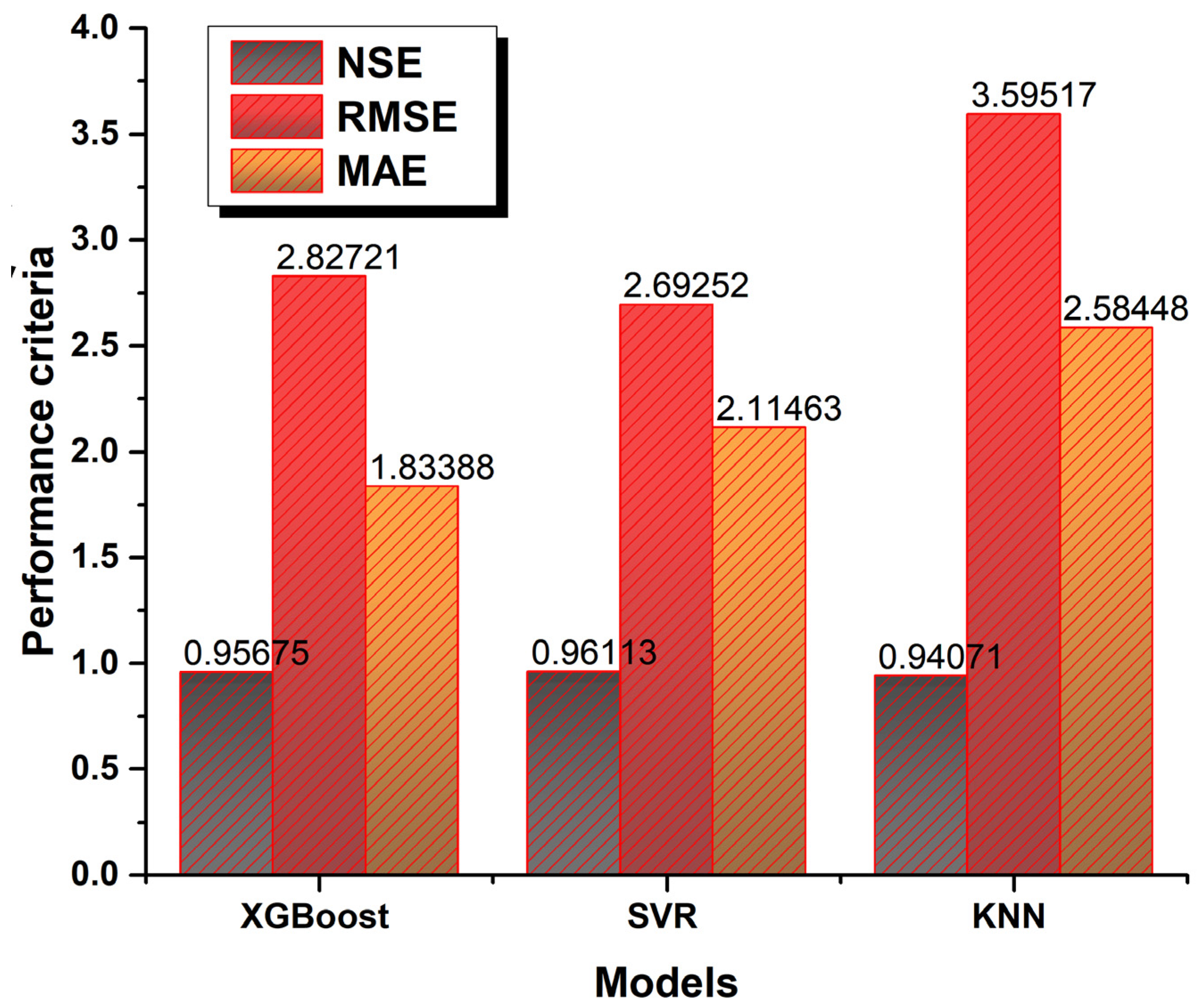
2.8. Performance Criteria

The dataset consisting of 166 samples was divided into separate training and testing subsets to evaluate the proposed algorithms’ effectiveness. The training subset, comprising approximately 70% of the data, equivalent to around 116 samples, was employed for optimizing model parameters and achieving peak performance. The remaining 30% of the data, roughly 50 samples, formed the testing set for conclusive model assessment. This 70/30 data split ratio conforms to a widely recognized practice supported by the existing literature [63,64]. We used multiple performance metrics to assess the model’s effectiveness, including Mean Absolute Error (MAE), Root Mean Square Error (RMSE), Nash–Sutcliffe Efficiency (NSE), and the Pearson Correlation Coefficient (R). Concise explanations of each performance measure are presented below [65,66].
M A E = 1 n i = 1 n I W Q I o , i I W Q I s , i
R M S E = 1 n i = 1 n I W Q I o , i I W Q I s , i 2
N S E = 1 i = 1 n I W Q I o , i I W Q I s , i i = 1 n I W Q I o , i I W Q I o ¯ 2 2
R = i = 1 n I W Q I o , i I W Q I o ¯ I W Q I s , i I W Q I s ¯ i = 1 n I W Q I o b s , i I W Q I o b s ¯ 2 i = 1 n I W Q I s , i I W Q I s ¯ 2
where IWQIo,i and IWQIs,i represent the actual and simulated observations, respectively. N is the sample size of the database. I W Q I o ¯ and I W Q I s ¯ represent the mean values of the actual and simulated samples, respectively.

3. Results

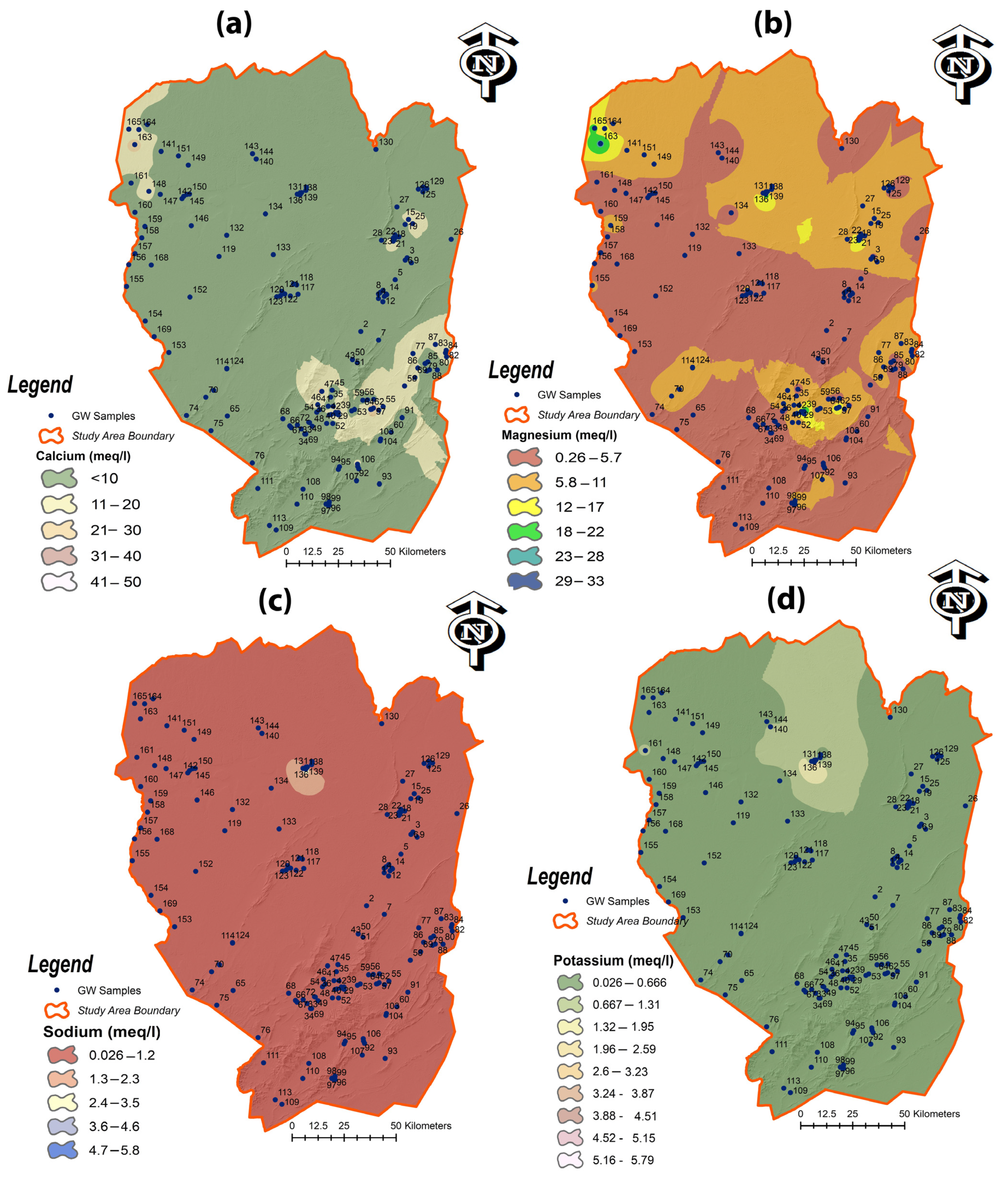
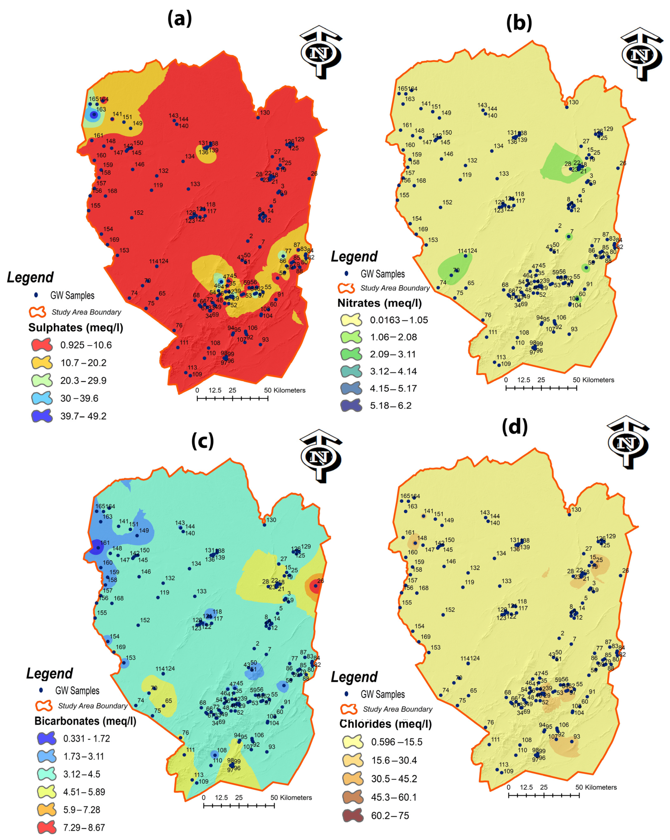
3.1. Descriptive Statistics of Physico-Chemical Parameters of Irrigation Water

Electrical Conductivity (EC), Hydrogen power (pH), main ions ( K + , N a + , C a 2 + , M g + , N O 3 , H C O 3 , S O 4 2 , C l ) are all listed in Table 5, along with their respective minimums, maximums, means, and standard deviations for all 166 samples. The pH of the research area averages at 7.71. Consequently, the groundwater is alkaline in the studied area. Water salinity and total dissolved solids in water can be measured using the practical and trustworthy index of Electrical Conductivity (EC). The values of EC of the study area varied from 290.00 µδ/cm to 6200.00 µδ/cm. According to FAO guidelines, 92.16% of Electrical Conductivity (EC) values of the research area are within an acceptable range (<3000 µδ/cm) [67]. On the other hand, Calcium concentrations in the groundwater of the research area range from 0.60 to 56.10 meq/L (Figure 2a). About 94.6% of the Calcium concentrations are within the permissible range of the FAO recommendations, which set a maximum value of 20 meq/L [67]. While 53.61% of Magnesium concentrations are within the FAO guidelines, as shown in Figure 2b (<5 meq/L) [67]. All sodium results (except only three samples) are within FAO standard limits (<40 meq/L), as these levels varied from 0.22 mg/L to 48.48 mg/L [67]. Among the water sampling points in our study area, potassium values range from 0.03 to 6.69 meq/L (Figure 2d), and the maximum concentration allowed in irrigation water stipulated by FAO is 2.00 meq/L [67]. As a result, all potassium results are within FAO standard limits (except one sample). The mean sulphate value in this study is 7.64 meq/L, ranging from 0.79 to 49.38 meq/L (Figure 3a). One hundred fifty samples of sulphate concentrations are within the guideline range established by the FAO (20 meq/L) [67]. The mean Nitrate concentration ranges between 0.02 and 6.29 meq/L in the groundwater samples (Figure 3b), with a mean value of 0.44 meq/L. Bicarbonate concentrations range from 0.33 to 8.67 meq/L (Figure 3c). We remark that all samples fall within the FAO’s permitted range, with a maximum value of 10 meq/L [67]. Our study region’s average chloride concentration ranges from 0.28 to 79.41 meq/L (Figure 3d). According to FAO guidelines, 94% of chloride values of the research area are within an acceptable range (<30 meq/L) [67].
The irrigation water’s qualitative parameters like Magnesium hazard (MH), sodium percentage ( N a % ), sodium adsorption ratio ( S A R ), Permeability Index ( P I ), Potential salinity ( P S ), and Kelly’s ratio ( K R ) are also reported in Table 3. The values of the sodium adsorption ratio ( S A R ) ranged from 0.12 to 14.56. SAR values between 0 and 18 placed all samples in excellent and good irrigation categories. SAR findings indicate that 98.8% of these samples are excellent and suitable for irrigation (Table 6). As a result of SAR analysis, the irrigation water quality can be classified into four primary categories: “excellent” for water with SARs less than ten meq/L, “good” for water with SARs between 10 and 18 meq/L, “doubtful” for water with SARs between 18 and 26 meq/L, and “unsuitable” for water with SARs more than 26 meq/L. The calculated values for sodium percentage (Na%) spanned from 6.78 to 83.35%. The percent sodium index increases the “permissible” category of the samples to 15.66% while 4.82% are doubtful for irrigation, and decreases the excellent category to 32.53% compared to the SAR classification. According to Aravinthasamy et al. [68], a greater sodium concentration (>60%) may cause the deterioration of the physical properties of soil. It is possible to determine the suitability of groundwater for irrigation based on its Permeability Index (PI) values. PI values, on the other hand, range from 13.41 to 99.07 meq/L, with a mean value of 43.77 meq/L. According to Doneen [47], there are three different categories for the Permeability Index (PI): Class 1, acceptable when PI > 75; Class 2, which is good when PI is between 25 and 75%; and Class 3, which is unsuitable when PI < 25%). It is advised to use water under classes I and II for irrigation [47]. Only 3.61% of the samples in our study area have PI values greater than 25, making them unsuitable for irrigation. As shown in Table 6, all other samples are appropriate for irrigation according to Permeability Index Classification. The Magnesium hazard computed values range from 2.86 to 91.74%. It is not advised to use water for irrigation when the Magnesium hazard value is superior to 50 [45]. Moreover, 46.99% of the samples in the area under study have Magnesium hazard values higher than 50%, making them unsuitable for irrigation (Table 6). It is considered appropriate to irrigate water with a Kelly’s index of less than one due to the assumption that water with a Kelly’s index greater than one contains excessive sodium [46]. The values of KI vary between 0.03 and 4.94, with an average of 0.50. As shown in Table 6, 89.16% of groundwater samples in the study area were suitable for irrigation based on Kelly’s ratio. The values of the Potential salinity of the study area ranged from 1.35 to 83.47 meq/L, while the average value was 10.34 meq/L. Potential salinity (PS) results revealed that 43.98% of samples are “excellent” to “good” for irrigation, 24.10% of samples are “Good” to “Injurious”, and 31.93% are “Injurious” to “Unsatisfactory” for irrigation.

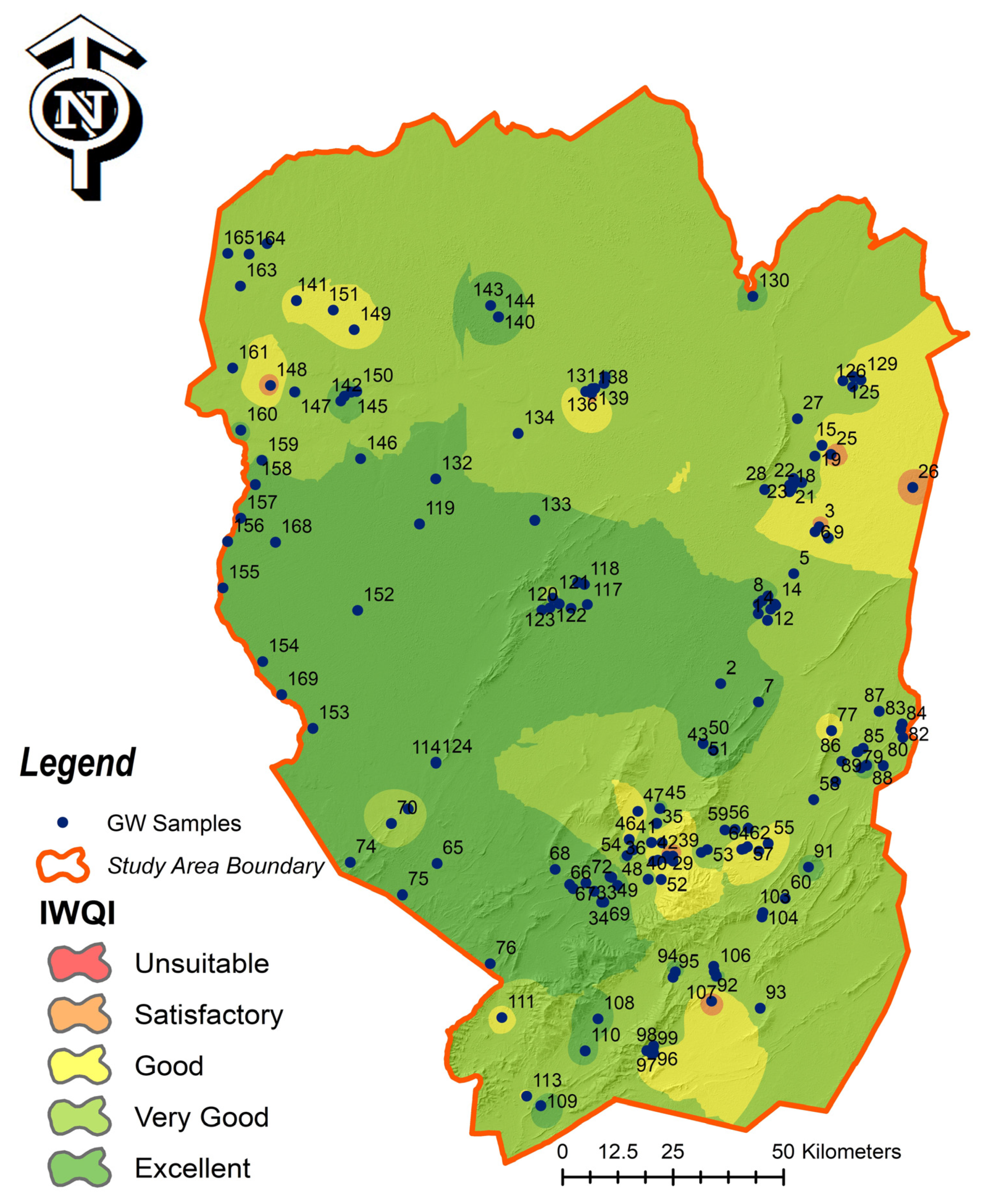
3.2. Irrigation Water Quality Index Assessments

Table 7 shows the IWQI results for the groundwater samples of the Wilaya of Naama. Among the IWQI values, there was a wide range of values, ranging from 1.81 to 97.64, with an average value of 78.15. It has been concluded that the 75 samples falling into the excellent category represent 45.18% of the total samples (Figure 4). About 34.34% of samples fell into the very good category, and 6.63% fell into the good category. A total of 16 samples fall into the satisfactory category, representing 9.64% of the total samples. Meanwhile, the IWQI in seven samples in the study area was characterized as unsuitable for irrigation.

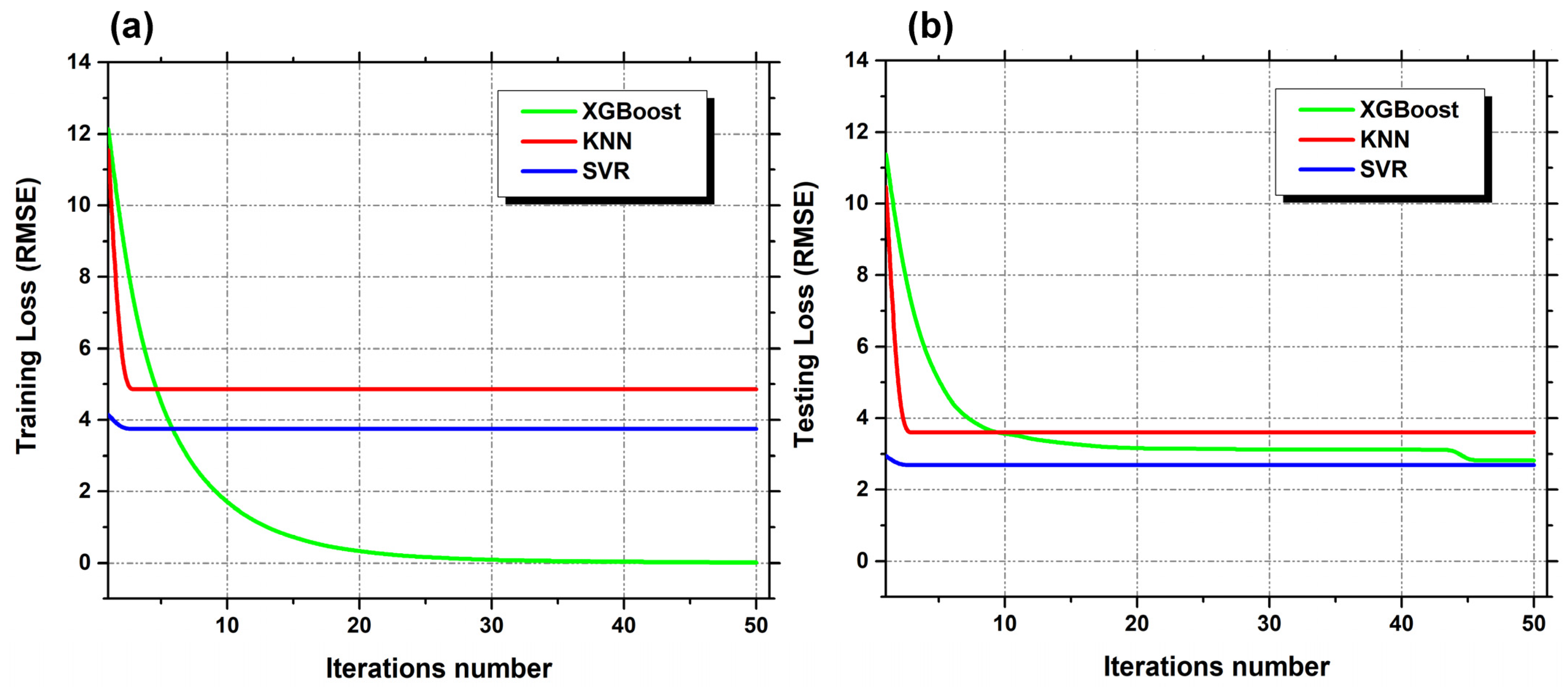
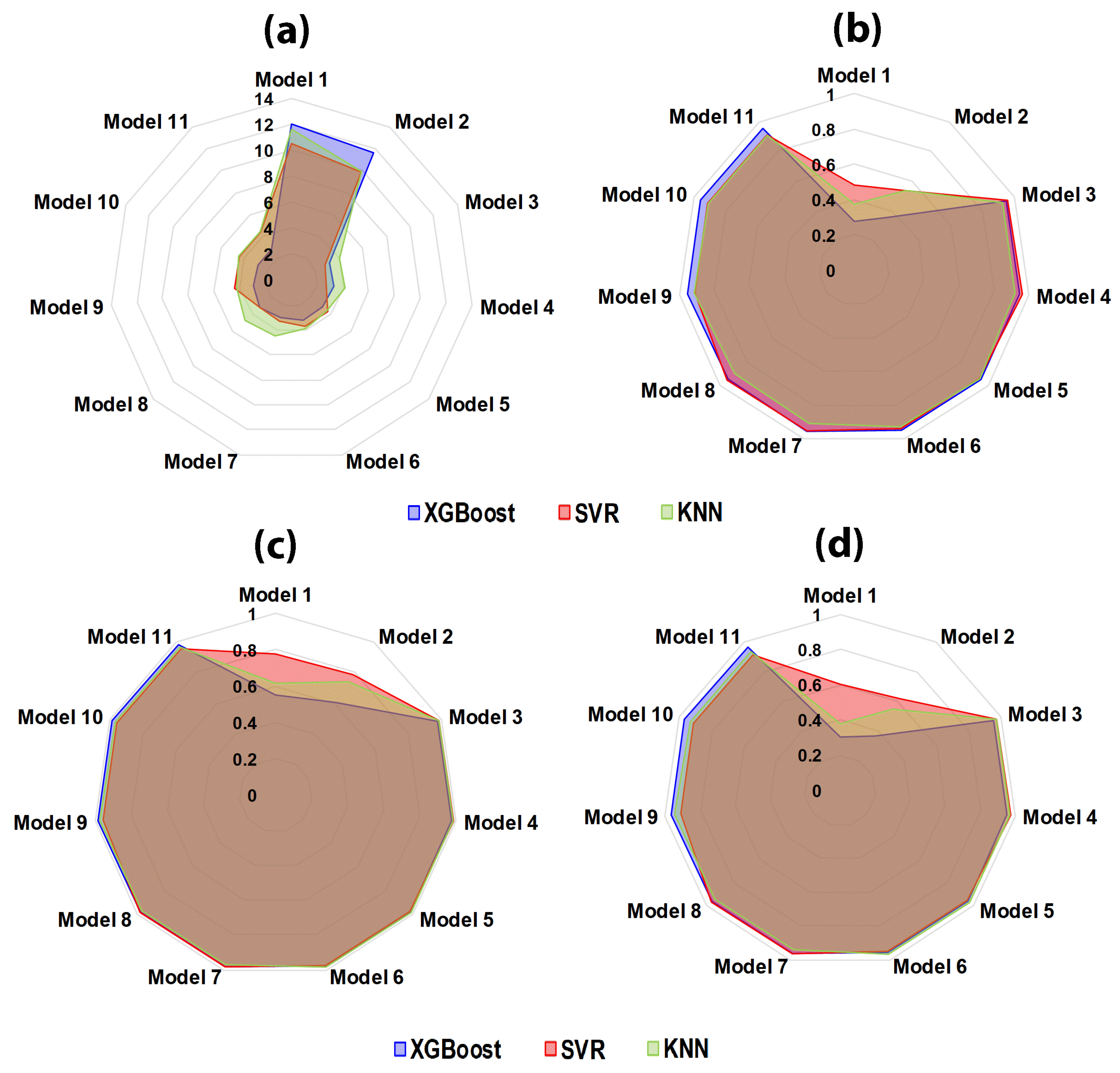
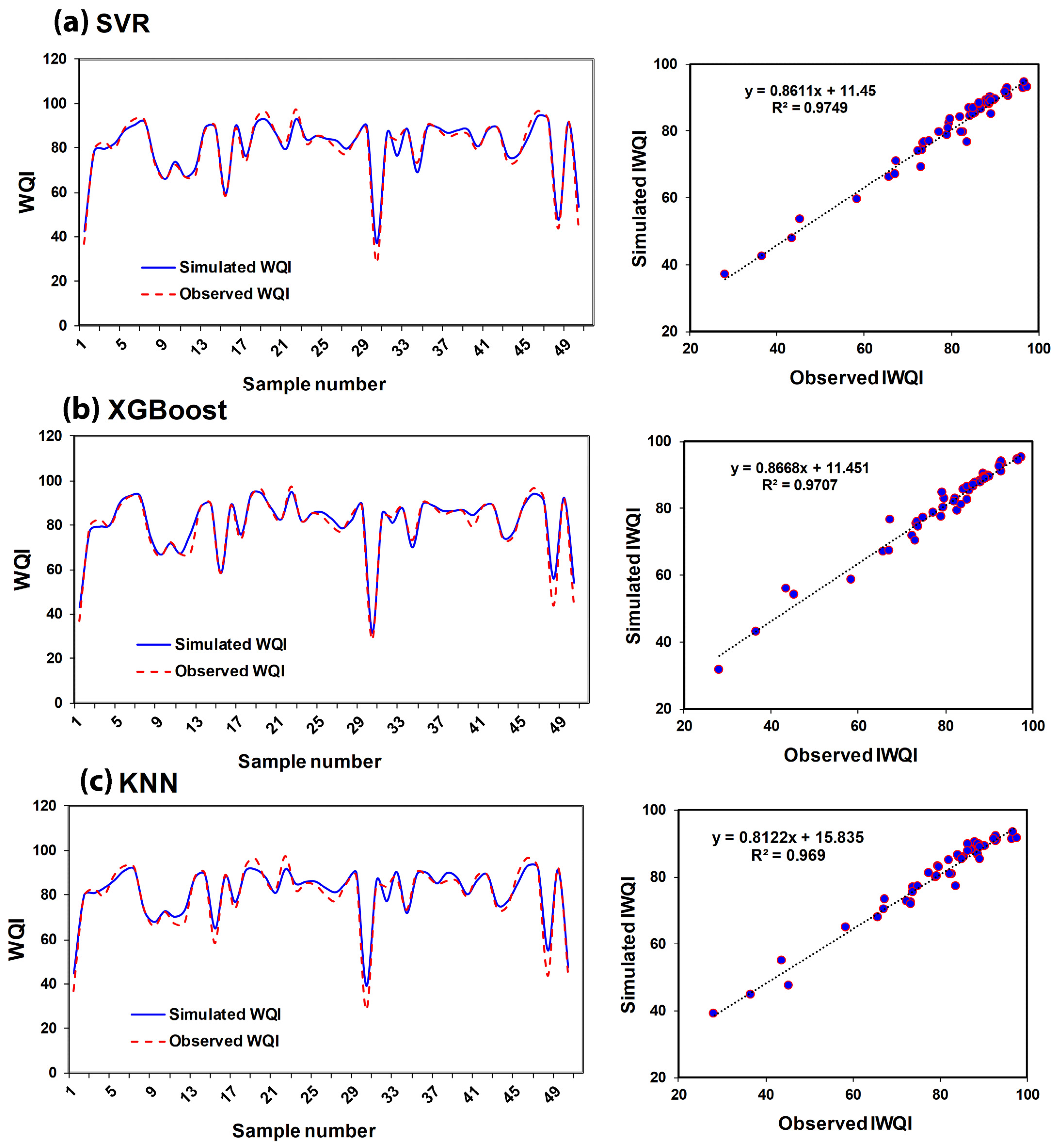
3.3. Machine Learning Analysis and Modelling

A total of 166 data samples of five quality parameters and their actual outputs were used to train three machine learning models: XGBoost, SVR, and KNN algorithms. The input parameters are Ca2+, Mg2+, Na+, K+, Cl, SO42−, HCO3, NO3, EC, Mineralisation, and PH, and IWQI is the output response. The 166 data samples were categorized into five categories expressing irrigation water quality: excellent, very good, good, satisfactory, and unsuitable. Table 8 shows the IWQI status distribution.
Before performing the analysis, eleven input combinations (models) were proposed and assessed based on five performance criteria.
-
Model 1: Ca2+;
-
Model 2: Ca2+, and Mg2+;
-
Model 3: Ca2+, Mg2+, and Na+;
-
Model 4: Ca2+, Mg2+, Na+, and K+;
-
Model 5: Ca2+, Mg2+, Na+, K+, and Cl;
-
Model 6: Ca2+, Mg2+, Na+, K+, Cl, and SO42−;
-
Model 7: Ca2+, Mg2+, Na+, K+, Cl, SO42−, and HCO3;
-
Model 8: Ca2+, Mg2+, Na+, K+, Cl, SO42−, HCO3, and NO3;
-
Model 9: Ca2+, Mg2+, Na+, K+, Cl, SO42−, HCO3, NO3, and EC;
-
Model 10: Ca2+, Mg2+, Na+, K+, Cl, SO42−, HCO3, NO3, EC, and Mineralisation;
-
Model 11: Ca2+, Mg2+, Na+, K+, Cl, SO4−−, HCO3, NO3, EC, Mineralisation, and PH.
The models XGBoost, SVR, and KNN have been implanted using Python programming, which iteratively performs training and testing with the specified applied data. Figure 5 shows the performance of the XGBoost, SVR, and KNN models. The RMSE decreased after the second epochs for SVR and KNN, reaching 4.852 and 3.745 for training and 3.595 and 2.692 for testing, respectively, where the RMSE of XGBoost continued to decrease for both training and validation to epochs or an iteration number of 45, giving its minimum 0.00089029 in training and 2.8272 in testing. Therefore, the best network performance can be considered when the validation error is the lowest.
The training, testing, and validation curves were reduced, as in Figure 5, and the errors decreased, indicating that the XGBoost, SVR, and KNN models are reliable. It is important to know how the three models identify the quality parameters and the output response relationship (IWQI), as well as what the accuracy of the prediction model to obtain the correct prediction of IWQI with the variation of the quality inputs is.
This section presents the results of the analytical investigation. In initial assessments, we measured the effectiveness of basic models using RMSE and NSE as the evaluation metrics. Figure 6 illustrates the comparative RMSE and NSE values for the XGBoost, SVR, and KNN models during the testing phase. Among the 11 models analysed, several models stand out as top performers. Model 7 of XGBoost exhibits the best predictive performance with an impressively low RMSE of 2.99 and the highest NSE of 0.954, demonstrating exceptional accuracy and goodness of fit. Additionally, XGBoost models 9 (Ca2+, Mg2+, Na+, K+, Cl, SO42, HCO3, NO3, and EC) and 10 (Ca2+, Mg2+, Na+, K+, Cl, SO42, HCO3, NO3, and EC) also showcase strong performance, boasting low RMSE values of 2.96 and 2.83, along with high NSE values of 0.953 and 0.957, respectively. Model 4 (Ca2+, Mg2+, Na+, and K+) of SVR is another standout, featuring an RMSE of 2.69 and an exceptional NSE of 0.961, making it one of the top-performing models in the SVR category. In contrast, the SVR model 1 ranks as the least accurate among the models, with an RMSE of 10.52 and an NSE of 0.483, indicating moderate predictive performance. Similarly, SVR models 9 and 10 also exhibit lower predictive performance with RMSE values of 4.42 and 4.39, accompanied by NSE values of 0.911 and 0.912, respectively. When selecting a model, it is crucial to prioritize predictive accuracy, and in this context, the XGBoost models, particularly model 7 and SVR model 4, emerge as the top choices, while SVR model 1 may require further improvement to achieve better results. When selecting a model, it is crucial to prioritize predictive accuracy, and in this context, XGBoost model 10, KNN model 5 (Ca2+, Mg2+, Na+, K+, and Cl), and other high-performing models are excellent choices, while other models may require further improvement to achieve better results.
In this comprehensive analysis, we have assessed the performance of 11 models across three machine learning algorithms, XGBoost, SVR, and KNN, based on R and R2, to gauge their predictive accuracy, goodness of fit, and overall performance (Figure 6).
XGBoost model 10: Among the XGBoost models, model 10 emerges as the top choice. It not only demonstrated the lowest RMSE but also excelled in other metrics, including NSE, R, and R2. With an R2 value of 0.971, this model showcases exceptional predictive capabilities. Its consistently high rankings across multiple metrics underscore its robustness, making it an excellent candidate for accurate predictions. KNN model 3 and KNN model 4: The KNN models, represented by models 3 and 4, also stand out as top-performing models. Both models exhibited R2 values of 0.971 and 0.970, indicating strong predictive accuracy and goodness of fit. These models consistently outperformed other KNN models and demonstrated competitive performance across various metrics. Within the SVR models, model 4 displays noteworthy performance. With an R2 value of 0.975, it exhibits a high level of predictive accuracy and goodness of fit. This model is a strong contender among the SVR models, showcasing its ability to provide reliable predictions. In conclusion, the choice of the best model depends on the specific project requirements. XGBoost model 10 and SVR model 4 are top contenders for tasks demanding the utmost accuracy and goodness of fit. KNN models 3 and 4 offer competitive performance and may be preferred for their simplicity and interpretability
Figure 7 provides a comprehensive comparative analysis of the best-performing models, specifically XGBoost model 10, SVR model 4, and KNN model 5, based on essential evaluation metrics. This figure serves as a visual representation of the model’s predictive capabilities and their suitability for different application scenarios.
In the graph, we observe that XGBoost model 10 stands out with the highest Nash–Sutcliffe Efficiency (NSE) of 0.957, emphasizing its superior predictive accuracy. This model also demonstrates the lowest Root Mean Square Error (RMSE) of 2.827 and an MAE of 1.834, indicating its ability to minimize prediction errors effectively. SVR model 4 maintains strong performance, with an NSE of 0.961 and competitive error measures, including an RMSE of 2.693 and an MAE of 2.115. This model strikes a balance between accuracy and goodness of fit. KNN model 5 highlights robust predictive capabilities with an NSE of 0.941, although it incurs a slightly higher RMSE of 3.595 and an MAE of 2.584. It offers a reliable option with a focus on simplicity.
Figure 8 indicates the correlation between the actual and predicted IWQI output using (a) SVR (model 4), (b) XGBoost (model 10), and (c) KNN (model 5). When comparing the input data of each model within the context of making predictions with limited data, several considerations come into play. The ability to generate accurate predictions with limited data is crucial, and it often depends on the complexity and adaptability of the model. Here is a comparison of the input data for each of the best models, considering their suitability for such scenarios:
When addressing the challenge of making predictions with limited data, the selection of the right modelling approach and input variables becomes pivotal. In this regard, the three best models, XGBoost model 10, SVR model 4, and KNN model 5, each offer unique advantages. XGBoost, represented by model 10, is renowned for its adaptability and robust predictive capabilities. With a comprehensive set of input variables, it can effectively handle sparse datasets. However, success hinges on careful feature selection and parameter tuning to avoid overfitting. In contrast, SVR model 4, with its focused input variables, provides a simpler yet robust solution. Its reduced risk of over-parameterization makes it well-suited for limited data scenarios. KNN model 5, known for its simplicity and adaptability, relies on nearest neighbours and can perform effectively even when data are scarce.
Figure 9 compares the statistical parameters of observed and prediction values based on mean, minimum, maximum, variance, and standard deviation (STD). Mean: All three models have means that are very close to or slightly higher than the reference mean, indicating that they capture the central tendency of the data well. For instance, the mean of XGBoost’s predictions (80.80293) is just slightly higher than the reference (80.01060). Min and Max: The minimum and maximum values of the predicted data by each model are generally within or near the range of the observed data. For example, KNN’s minimum value (39.16076) and maximum value (83.10271) are well within the observed data range. The variance of the predicted data by all three models is lower than the variance of the observed data, indicating that the models provide predictions with reduced variability. For instance, XGBoost and SVR have lower variances compared to the reference data. The STD of the predicted data by each model is also lower than the standard deviation of the observed data, indicating that the models offer predictions with less spread and are less variable than the observed data. XGBoost and SVR have lower standard deviations compared to the reference data.

4. Discussion

In the discussion section, we have comprehensively evaluated the performance of three predictive models, XGBoost (model 10), SVR (model 4), and KNN (model 5), through a range of performance metrics and statistical parameters. XGBoost exhibited strong predictive accuracy with high NSE, low RMSE, and MAE values, closely aligning with the reference data’s central tendency and demonstrating stability with lower variance and standard deviation. SVR showcased notable predictive capability, maintaining a high NSE and low RMSE (2.692) and MAE (2.1146) values, in addition to closely matching the reference data’s central tendency and offering stable and consistent predictions. KNN, while having slightly lower R and R2 values, presented strong predictive performance with a closely aligned central tendency and stable, less variable predictions supported by a lower variance and standard deviation. These findings collectively highlight the models’ potential for accurate, stable, and consistent predictions across various applications. The choice of the best model should be influenced by specific application requirements and priorities, taking into account predictive accuracy, model complexity, and stability. The results obtained from this study agree with research studies that have applied similar approaches for IWQI, which indicated the high performance and stability of machine learning models for IWQI prediction [35,69,70,71]. Lap et al. [72] indicated that the random forest (RF) model excels in accurately forecasting WQI values for the An Hai irrigation system in Vietnam, achieving a good Similarity score of 0.94. This analysis identifies four crucial parameters—Coliform, Dissolved Oxygen (DO), Turbidity, and Total Suspended Solids (TSS)—that exert the most significant influence on water quality. In El Kharga Oasis in the Western Desert of Egypt, Ibrahim et al. [73] found that both the ANFIS and SVM models demonstrated the capability to accurately simulate IWQIs, as evidenced by high determination coefficients (R2) in both the training phase (R2 = 0.99 and 0.97) and the testing phase (R2 = 0.97 and 0.76). In a study by Nguyen et al. [74] for WQI calculations in the Red River Delta, Vietnam, two types of machine learning models were employed. The results revealed that the machine learning model outperformed the deep learning model in terms of prediction accuracy, where the gradient boosting model demonstrated the highest level of predictive accuracy, followed by the XGBoost, RNN, and LSTM models. The accuracy of each of these models was notably high, with predictions ranging from 84% to 96%. Trabelsi and Bel Hadj Ali [75] applied RF, SVR, ANN, and AdaBoost for predicting IWQI in the downstream Medjerda river basin in Tunisia. The findings indicate that the AdaBoost model stands out as the most suitable choice for predicting all parameters, with correlation coefficients (r) ranging between 0.88 and 0.89. On the other hand, the random forest model is well-suited for predicting four specific parameters, namely TDS, SAR, PS, and ESP, with R in the range of 0.65 to 0.87.
Finally, despite the uncertainty and limitations of machine learning algorithms, these results highlight the potential of XGBoost, SVR, and KNN as valuable tools for groundwater quality prediction. They can provide essential insights and serve as a basis for further research and monitoring. However, their utility should be complemented by expert knowledge and traditional hydrogeological methods for more robust decision-making and practical applications. Finally, this section emphasizes the need for further research to validate the models under different data conditions, including more dispersed groundwater quality data. We also highlight potential avenues for future research aimed at refining the models in response to varying data characteristics.

5. Conclusions

Arid and semi-arid regions often rely solely on groundwater for irrigation. The management of water resources for drinking and irrigation can be enhanced by understanding and evaluating the irrigation water quality index. Based on data collected from 166 boreholes in Naama, located in southwestern Algeria, the study aims to determine the irrigation water quality index (IWQI), which consists of many physico-chemical parameters. Furthermore, this research rigorously evaluated three predictive models, namely XGBoost, SVR, and KNN, for estimating the IWQI variable. The models were thoroughly assessed using multiple performance metrics, including NSE, RMSE, MAE, R.
The results of the irrigation water qualitative parameter analysis of the groundwater samples of the study area revealed that most of them were “suitable.” Based on the findings of IWQI, we found that 45.18% of samples were categorized as “excellent”, 34.34% of samples were considered as “very good”, 6.63% of samples fell into the good category, 9.64% of the total samples were categorized as “satisfactory”, and 4.21% of samples in the study area were characterized as “unsuitable” of irrigation.
In IWQI modelling, XGBoost (model 10) emerged as a strong performer, with high NSE and low RMSE and MAE values, signifying its predictive accuracy. It is closely aligned with the reference data in terms of mean, minimum, and maximum predictions while offering reduced variability.
SVR (model 4) demonstrated a notable predictive capability, boasting high NSE (0.96112) and low RMSE (2.6925) and MAE (2.11462) values. It closely matched the reference data’s mean and exhibited consistent predictions within the observed data range. Lower variance and standard deviation values emphasized its stability. We found four important parameters that have the greatest impact on water quality, including Ca2+, Mg2+, Na+, and K.
KNN (model 5) showcased strong predictive performance with competitive NSE, RMSE, and MAE values. Although it had slightly lower R and R2 values, its predictions closely followed the reference data, with reduced variance and standard deviation, indicating stability.
This study may offer useful and valuable information for decision-makers to comprehend the present state of the water quality for irrigation in the Wilaya of Naama. This will allow for a better and more sustainable management of water resources in the study area and similar regions. Finally, the application of metaheuristic algorithms in conjunction with machine learning is a promising avenue for future research and practical implementations.

Author Contributions

Conceptualization, E.E.H., A.D., B.Z., A.A., M.B.-d.l.S., Y.J.W. and M.A.H.; data curation, E.E.H. and A.D.; formal analysis, E.E.H., A.D., B.Z., M.B.-d.l.S. and A.A.; funding acquisition, A.A.; investigation, E.E.H., A.D., A.A. and M.A.H.; methodology, E.E.H., A.D. and M.A.H.; project administration, E.E.H. and A.D.; resources, E.E.H., A.D., A.E., and A.A.; software, E.E.H., A.D. and B.Z.; supervision, E.E.H., P.M.N., and A.D.; validation, A.E., E.E.H., Y.J.W., A.D., A.A., M.B.-d.l.S. and M.A.H.; visualization, A.A. and P.M.N., A.E., M.A.H.; writing—original draft, E.E.H., A.D., Y.J.W., A.E., and B.Z.; writing—review and editing, E.E.H., A.A., M.B.-d.l.S. and M.A.H. All authors have read and agreed to the published version of the manuscript.

Funding

This work is funded and supported by the Deanship of Scientific Research, Taif University.

Data Availability Statement

The data that support the findings of this study are available on request from the corresponding author, [Y.J.W.].

Acknowledgments

The researchers would like to acknowledge the Deanship of Scientific Research, Taif University, for funding this work.

Conflicts of Interest

The authors declare no conflicts of interest.

References

  1. Gleeson, T.; Alley, W.M.; Allen, D.M.; Sophocleous, M.A.; Zhou, Y.; Taniguchi, M.; VanderSteen, J. Towards sustainable groundwater use: Setting long-term goals, backcasting, and managing adaptively. Groundwater 2012, 50, 19–26. [Google Scholar] [CrossRef]
  2. Laube, W.; Schraven, B.; Awo, M. Smallholder adaptation to climate change: Dynamics and limits in Northern Ghana. Clim. Chang. 2012, 111, 753–774. [Google Scholar] [CrossRef]
  3. Maja, M.M.; Ayano, S.F. The impact of population growth on natural resources and farmers’ capacity to adapt to climate change in low-income countries. Earth Syst. Environ. 2021, 5, 271–283. [Google Scholar] [CrossRef]
  4. Xanke, J.; Liesch, T. Quantification and possible causes of declining groundwater resources in the Euro-Mediterranean region from 2003 to 2020. Hydrogeol. J. 2022, 30, 379–400. [Google Scholar] [CrossRef]
  5. Li, Q.; Lu, L.; Zhao, Q.; Hu, S. Impact of Inorganic Solutes&rsquo; Release in Groundwater during Oil Shale In Situ Exploitation. Water 2023, 15, 172. [Google Scholar] [CrossRef]
  6. Molajou, A.; Afshar, A.; Khosravi, M.; Soleimanian, E.; Vahabzadeh, M.; Variani, H.A. A new paradigm of water, food, and energy nexus. Environ. Sci. Pollut. Res. 2023, 30, 107487–107497. [Google Scholar] [CrossRef]
  7. Mekonnen, M.M.; Gerbens-Leenes, W. The water footprint of global food production. Water 2020, 12, 2696. [Google Scholar] [CrossRef]
  8. Tian, H.; Huang, N.; Niu, Z.; Qin, Y.; Pei, J.; Wang, J. Mapping Winter Crops in China with Multi-Source Satellite Imagery and Phenology-Based Algorithm. Remote Sens. 2019, 11, 820. [Google Scholar] [CrossRef]
  9. Abobatta, W. Impact of hydrogel polymer in agricultural sector. Adv. Agric. Environ. Sci. Open Access 2018, 1, 59–64. [Google Scholar] [CrossRef]
  10. Gerten, D.; Heck, V.; Jägermeyr, J.; Bodirsky, B.L.; Fetzer, I.; Jalava, M.; Kummu, M.; Lucht, W.; Rockström, J.; Schaphoff, S. Feeding ten billion people is possible within four terrestrial planetary boundaries. Nat. Sustain. 2020, 3, 200–208. [Google Scholar] [CrossRef]
  11. Wang, X. Managing Land Carrying Capacity: Key to Achieving Sustainable Production Systems for Food Security. Land 2022, 11, 484. [Google Scholar] [CrossRef]
  12. Abdessamed, D.; Jodar-Abellan, A.; Ghoneim, S.S.M.; Almaliki, A.; Hussein, E.E.; Pardo, M.Á. Groundwater quality assessment for sustainable human consumption in arid areas based on GIS and water quality index in the watershed of Ain Sefra (SW of Algeria). Environ. Earth Sci. 2023, 82, 510. [Google Scholar] [CrossRef]
  13. FAO (Food and Agriculture Organization). AQUASTAT—FAO’s Global Information System on Water and Agriculture. Available online: https://www.fao.org/aquastat/en/geospatial-information/global-maps-irrigated-areas/irrigation-by-country/country/DZA (accessed on 16 October 2023).
  14. Amichi, H.; Bouarfa, S.; Kuper, M.; Ducourtieux, O.; Imache, A.; Fusillier, J.L.; Bazin, G.; Hartani, T.; Chehat, F. How does unequal access to groundwater contribute to marginalization of small farmers? The case of public lands in Algeria. Irrig. Drain. 2012, 61, 34–44. [Google Scholar] [CrossRef]
  15. Hounslow, A.W. Water Quality Data: Analysis and Interpretation; CRC Press: Boca Raton, FL, USA, 2018. [Google Scholar]
  16. Zaman, M.; Shahid, S.A.; Heng, L. Irrigation water quality. In Guideline for Salinity Assessment, Mitigation and Adaptation Using Nuclear and Related Techniques; Springer: Berlin/Heidelberg, Germany, 2018; pp. 113–131. [Google Scholar]
  17. Turdaliev, A.; Darmonov, D.Y.; Teshaboyev, N.; Saminov, A.; Abdurakhmonova, M. Influence of irrigation with salty water on the composition of absorbed bases of hydromorphic structure of soil. IOP Conf. Ser. Earth Environ. Sci. 2022, 1068, 012047. [Google Scholar] [CrossRef]
  18. Tlili-Zrelli, B.; Hamzaoui-Azaza, F.; Gueddari, M.; Bouhlila, R. Geochemistry and quality assessment of groundwater using graphical and multivariate statistical methods. A case study: Grombalia phreatic aquifer (Northeastern Tunisia). Arab. J. Geosci. 2013, 6, 3545–3561. [Google Scholar] [CrossRef]
  19. Nishanthiny, S.C.; Thushyanthy, M.; Barathithasan, T.; Saravanan, S. Irrigation water quality based on hydro chemical analysis, Jaffna, Sri Lanka. Am.-Eurasian J. Agric. Environ. Sci. 2010, 7, 100–102. [Google Scholar]
  20. Cymes, I.; Glińska-Lewczuk, K. The use of water quality indices (WQI and SAR) for multipurpose assessment of water in dam reservoirs. J. Elem. 2016, 21, 1211–1224. [Google Scholar]
  21. Chaganti, V.N.; Crohn, D.M.; Šimůnek, J. Leaching and reclamation of a biochar and compost amended saline–sodic soil with moderate SAR reclaimed water. Agric. Water Manag. 2015, 158, 255–265. [Google Scholar] [CrossRef]
  22. Rengasamy, P. Irrigation water quality and soil structural stability: A perspective with some new insights. Agronomy 2018, 8, 72. [Google Scholar] [CrossRef]
  23. Misaghi, F.; Delgosha, F.; Razzaghmanesh, M.; Myers, B. Introducing a water quality index for assessing water for irrigation purposes: A case study of the Ghezel Ozan River. Sci. Total Environ. 2017, 589, 107–116. [Google Scholar] [CrossRef] [PubMed]
  24. Koklu, R.; Sengorur, B.; Topal, B. Water quality assessment using multivariate statistical methods—A case study: Melen River System (Turkey). Water Resour. Manag. 2010, 24, 959–978. [Google Scholar] [CrossRef]
  25. Zhang, B.; Song, X.; Zhang, Y.; Han, D.; Tang, C.; Yu, Y.; Ma, Y. Hydrochemical characteristics and water quality assessment of surface water and groundwater in Songnen plain, Northeast China. Water Res. 2012, 46, 2737–2748. [Google Scholar] [CrossRef] [PubMed]
  26. Prasanna, M.; Praveena, S.; Chidambaram, S.; Nagarajan, R.; Elayaraja, A. Evaluation of water quality pollution indices for heavy metal contamination monitoring: A case study from Curtin Lake, Miri City, East Malaysia. Environ. Earth Sci. 2012, 67, 1987–2001. [Google Scholar] [CrossRef]
  27. Barakat, A.; El Baghdadi, M.; Rais, J.; Aghezzaf, B.; Slassi, M. Assessment of spatial and seasonal water quality variation of Oum Er Rbia River (Morocco) using multivariate statistical techniques. Int. Soil Water Conserv. Res. 2016, 4, 284–292. [Google Scholar] [CrossRef]
  28. Eaton, F.M. Significance of carbonates in irrigation waters. Soil Sci. 1950, 69, 123–134. [Google Scholar] [CrossRef]
  29. Doneen, L. Notes on Water Quality in Agriculture; Published as a Water Sciences and Engineering; Department of Water Sciences and Engineering, University of California: Davis, CA, USA, 1964; Volume 4001. [Google Scholar]
  30. Brown, R.M.; McClelland, N.I.; Deininger, R.A.; O’Connor, M.F. A water quality index—Crashing the psychological barrier. In Indicators of Environmental Quality; Springer: Berlin/Heidelberg, Germany, 1972; pp. 173–182. [Google Scholar]
  31. Horton, R.K. An index number system for rating water quality. J. Water Pollut. Control. Fed. 1965, 37, 300–306. [Google Scholar]
  32. Meireles, A.C.M.; Andrade, E.M.d.; Chaves, L.C.G.; Frischkorn, H.; Crisostomo, L.A. A new proposal of the classification of irrigation water. Rev. Ciência Agronômica 2010, 41, 349–357. [Google Scholar] [CrossRef]
  33. Şener, Ş.; Varol, S.; Şener, E. Evaluation of sustainable groundwater utilization using index methods (WQI and IWQI), multivariate analysis, and GIS: The case of Akşehir District (Konya/Turkey). Environ. Sci. Pollut. Res. 2021, 28, 47991–48010. [Google Scholar] [CrossRef]
  34. Batarseh, M.; Imreizeeq, E.; Tilev, S.; Al Alaween, M.; Suleiman, W.; Al Remeithi, A.M.; Al Tamimi, M.K.; Al Alawneh, M. Assessment of groundwater quality for irrigation in the arid regions using irrigation water quality index (IWQI) and GIS-Zoning maps: Case study from Abu Dhabi Emirate, UAE. Groundw. Sustain. Dev. 2021, 14, 100611. [Google Scholar] [CrossRef]
  35. El Bilali, A.; Taleb, A. Prediction of irrigation water quality parameters using machine learning models in a semi-arid environment. J. Saudi Soc. Agric. Sci. 2020, 19, 439–451. [Google Scholar] [CrossRef]
  36. Moussaoui, T.; Derdour, A.; Hosni, A.; Ballesta-de los Santos, M.; Legua, P.; Pardo-Picazo, M.Á. Assessing the Quality of Treated Wastewater for Irrigation: A Case Study of Ain Sefra Wastewater Treatment Plant. Sustainability 2023, 15, 11133. [Google Scholar] [CrossRef]
  37. Abdessamed, D.; Abderrazak, B. Coupling HEC-RAS and HEC-HMS in rainfall–runoff modeling and evaluating floodplain inundation maps in arid environments: Case study of Ain Sefra city, Ksour Mountain. SW of Algeria. Environ. Earth Sci. 2019, 78, 586. [Google Scholar] [CrossRef]
  38. Derdour, A.; Abdo, H.G.; Almohamad, H.; Alodah, A.; Al Dughairi, A.A.; Ghoneim, S.S.; Ali, E. Prediction of Groundwater Water Quality Index Using Classification Techniques in Arid Environments. Sustainability 2023, 15, 9687. [Google Scholar] [CrossRef]
  39. Derdour, A.; Bouarfa, S.; Kaid, N.; Baili, J.; Al-Bahrani, M.; Menni, Y.; Ahmad, H. Assessment of the impacts of climate change on drought in an arid area using drought indices and Landsat remote sensing data. Int. J. Low-Carbon Technol. 2022, 17, 1459–1469. [Google Scholar] [CrossRef]
  40. Bouarfa, S.; Derdour, A.; Okkacha, Y.; Almaliki, A.H.; Jodar-Abellan, A.; Hussein, E.E. Sedimentological investigation of the potential origin and provenance of sand deposits in an arid area: A case study of the Ksour Mountains Region in Algeria. Arab. J. Geosci. 2022, 15, 1460. [Google Scholar] [CrossRef]
  41. Derdour, A.; Bouanani, A.; Babahamed, K. Modelling rainfall runoff relations using HEC-HMS in a semi-arid region: Case study in Ain Sefra watershed, Ksour Mountains (SW Algeria). J. Water Land Dev. 2018, 36, 45–55. [Google Scholar] [CrossRef]
  42. Derdour, A.; Benkaddour, Y.; Bendahou, B. Application of remote sensing and GIS to assess groundwater potential in the transboundary watershed of the Chott-El-Gharbi (Algerian–Moroccan border). Appl. Water Sci. 2022, 12, 136. [Google Scholar] [CrossRef]
  43. Lachache, S.; Derdour, A.; Maazouzi, I.; Amroune, A.; Guastaldi, E.; Merzougui, T. Statistical Approach Of Groundwater Quality Assessment At Naama Region, South-West Algeria. LARHYSS J. 2023, 55, 125–145. [Google Scholar]
  44. Khodapanah, L.; Sulaiman, W.; Khodapanah, N. Groundwater quality assessment for different purposes in Eshtehard District, Tehran, Iran. Eur. J. Sci. Res. 2009, 36, 543–553. [Google Scholar] [CrossRef]
  45. Richards, L.A. Diagnosis and Improvement of Saline and Alkali Soils; LWW: Washington, DC, USA, 1954; Volume 78. [Google Scholar]
  46. Kelly, W. Permissible composition and concentration of irrigated waters. Proc. ASCF 1940, 66, 607–613. [Google Scholar]
  47. Wong, Y.J.; Shimizu, Y.; He, K.; Nik Sulaiman, N.M. Comparison among different ASEAN water quality indices for the assessment of the spatial variation of surface water quality in the Selangor river basin, Malaysia. Environ. Monit. Assess 2020, 192, 644. [Google Scholar] [CrossRef] [PubMed]
  48. Doneen, L.D. Salination of soil by salts in the irrigation water. Eos Trans. Am. Geophys. Union 1954, 35, 943–950. [Google Scholar]
  49. Lu, H.; Ma, X. Hybrid decision tree-based machine learning models for short-term water quality prediction. Chemosphere 2020, 249, 126169. [Google Scholar] [CrossRef] [PubMed]
  50. Lee, J.; Lee, J.; Lee, M.; Lee, M.; Kim, Y.; Hyung, J.; Kim, K.; Cha, Y.; Koo, J. Development of a short-term water quality prediction model for urban rivers using real-time water quality data. Water Supply 2022, 22, 4082–4097. [Google Scholar] [CrossRef]
  51. Wong, Y.J.; Nakayama, R.; Shimizu, Y.; Kamiya, A.; Shen, S.; Muhammad Rashid, I.Z.; Nik Sulaiman, N.M. Toward industrial revolution 4.0: Development, validation, and application of 3D-printed IoT-based water quality monitoring system. J. Clean. Prod. 2021, 324, 129230. [Google Scholar] [CrossRef]
  52. Chen, T.; Guestrin, C. Xgboost: A scalable tree boosting system. In Proceedings of the 22nd ACM Sigkdd International Conference on Knowledge Discovery and Data Mining, San Francisco, CA, USA, 13–17 August 2016; pp. 785–794. [Google Scholar]
  53. Wong, Y.J.; Shimizu, Y.; Kamiya, A.; Maneechot, L.; Bharambe, K.P.; Fong, C.S.; Nik Sulaiman, N.M. Application of artificial intelligence methods for monsoonal river classification in Selangor river basin, Malaysia. Environ. Monit. Assess 2021, 193, 438. [Google Scholar] [CrossRef] [PubMed]
  54. Najafzadeh, M.; Niazmardi, S. A novel multiple-kernel support vector regression algorithm for estimation of water quality parameters. Nat. Resour. Res. 2021, 30, 3761–3775. [Google Scholar] [CrossRef]
  55. Su, X.; He, X.; Zhang, G.; Chen, Y.; Li, K. Research on SVR water quality prediction model based on improved sparrow search algorithm. Comput. Intell. Neurosci. 2022, 2022, 7327072. [Google Scholar] [CrossRef]
  56. Vapnik, V. The Nature of Statistical Learning Theory; Springer Science & Business Media: Berlin/Heidelberg, Germany, 1999. [Google Scholar]
  57. Sakaa, B.; Elbeltagi, A.; Boudibi, S.; Chaffaï, H.; Islam, A.R.M.T.; Kulimushi, L.C.; Choudhari, P.; Hani, A.; Brouziyne, Y.; Wong, Y.J. Water quality index modeling using random forest and improved SMO algorithm for support vector machine in Saf-Saf river basin. Environ. Sci. Pollut. Res. 2022, 29, 48491–48508. [Google Scholar] [CrossRef]
  58. Li, J.; Abdulmohsin, H.A.; Hasan, S.S.; Kaiming, L.; Al-Khateeb, B.; Ghareb, M.I.; Mohammed, M.N. Hybrid soft computing approach for determining water quality indicator: Euphrates River. Neural Comput. Appl. 2019, 31, 827–837. [Google Scholar] [CrossRef]
  59. Wang, X.; Zhang, F.; Ding, J. Evaluation of water quality based on a machine learning algorithm and water quality index for the Ebinur Lake Watershed, China. Sci. Rep. 2017, 7, 12858. [Google Scholar] [CrossRef] [PubMed]
  60. Tahraoui, H.; Toumi, S.; Hassein-Bey, A.H.; Bousselma, A.; Sid, A.N.E.H.; Belhadj, A.-E.; Triki, Z.; Kebir, M.; Amrane, A.; Zhang, J. Advancing Water Quality Research: K-Nearest Neighbor Coupled with the Improved Grey Wolf Optimizer Algorithm Model Unveils New Possibilities for Dry Residue Prediction. Water 2023, 15, 2631. [Google Scholar] [CrossRef]
  61. Juna, A.; Umer, M.; Sadiq, S.; Karamti, H.; Eshmawi, A.A.; Mohamed, A.; Ashraf, I. Water quality prediction using KNN imputer and multilayer perceptron. Water 2022, 14, 2592. [Google Scholar] [CrossRef]
  62. Kim, M.; Kim, Y.; Kim, H.; Piao, W.; Kim, C. Evaluation of the k-nearest neighbor method for forecasting the influent characteristics of wastewater treatment plant. Front. Environ. Sci. Eng. 2016, 10, 299–310. [Google Scholar] [CrossRef]
  63. Budiarti, R.P.N.; Sukaridhoto, S.; Hariadi, M.; Purnomo, M.H. Big data technologies using SVM (case study: Surface water classification on regional water utility company in Surabaya). In Proceedings of the 2019 International Conference on Computer Science, Information Technology, and Electrical Engineering (ICOMITEE), Jember, Indonesia, 16–17 October 2019; pp. 94–101. [Google Scholar]
  64. Wong, Y.J.; Arumugasamy, S.K.; Chung, C.H.; Selvarajoo, A.; Sethu, V. Comparative study of artificial neural network (ANN), adaptive neuro-fuzzy inference system (ANFIS) and multiple linear regression (MLR) for modeling of Cu (II) adsorption from aqueous solution using biochar derived from rambutan (Nephelium lappaceum) peel. Environ. Monit. Assess 2020, 192, 439. [Google Scholar] [CrossRef] [PubMed]
  65. Abda, Z.; Zerouali, B.; Alqurashi, M.; Chettih, M.; Santos, C.A.G.; Hussein, E.E. Suspended sediment load simulation during flood events using intelligent systems: A case study on semiarid regions of Mediterranean Basin. Water 2021, 13, 3539. [Google Scholar] [CrossRef]
  66. Zerouali, B.; Santos, C.A.G.; de Farias, C.A.S.; Muniz, R.S.; Difi, S.; Abda, Z.; Chettih, M.; Heddam, S.; Anwar, S.A.; Elbeltagi, A. Artificial intelligent systems optimized by metaheuristic algorithms and teleconnection indices for rainfall modeling: The case of a humid region in the mediterranean basin. Heliyon 2023, 9, e15355. [Google Scholar] [CrossRef]
  67. Ayers, R.S.; Westcot, D.W. Water Quality for Agriculture; Food and Agriculture Organization of the United Nations Rome: Rome, Italy, 1985; Volume 29. [Google Scholar]
  68. Aravinthasamy, P.; Karunanidhi, D.; Subramani, T.; Roy, P.D. Demarcation of groundwater quality domains using GIS for best agricultural practices in the drought-prone Shanmuganadhi River basin of South India. Environ. Sci. Pollut. Res. 2021, 28, 18423–18435. [Google Scholar] [CrossRef]
  69. M’nassri, S.; El Amri, A.; Nasri, N.; Majdoub, R. Estimation of irrigation water quality index in a semi-arid environment using data-driven approach. Water Supply 2022, 22, 5161–5175. [Google Scholar] [CrossRef]
  70. Mokhtar, A.; Elbeltagi, A.; Gyasi-Agyei, Y.; Al-Ansari, N.; Abdel-Fattah, M.K. Prediction of irrigation water quality indices based on machine learning and regression models. Appl. Water Sci. 2022, 12, 76. [Google Scholar] [CrossRef]
  71. Omeka, M.E. Evaluation and prediction of irrigation water quality of an agricultural district, SE Nigeria: An integrated heuristic GIS-based and machine learning approach. Environ. Sci. Pollut. Res. 2023, 1–26. [Google Scholar] [CrossRef] [PubMed]
  72. Lap, B.Q.; Du Nguyen, H.; Hang, P.T.; Phi, N.Q.; Hoang, V.T.; Linh, P.G.; Hang, B.T.T. Predicting water quality index (WQI) by feature selection and machine learning: A case study of An Kim Hai irrigation system. Ecol. Inform. 2023, 74, 101991. [Google Scholar] [CrossRef]
  73. Ibrahim, H.; Yaseen, Z.; Scholz, M.; Ali, M.; Gad, M.; Elsayed, S.; Khadr, M.; Hussein, H.; Ibrahim, H.; Eid, M. Evaluation and prediction of groundwater quality for irrigation using an integrated water quality indices, machine learning models and GIS approaches: A representative case study. Water 2023, 15, 694. [Google Scholar] [CrossRef]
  74. Nguyen, D.P.; Ha, H.D.; Trinh, N.T.; Nguyen, M.T. Application of artificial intelligence for forecasting surface quality index of irrigation systems in the Red River Delta, Vietnam. Environ. Syst. Res. 2023, 12, 24. [Google Scholar] [CrossRef]
  75. Trabelsi, F.; Bel Hadj Ali, S. Exploring machine learning models in predicting irrigation groundwater quality indices for effective decision making in Medjerda River Basin, Tunisia. Sustainability 2022, 14, 2341. [Google Scholar] [CrossRef]
Figure 1. Study area.
Water 16 00264 g001
Figure 2. Geospatial distribution of (a) calcium; (b) magnesium; (c) sodium; (d) potassium.
Water 16 00264 g002
Figure 3. Geospatial distribution of (a) sulphates, (b) nitrates, (c) bicarbonates, and (d) chlorides.
Water 16 00264 g003
Figure 4. Geospatial distribution of IWQI of the study area.
Water 16 00264 g004
Figure 5. (a) Training and (b) validation loss based on RMSE performance of the XGBoost, SVR, and KNN.
Water 16 00264 g005
Figure 6. (a) RMSE,(b) NSE, (c) R, and (d) R2 performance for the 11 models using XGBoost, SVR, and KNN.
Water 16 00264 g006
Figure 7. RMSE, NSE, and MAE performance for the best models XGBoost (model 10), SVR (model 4), and KNN (model 5).
Water 16 00264 g007
Figure 8. Correlation between the actual and predicted IWQI output using (a) SVR, (b) XGBoost, and (c) KNN.
Water 16 00264 g008
Figure 9. Statistical comparison of observed and predicted values.
Water 16 00264 g009
Table 1. The irrigation water’s qualitative formulas.
ParameterFormula Adopted References
Sodium adsorption ratio S A R = N a + C a 2 + M g 2 2 (1)[45]
Sodium percentage N a % = ( N a + + K + ) C a 2 + + M g 2 + + N a + (2)[28]
Permeability Index P I = N a + + H C O 3 C a 2 + + M g 2 + + N a + × 100 (3)[29]
Magnesium hazard M H = C a 2 + C a 2 + + M g 2 + × 100 (4)[45]
Kelly’s ratio K R = N a + C a 2 + + M g 2 + (5)[46]
Potential salinity P S = C l + S O 4 2 2 (6)[47]
Table 2. Limiting values for parameters used in quality assessments (qi).
q i E C ( u S   c m 1 ) S A R N a + C l H C O 3
0–35 E C < 750   o r S A R < 2   o r N a < 2   o r C l < 1   o r H C O 3 < 1   o r
E C 3000 S A R 12 N a 12 C l 10 H C O 3 8.5
35–60 1500 E C < 3000 6 S A R < 12 6 N a < 12 7 C l < 10 4.5 H C O 3 < 8.5
60–85 750 E C < 1500 3 S A R < 6 3 N a < 6 4 C l < 7 1.5 H C O 3 < 4.5
85–100 200 E C < 750 2 S A R < 3 2 N a < 3 1 C l < 4 1 H C O 3 < 1.5
Table 3. Relative weights used to calculate IWQI.
ParametersWi
SAR0.189
EC0.211
Cl0.194
Na0.204
HCO30.202
Total1
Table 4. IWQI classification.
IWQI TypeIWQI
Unsuitable0–40
Satisfying40–55
Good55–70
Very Good70–85
Excellent85–100
Table 5. Descriptive statistics of physico-chemical parameters of irrigation water.
Min ValueMax ValueMean ValueStandard Deviation
EC (µδ/cm)290.006200.001464.421100.87
pH6.5810.607.710.51
C a 2 + (meq/L)0.6056.107.017.05
M g 2 + (meq/L)0.2546.676.295.76
N a + (meq/L)0.2248.486.818.65
K + (meq/L)0.036.690.250.54
C l (meq/L)0.2879.417.8712.39
S O 4 2 (meq/L)0.7949.387.648.99
H C O 3 (meq/L)0.338.673.901.04
N O 3 (meq/L)0.026.290.440.60
SAR0.1214.562.462.48
Na%6.7883.3529.4914.93
MH2.8691.7448.6013.00
KR0.034.940.500.55
PS1.3583.4710.3413.09
PI13.4199.0743.4713.31
Table 6. Classification of irrigation water’s qualitative parameters.
Irrigation IndicesClassificationTypeN° of SamplesPercentage (%)
SARSAR > 26Unsuitable00
18 < SAR < 26Doubtful00
10 < SAR < 18Good21.2
SAR < 10Excellent16498.8
Na%80–100Unsuitable10.60
60–80Doubtful84.82
40–60Permissible2615.66
20–40Good7746.39
<20Excellent5432.53
PI<25%Unsuitable63.61
>75%Good42.41
25–75%Suitable15693.98
MH>50%Unsuitable7846.99
<50%Suitable8853.01
KR<1Unsuitable1810.84
>1Suitable14889.16
PS>10Injurious to Unsatisfactory5331.93
5–10Good to Injurious4024.10
<5Excellent to good7343.98
Table 7. IWQI results.
IWQI TypeIWQITypeIWQITypeIWQIType
GW15097.64ExcellentGW11788.79ExcellentGW8082.38V. Good GW8272.50V. Good
GW4496.89ExcellentGW188.71ExcellentGW4882.32V. Good GW6472.44V. Good
GW4396.52ExcellentGW11188.51ExcellentGW16382.20V. Good GW15872.38V. Good
GW3495.71ExcellentGW6688.41ExcellentGW14182.19V. Good GW16072.25V. Good
GW11295.17ExcellentGW11588.37ExcellentGW7981.71V. Good GW3071.82V. Good
GW6895.17ExcellentGW6988.27ExcellentGW9481.64V. Good GW1570.34V. Good
GW4594.91ExcellentGW5688.26ExcellentGW2081.36V. Good GW9269.88Good
GW10794.47ExcellentGW16688.17ExcellentGW12481.17V. Good GW12568.79Good
GW10693.91ExcellentGW888.14ExcellentGW10480.74V. Good GW13868.65Good
GW12093.65ExcellentGW12987.92ExcellentGW7280.67V. Good GW12268.44Good
GW13793.25ExcellentGW14087.91ExcellentGW13180.24V. Good GW12367.92Good
GW7593.20ExcellentGW787.79ExcellentGW7880.07V. Good GW11067.43Good
GW7692.84ExcellentGW487.55ExcellentGW9779.86V. Good GW14867.17Good
GW11392.83ExcellentGW3287.19ExcellentGW8679.72V. Good GW10966.62Good
GW292.78ExcellentGW14487.09ExcellentGW12879.67V. Good GW5266.34Good
GW10592.70ExcellentGW13287.06ExcellentGW7079.58V. Good GW8365.87Good
GW7492.52ExcellentGW1986.83ExcellentGW1779.42V. Good GW12665.54Good
GW9091.78ExcellentGW1086.65ExcellentGW579.16V. Good GW15964.22Satisfactory
GW7391.78ExcellentGW3386.53ExcellentGW8478.48V. Good GW4662.59Satisfactory
GW1191.65ExcellentGW15786.48ExcellentGW5378.03V. Good GW5561.02Satisfactory
GW11491.41ExcellentGW12786.47ExcellentGW16278.03V. Good GW6160.10Satisfactory
GW6791.18ExcellentGW6586.35ExcellentGW2877.57V. Good GW7759.94Satisfactory
GW15490.47ExcellentGW14286.21ExcellentGW2477.42V. Good GW4758.52Satisfactory
GW15290.47ExcellentGW12186.06ExcellentGW2777.31V. Good GW14658.42Satisfactory
GW8990.26ExcellentGW6385.70ExcellentGW5976.84V. Good GW4157.40Satisfactory
GW15190.19ExcellentGW13985.69ExcellentGW8176.40V. Good GW5755.52Satisfactory
GW13490.07ExcellentGW15585.55ExcellentGW16176.11V. Good GW9855.31Satisfactory
GW11990.07ExcellentGW14385.30ExcellentGW2375.82V. GoodGW4052.76Satisfactory
GW8789.84ExcellentGW15685.18ExcellentGW1275.62V. Good GW2651.54Satisfactory
GW13389.76ExcellentGW3885.16ExcellentGW8575.52V. Good GW2945.46Satisfactory
GW16589.69ExcellentGW9685.15ExcellentGW1475.34V. Good GW14543.94Satisfactory
GW13089.45ExcellentGW10285.14ExcellentGW2175.23V. Good GW6243.70Satisfactory
GW9389.30ExcellentGW13685.03ExcellentGW3575.05V. Good GW9942.36Satisfactory
GW14989.20ExcellentGW6084.80V. Good GW3674.66V. Good GW9136.76Unsuitable
GW16489.20ExcellentGW1684.43V. Good GW11874.29V. Good GW333.83Unsuitable
GW5489.14ExcellentGW7184.25V. Good GW673.79V. Good GW4229.98Unsuitable
GW11688.98ExcellentGW14784.23V. Good GW2273.76V. Good GW2528.23Unsuitable
GW3788.96ExcellentGW10384.03V. Good GW10173.56V. Good GW3927.78Unsuitable
GW10888.96ExcellentGW5883.67V. Good GW10073.37V. Good GW1826.76Unsuitable
GW1388.95ExcellentGW5083.61V. Good GW3173.30V. Good GW1351.81Unsuitable
GW5188.87ExcellentGW4982.97V. Good GW973.29V. Good
GW15388.80ExcellentGW9582.89V. Good GW8872.74V. Good
Table 8. Distribution of the IWQI data samples.
ExcellentVery GoodGoodSatisfactoryUnsuitableTotal
No. of data samples755711167166
Disclaimer/Publisher’s Note: The statements, opinions and data contained in all publications are solely those of the individual author(s) and contributor(s) and not of MDPI and/or the editor(s). MDPI and/or the editor(s) disclaim responsibility for any injury to people or property resulting from any ideas, methods, instructions or products referred to in the content.

