Article

Experiment and Simulation of Groundwater Salt Transport Based on Different Contact Relations in Heterogeneous Soil Layers

School of Earth Sciences and Engineering, Hohai University, Nanjing 210098, China
*
Author to whom correspondence should be addressed.
Water 2024, 16(1), 47; https://doi.org/10.3390/w16010047
Submission received: 7 November 2023 / Revised: 30 November 2023 / Accepted: 14 December 2023 / Published: 21 December 2023
(This article belongs to the Special Issue Fate and Transport of Pollutants in Soil and Groundwater)

Abstract

:
With the expansion of reserve cultivated land resources in coastal saline–alkali areas, the problem of soil salinization is becoming more and more prominent. In order to reveal the influence of different soil media and contact modes on soil water movement, a two-domain Hydrus-3D model was established to verify its performance in heterogeneous soil layers, and the characteristics of water, salt, and wet peak transport of surface soil and sandy soil under horizontal contact and inclined contact conditions were analyzed through experiments and simulations. The measured data show that in horizontal contact mode, probe 3 and probe 2 are close to the interface of the two layers of soil, and their maximum values are measured in about 60 min. The time difference between probe 1 and probe 2 is about 15 min. In the inclined contact mode, probe 4 in the topsoil reached 45% in 10 min and remained stable; the peak lag time of probes 3 and 2 was 10 min, and the peak lag time of probes 2 and 1 was 15 min; the water in the surface soil gradually increases and then stabilizes; and the water in the sand soil is similar to the normal curve. The salt characteristics in the surface soil are similar to the normal curve, while the salt characteristics in the sandy soil gradually increase and then stabilize. The simulation results show that the water content in the topsoil is more than 40%, and the maximum water content in the center of the sand is only 36.9%, which is roughly the same as the experimental results. The results showed that the Hydrus-3D model had a good simulation effect on the groundwater salt transport of heterogeneous soil under two contact methods. The RMSE value and E value are close to 0 and 1, respectively, indicating that the simulation has good feasibility and can be applied to the simulation of water and salt transport processes under different contact modes of soil media.

1. Introduction

Soil is the medium for humans and other organisms to survive on the earth, and the influence of natural factors and human activities leads to soil salinization, which is a global resource and ecological problem [1]. China is also a country with a wide distribution of saline–alkali land, covering an area of about 36 million hectares, which accounts for 4.88% of the total land area. This area can be roughly divided into the following categories: eastern coastal saline soil, saline soil of the Yellow Sea plain, saline soil of the northeast plain, semi-desert land saline soil, and desert saline soil of the green and new extreme droughts. The coastal saline soil is mostly developed on the alluvial of the Yellow River, Liao River, Haihe River, Yangtze River, and other rivers, and some areas are lacustrine or marine sediments.
To study the formation of soil salinization is mainly to study the law governing the transport of water and salt through soil. Soil texture, structure type, contact relationship, and other factors all have an impact on the migration of water and salt [2,3,4]. The law of water and salt transport in soil is also affected by factors such as rainfall, temperature, humidity, landform, surface vegetation, groundwater level, and large-scale projects [5,6]. The process of water and salt movement frequently takes place in the soil pores, which makes research more challenging due to the numerous and complex factors that affect water and salt transport in soil [7,8]. Colman et al. [9] investigated the transport of water and salt between unsaturated layered soil and fine soil, coarse soil, and fine soil. Hanks et al. [10] used numerical simulation to study the effect of a layered structure on water infiltration in unsaturated soil. They found that reduced permeability at the soil interface has an impact on water, regardless of soil texture. Hillel and Baker [11] analyzed the movement mechanism of water in unsaturated soil covered by fine sand and coarse sand. The model takes into account plant absorption, water chemistry, and soil surface adsorption and desorption. It can also be selected according to the initial boundary conditions and soil hydraulic parameters of the study area, which is suitable for a variety of situations [12]. Wang et al. [13] used the soil column test to study the water movement characteristics of layered homogeneous soil. The wetting peak and water movement rate are closely related to groundwater recharge, and the sand layer significantly inhibits water movement. Li et al. [14] conducted one-dimensional water aggregation tests on sand interlayers and clay interlayers. He found that both types of mesosphere make it harder for water and solutes to move through the soil, and that the total amount of water entering the mesosphere increases exponentially with the length of the wetting peak path. In addition, there is a significant difference between the water and salt transport laws of inclined interlayered unsaturated soil and those of horizontal interlayered unsaturated soil [15,16].
This study investigates the effects of different soil contact modes on water and salt movement in soil through laboratory experimentation and numerical simulation. A soil water and salt migration model was established to provide a theoretical basis for soil salinization research, and the simulation results were verified by indoor monitoring data. The influence of different contact relations on soil water and salt migration under multi-layer soil was analyzed, and the feasibility and accuracy of the model were investigated.

2. Materials and Methods

2.1. Experimental Setup

The experimental soil was obtained from the Zhangpu coastal zone in Zhangzhou City, Fujian Province. Two types of experiments, horizontal contact and inclined contact, were conducted as follows:
(1) The topsoil was baked and sieved to retain soil particles smaller than 5 mm. A sand-baking reserve was prepared. A total 1 g of NaCl and 1 g of a bright blue stain salt solution colored by a bright pigment (Henan Wanbang industrial Co., Ltd. China) were weighed into a beaker, deionized water was added, and the mixture was poured into the water supply tank.
(2) Test 1: A total 15 cm of topsoil was laid successively in the soil box to establish horizontal contact between the two media, with the contact surface between the upper medium and the air being level. Test 2: Trapezoidal sand with a front of 10 cm and a bottom of 20 cm was first laid into the soil box, followed by topsoil with a bottom of 20 cm and a top of 10 cm to create tilt contact between the two media.
(3) The sensor probe (Weihai Jingxun Unblocked Electronic Technology Co., Ltd., China) was inserted into the right side of the soil box, and the sensors were numbered from bottom to top as follows: 1 (23, 6, 5), 2 (23, 6, 12.5), 3 (23, 6, 20), and 4 (23, 6, 27.5). The numbers in brackets represent the coordinates of the probe monitoring center point (X, Y, and Z). X represents the horizontal bottom surface from left to right at 23 cm, Y is the right side from the plane to the inward extension of 6 cm, and Z is the height from the bottom plate upward. One end of the peristaltic pump (Longer Pump BT100-2J. China) was inserted into the water supply tank, and the other end was fixed in the middle of the front of the soil box, about 10–15 cm from the surface of the soil medium. Cameras and monitoring software (Sensor Monitoring Software 3.8. China) were used to record the migration process in real time. The irrigation was stopped when the bright blue reached the bottom boundary of about 3 cm, and the salt migration in the soil was continuously observed.

2.2. Water and Salt Transport Simulation

2.2.1. Mathematical Model

Assuming that all layers of soil are homogeneous and isotropic, the irrigation process can be regarded as a linear infiltration process from the source. The soil column and soil box that were used to simulate water and salt transport have vertical symmetry and horizontal uniformity. This means that the infiltration of water and salt can be seen as a three-dimensional process with vertical symmetry [17,18,19].

2.2.2. The Basic Equation of Water Movement

The modified unsaturated flow control equation in the HYDRUS model, namely, the Richards equation, is used to express the flow motion process:
θ t = x [ K ( θ ) h x ] + y [ K ( θ ) h y ] + z [ K ( θ ) h z ] + K ( θ ) z
where θ—volumetric water content in soil; h—soil negative pressure (cm); t—water transport time (min); x, y, and z represent the spatial geographic coordinates (cm) in the soil box; and k (θ)—unsaturated water conductivity of soil (cm/min).
The soil hydraulic parameters and water characteristic curve parameters required in the model calculation are expressed by the Van Genuchten equation [20,21]:
θ ( h ) = { θ r + ( θ s θ r ) ( 1 + | α h | n ) m                 h < 0 θ s h 0
K ( h ) = { K s S e l [ 1 ( 1 S e l / m ) m ] 2 h < 0 K s h 0
S e = θ θ r θ s θ r
where θ r —residual moisture content in soil; θ s —saturated moisture content in soil; S e —available water content in soil; α —intake suction (cm−1); l, m, and n—empirical parameters; and m = 1 1 / n .

2.2.3. The Basic Equation of Solute Transport

Convection and dispersion play a significant role in the salt migration process in unsaturated soil with water flow [22]. Therefore, the convection–dispersion equation is used in the HYDRUS model to explain the phenomenon of salt transport in soil.
( θ c ) t = x ( θ D x x c x ) + y ( θ D y y c y ) + z ( θ D z z c z ) ( θ μ x c ) x ( θ μ y c ) y ( θ μ z c ) z
where c —concentration of salt (mmol/cm3); μ x , μ y , and μ z —the flux of water along the x, y, and z directions (cmmin−1), respectively; D x x , D yy , and D zz —components of hydrodynamic dispersion coefficient along x, y, and z directions (cm2min−1), respectively.

2.2.4. Initial and Boundary Conditions

The initial moisture and salt contents of the model are defined based on the measured data. Assuming that the moisture and salt contents of the soil medium in the entire soil tank are uniformly distributed, the following expressions can be used to describe them.
Initial conditions of the water motion equation:
θ ( x , y , z , t ) = θ 0 ( x , y , z ) { 0 x X 0 y Y 0 z Z
where θ 0 ( x , y , z ) —initial soil water content in the x, y, and z directions; t—time (min); X, Y, and Z—calculation area of the model (cm) (X = 30 cm, Y = 30 cm, and Z = 30 cm in this model).
Initial conditions of the solute motion equation:
c ( x , y , z , t ) = c 0 ( x , y , z ) { 0 x X 0 y Y 0 z Z
where c 0 ( x , y , z ) x, y, and z directions of initial soil salt content; t—time (min); X, Y, and Z—calculation area (cm) of the model (X = 30 cm, Y = 30 cm, and Z = 30 cm in this model).
The model’s boundary conditions are analyzed using the three-dimensional diagram of the soil box [22]. The upper boundary A1B1C1D1 is defined as the atmospheric boundary, regardless of evaporation. The irrigation point O is the constant flow boundary, with water being injected into the soil tank at a rate of 0.043 L/min during the test. The surfaces ABA1B1, BCB1C1, CDD1C1, and ADD1A1 on the four sides of the soil tank are composed of organic glass plates, which function as water insulation barriers. The water and solute boundary conditions around the soil tank are defined as water insulation boundaries. There is no groundwater level approaching the ABCD surface at the bottom boundary of the soil tank, and water will discharge along the lower boundary during irrigation, which is defined as the free drainage boundary. The solute migration boundary is classified into three types of boundaries [23].

2.2.5. Water and Salt Movement Parameters

To simulate water and salt transport in soil using the HYDRUS software (HYDRUS 2.05. USA), it is necessary to obtain different soil water movement parameters. Due to the complexity of obtaining water characteristic parameters in the experiment, RETC software (RETC 6021) was used in this study to simulate soil water movement parameters. The RETC software, developed by Simunek and Van Genuchten, can predict the moisture characteristic parameters required in the HYDRUS model from the physical parameter data of the soil medium [24].

2.3. Subsurface Salt Migration Model at the Horizontal Interface

2.3.1. Establishment of a 3D Geological Model

According to the experimental process of water and salt transport under horizontal contact mode, a 3D geological model is established in HYDRUS software. Set the initial time to 0 min, the end time to 145 min, the initial time step to 1 min, the first 115 min for the irrigation process, and 115–145 min to stop irrigation and continue to observe the water and salt migration process; so, the specified time depends on the boundary condition [25]. The Output Information module is used to control the output information, set the output time interval to 1 min, specify the number of display times to 16, and determine the display time according to the laboratory test results. The Van Genuchten–Mualem model was used to describe the hydraulic characteristics of soil [26].

2.3.2. Initial and Boundary Conditions

The initial conditions of the model were defined in the initial condition module, and initial water and salt contents were inserted according to the measured data. Assuming that the soil medium is evenly distributed in the soil box, the data are assigned as a linear difference along with the model depth [27]. Figure 1 shows the distribution diagrams after the initial moisture and salt contents of the model are assigned. The boundary conditions of the model are defined as the constant flow boundary at the irrigation outlet, the atmospheric boundary on the upper surface, the free drainage boundary on the lower surface, and the water boundary around it. The salt boundary is the water boundary around it, and the upper and lower surfaces are the third boundary conditions. Figure 1 shows the boundary.

2.3.3. Establishment of a 3D Geological Model

The modeling steps under inclined contact mode are the same as those under horizontal contact mode. It should be noted that the number of display times specified is 24 due to the longer observation time in inclined contact mode. Figure 2a shows the distribution diagram after the initial moisture content of the model is assigned, and Figure 2b shows the distribution diagram after the initial salt content of the model is assigned.

2.4. Model Evaluation Index

The root-mean-square error (RMSE) and the Nash efficiency coefficient (NSE) were used to evaluate the accuracy with which the HYDRUS model simulated the movement of water and salt under horizontal and inclined contacts [28].
Root-mean-square error (RMSE), also known as the standard error, is the square root of the ratio of the square of the difference between the simulated and observed values to the number of observations [29]. The statistical parameter is highly sensitive to the error response of the two data sets and can accurately reflect the data’s reliability. The formula for its calculation is as follows:
RMSE = 1 n i = 1 n P i O i 2
When the value of RMSE approaches 0, it means that the error between the measured value and the simulated value is decreasing and that the simulation similarity of the model is increasing.
The Nash Efficiency Coefficient (NSE) is a mathematical statistical method that Nash et al. [30] developed mainly for validating the accuracy of hydrogeological model simulation results. The formula is as follows:
E = 1 i = 1 n ( P i O i ) 2 i = 1 n ( O i O ¯ ) 2
where n is the number of data; P i and O i are the ith simulated and observed values, respectively; and O ¯ is the average of the observed values.

3. Results

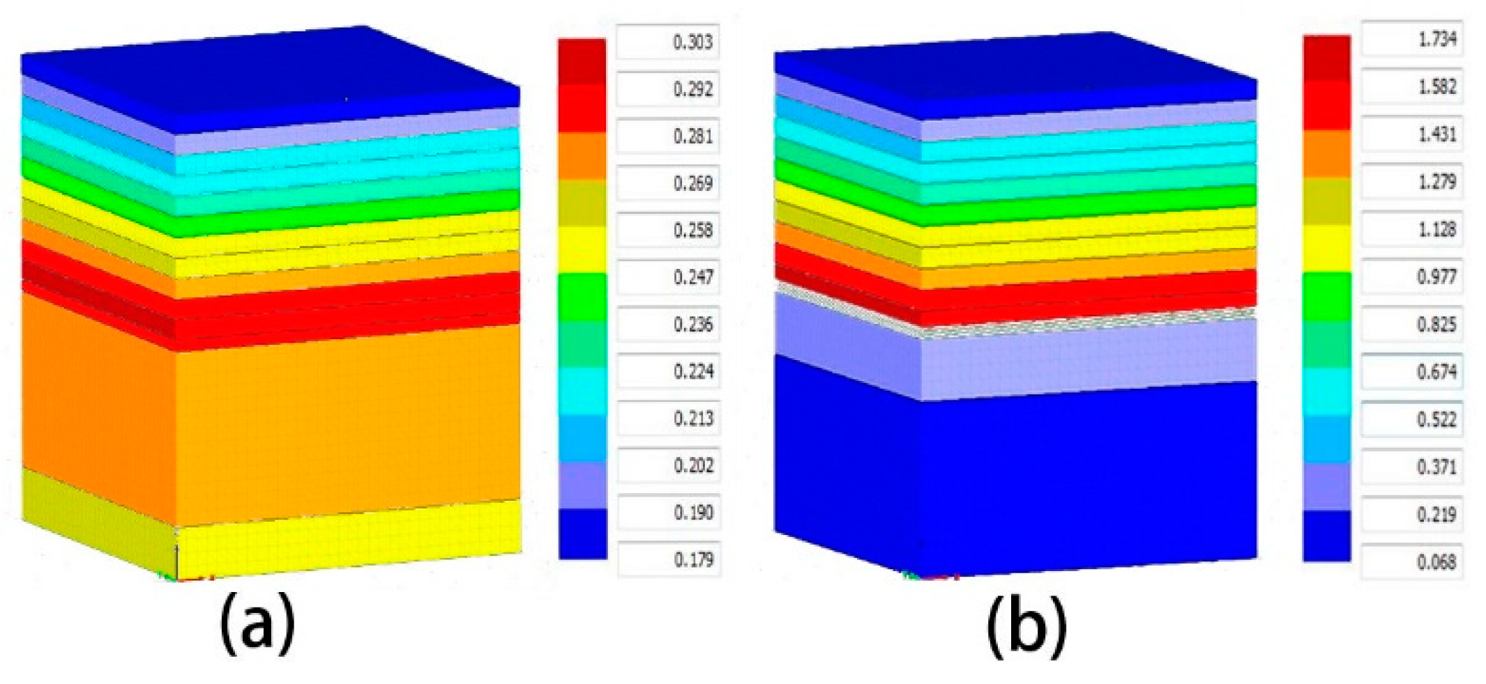
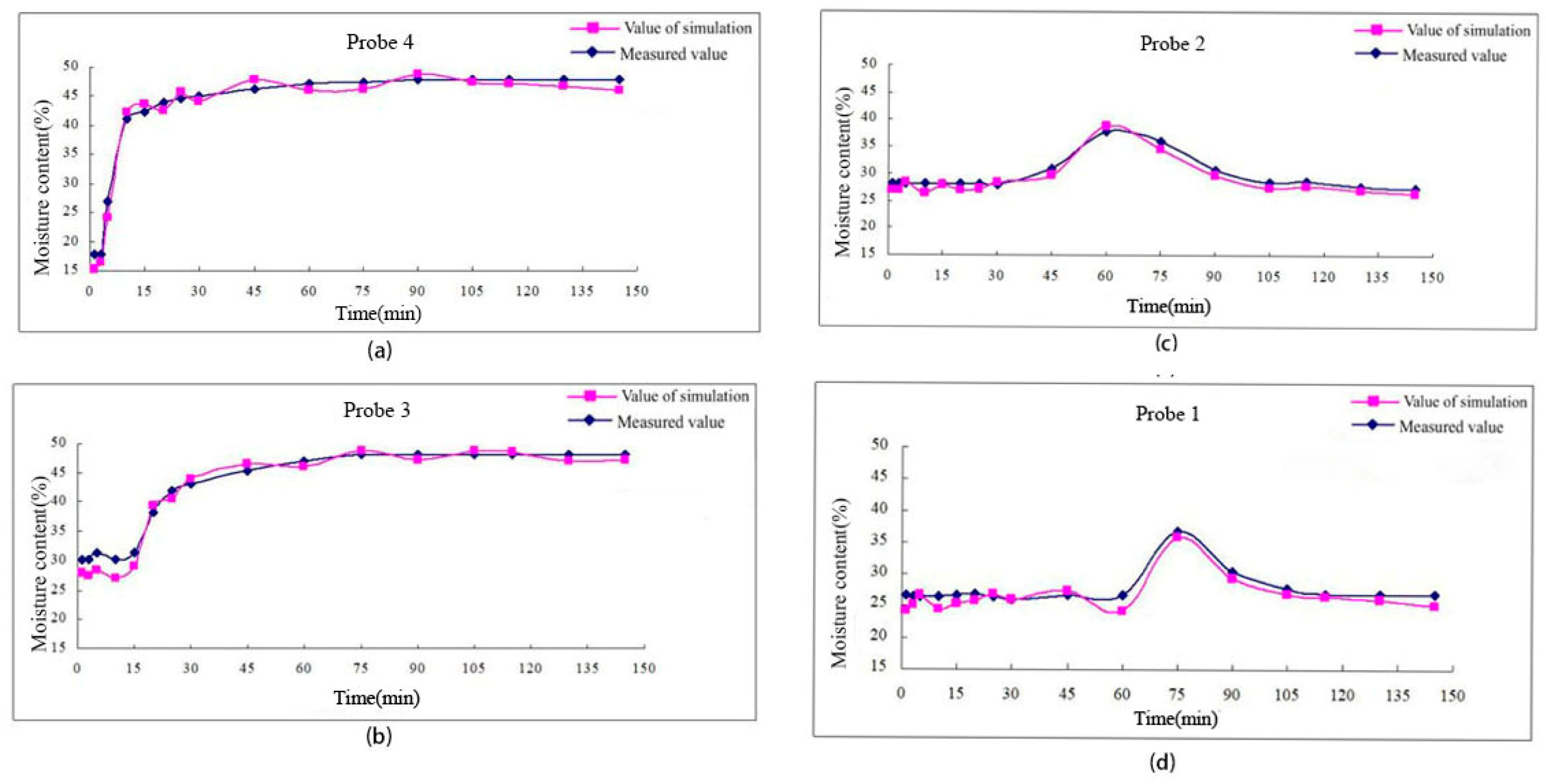
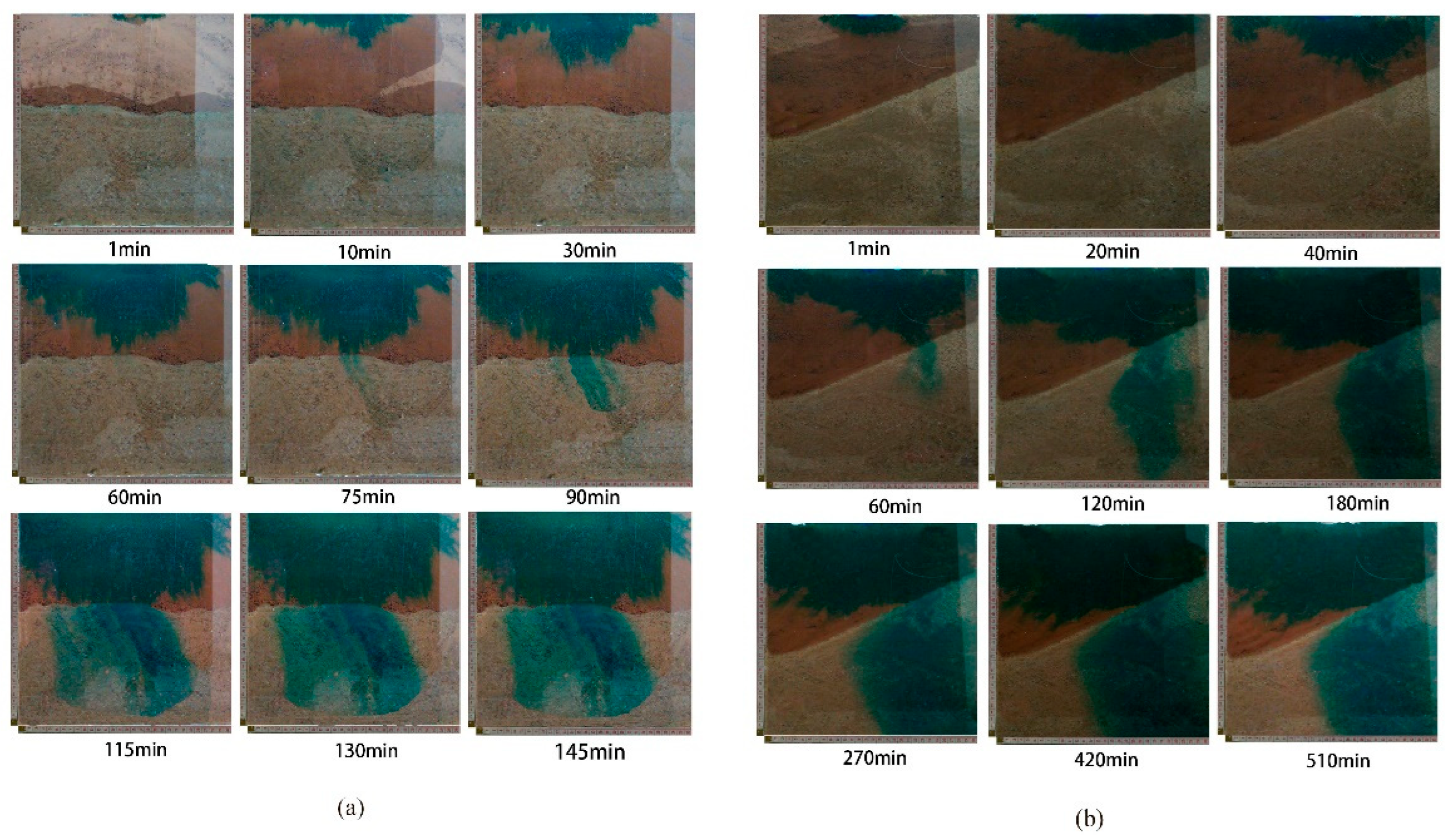
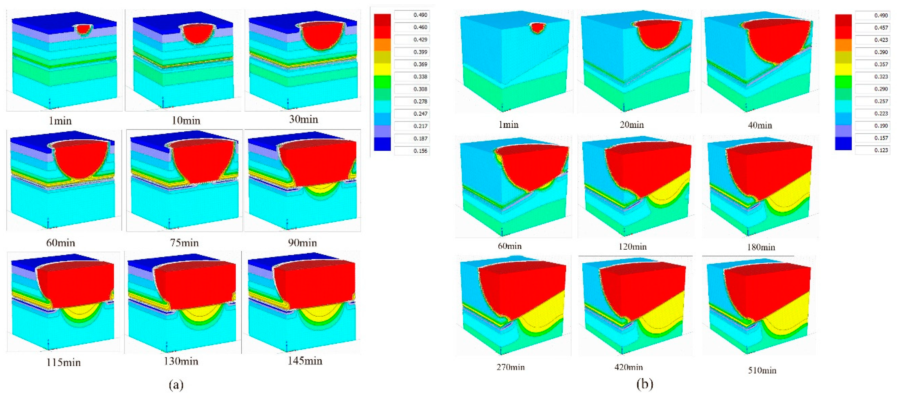
3.1. Characteristics of Water Transport under a Horizontal Interface

The comparison diagram between the measured and simulated water values monitored by each probe in horizontal contact mode is depicted in Figure 3, and it can be seen that the measured and simulated values are similar. Probes 4 and 3 were located in the topsoil, and their moisture changes increased and stabilized over time. Both probe 2 and probe 1 were located in sandy soil, where the moisture change gradually increased, then decreased, and then stabilized [31]. In the first 10 min of adding water, probe 4 in the uppermost layer reached more than 40%. From the simulation effect in Figure 3, it can also be deduced that the initial velocity of water migration was greater, thereby highlighting the characteristics of water change. Probes 3 and 2 were close to the interface of the two layers of soil, and their maximum values were observed around 60 min later. There was about a 15 min time difference between probe 1 and probe 2. The change in probe water in sand only showed an abrupt increase when water had just passed through the sand. When water is completely submerged in sand, the water content of the sand tends to become fixed but is greater than the initial water content [32].

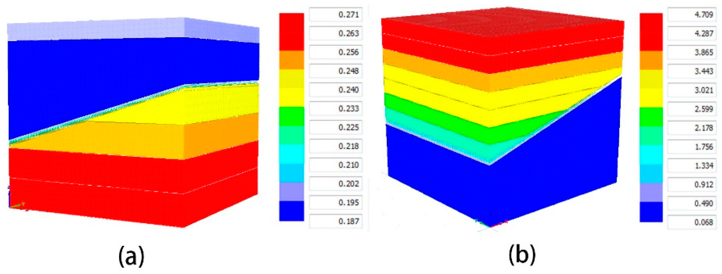
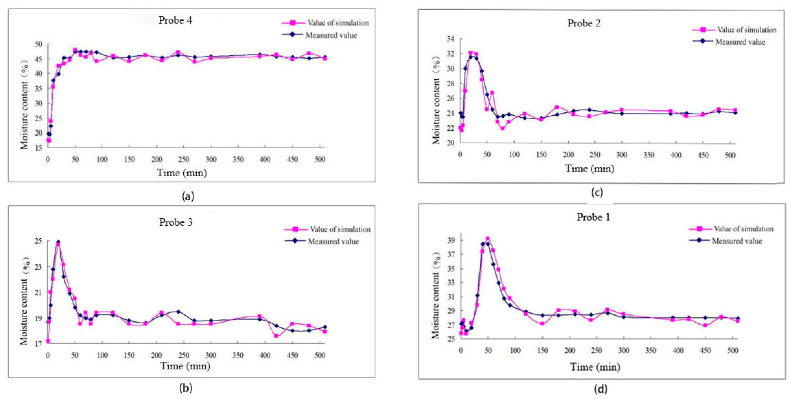
3.2. Characteristics of Water Transport under the Inclined Interface

Figure 4 compares the measured and simulated water values monitored by each probe in the inclined contact mode. Probe 4 was located in the surface soil, whereas probes 3, 2, and 1 were in the sandy soil [33].
As depicted in the figure below, the measured and simulated water contents under the inclined contact mode follow a similar trend, with minor deviations at specific times. Probe 4 in the topsoil reached 45% within 10 min and stabilized at about 45% within 500 min. Probes 3, 2, and 1 in sandy soil showed an increasing and then decreasing trend [34]. However, compared with probes 2 and 1 in sandy soil under horizontal contact mode, these three trends did not remain stable for an extended period of time and showed an initial trend of gradual increase. The peak values of the three probes showed a time lag; the peak values of probes 3 and 2 showed a time lag of 10 min, while those of probes 2 and 1 showed a time lag of 15 min.

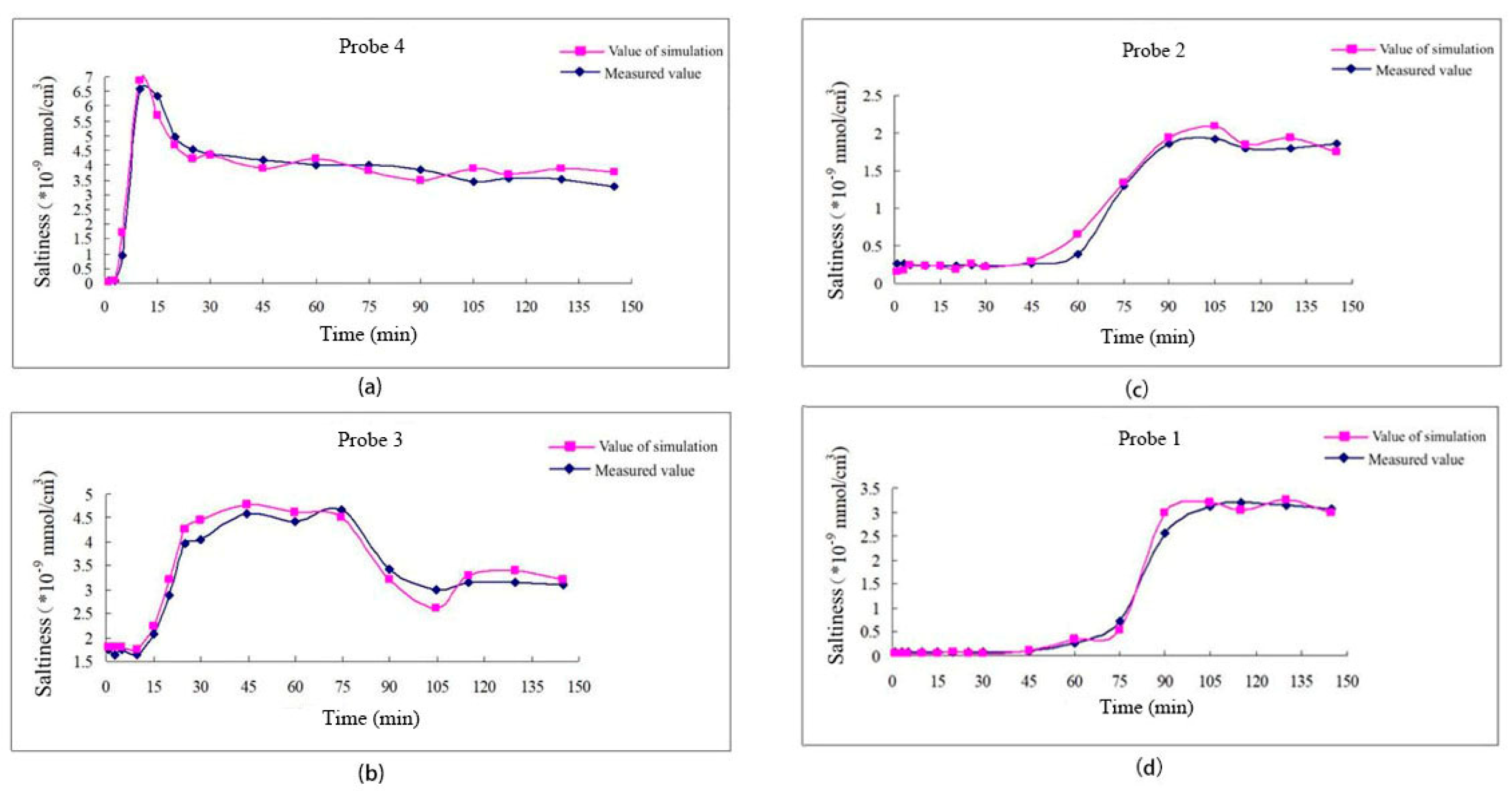
3.3. Characteristics of Salt Migration under a Horizontal Interface

Figure 5 shows a comparison of the measured salt data monitored by each probe in the horizontal contact mode to the simulated values. The salinity of probes 4 and 3 in the surface soil initially increased, then decreased, and then tended to remain stable [35]. However, the salinity changes of probes 2 and 1 in sandy soil gradually increased and stabilized, exhibiting characteristics opposite to those of water.
As shown in Figure 5, probe 4 in the surface soil reached its maximum value around 10 min; then, during the gradual irrigation process, the salt content of the soil decreased until it stabilized at 4 × 10⁻⁹ mmol/cm3 when the irrigation was stopped at 115 min. The maximum value of probe 3 was observed at around 45 min, with a fluctuating range between 45 min and 75 min. It began to decrease after 75 min and remained at 3.3 × 10⁻⁹ mmol/cm3 until the end of the simulation [36,37,38]. The salt content of the surface soil was stable at both the beginning and end of the experiment, but it was higher at the end. With the downward movement of water, the surface soil accumulates salt, which adsorbs on the surface of soil particles, causing the salt content to rise. From the beginning of the simulation to 75 min later, both probe 2 and probe 1 in sandy soil were in a steady and slow-rising stage, with a 15 min time lag between the two. In general, the simulated and measured values of the four probes are quite similar, with minor deviations at certain times [39,40].

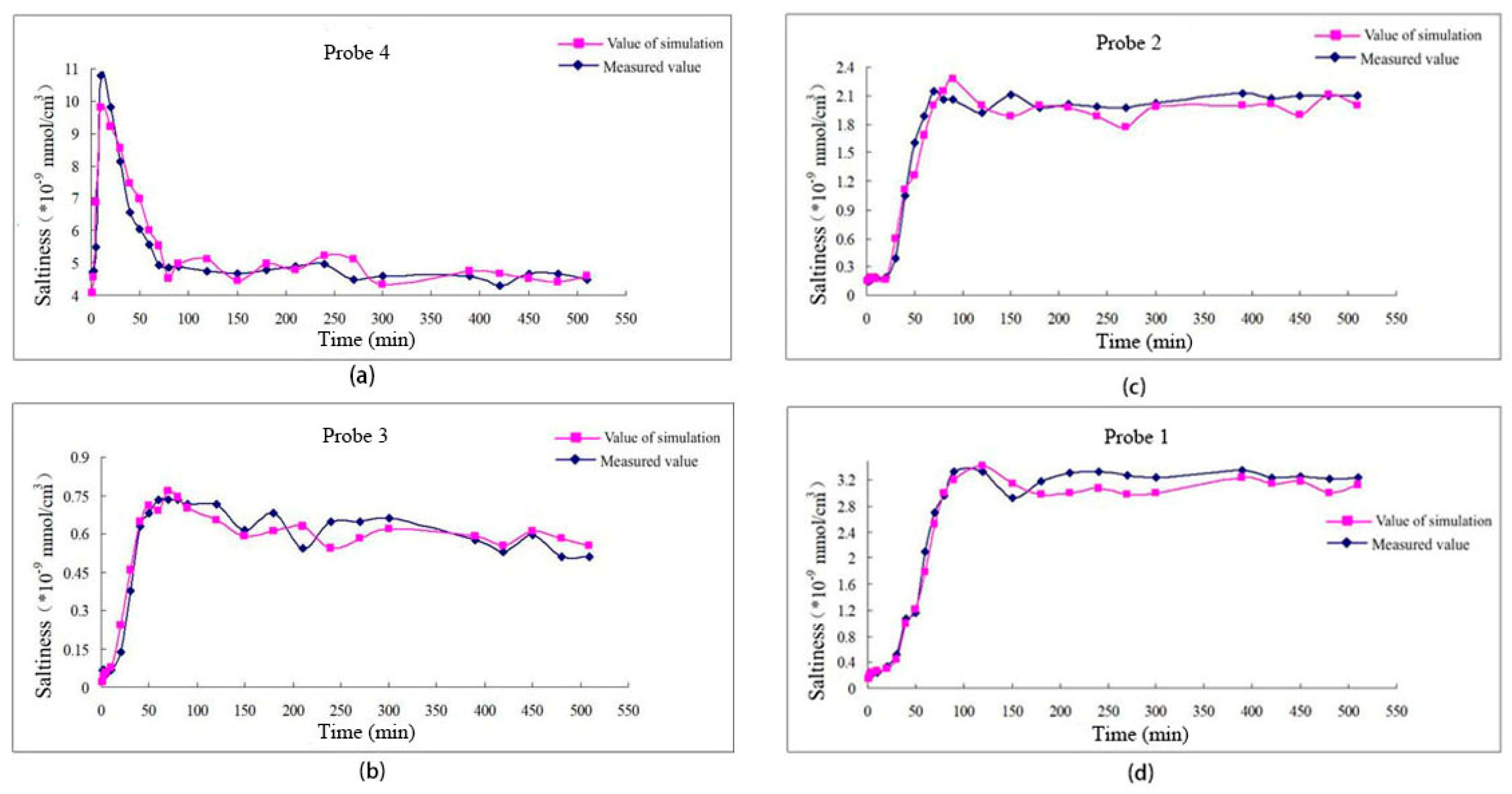
3.4. Characteristics of Salt Transport at an Inclined Interface

Figure 6 depicts a comparison between the measured and simulated values of soil salt under the inclined contact mode. The trend of these values appears to be quite similar. Probe 4 reached its maximum value in about 10 min, with a simulated value of 10 × 10−9 mmol/cm3 and a measured value of about 10.8 × 10⁻⁹ mmol/cm3. By 60 min, the salt content had decreased to about 5 × 10⁻⁹ mmol/cm3 and remained stable for the next 450 min. All three sandy-soil-based probes—3, 2, and 1—showed a slow increase to the maximum value after the region became stable. There was a certain time lag between the three: the maximum value of probe 3 reached about 70 min, probe 2 reached about 90 min, and probe 1 reached about 120 min.

3.5. Model

The model is evaluated using the root-mean-square error (RMSE) and the Nash efficiency coefficient (NSE). When the values of RMSE and E are closer to 0 and 1, respectively, the simulation effect is considered to be optimal. Table 1 reveals that the RMSE value of the water simulation effect of each probe in horizontal contact mode ranges from 0.102 to 0.273, with probe 3 having the greatest simulation difference and probe 2 having the best simulation effect. The E value of probe 4 is between 0.732 and 0.978. Probe 4 has the best simulation effect, and probe 1 has the smallest E value. It seems that the moisture-fitting effect is up to standard and the model is reliable. The RSME value of salt in horizontal contact mode ranges from 0.128 to 0.31, and the effect of probe 1 is the best, while the difference of probe 4 is larger. The E value is between 0.946 and 0.991, and its data are generally close to 1. The simulation effect of the model is more reliable than the effect of moisture [41]. Under inclined contact mode, the RMSE value of the moisture evaluation index ranges from 0.132 to 0.479, with the difference between probe 4 and probe 2 being the most pronounced. The E value is between 0.778 and 0.961, with probe 2 having the lowest value and probe 4 having the highest. The close proximity of the RMSE and E values to 0 and 1, respectively, indicates that the model closely resembles the actual situation [42]. The RMSE values for the salt evaluation index range from 0.052 to 0.548, with probe 3 having the lowest value and probe 4 having the highest. The E value ranges from 0.899 to 0.983, with probe 4 having the smallest value and probe 1 having the largest; however, as the data satisfy the minimum requirements, the numerical simulation model under the inclined contact mode is deemed reliable.

3.6. Discussion of Simulation Results

3.6.1. 3D Simulation

The water and salt migration characteristics of the surface soil and sand soil under two conditions are simulated by the three-dimensional soil column model. The results show that the water in the surface soil reached the irrigation point and the center reached the saturation state, with the surrounding water diffusing in the same circle [43].
The migration process, as captured by the camera in horizontal contact mode, is shown in Figure 7a. The water initially diffused in concentric circles as it was injected into the soil box, resulting in greater soil moisture near the irrigation point. During diffusion, the water content near the central point was higher, and the change in water became more obvious the farther from the outer layer. Due to the small diffusion range in the early stage, the water concentration was mainly about 40% near the irrigation point. At the beginning, the diffusion speed was fast, and the water had spread to 7 cm below the surface in about 25 min. Water changed at the interface of the two soil layers for approximately 60 min as a result of the difference in permeability coefficient between the upper and lower soil layers. At 75 min, water started to diffuse to the left and right through a hole in the interface that the outermost layer of water had created. After 60 min, a discernible change in the moisture content of the lower layer of sand occurred, similar to a secondary pollution phenomenon. The more excessive the water, the interface continued to penetrate downward in the form of concentric circles. Figure 8a shows the simulated process of penetration. Upon secondary infiltration, it was found that the maximum water content at the central point of the sand was 36.9%, while the maximum water content at the central point of the surface soil did not exceed 40%. Additionally, as one goes down, the water content decreases. After about 100 min, the top layer of soil was nearly entirely saturated on the profile, while the lowermost layer of sand remained uncontaminated by irrigation.
Given that the experiment only reveals the migration characteristics of the wetting peak on the section, the numerical simulation provides the means to determine the three-dimensional variation of the wetting peak. Water diffused in concentric circles around the water filling point on the surface above, but the transverse diffusion rate was significantly slower than the longitudinal diffusion rate. The wetting peak made contact with the interface between the two soil layers at the 60 min mark, whereas the horizontal wetting peak only extended to one-half of the surface. The diffusion changes were comparatively smaller on the side, and the linear distribution of water underwent a change only after 75 min. In the subsequent 80 min, a red saturated water phenomenon started to appear on the left and right sides, and irrigation started to cover the water in the surface soil. The moisture characteristics showed an arc distribution along the side, with a larger y-axis that decreased towards the front. The moisture characteristics of the sand side remained relatively constant. Specifically, the moisture penetrated the interface after 60 min, resulting in the accumulation of moisture on the side at the interface. Subsequently, the moisture content in the lower portion remained at a mere 25% until the end of the simulation [44].
In the way the soil is inclined to contact, set the time step to 510 min, and according to the test process, the corresponding time wetting feature diagram (Figure 8b) and the actual migration process recorded by the sensor (Figure 7b) are output. Moisture changes at the onset of irrigation in a manner similar to horizontal contact. Water diffuses in concentric circles near the filling point, where it is nearly saturated. Initially, the diffusion rate was high, reaching 7 cm after 20 min and approaching the interface after 40 min. It was observed that the gradient variation is greater and the variation in water content is more pronounced near the interface. The wetting peak starts to penetrate the interface when the moisture content of the outermost layer matches that of the interface. After 50 min, the moisture content of the sand began to change, and the interface occurred at a particular angle. Initially, the interface wetting peak appeared as concentric circles; however, 120 min later, it was observed that the concentric circles had shifted. Saturated water was nearly entirely present in the upper soil layer, which caused the moisture to come into contact with the interface near the right side of the soil box. The right wetting peak in the sand created a gap, which grew greater and more pronounced as time passed. At the 390 min mark, the water content on the right side of the sand’s center point in the soil box was nearly complete, whereas the left side had undergone arc diffusion.
On the upper surface, the variational characteristics of the wetting peak were observed. The wetting peak on the surface dissipated by half within 50 min due to the transverse diffusion rate being lower than the longitudinal diffusion rate. At the 60 min mark, the upper-right corner of the water gradient in the lateral soil tank began to change; after an additional 60 min, the upper-right corner stabilized as the center began to fan out. Saturated water affects the linear change in the initial water content of the surface soil, whereas the outer layer of the wetting peak has a steeply varying water content gradient. At the end of the experiment, a quarter-oval had formed in the side surface soil. At 50 min, when the wetting peak diffused to the interface, the lateral water content of the underlying sand shifted to a predominantly linear distribution. Water continues to accumulate in close proximity to the interface, and the rate of water loss in the sand is excessively rapid, preventing it from reaching saturation like the surface soil [45].
A soil column model was constructed using the HYDRUS-3D software (HYDRUS 2.05) to simulate both inclined and horizontal contact modes. This model was used to assess the reliability of the experiment and analyze the transport characteristics of water, salt, and moisture peaks under various contact conditions [40,46].
After comparing and analyzing the observed data with the simulated data, it was determined that the trends of simulated and measured salt and water values are nearly identical, with only minor fluctuations at various times. In contrast to the sand soil, which showed a pattern like a normal curve, the water content of the surface soil increased gradually before stabilizing. The salt characteristics exhibited by the surface soil followed a normal distribution curve, whereas those of the sandy soil increased gradually before reaching a state of stability [47,48]. The findings of this study correlate with the results obtained by Wang et al. [13].

3.6.2. Water Salt Simulation

Comparing and analyzing the simulated and observed data revealed some similarity between the experimental and simulated data for salt and water [49,50]. Moisture in the sand follows a pattern like a normal curve, whereas moisture in the surface soil increases gradually until it reaches a stable trend. The salt characteristics of the surface soil show a trend that resembles a normal curve, whereas those of the sand increase gradually to a steady degree [51].

4. Conclusions

In this study, the effects of different soil contact modes on water and salt movement in soil were studied through laboratory experiments and numerical simulations with the following objectives:
(i)
Objective 1: Laboratory experiments were conducted to investigate the laws of water and salt transport under different soil interface contact modes. The results show that surface soil and sandy soil transport water differently. Additionally, the transport laws for salt vary between the two soil types. The salt content of the surface soil exhibits a rapid increase and a subsequent decrease; this is in contrast to the sandy soil, which increases gradually to its maximum value before stabilizing. The monitoring data from the probe’s two contact modes reveal a certain lag in water and salt transport in the soil.
(ii)
Objective 2: To explore the fitting degree of the Hydrus-3D model to simulate the contact relationship between different soil interfaces. The HYDRUS software was used to develop two types of groundwater salt transport models, namely, horizontal contact and inclined contact, and the simulation results were validated by indoor monitoring data. The results show that the model accurately replicates the water and salt transport rules under the two contact modes and that the time variation rules of water and salt contents simulated by the model are comparable to the indoor monitoring data. Understanding the law of water and salt migration is the key to improving and preventing soil salinization. It is helpful to understand the law of water and salt migration in soil and groundwater. As a result of the experimental approach, this paper replicates the migration process using only a soil box for the indoor experiment. Future studies may benefit from the integration of laboratory experiments and field-scale measurements, as well as the application of the Hydrus-3D model as a simulation technique to further investigate the model’s feasibility in light of the dearth of field-scale monitoring data.
The results of this study are useful for understanding the dynamic change characteristics of different soils with water and salt infiltration contact, and for developing engineering or non-engineering methods to improve the environmental conditions of underground soil, which has important theoretical and practical significance.

Author Contributions

Conceptualization, X.L. and Y.H.; methodology, Y.H. and Z.Y.; software, Y.H., L.W. and M.S.; validation, X.L., Z.Y. and L.W.; formal analysis, Y.H. and Z.Y.; investigation, X.L., M.S. and L.W.; resources, X.L. and M.S.; data curation, X.L. and Y.H.; writing—original draft preparation, Y.H., Z.Y., A.R. and M.S.; writing—review and editing, L.W., M.S. and A.R.; visualization, X.L. and Y.H.; supervision, Y.H.; project administration, X.L.; funding acquisition, X.L. All authors have read and agreed to the published version of the manuscript.

Funding

This study was financed by the National Natural Science Foundation of China (Grant No. 51979078) and Jiangsu Provincial Geological Exploration Fund Project “Yangtze River Delta Eco-Green Integrated Development Demonstration Zone (Jiangsu) Eco-Geological Survey”.

Data Availability Statement

The data already exist in the manuscript.

Conflicts of Interest

The authors declare no conflict of interest.

References

  1. Gupta, B.; Huang, B. Mechanism of salinity tolerance in plants: Physiological, biochemical, and molecular characterization. Int. J. Genom. 2014, 2014, 701596. [Google Scholar] [CrossRef]
  2. Yang, T.; Hu, L.; Petrů, M.; Wang, X.; Xiong, X.; Yu, D.; Mishra, R.; Militký, J. Determination of the permeability coefficient and airflow resistivity of nonwoven materials. Text. Res. J. 2021, 92, 126–142. [Google Scholar] [CrossRef]
  3. Ebrahimi, A.; Kleijn, C.R.; Richardson, I.M. Sensitivity of Numerical Predictions to the Permeability Coefficient in Simulations of Melting and Solidification Using the Enthalpy-Porosity Method. Energies 2019, 12, 4360. [Google Scholar] [CrossRef]
  4. Issa, R. Solution of the implicitly discretised fluid flow equations by operator-splitting. J. Comput. Phys. 1986, 62, 40–65. [Google Scholar] [CrossRef]
  5. Sun, D.; Yang, H.; Guan, D.; Yang, M.; Wu, J.; Yuan, F.; Jin, C.; Wang, A.; Zhang, Y. The effects of land use change on soil infiltration capacity in China: A meta-analysis. Sci. Total Environ. 2018, 626, 1394–1401. [Google Scholar] [CrossRef] [PubMed]
  6. Liu, Y.; Cui, Z.; Huang, Z.; López-Vicente, M.; Wu, G.-L. Influence of soil moisture and plant roots on the soil infiltration capacity at different stages in arid grasslands of China. Catena 2019, 182, 104147. [Google Scholar] [CrossRef]
  7. Wu, G.-L.; Yang, Z.; Cui, Z.; Liu, Y.; Fang, N.-F.; Shi, Z.-H. Mixed artificial grasslands with more roots improved mine soil infiltration capacity. J. Hydrol. 2016, 535, 54–60. [Google Scholar] [CrossRef]
  8. Murakami, M.; Sato, N.; Anegawa, A.; Nakada, N.; Harada, A.; Komatsu, T.; Takada, H.; Tanaka, H.; Ono, Y.; Furumai, H. Multiple evaluations of the removal of pollutants in road runoff by soil infiltration. Water Res. 2008, 42, 2745–2755. [Google Scholar] [CrossRef]
  9. Colman, E.A.; Bodman, G.B. Moisture and Energy Conditions during Downward Entry of Water into Moist and Layered Soils. Soil Sci. Soc. Am. J. 1945, 9, 3–11. [Google Scholar] [CrossRef]
  10. Hanks, R.J.; Bowers, S.A. Numerical Solution of the Moisture Flow Equation for Infiltration into Layered Soils. Soil Sci. Soc. Am. J. 1962, 26, 530–534. [Google Scholar] [CrossRef]
  11. Hillel, D.; Baker, R.S. A descriptive theory of fingering during infiltration into layered soils. Soil Sci. 1988, 146, 51–56. [Google Scholar] [CrossRef]
  12. Toride, N.; Leij, F.J. Convective-Dispersive Stream Tube Model for Field-Scale Solute Transport: I. Moment Analysis. Soil Sci. Soc. Am. J. 1996, 60, 342–351. [Google Scholar] [CrossRef]
  13. Wang, D.; Fei, L. Rise in layered soil capillary water moves the characteristic test research. J. Groundw. 2009, 31, 4. [Google Scholar] [CrossRef]
  14. Li, Y.; Ren, X.; Horton, R. Effects of different textures and interlayer locations on infiltration rules of layered soil. J. Drain. Irrig. Mach. Eng. 2012, 30, 6. [Google Scholar] [CrossRef]
  15. Selker, J.; Stewart, R. Soil Physics with HYDRUS: Modeling and Applications. Vadose Zone J. 2011, 10, 1338–1339. [Google Scholar] [CrossRef]
  16. Dou, X.; Shi, H.; Li, R.; Miao, Q.; Yan, J.; Tian, F.; Wang, B. Simulation and evaluation of soil water and salt transport under controlled subsurface drainage using HYDRUS-2D model. Agric. Water Manag. 2022, 273, 107899. [Google Scholar] [CrossRef]
  17. Asgari, M.; de Zélicourt, D.; Kurtcuoglu, V. Glymphatic solute transport does not require bulk flow. Sci. Rep. 2016, 6, 38635. [Google Scholar] [CrossRef]
  18. Zhang, C.; Jia, L.; Shen, Y.; Ma, C. The Influence of Straw Mulch on the Transport and Distribution of Water and Salt in Indirect Drip Irrigation with Saline Water. In Sustainable Development of Water Conservancy Projects in China; Springer, 2019; pp. 227–239. [Google Scholar] [CrossRef]
  19. Sahin, U.; Ekinci, M.; Ors, S.; Turan, M.; Yildiz, S.; Yildirim, E. Effects of individual and combined effects of salinity and drought on physiological, nutritional and biochemical properties of cabbage (Brassica oleracea var. capitata). Sci. Hortic. 2018, 240, 196–204. [Google Scholar] [CrossRef]
  20. Miah, M.Y. Impact of salinity intrusion on agriculture of Southwest Bangladesh—A review. Int. J. Agric. Policy Res. 2020, 8, 40–47. [Google Scholar] [CrossRef]
  21. Liu, X.; Lu, X.; Zhao, W.; Yang, S.; Wang, J.; Xia, H.; Wei, X.; Zhang, J.; Chen, L.; Chen, Q. The rhizosphere effect of native legume Albizzia julibrissin on coastal saline soil nutrient availability, microbial modulation, and aggregate formation. Sci. Total Environ. 2021, 806, 150705. [Google Scholar] [CrossRef]
  22. Lu, J.; Wu, J.; Wu, J.; He, X. Adsorption of nonylphenol on coastal saline soil: Will microplastics play a great role? Chemosphere 2023, 311, 137032. [Google Scholar] [CrossRef] [PubMed]
  23. Moghbel, F.; Mosaedi, A.; Aguilar, J.; Ghahraman, B.; Ansari, H.; Gonçalves, M.C. Uncertainty Analysis of HYDRUS-1D Model to Simulate Soil Salinity Dynamics under Saline Irrigation Water Conditions Using Markov Chain Monte Carlo Algorithm. Agronomy 2022, 12, 2793. [Google Scholar] [CrossRef]
  24. Zhang, Q.; Shen, X. Progress of Water and Salt Transport in Saline Lands and Hydrus Model: A Review. Acad. J. Sci. Technol. 2023, 6, 33–39. [Google Scholar] [CrossRef]
  25. Jia, Y.; Gao, W.; Sun, X.; Feng, Y. Simulation of Soil Water and Salt Balance in Three Water-Saving Irrigation Technologies with HYDRUS-2D. Agronomy 2023, 13, 164. [Google Scholar] [CrossRef]
  26. Sehn, P. Fluoride removal with extra low energy reverse osmosis membranes: Three years of large scale field experience in Finland. Desalination 2008, 223, 73–84. [Google Scholar] [CrossRef]
  27. Zhang, Y.; Ghyselbrecht, K.; Meesschaert, B.; Pinoy, L.; Van der Bruggen, B. Electrodialysis on RO concentrate to improve water recovery in wastewater reclamation. J. Membr. Sci. 2011, 378, 101–110. [Google Scholar] [CrossRef]
  28. Šimůnek, J.; van Genuchten, M.T.; Šejna, M. Development and Applications of the HYDRUS and STANMOD Software Packages and Related Codes. Vadose Zone J. 2008, 7, 587–600. [Google Scholar] [CrossRef]
  29. Robinson, C.; Xin, P.; Li, L.; Barry, D.A. Groundwater flow and salt transport in a subterranean estuary driven by intensified wave conditions. Water Resour. Res. 2013, 50, 165–181. [Google Scholar] [CrossRef]
  30. Oster, J.; Letey, J.; Vaughan, P.; Wu, L.; Qadir, M. Comparison of transient state models that include salinity and matric stress effects on plant yield. Agric. Water Manag. 2012, 103, 167–175. [Google Scholar] [CrossRef]
  31. Sen, T.K.; Khilar, K.C. Review on subsurface colloids and colloid-associated contaminant transport in saturated porous media. Adv. Colloid Interface Sci. 2006, 119, 71–96. [Google Scholar] [CrossRef]
  32. McNeal, J.M.; Balistrieri, L.S. Geochemistry and occurrence of selenium: An overview. In Selenium in Agriculture and the Environment; Wiley, 2015; pp. 1–13. [Google Scholar] [CrossRef]
  33. Liu, Y.; Miao, H.; Chang, X.; Wu, G. Higher species diversity improves soil water infiltration capacity by increasing soil organic matter content in semiarid grasslands. Land Degrad. Dev. 2019, 30, 1599–1606. [Google Scholar] [CrossRef]
  34. Michael, H.A.; Scott, K.C.; Koneshloo, M.; Yu, X.; Khan, M.R.; Li, K. Geologic influence on groundwater salinity drives large seawater circulation through the continental shelf. Geophys. Res. Lett. 2016, 43. [Google Scholar] [CrossRef]
  35. Giménez-Forcada, E. Space/time development of seawater intrusion: A study case in Vinaroz coastal plain (Eastern Spain) using HFE-Diagram, and spatial distribution of hydrochemical facies. J. Hydrol. 2014, 517, 617–627. [Google Scholar] [CrossRef]
  36. Shams, M.; Alam, I.; Chowdhury, I. Aggregation and stability of nanoscale plastics in aquatic environment. Water Res. 2019, 171, 115401. [Google Scholar] [CrossRef]
  37. Baker, R.S.; Hillel, D. Laboratory Tests of a Theory of Fingering during Infiltration into Layered Soils. Soil Sci. Soc. Am. J. 1990, 54, 20–30. [Google Scholar] [CrossRef]
  38. Tang, L.; Iddya, A.; Zhu, X.; Dudchenko, A.V.; Duan, W.; Turchi, C.; Vanneste, J.; Cath, T.Y.; Jassby, D. Enhanced Flux and Electrochemical Cleaning of Silicate Scaling on Carbon Nanotube-Coated Membrane Distillation Membranes Treating Geothermal Brines. ACS Appl. Mater. Interfaces 2017, 9, 38594–38605. [Google Scholar] [CrossRef] [PubMed]
  39. Meriano, M.; Eyles, N.; Howard, K.W. Hydrogeological impacts of road salt from Canada’s busiest highway on a Lake Ontario watershed (Frenchman’s Bay) and lagoon, City of Pickering. J. Contam. Hydrol. 2009, 107, 66–81. [Google Scholar] [CrossRef]
  40. Kim, Y.X.; Kim, Y.X.; Ranathunge, K.; Ranathunge, K.; Lee, S.; Lee, S.; Lee, Y.; Lee, Y.; Lee, D.; Lee, D.; et al. Composite Transport Model and Water and Solute Transport across Plant Roots: An Update. Front. Plant Sci. 2018, 9, 193. [Google Scholar] [CrossRef]
  41. Rahman, M.M.; Hagare, D.; Maheshwari, B.; Dillon, P. Impacts of Prolonged Drought on Salt Accumulation in the Root Zone Due to Recycled Water Irrigation. Water Air Soil Pollut. 2015, 226, 90. [Google Scholar] [CrossRef]
  42. González-Pinzón, R.; Haggerty, R.; Dentz, M. Scaling and predicting solute transport processes in streams. Water Resour. Res. 2013, 49, 4071–4088. [Google Scholar] [CrossRef]
  43. Ramos, T.; Šimůnek, J.; Gonçalves, M.; Martins, J.; Prazeres, A.; Castanheira, N.; Pereira, L. Field evaluation of a multicomponent solute transport model in soils irrigated with saline waters. J. Hydrol. 2011, 407, 129–144. [Google Scholar] [CrossRef]
  44. Twarakavi, N.K.C.; Šimůnek, J.; Seo, S. Evaluating Interactions between Groundwater and Vadose Zone Using the HYDRUS-Based Flow Package for MODFLOW. Vadose Zone J. 2008, 7, 757–768. [Google Scholar] [CrossRef]
  45. He, K.; Yang, Y.; Yang, Y.; Chen, S.; Hu, Q.; Liu, X.; Gao, F. HYDRUS Simulation of Sustainable Brackish Water Irrigation in a Winter Wheat-Summer Maize Rotation System in the North China Plain. Water 2017, 9, 536. [Google Scholar] [CrossRef]
  46. Ramos, T.B.; Darouich, H.; Šimůnek, J.; Gonçalves, M.C.; Martins, J.C. Soil salinization in very high-density olive orchards grown in southern Portugal: Current risks and possible trends. Agric. Water Manag. 2019, 217, 265–281. [Google Scholar] [CrossRef]
  47. Li, H.; Yi, J.; Zhang, J.; Zhao, Y.; Si, B.; Hill, R.L.; Cui, L.; Liu, X. Modeling of Soil Water and Salt Dynamics and Its Effects on Root Water Uptake in Heihe Arid Wetland, Gansu, China. Water 2015, 7, 2382–2401. [Google Scholar] [CrossRef]
  48. Gonçalves, M.C.; Šimůnek, J.; Ramos, T.B.; Martins, J.C.; Neves, M.J.; Pires, F.P. Multicomponent solute transport in soil lysimeters irrigated with waters of different quality. Water Resour. Res. 2006, 42. [Google Scholar] [CrossRef]
  49. Roberts, T.; Lazarovitch, N.; Warrick, A.W.; Thompson, T.L. Modeling Salt Accumulation with Subsurface Drip Irrigation Using HYDRUS-2D. Soil Sci. Soc. Am. J. 2009, 73, 233–240. [Google Scholar] [CrossRef]
  50. Phogat, V.; Mahadevan, M.; Skewes, M.; Cox, J.W. Modelling soil water and salt dynamics under pulsed and continuous surface drip irrigation of almond and implications of system design. Irrig. Sci. 2011, 30, 315–333. [Google Scholar] [CrossRef]
  51. Phogat, V.; Skewes, M.; Cox, J.; Sanderson, G.; Alam, J.; Šimůnek, J. Seasonal simulation of water, salinity and nitrate dynamics under drip irrigated mandarin (Citrus reticulata) and assessing management options for drainage and nitrate leaching. J. Hydrol. 2014, 513, 504–516. [Google Scholar] [CrossRef]
Figure 1. (a) Initial moisture content distribution in horizontal contact mode. (b) Initial salt distribution map under horizontal contact mode.
Water 16 00047 g001
Figure 2. (a) Initial moisture content distribution in inclined contact mode. (b) Initial salt distribution map under inclined contact mode.
Water 16 00047 g002
Figure 3. Comparison of simulated and measured water content in horizontal contact mode. (a) Probe 4, (b) Probe 3, (c) Probe 2, and (d) Probe 1.
Water 16 00047 g003
Figure 4. Comparison of simulated and measured water content in inclined contact mode. (a) Probe 4, (b) Probe 3, (c) Probe 2, and (d) Probe 1.
Water 16 00047 g004
Figure 5. Comparison of simulated and measured salt content in horizontal contact mode. (a) Probe 4, (b) Probe 3, (c) Probe 2, and (d) Probe 1.
Water 16 00047 g005
Figure 6. Comparison of simulated and measured salt content in inclined contact mode. (a) Probe 4, (b) Probe 3, (c) Probe 2, and (d) Probe 1.
Water 16 00047 g006
Figure 7. (a) Wet peak transport diagram in horizontal contact mode. (b) Wet peak transport diagram in inclined contact mode.
Water 16 00047 g007
Figure 8. (a) Simulation diagram of wet peak migration in horizontal contact mode. (b) Simulation diagram of wet peak migration in inclined contact mode.
Water 16 00047 g008
Table 1. Model reliability analysis.
Soil Contact ModeEvaluation IndexEffect of Water Simulation EvaluationSalt Simulation Evaluation Effect
Probe 1Probe 2Probe 3Probe 4Probe 1Probe 2Probe 3Probe 4
Horizontal contactRMSE0.1330.1020.2730.1510.1280.1950.2290.310
E0.7320.8810.9470.9780.9910.9810.9500.946
Inclined
contact
RMSE0.2180.1320.3670.4790.1640.1390.0520.548
E0.9100.7780.8690.9610.9830.9680.9530.899
Disclaimer/Publisher’s Note: The statements, opinions and data contained in all publications are solely those of the individual author(s) and contributor(s) and not of MDPI and/or the editor(s). MDPI and/or the editor(s) disclaim responsibility for any injury to people or property resulting from any ideas, methods, instructions or products referred to in the content.

