
Improvement in Operation Efficiency of Shallow Geothermal Energy System—A Case Study in Shandong Province, China

Abstract
:1. Introduction
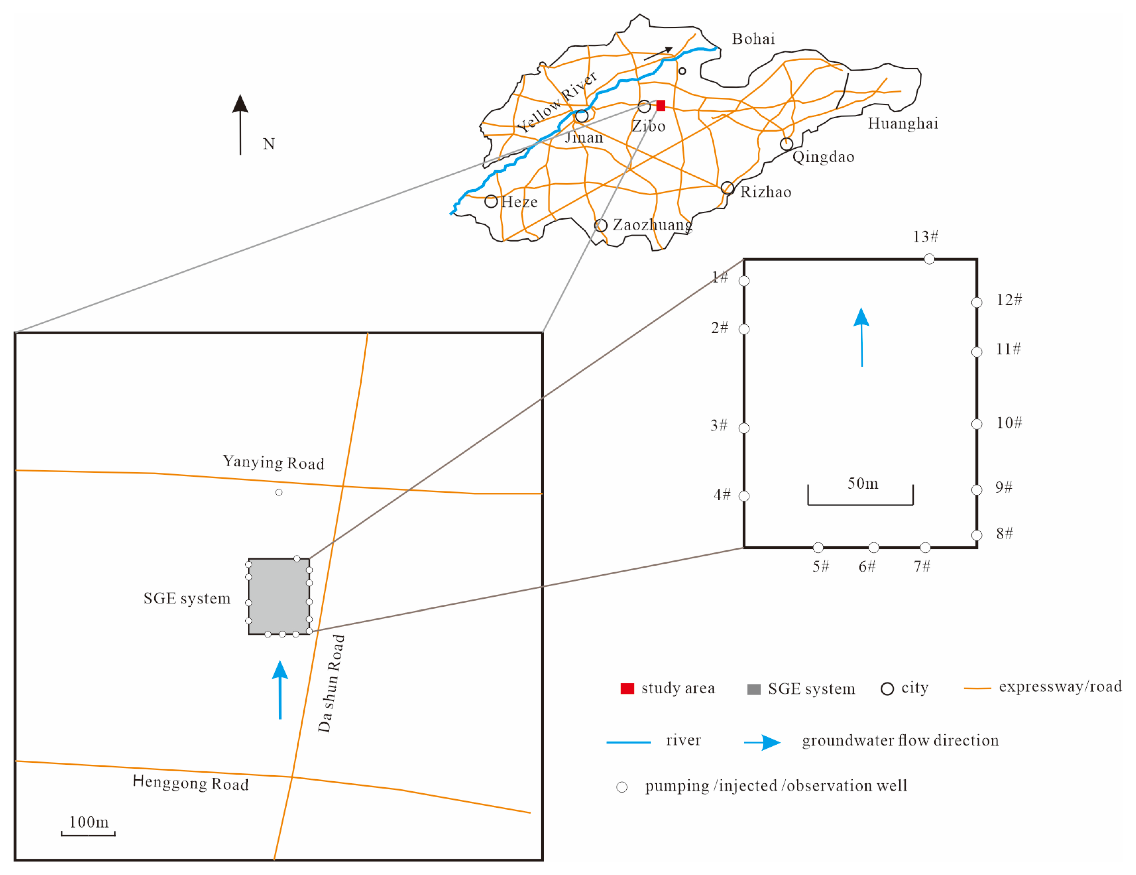
2. Study Area
2.1. Meteorology and Hydrology
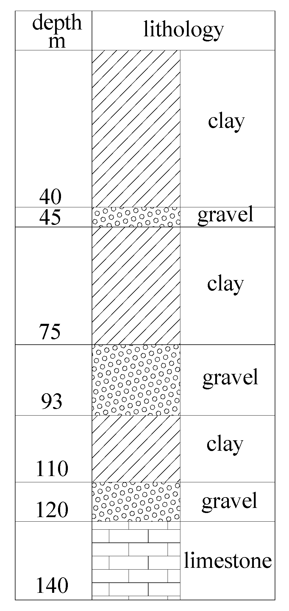
2.2. Hydrogeology
2.3. Operation of the Shallow Geothermal Energy System
3. Methods
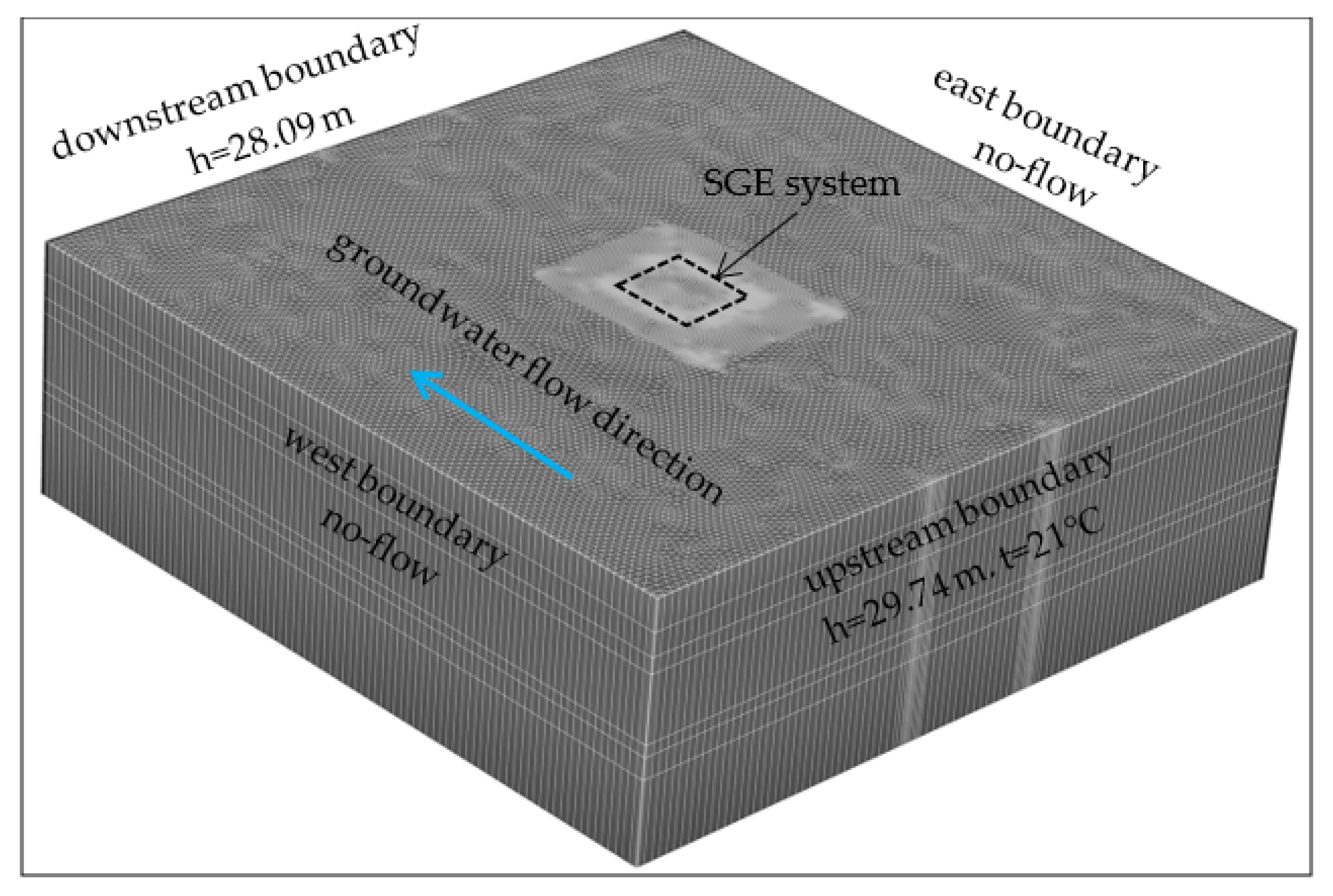
3.1. Conceptual Model of Hydrogeology
3.2. Mathematical Model
3.2.1. Mathematical Model of Groundwater Flow
3.2.2. Mathematical Model of Thermal Transport
3.2.3. Model Condition Setting
- (1)
- Boundary condition
- (2)
- Initial conditions
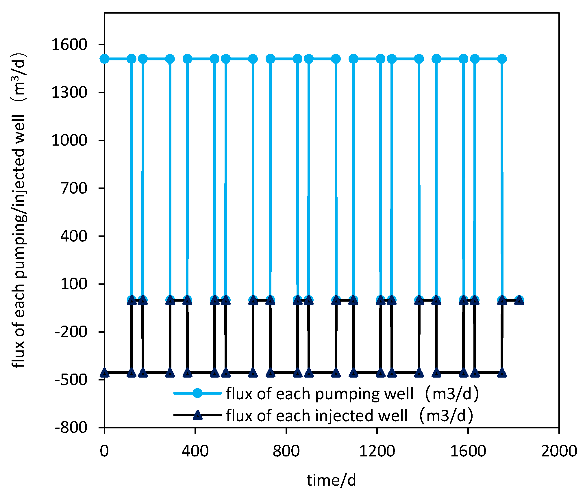
3.3. Simulation Scheme
4. Results
4.1. Simulation of the Current Operation Scheme
4.1.1. Characteristics of Groundwater Flow
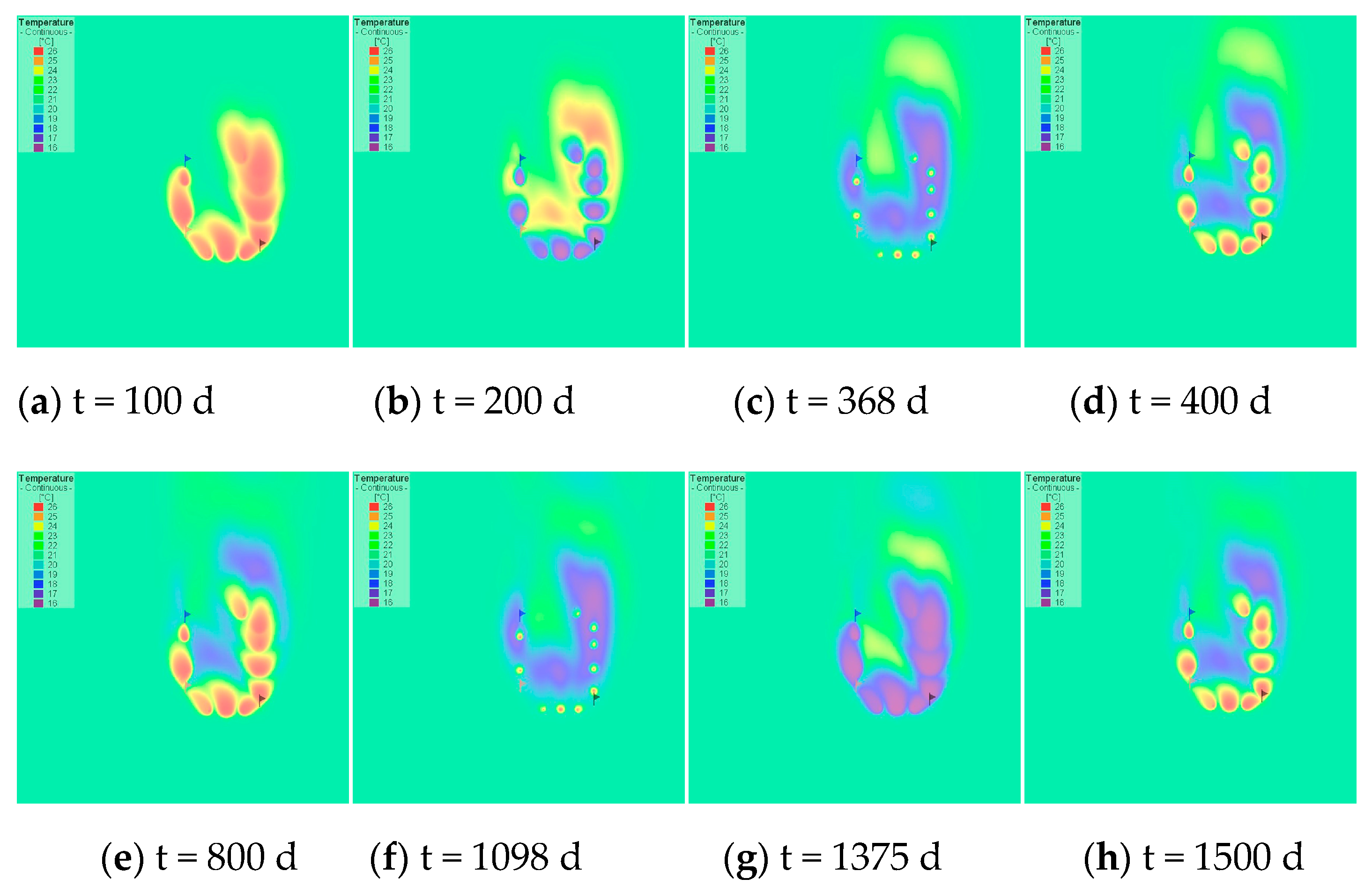
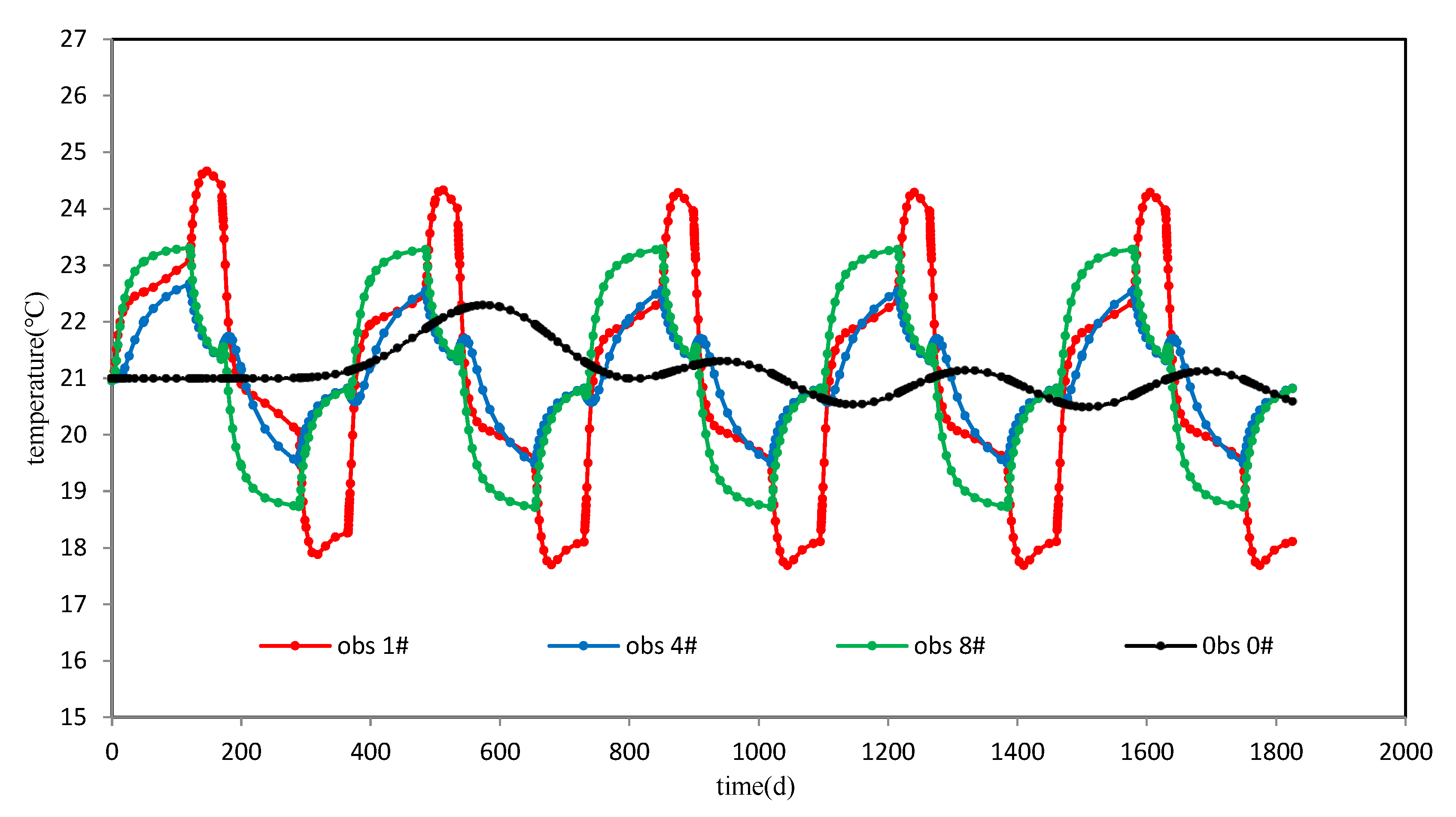
4.1.2. Characteristics of Thermal Transport
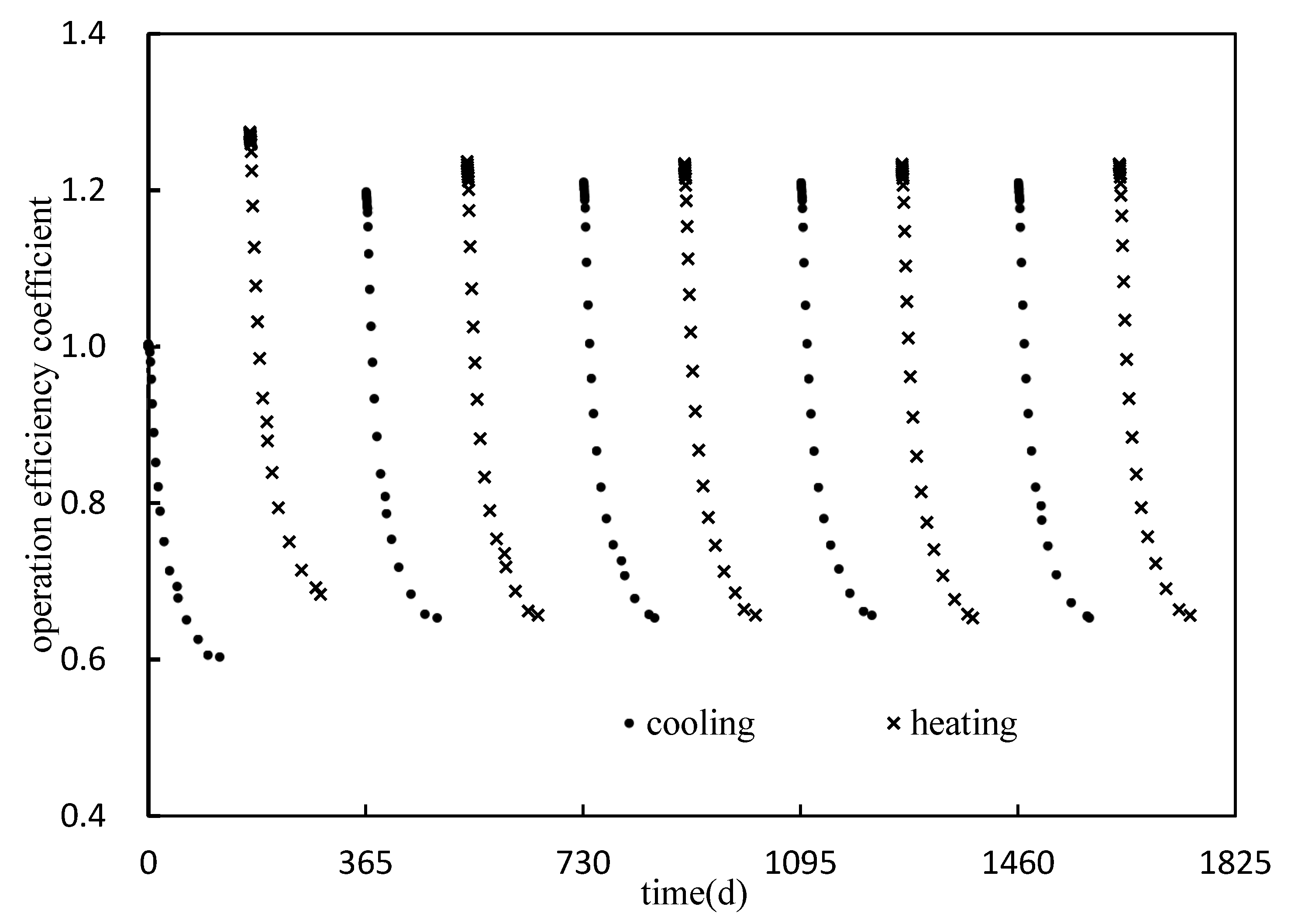
4.1.3. Operation Efficiency Evaluation of the SGE System
4.2. Simulation of the Optimized Operation Schemes
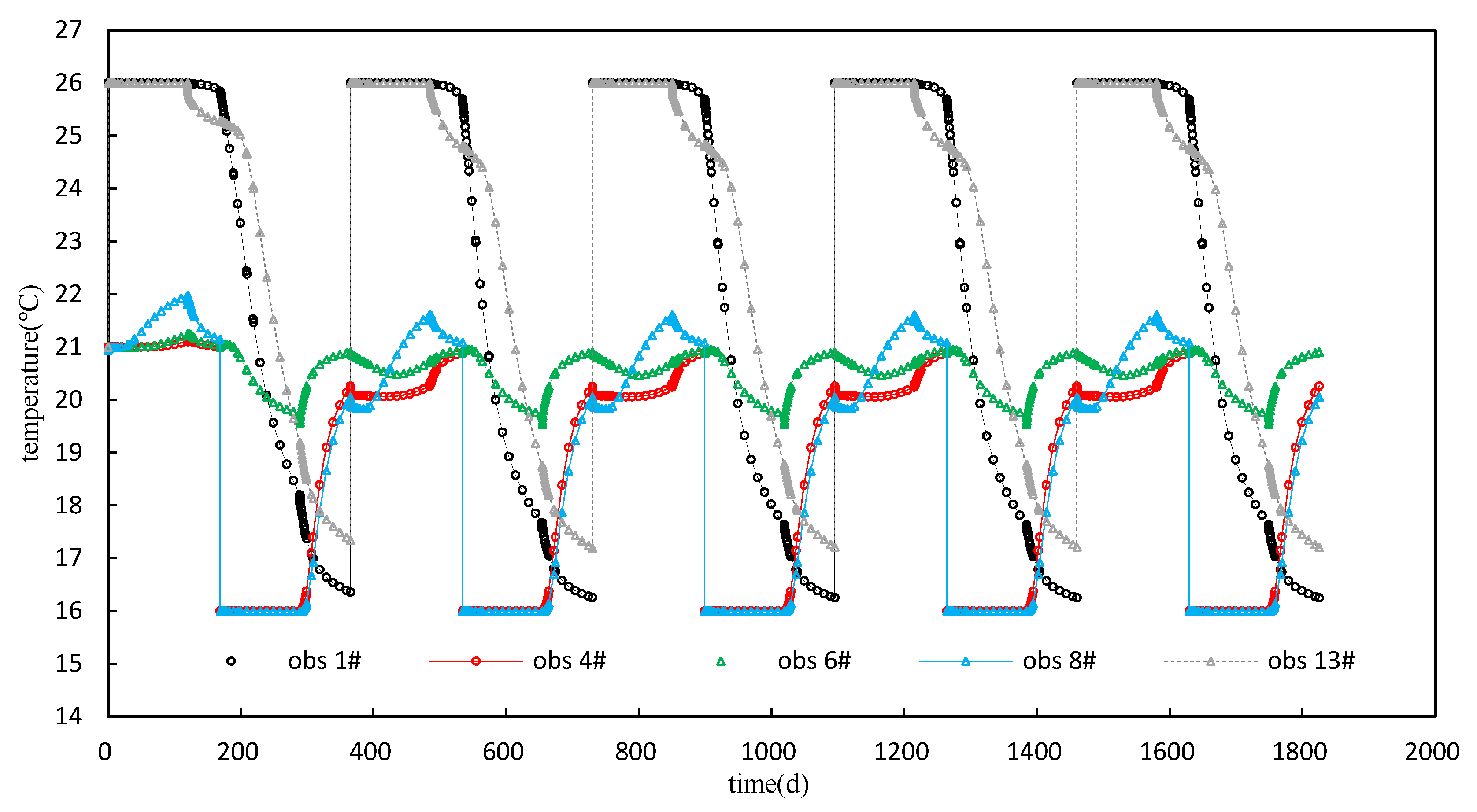
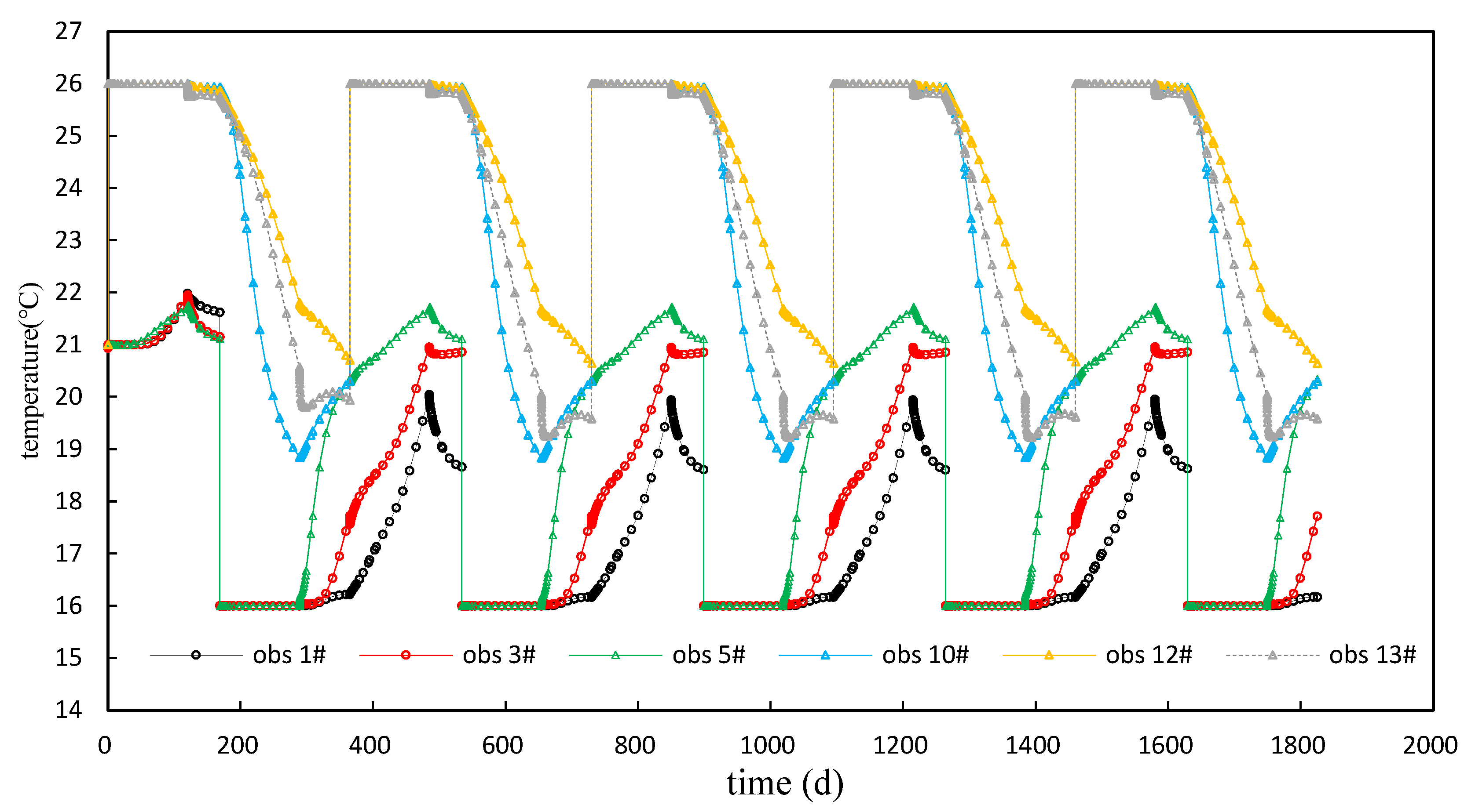
4.2.1. Characteristics of Thermal Transport for F2
4.2.2. Characteristics of Thermal Transport for F3
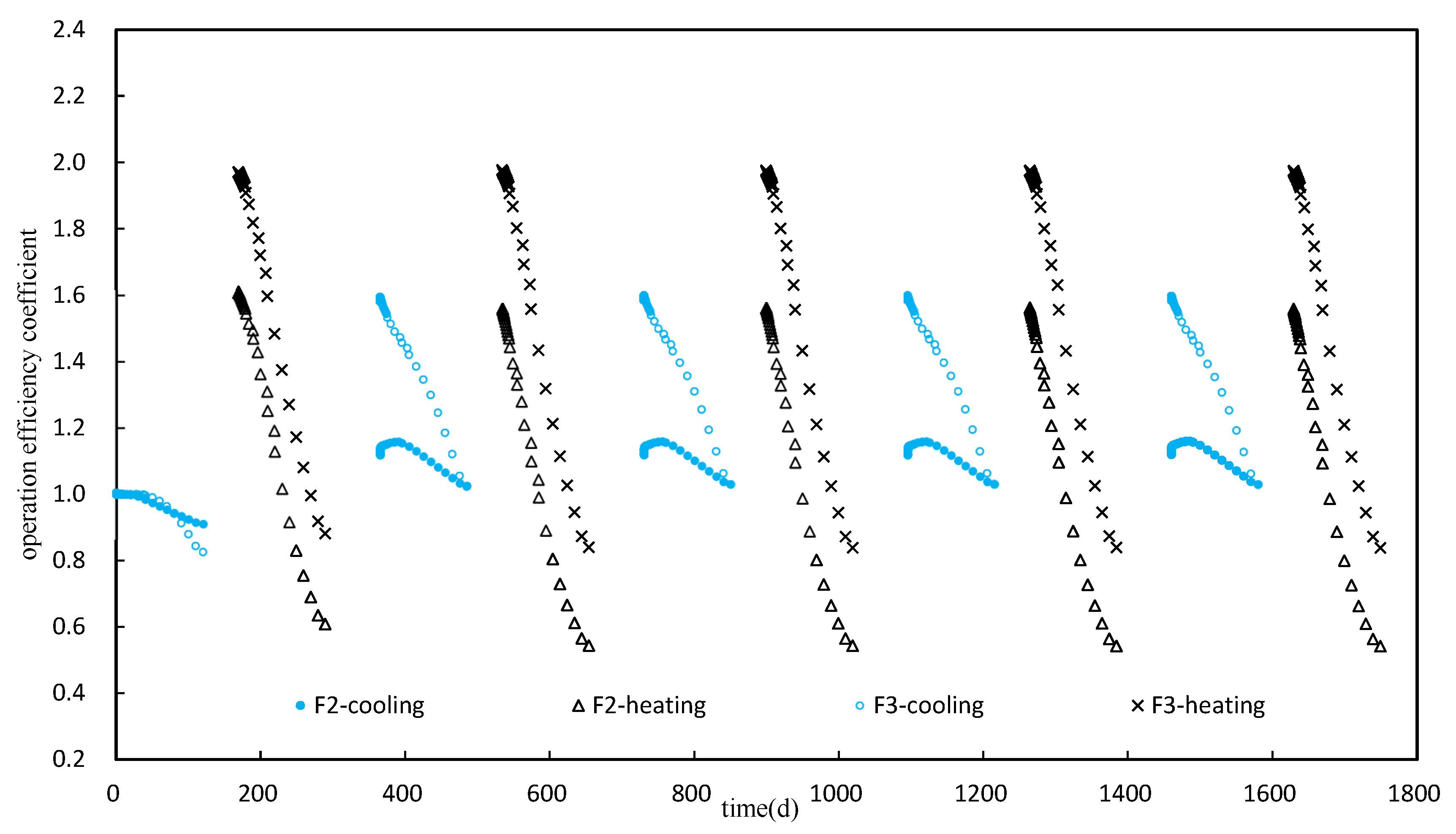
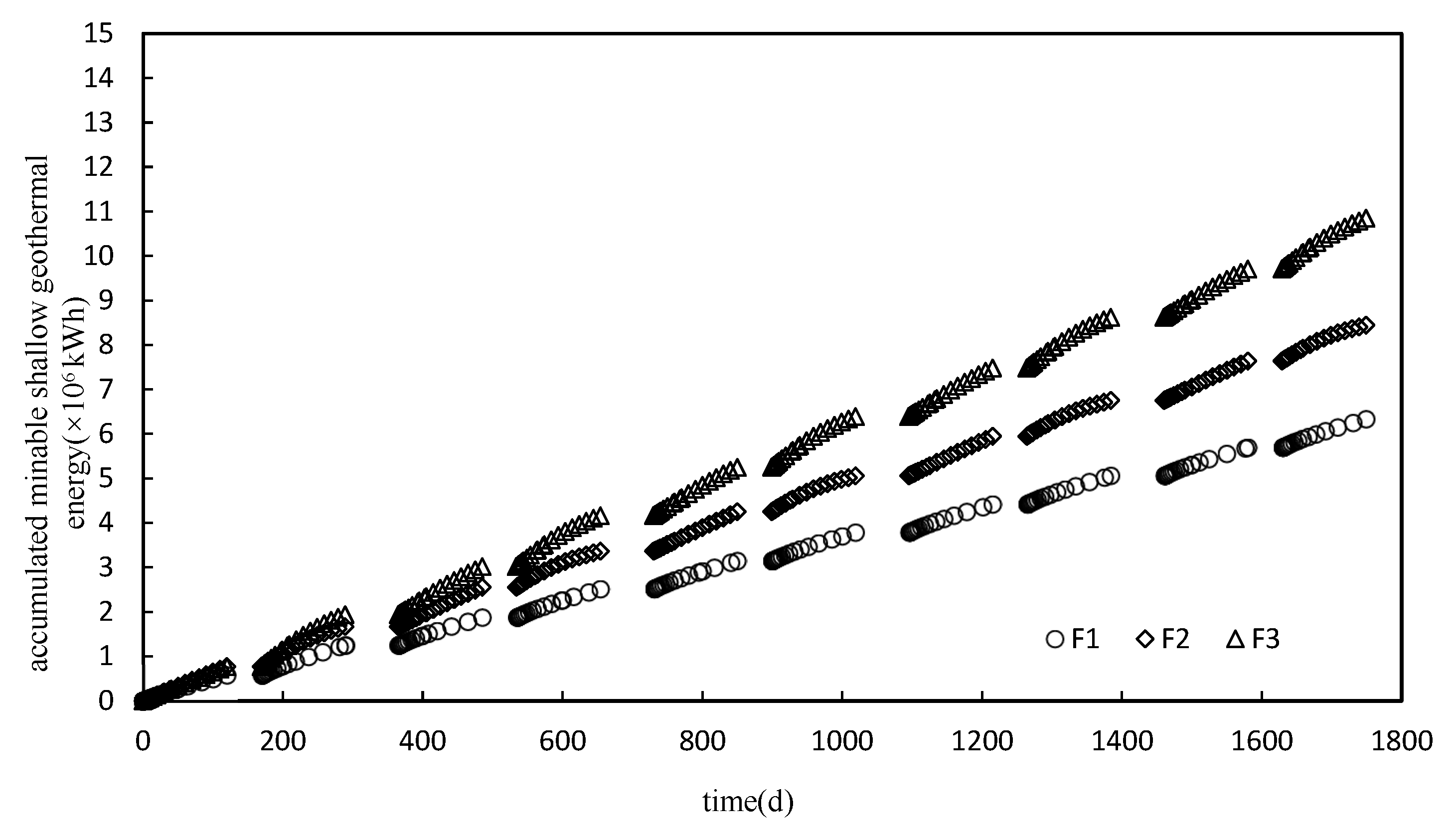
4.2.3. Evaluation of Water Source Heat Pump Operation Efficiency
5. Discussion and Conclusions
5.1. Discussion
5.2. Conclusions
Author Contributions
Funding
Institutional Review Board Statement
Informed Consent Statement
Data Availability Statement
Acknowledgments
Conflicts of Interest
References
- Wang, G.L.; Zhang, W.; Lin, W.J.; Liu, F.; Gan, H.; Fu, L. Project progress of survey, evaluation and exploration demonstration of national geothermal resource. Geol. Surv. China 2018, 5, 1–7. [Google Scholar]
- Fan, S.; Lu, Z. Research on the Peak Carbon Dioxide Emission Strategy of Chinese Port Based on Carbon Emission Estimation. Front. Environ. Sci. 2022, 9, 646. [Google Scholar] [CrossRef]
- Haehnlein, S.; Bayer, P.; Blum, P. International legal status of the use of shallow geothermal energy. Renew. Sustain. Energy Rev. 2010, 14, 2611–2625. [Google Scholar] [CrossRef]
- Ahmed, A.A.; Assadi, M.; Kalantar, A.; Sliwa, T.; Sapińska-Śliwa, A. A Critical Review on the Use of Shallow Geothermal Energy Systems for Heating and Cooling Purposes. Energies 2022, 15, 4281. [Google Scholar] [CrossRef]
- Dalla Longa, F.; Nogueira, L.P.; Limberger, J.; van Wees, J.D.; van der Zwaan, B. Scenarios for geothermal energy deployment in Europe. Energy 2020, 206, 118060. [Google Scholar] [CrossRef]
- Wenjing, L.; Qinghua, W.; Guiling, W. Shallow geothermal energy resource potential evaluation and environmental effect in China. J. Arid Land Resour. Environ. 2012, 26, 57–61. [Google Scholar]
- Hakkaki-Fard, A.; Aidoun, Z.; Ouzzane, M. Applying refrigerant mixtures with thermal glide in cold climate air-source heat pumps. Appl. Therm. Eng. 2014, 62, 714–722. [Google Scholar] [CrossRef]
- Sayyaadi, H.; Amlashi, E.H.; Amidpour, M. Multi-objective optimization of a vertical ground source heat pump using evolutionary algorithm. Energy Convers. Manag. 2009, 50, 2035–2046. [Google Scholar] [CrossRef]
- Aquino, A.; Scrucca, F.; Bonamente, E. Sustainability of Shallow Geothermal Energy for Building Air-Conditioning. Energies 2021, 14, 7058. [Google Scholar] [CrossRef]
- Drijver, B.; Willemsen, A. Groundwater as a Heat Source for Geothermal Heat Pumps. Int. Course Geotherm. Heat Pumps 1998, 2, 156–166. [Google Scholar]
- Chang, K.S.; Kim, M.J. Thermal performance evaluation of vertical U-loop ground heat exchanger using in-situ thermal response test. Renew. Energy 2016, 87, 585–591. [Google Scholar] [CrossRef]
- Liu, X.; Xiao, Y.; Inthavong, K.; Tu, J. Experimental and numerical investigation on a new type of heat exchanger in ground source heat pump system. Energy Effic. 2015, 8, 845–857. [Google Scholar] [CrossRef]
- Cui, P.; Yang, H.; Fang, Z. Heat transfer analysis of ground heat exchangers with inclined boreholes. Appl. Therm. Eng. 2006, 26, 1169–1175. [Google Scholar] [CrossRef]
- Najib, A.; Zarrella, A.; Narayanan, V.; Bourne, R.; Harrington, C. Techno-economic parametric analysis of large diameter shallow ground heat exchanger in California climates. Energy Build. 2020, 228, 110444. [Google Scholar] [CrossRef]
- Sivasakthivel, T.; Murugesan, K.; Thomas, H.R. Optimization of operating parameters of ground source heat pump system for space heating and cooling by Taguchi method and utility concept. Appl. Energy 2014, 116, 76–85. [Google Scholar] [CrossRef]
- Koroneos, C.J.; Nanaki, E.A. Nanaki. Environmental impact assessment of a ground source heat pump system in Greece. Geothermics 2017, 65, 1–9. [Google Scholar] [CrossRef]
- Luo, Z.; Wang, Y.; Zhou, S.; Wu, X. Simulation and prediction of conditions for effective development of shallow geothermal energy. Appl. Therm. Eng. 2015, 91, 370–376. [Google Scholar] [CrossRef]
- Dandan, Y.; Zujiang, L.; Yan, W.; Dezhong, Z.; Lianyu, F. Heat balance analysis and countermeasure of groundwater heat pump system of Zhengding in Hebei. J. Jiangsu Univ. (Nat. Sci. Ed.) 2015, 36, 485–490. [Google Scholar]
- Yanzhang, Z.H.O.U.; Zhifang, Z.H.O.U.; Rong, W.U. Simulation study of the stage-characteristics of groundwater thermal transport in aquifer medium for GWHP System. Hydrogeol. Eng. Geol. 2011, 38, 128–134. [Google Scholar]
- Bulté, M.; Duren, T.; Bouhon, O.; Petitclerc, E.; Agniel, M.; Dassargues, A. Numerical Modeling of the Interference of Thermally Unbalanced Aquifer Thermal Energy Storage Systems in Brussels (Belgium). Energies 2021, 14, 6241. [Google Scholar] [CrossRef]
- Russo, S.L.; Gnavi, L.; Roccia, E.; Taddia, G.; Verda, V. Groundwater Heat Pump (GWHP) system modeling and Thermal Affected Zone (TAZ) prediction reliability: Influence of temporal variations in flow discharge and injection temperature. Geothermics 2014, 51, 103–112. [Google Scholar] [CrossRef]
- Lund, J.; Sanner, B.; Rybach, L.; Curtis, R.; Hellström, G. Geothermal( ground–source) heating pumps—A world overview. GHC Bull. 2004, 9, 1–10. [Google Scholar]


| Scheme | Pumping Well | Injection Well |
|---|---|---|
| F1 | 1#, 4#, and 8#, each well with the flux of 1512 m3/d | other wells, each well with the recharge flux of 453.6 m3/d |
| F2 | In the cooling period, 4#, 6#, and 8# with the flux of 1512 m3/d, while in the heating period, 1#, 6#, and 8# with the flux of 1512 m3/d | In the cooling period, 1#, 2#, 10#, 11#, 12#, and 13# with the recharge flux of 756 m3/d, while in the heating period, 3#, 4#, 8#, 9#, and 10# with the recharge flux of 756 m3/d |
| F3 | In the cooling period, 1#, 3#, and 5# with the flux of 1512 m3/d, while in the heating period, 10#, 12#, and 13# with the flux of 1512 m3/d | In the cooling period, 8#, 9#, 10#, 11#, 12#, and 13# with the recharge flux of 756 m3/d, while in the heating period, 1#, 2#, 3#, 4#, 5#, and 6# with the recharge flux of 756 m3/d |
Disclaimer/Publisher’s Note: The statements, opinions and data contained in all publications are solely those of the individual author(s) and contributor(s) and not of MDPI and/or the editor(s). MDPI and/or the editor(s) disclaim responsibility for any injury to people or property resulting from any ideas, methods, instructions or products referred to in the content. |
© 2023 by the authors. Licensee MDPI, Basel, Switzerland. This article is an open access article distributed under the terms and conditions of the Creative Commons Attribution (CC BY) license (https://creativecommons.org/licenses/by/4.0/).
Share and Cite
Wu, Q.; Fan, Y.; Wang, X. Improvement in Operation Efficiency of Shallow Geothermal Energy System—A Case Study in Shandong Province, China. Water 2023, 15, 1409. https://doi.org/10.3390/w15071409
Wu Q, Fan Y, Wang X. Improvement in Operation Efficiency of Shallow Geothermal Energy System—A Case Study in Shandong Province, China. Water. 2023; 15(7):1409. https://doi.org/10.3390/w15071409
Chicago/Turabian StyleWu, Qinghua, Yue Fan, and Xiao Wang. 2023. "Improvement in Operation Efficiency of Shallow Geothermal Energy System—A Case Study in Shandong Province, China" Water 15, no. 7: 1409. https://doi.org/10.3390/w15071409