
Geomorphic Changes of the Scott River Alluvial Fan in Relation to a Four-Day Flood Event

Institute of Earth and Environmental Sciences, Maria Curie-Skłodowska University, 20-031 Lublin, Poland
Water 2023, 15(7), 1368; https://doi.org/10.3390/w15071368
Submission received: 11 March 2023
/
Revised: 28 March 2023
/
Accepted: 31 March 2023
/
Published: 2 April 2023
(This article belongs to the Special Issue Fluvial Systems and River Geomorphology)
Abstract
:A four-day glacier-melt flood (13–16 August 2013) caused abrupt geomorphic changes in the proglacial gravel-bed Scott River, which drains the small (10 km2) Scott Glacier catchment (SW Svalbard). This type of flood occurs on Svalbard increasingly during periods of abnormally warm or rainy weather in summer or early autumn, and the probability of occurrence grows in direct proportion to the increase in temperature and/or precipitation intensity. In the summer of 2013, during the measurement season, the highest daily precipitation (17 mm) occurred on 13 August. During the following four days, it constituted in total 47 mm, i.e., 50% of the precipitation total for the measurement period of 2013. The largest flood in 20 years was caused by high precipitation with a synchronous rise in temperature from about 1.0 to 8.6 °C. These values exceeded multi-year averages (32 mm and 5.0 °C, respectively) at an average discharge of 0.9 m3/s (melt season mean 1986–2011). These conditions caused a rapid and abrupt response of the river with the dominant (90%) glacier-fed. The increase in discharge to 4.6 m3/s, initiated by the glacial flood, mobilized significant amounts of sediment in the river bed and channel. Geomorphic changes within the alluvial fan as an area of 58,940 m2, located at the mouth of the Scott River, were detected by multi-sites terrestrial laser scanning using a Leica Scan Station C10 and then estimated using Geomorphic Change Detection (GCD) software. The changes found involved 39% of the alluvial fan area (23,231 m2). The flood-induced total area of lowering (erosion) covered 26% of the alluvial fan (6035 m2), resulting in the removal of 1183 ± 121 m3 of sediment volume. During the final phase of the flood, two times more sediment (1919 ± 344 m3) was re-deposited within the alluvial fan surface, causing significant aggradation on 74% of its area (17,196 m2). These geomorphic changes resulted in an average lowering (erosion) of the alluvial fan surface of 0.2 m and an average rising (deposition) of 0.1 m.
1. Introduction
The intensity of fluvial processes shaping valley floors is a sensitive indicator of contemporary geomorphic changes in the cold climate environment [1]. The erosion–deposition processes occurring in the Arctic river catchments reflect the coupling between sediment sources, valley bottoms and river channels [2]. The rate of these changes is usually assessed by estimating the sediment yields and the relationship between the river transport components [3,4]. Regional and local conditions determine the high variability of total sediment yields from glaciated (600~40,000 t/y) and unglaciated (500–1000 t/y) catchments of the polar regions [5]. The main determining factors include the rate of glacier and snow cover ablation and the frequency of different genesis floods [6,7,8]. For high Arctic proglacial rivers, the dominance of suspended sediment transport is characteristic, constituting up to 80% of sediment yields (while the bedload is up to 37%) [5,9]. The local character and episodic nature of the coarse sediments delivery to the channels of Arctic rivers makes the bedload discharge show higher temporal and spatial variability than the suspended load discharge [5,10]. The rate of bedload and its relationship to other components of fluvial transport (suspended and dissolved loads) determine changes in valley floor and channel morphology [11,12]. Significant geomorphic changes of the valley floor and channel can be a result of even a single flood episode [13,14]. Quantitative assessment of bedload transport, including the identification of its sources and routes of distribution, as well as transport and deposition, are essential for assessing contemporary trends of high-Arctic valley floor development [15,16].
The objective challenges of conducting direct measurements of river bedload transport, in cold climate environments [17,18,19], has resulted in a relatively small number of studies. However, those that are available emphasize the morphogenetic role of the bedload in the contemporary development of valley floors [10,12,20,21,22]. Studies of the modern development of river valleys located in high latitudes and high mountainous areas have so far focused on assessing the spatial distribution of sediment storage types and quantification [23], sediment budgeting [5] and identifying their sources and routes of delivery [2,9,24,25] as well as assessing the rate and directions of bed and channel reshaping [26]. With the increasing access to remote sensing data, studies of fluvial transport are being supplemented by assessments of geomorphic changes of high-Arctic river valleys carried out on the basis of morphometric analyses based on high-resolution elevation models. Of the remote sensing techniques commonly used to study changes in the relief of high-Arctic valleys [27], the most effective are Light Detection and Ranging (LiDAR) methods including airborne (ALS) and terrestrial laser scanning (TLS). ALS-derived data are characterized by much higher resolution than satellite data (up to several pt/m2) [28,29,30,31]. The high-resolution digital elevation models (DEMs) developed from them provide a good base for differential comparative analyses (DEM of Difference), which results in quantitative estimates of geomorphic changes [32,33,34]. However, ALS has significant limitations, which are mainly related to the high cost of the flight. Because of this, TLS-derived data [2,24] or structure-from-motion (SfM)-based UAV-derived photogrammetric data [35] become the basis for short-term changes. Extreme weather conditions such as intense precipitation or a significant increase in air temperature (or both occurring at the same time) can cause considerable geomorphological results, although the resulting development of landforms is often ephemeral and quickly damaged [36]. In the case of extreme events with an incidence of 10 or 20 years, the entire valley floor can be reshaped, and the river channels change position as a result of overtopping [2]. In such cases, the use of TLS provides a high efficiency of change detection [37,38]. Dense 3D point clouds obtained through it, and high-resolution digital terrain models (DTMs) based on them, allow for the estimation of changes in the surface and geometry of landforms [39], landform typology [40] or interpretation of landform development [41]. In the river valley systems of cold climate environments, alluvial fans play a very important role. Their specific status is related to both their location and their different morphology [42]. They are located in the lower/mouth section of the valley floor, and their fan-like shape is the result of increased deposition of river loads at the point where the bed slope changes and the river loses its velocity and transport energy [43,44,45]. Floods and the depositional processes that are activated during the flooding have a considerable impact on the development of alluvial fans [46]. During floods, the increased volume and velocity of water can cause the erosion and redistribution of sediments [10], causing changes in the size and shape of the fan [47]. Moreover, the energy of the flow increases greatly, and the river gains the ability to redeposit large amounts of bedload, which after a short transport is deposited on the surface of the fan, further modifying its relief [48]. As a result, the landforms of the valley floor (lateral, longitudinal bars) and the channel (bank erosion) are reshaped [2,12]. Above-average floods lead to the abandonment of previous channels and the creation of new ones or the widening and deepening of existing ones, which can cause changes in the overall drainage pattern of the alluvial fan [2,49].
The goal of this study is to indicate the importance of extreme hydro-meteorological events in the transformation of the floors of high-latitude proglacial valleys. To achieve this, a multidimensional estimation of short-term geomorphic changes in the alluvial fan of the proglacial gravel-bed of the Scott River, which occurred as a result of an extreme four-day flood caused by the coupling of high precipitation and a rapid increase in air temperature, was carried out. Detection of changes based on TLS-derived data and the high-resolution digital terrain models (DTMs) generated from them was carried out using the DoD method taking into account the surface level of the alluvial fan immediately before and after the flood. As a result, the range of changes in the fan surface was mapped, and their quantitative characteristics and sediment budget were obtained, which allowed comparison to changes over a three-year interval.
2. Materials and Methods
2.1. Study Area
The study of geomorphic changes in the alluvial fan of a proglacial gravel-bed Arctic river was carried out in the catchment area of the small Scottbreen glacier valley. Taking its source from the glacier, the Scott River is located in the northwestern part of Wedel-Jarlsberg Land (southwestern Svalbard) (Figure 1A), adjacent to Bellsund Bay in the north and Recherche Fjord in the east (Figure 1B). The study site is located in the northern part of Sør-Spitsbergen National Park (Figure 1A), where 65% of the area is covered by glaciers. The catchment area of 10.1 square kilometers (km2) is more than 40% covered by a valley glacier (alpine type) about 3 km long (Figure 1B).
The highest parts of the glacier reach ~600 m above sea level (m a.s.l.), while the glacier’s mouth reaches ~92.5 m a.s.l. The unglaciated part of the 3.3 km-long valley [22] is drained by the proglacial Scott River. It is a typical gravel-bed river with a glacial regime, where the dominant (90%) source of water is melting glacier [50].
Moreover, along the unglaciated section, the river is also fed by small tributaries, and its spatial pattern is characterized by a variable channel system (Figure 1B) [19]. The Scott River alluvial fan has developed below a narrowing gorge located in the lower section of the unglaciated valley floor. Widening eastward, the fan-form occupies an area of 0.06 km2 (Figure 1C). The difference in elevation between fan-head and fan-toe is 5.3 m (from 5.8 to 0.5 m above sea level). The length of the fan between these points is about 300 m, and its maximum width is 450 m. The alluvial fan’s drainage channel system is located mainly in its northern part. The blocking of the fan by the coastal rampart of the Recherche Fjord forces a change in direction of the outflow of the main channel, creating a small lagoon in the NW part from which water is discharged along the fan-toe to the SE. The central and southern parts of the surface of the alluvial fan are covered by a network of distributary channels that fill with water only during the largest floods (Figure 1C).
2.2. Meteorological and Hydrological Measurement
The hydro-meteorological background of the glacial-melt flood between 13 and 16 August 2013 was determined on the basis of continuous measurement stations recording changes 144 times a day. The meteorological conditions of the event (air temperature, precipitation totals, wind direction and strength) were monitored at 10-min intervals using an automatic weather station located on an elevated marine terrace (23 m above sea level) about 200 m from the Recherche Fiord coastline (next to the Maria Skłodowska-Curie University (MCSU) research station). Changes in the water stage and flow velocity of the Scott River were measured at two hydrometric gauges located above the fan-head and in the fan-toe drainage channel (Figure 1C). The first hydrometric profile was located in the gorge cutting through the elevated marine terraces about 350 m above the river’s mouth at Recherche Fjord [51]. The valley floor narrows here to about 50 m, and the Scott River converges the braided channels into one for most of the snow-melting season [2]. The second hydrometric profile was located in a channel that receives water from an alluvial fan about 100 m from the river’s mouth at Recherche Fjord (Figure 1C). Changes in water levels were measured using Schlumberger electronic limnigraph also at 10-min intervals. River flow was determined using a rating curve equation developed from flow velocity measurements taken twice a week with a Hega II type current meter and, in addition, an Acoustic Digital Current Meter (OTT ADC).
2.3. High Resolution Surveying: TLS-Derived Digital Terrain Models (DTMs)
The study used data from three campaigns of high-accuracy surveys of changes in the alluvial fan surface of the Scott River. During the 2013 snow-melting season (and also 2010), TLS surveys were taken at a 3-week interval in late July and on 18 August 2018. High-precision TLS surveys were performed using a Leica Scan Station C10 terrestrial laser scanner (Figure 2).
It is a 300 m range scanner that pulses a green laser beam (532 nm) at 50,000 points per second (pt/s) [52]. The acquired data were also compared to measurements taken in July 2010. During the 2010 and 2013 campaigns, different techniques were used to record individual scans and georeference the resulting models [53]. In 2010, scans of the survey area were taken in a local reference system, and individual scans were registered to a minimum of three common reference points on which black and white Leica targets were located. Registration of the scans to a unified model was completed in Cyclone 8.1 ®Leica software (Leica Geosystems AG, Heerbrugg, Switzerland). The georeferences of the model were given based on measurements of five reference points by Leica 500 dGPS with an accuracy of 0.02 m. In 2013, a different approach was used to register the scans and attribute georeferences to them. In the pre-TLS survey period, a network of solid reference points was set up in the valley floor and slopes in the type of wooden stakes driven into the ground with a marked center point. Subsequently, the positioning of all network points was carried out using TopCon Hiper II dual-frequency GNSS receivers (GPS+GLONASS; Global Positioning System (GPS) and Globalnaja Nawigacionnaya Sputnikovaya Sistiema (GLONASS)). A base-rover measurement method was used, which made it possible to determine the real-time position of network points with an accuracy of 0.02 m. A network of reference points was used to locate the scanner and target points on which one black and white Leica target were located. Information about the coordinates (x,y,z) of the network points was imported into the measurement project directly in the scanner interface as a text file. This allowed the coordinates of the scanner’s position to be determined before measurement data acquisition. As a result, the entire point cloud acquired at each measurement position had georeferences automatically assigned. The method of scanning from a point with ‘known coordinates’ significantly reduced the time of field work and the data processing stage in post-processing (Figure 2).
2.4. Ground Point Classification and Development of DTMs
Survey data from each campaign were integrated into a unified digital surface model (DSM) using Cyclone 8.1 ©Leica software (Figure 2). The resulting point clouds were then classified to obtain ground points. Classification was performed automatically using the Cloth Simulation Filter (CSF) algorithm [54] and then manually to remove artifacts missed by the algorithm [53] (Figure 2). The CSF algorithm used was implemented as a plug-in for CloudCompare 2.11, and the following parameters were used: slope processing was set to ‘active’; ‘Cloth’ resolution was set to 0.1 m; number of iterations 1000; classification threshold 0.1 m. In the ‘Cloth’ parameters, the lowest available parameter size was used. The manual ‘cleaning’ of ground points was carried out in Leica Cyclone 8.1 software using the ‘limited fence’ function in the ‘view’ module. The point clouds selected as ground points were transformed into DTMs using LP360 7.0 software (©GeoCue 520 6th Street Madison, AL 35756, USA) (Figure 2). Each of the three DTMs was transformed into a triangulated irregular network (TIN) and then rasterized as a GeoTIFF with a resolution of 0.1 m.
2.5. Determination of the Extent of the Flood: Photo Rectification
Assessment of the geomorphic changes that occurred as a result of the direct impact of flood waters required determining their maximum extent within the surface of the alluvial fan. On 17 August, during the peak of the flood wave, diagonal images of the study area were taken with a Canon EOS D60 digital camera (Figure 2). The images were taken for the entire alluvial fan with 40% coverage of the of the next image (Figure 3A). The images were taken from the edge of a raised marine terrasse elevated 25 m above the surface of the fan (Figure 1C). Processing of the images into cartometric form and mapping in the field coordinate system was carried out using Agisoft software (©Agisoft LLC, St. Petersburg, Russia) (Figure 2). The rectified fan imagery was then overlaid on the DTM in ArcGIS 10.8 software (Figure 3B). In order to correct errors related to lens distortion, a transparency of 50% was applied to the model visualization. This allowed the extent of the flooded area during the flood to be corrected for fan relief. The extent of the flooded and water-free areas was drawn in ArcGIS 10.8 as polygons, which were then used to make ‘masks’ used further in DoD analyses to constrain the area of interest (AoI) (Figure 2).
2.6. Detection of Surface Changes by DEM of Difference (DoD)
To obtain information on the geomorphic change extent of the alluvial fan surface, DTMs were analyzed using the Geomorphic Change Detection software version 7.4.4 (GCD) plug-in for ArcGIS 10.8 software (Figure 2). Following the guidelines of the author of the DoD method [33,55], an approach based on the uncertainty range based on the minimum level of detection (min-LoD) was used. In the case of TLS measurements, the measurement error is related to the accuracy of the rangefinder (for ScanStation C10, it is ~0.006 m at a distance of up to 50 m) [52]. When registering the scans of the 2010 survey campaign, it was assumed that the error could not exceed 0.009 m. The largest error was associated with GNSS position fixing (0.02 m). Similarly, in the 2013 campaign, the error of the rangefinder was the same; here, the georeferencing step in post-processing was omitted (no associated error), but at the same time, the largest error (0.02 m) was associated with the positioning of the reference network. As a result, it can be assumed that the use of exactly the same reference points in both 2013 campaigns resulted in a non-error reduced to the uncertainty associated with rangefinder accuracy, but in all three surveys, the largest uncertainty is associated with the positioning error underlying the georeferencing of all three DTMs. Therefore, a minLoD of 0.02 m was assumed in the DoD analysis. An area-of-interest (AoI) ‘mask’ was used for all three models compared, limiting change detection to the alluvial fan area only (58,940 m2).
3. Results
3.1. Hydrometeorological Background of the Four-Day Flood from 13 to 16 August, 2013
The 2013 melting season was generally slightly warmer (daily average of 5.9 °C) than the multi-year average (4.5 °C). Extreme temperatures occurred in the period preceding and following the flood event. The lowest average daily temperature was 2.7 °C (13 August), while the highest was 8.6 °C (17 August) (Figure 4). During the same period, the significant increase in temperature was coupled with above-average precipitation totals. The total precipitation on four consecutive days (13–16 August) amounted to 46.9 mm, while the highest 16.8 mm was recorded on August 14. The four-day precipitation sum accounted for 43% of the total precipitation in the analyzed summer season of 2013. The increased precipitation–ablation supply resulted in a significant increase in flow velocity and consequently the largest flood recorded since 1992 [51]. Franczak et al. [56] estimated that the discharge of the Scott River increased during this event from 0.74 m3/s (12 August) to 4.63 m3/s on 16 August (Figure 4). The estimated peak flow during the flood exceeded 10 m3/s, which relates to the rate estimated by Bartoszewski [51] for a flood recorded 20 years earlier in the Scott River in 1992.
3.2. Geomorphic Implications of the Four-Day Flood between 13 and 16 August, 2013
Analysis of the differences in the alluvial fan area of the Scott River pre- and post-flood event conducted using GCD software [32,33,55] allowed the quantitative estimation (Table 1) and mapping of changes in its boundaries (AoI). The results of comparing DTMs from the three-week period of late July and 18 August 2013 show significant differences in the transformation of the fan area (Figure 5). The total area analyzed in the AoI-limited range was 58,940 m2, of which detectable changes affected 23,231 m2, which is 39% of the fan area. Surface height decrease was found on 10% of the AoI, while the percentage for the area of detectable changes was 26% (Table 1).
Almost three times the area of AoI was elevated. This was 29% of AoI and 74% of the area undergoing change, respectively. The change in surface elevation reflects the effects of erosion and deposition processes on the surface of the alluvial fan during the flood. Quantitative summaries of these changes are given with the threshold value. The lowering of the surface, which was a direct result of depressional and lateral erosion, resulted in the removal of 1183 ± 121 m3 of sediment. In contrast, deposition resulted in an increase of 1919 ± 344 m3 of sediment. The sum of the volume of lowering and raising is 3102 ± 465 m3, while the difference in the volume of deposition and erosion is 736 ± 364 m3. In accordance with the changes in elevation expressed in terms of the average change in height/depth, erosional processes had greater dynamics than dispositional ones. Recorded for the change detection area, the average depth of surface lowering was 0.2 ± 0.02 m, while for deposition, it was twice as low.
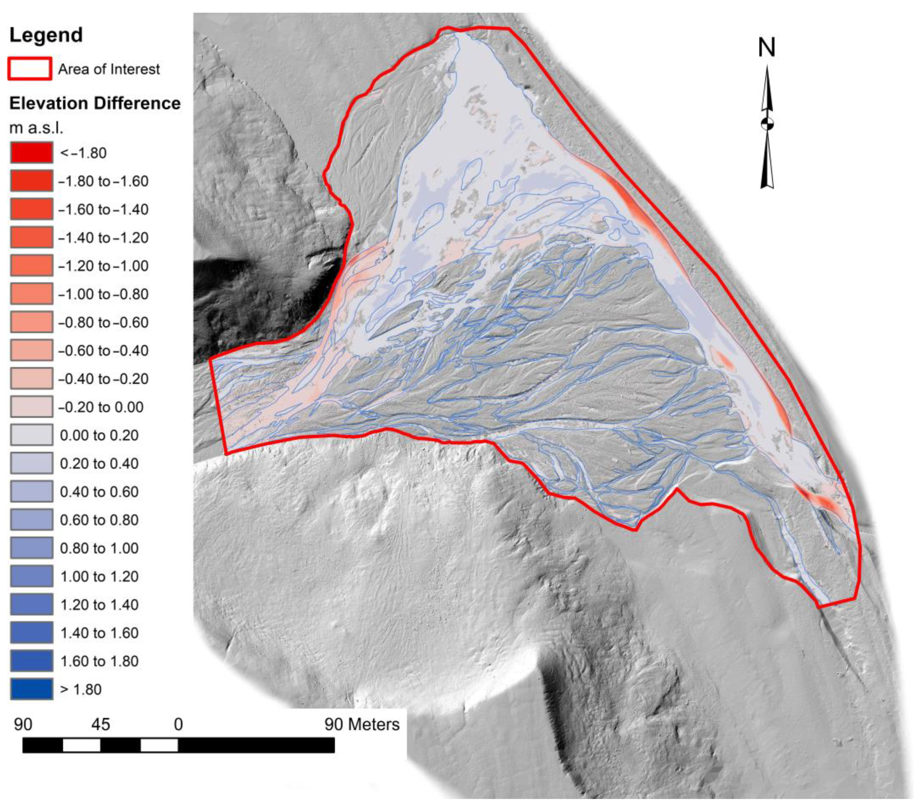
The map of changes in the surface of the alluvial fan caused by the flood event shows spatial diversity in their extent and dynamics (Figure 5). In general, the changes covered the northern and eastern parts of the fan, with the greatest diversity occurring along the boundaries of the feeder channel. In the fan-head and along the fan-toe, erosion predominates, while on the northern side of the fan, deposition predominates. The greatest erosion dynamics covers the slopes of the northern part of the gorge mouth and the inner slopes of the coastal rampart (Figure 5).
The dynamics of surface changes were also analyzed for the entire flooded area (21,755 m2; 37% of the alluvial fan area) during the flood peak (Table 2). Detectable changes (threshold value) covered 16,187 m2, representing 28% of the fan area and 74% of the AoIFA flooded area (flooded area). Lowering of surface elevation was found in 23% and raising was found in 77% of the AoIFA (Table 2).
Lowering the surface resulted in the removal of 880 ± 73 m3 of sediment, while deposition resulted in the addition of 1463 ± 250 m3 of sediment. The sum of lowering and raising volumes was 2342 ± 324, while the difference in deposition and erosion volumes was 583 ± 261 m3. The average change in elevation was slightly greater than that for the entire fan, and it was 0.24 ± 0.02 m for erosion, while for deposition, it was twice as low, respectively. Spatially, the changes were concentrated in the feeder channel. The greatest dynamics of erosion processes can be seen at the mouth of the gorge, where the main stream moves from under the southern slope toward the northern one, undercutting it intensively in the vicinity of the shoreline (Figure 6). After passing the undercut slope, the flooded area widens considerably, covering much of the northern wing of the fan. Deposition prevails here. Intense lateral erosion also covers the eastern slope of the channel draining the Scott River into the Fjord. The coastal rampart has shifted back locally by up to 4 m here. However, as a result of deposition, the riverbed has become shallower and wider in this part. Less dynamic changes were registered in the periodically activated distribution channels (Figure 6).
A much smaller range of surface changes was found in the non-flooded or briefly flooded areas (37,110 m2; 63% of the alluvial fan area) (Table 3). Detectable changes (threshold value) covered only 7032 m2, which is 12% of the fan area and 19% of the non-flooded area (AoINFA). The effects of flooding were much more balanced here. Surface elevation lowering was found in 34% and raising in 66% of AoINFA (Table 3).
Despite the almost twofold advantage of raised versus lowered area, the relationships of sediment volume removed 303 ± 47 m3 and deposited 456 ± 93 m3 are similar. Likewise, the average change in elevation (lowering) of 0.13 ± 0.02 was slightly greater than that of raising 0.11 ± 0.02. Spatially, the greatest dynamics of erosion and disposition processes can be seen in the bars and inter-channel islands located at the mouth of the gorge and in the neighborhood of the main stream. At the mouth of the gorge, erosion is predominant, while deposition is predominant on the rest of the bars (Figure 7).
The study also analyzed changes in the area of the alluvial fan during the three-year interval 2010–2013 (Figure 8). During this period, detectable changes covered 57,125 m2, representing 97% of the fan area. The predominant surface elevation lowering was 88% of AoI and 91% of the area of detectable changes (Table 4). Almost ten times less AoI area was elevated (9%). Such a significant predominance of lowered areas resulted in the removal of 7543 ± 1040 m3, i.e., about seven times more than during the four-day flood of 2013. In turn, the volume of sediment deposited during the three-year period, 875 ± 102 m3, was twice as small as that deposited during the flood episode. The average change in elevation (downcutting) of 0.14 ± 0.02 was slightly less than the uplift of 0.17 ± 0.02 (Table 4). Spatially, the dynamics of erosion and deposition processes are similar to the range shown in Figure 7. The difference can be seen mainly in the non-flooded areas, which were subject to downcutting during the three-year period (Figure 8).
4. Discussion
4.1. Extreme Hydrological and Meteorological Events
Observations of floods of various provenance in the Scott River catchment indicate that events of thermal and precipitation–thermal genesis are the most common [50,51,56,57,58,59]. The primary determinant of runoff is air temperature, which affects the rate of glacier ablation. Its strong relationship with outflow has been statistically documented [56]. These authors have also shown that the amount of precipitation is of less importance, although the largest discharges (including flood discharges) are usually initiated by a combination of both factors simultaneously [56]. It is also important to emphasize the important role of fen-type winds from a southerly direction, which, floating on the surface of Scottbreen Glacier, enhance the thermal effect and mobilize widespread runoff from the entire glacier surface [35,56]. In August 2013, this type of hydrological event was recorded for the first time in 20 years [51]. This extreme flooding was caused by the simultaneous occurrence of an increase in air temperature and intense rainfall in a four-day interval [56], which also confirms other authors’ studies conducted in the Scott River [50,51].
The occurrence of weather extremes in a very short period of time can considerably change runoff conditions in the glacial catchments of Spitsbergen, as reflected in the high variability of fluvial transport [10] and the reshaping of the valley floors [2]. Of all the components of the total sediment yield, bedload plays the greatest role with the change in the morphology of valley floors and river channels of the cold climate environment [1,4,5,9,14,20]. The fluctuating nature of bedload is a characteristic of its transport mechanism [5,11], and the crucial factor in the amount of sediment discharged are floods [13], during which up to 70-90% of bedload is discharged [5]. In the Scott River catchment, the largest amount of bedload is transported during floods of ablation–rainfall genesis. In 2009–2013, the share of maximum daily loads recorded during flood episodes was up to 30% of the seasonal bedload discharge. Floods of an ablation–rainfall genesis are rarely recorded in the second half of the melt season. However, when they do occur, their course is sometimes very rapid [51]. Examples of such events in August (2012, 2013) show that the morphological effects are significant for the formation of the alluvial fan surface [48]. They coincide with the period of maximum thickness of the active permafrost layer, so both the slope and bottom material can be easily mobilized and redeposited [10].
4.2. TLS-Derived DTMs Analysis
Remote sensing methods are currently a source for acquiring high-precision elevation data for the development of digital terrain models of DTMs [30]. High-Arctic areas are a particularly favorable area for their application [60]. On the one hand, harsh climatic conditions limit the possibility of direct field measurements [24]; on the other hand, the almost complete absence of vegetation cover and infrastructure objects facilitates the development of terrain models [53]. The detailed geomorphology of alluvial fans in the high-Arctic periglacial environment, among others, has been the subject of a study using Unmanned Aerial Vehicle (UAV) surveys [59]. Analyses based on TLS-derived DTMs in the Scott River drainage basin have involved survey methodologies [24], estimation of sediment sources, identification of sediment delivery and redeposition pathways into non-valleys [2,24], the use of geomorphons to analyze changes in glacial valley morphology [40], but also an estimation of geomorphic changes in glacier forelands [36] and non-glacial valley floors [26].
The applied methodology permits the quantitative estimation of geomorphic surface changes occurring both as a result of single hydrometeorological events and medium-term changes [2,26]. Accurate estimation of the range, spatial diversity and dynamics of these changes requires consideration of three potential sources of uncertainty: (i) the accuracy of the measuring equipment, (ii) the methodology of surveying, recording and georeferencing, (iii) the methods of ground point classification and DTM transformation [24]. The results show that the applied methods of field measurements and processing of measurement data in post-processing including the filtering of ground points with the CSF algorithm have high efficiency [53]. The study uses a range of MinLoD = 0.02 m, referring to the accuracy of GNSS positioning during field measurements [2,24]. Of the measurement devices used, it is the satellite positioning system that has the highest conceivable error. Both the accuracy of the 3D position measurement by the scanner (0.006 mm at a distance of 50 m) [52] and the registration of scans (1 −0.01 m) affect the measurement uncertainty to a much lesser extent. Other parameters related to point cloud classification by CSF and the generation of DTMs are of much lower importance [53]. Setting MinLoD = 0.02 m resulted in the detection of active changes found in about 40% of the AoI area (Table 1). This value is close to the share of the area determined from digital images as the area flooded during the peak of the flood. It accounted for 37% of the area of the studied alluvial fan (AoI).
The study showed that the alluvial fan surface of the Scott River can be significantly transformed both episodically (during single extreme events) and over several years. This confirms the observations of Pasternack and Wyrick [14] on the role of floods in the contemporary shaping of the valley floor.
The results of the measurements showed a high spatial diversity of the detected geomorphic changes and processes shaping the surface of the alluvial fan. The role of the feeder channel and the area under flooding was highlighted as well as the change in trend from the predominance of erosional processes near the fan-head to depositional processes in the middle and lower parts of the fan. This change in trend confirms that the Scott River fits well into the general model of alluvial fan development [42,43]. Due to the change in valley slope from 0.016 to 0.008 below the constriction of the gorge [2], the river has the freedom to spill and distribute water over the surface of the alluvial fan. This is also confirmed by multi-season bedload transport studies in the Scott River. Measurements in cross-sections located above the fan-head and in the channel receiving waters from the fan-toe show a general decrease in bedload, indicating the deposition of some sediment on the cone surface. This occurs as a result of a decrease in the carrying capacity of the river and becomes the direct cause of the differences in bedload discharge found [48]. In accordance with the analyses of geomorphic changes in the surface of the Scott River alluvial fan based on DoD TLS-derived DTMs over a three-year period (2010–2013), erosion prevails both in terms of area and sediment volume, and the surface lowered by an average of 0.14 ± 0.02. Changes found during the four-day flood in August 2013 show the opposite trend. Deposition predominated over most of the fan area, and the study area was raised by an average of 0.11 ± 0.02 m. Analysis of the geomorphic effects of this flood, the largest since 1993 [51], the course of which was recorded in this part of the Wedel–Jarlsberg Land, indicate that above-average hydro-meteorological events with a rapid progression can radically change the trend from erosion to aggradation.
5. Conclusions
- Environmental changes due to extreme climatic events are of broad interest to the international scientific community. The cold climate environment is particularly sensitive to these changes, and river valleys are a responsive indicator of these adjustments. The development of alluvial fans located in the mouth sections of valleys reflects the evolving dynamics of processes reshaping the catchment area. Therefore, it is important to monitor these changes based on modern measurement technologies and methods for the quantitative estimation of these changes.
- The alluvial fan of the proglacial gravel-bed Scott River is an interesting research case study of geomorphic changes in river valleys. The study area was covered three times by high-resolution TLS surveys. Two of these campaigns were performed over a three-week period in late July and early August 2013 and recorded the changes that occurred on the fan surface as a result of a four-day flood, which was the largest hydro-meteorological event in 20 years. TLS-derived DTMs made it possible to assess the quantitative changes and their spatial diversity. Analysis of the dynamics of geomorphic processes shaping the surface of the alluvial fan provided a basis for tracing the short-term and medium-term transformation of the landform of this part of the valley under conditions of progressive degradation of the glacial catchment cryosphere in a sensitive cold climate environment.
- Two areas differing in the range of changes and dynamics of geomorphological processes were identified: (i) the area undergoing flooding during the peak of the flood and (ii) the area not being flooded or briefly flooded. In the first one, a change in the trend from erosion to aggradation increasing as one moves away from the fan-head was found. A map of the spatial diversity of these geomorphic changes indicates that the range of sediment transport by floodwaters is limited. Much of the sediment eroded in the upper part of the fan-head is deposited on the northern wing of the fan. The coastal rampart along the fan-toe was also eroded laterally (up to more than 4 m). In the not-flooded area, the range of changes was much smaller.
- A comparison of the 2010 and 2013 DTMs showed that on a very short time scale, rapid meteorological events can cause changes in the relief of the alluvial fan radically different from the rate and direction of annual and multi-year changes. Net changes in sediment volume over the entire fan area in the 2010–2013 three-year period amounted to −6669 ± 1045 m3 (predominance of erosion) while during the described flood event in 2013, it was 736 ± 364 m3.
- The analysis of geomorphic changes in the alluvial fan carried out can contribute to a better understanding of how modern processes shape the lower sections of proglacial gravel-bed rivers. Detailed comparative analyses have confirmed the high accuracy and effectiveness of high-resolution TLS-derived DTMs as a tool for inventorying and tracking the high-dynamic development of river valley bottoms. The methodology used in this study to perform both measurements and comparative analyses on high-resolution models of the study areas is effective and universal, and it should also be used to complement traditional methods of measuring river sediment yield.
- The technological progress has made LiDAR-derived data more widely available and increasingly used for evaluating environmental changes. Multi-site high-accuracy TLS surveys are an effective source of comparative data, but they are burdened by the need for time-consuming field measurements. The possibility of using Unmanned Aerial Vehicles (UAVs) means that contemporary multi-site TLS surveys are increasingly being replaced by UAVs equipped with LiDAR sensors. Despite the lower surveys’ accuracy, the use of these techniques gives us the ability to detect changes in real time.
Author Contributions
Conceptualization, W.K.; methodology, W.K.; software, W.K.; validation, W.K.; formal analysis, W.K.; investigation, W.K.; resources, W.K.; data curation, W.K.; writing—original draft preparation, W.K.; writing—review and editing W.K.; visualization, W.K.; supervision, W.K.; project administration, W.K.; funding acquisition, W.K. All authors have read and agreed to the published version of the manuscript.
Funding
The study was supported by: the scientific project of the National Science Centre 2011/01/B/ST10/06996 ‘Mechanisms of fluvial transport and sediment supply to channels of Arctic rivers with various hydrological regimes (SW Spitsbergen)’ and the statutory research of FESSM MCSU ‘Application of the TLS in the geomorphological research’.
Data Availability Statement
The data presented in this study are available on request from the corresponding author.
Acknowledgments
The study was carried out in the Scott River catchment in the summer season of 2013 with the participation of the University of Maria Curie-Skłodowska’s Polar Expeditions Team. The author would like to thank the reviewers for their valuable comments that helped to make the improvements that were essential to the successful completion of this work. The author are also grateful for the English language proofreading by Andrew Warchoł.
Conflicts of Interest
The author declare no conflict of interest.
References
- Beylich, A.A.; Warburton, J. (Eds.) Analysis of Source-to-Sink Fluxes and Sediment Budgets in Changing High-Latitude and High-Altitude Cold Environments: SEDIFLUX Manual, 1st ed.; Norges Geologiske Undersokelse: Trondheim, Norway, 2007; p. 158. [Google Scholar]
- Kociuba, W. Assessment of Sediment Sources throughout the Proglacial Area of a Small Arctic Catchment Based on High-Resolution Digital Elevation Models. Geomorphology 2017, 287, 73–89. [Google Scholar] [CrossRef]
- Warburton, J. An Alpinie proglacial fluvial sediment budget. Geogr. Ann. 1990, 72, 261–272. [Google Scholar] [CrossRef]
- Beylich, A.A.; Kneisel, C. Sediment budget and relief development in Hrafndalur, subarctic oceanic Eastern Iceland. Arct. Antarct. Alp. Res. 2009, 41, 3–17. [Google Scholar] [CrossRef]
- Orwin, J.F.; Lamoureux, S.F.; Warburton, J.; Beylich, A.A. A framework for characterizing fluvial sediment fluxes from source to sink in cold environments. Geogr. Ann. 2010, 92, 155–176. [Google Scholar] [CrossRef]
- Arheimer, B.; Lindström, G. Climate impact on floods: Changes in high flows in Sweden in the past and the future (1911–2100). Hydrol. Earth Syst. Sci. 2015, 19, 771–784. [Google Scholar] [CrossRef] [Green Version]
- Carrivick, J.L.; Rushmer, L. Understanding high-magnitude outburst floods. Geol. Today 2006, 22, 60–65. [Google Scholar] [CrossRef]
- Taylor, C.; Robinson, T.R.; Dunning, S.; Rachel Carr, J.; Westoby, M. Glacial Lake Outburst Floods Threaten Millions Globally. Nat. Commun. 2023, 14, 487. [Google Scholar] [CrossRef]
- Beylich, A.A.; Laute, K. Sediment sources, spatiotemporal variability and rates of fluvial bedload transport in glacier-connected steep mountain valleys in western Norway (Erdalen and Bødalen drainage basins). Geomorphology 2015, 228, 552–567. [Google Scholar] [CrossRef]
- Kociuba, W. Determination of the bedload transport rate in a small proglacial High Arctic stream using direct, semi-continuous measurement. Geomorphology 2017, 287, 101–115. [Google Scholar] [CrossRef]
- Laute, K.; Beylich, A.A. Environmental Controls, Rates and Mass Transfers of Contemporary Hillslope Processes in the Headwaters of Two Glacier-Connected Drainage Basins in Western Norway. Geomorphology 2014, 216, 93–113. [Google Scholar] [CrossRef]
- Kociuba, W.; Janicki, G. Effect of Meteorological Patterns on the Intensity of Streambank Erosion in a Proglacial Gravel-Bed River (Spitsbergen). Water 2018, 10, 320. [Google Scholar] [CrossRef] [Green Version]
- Williams, G.P. Sediment concentration versus water discharge during single hydrologic events in rivers. J. Hydrol. 1989, 111, 89–106. [Google Scholar] [CrossRef]
- Pasternack, G.B.; Wyrick, J.R. Flood-Driven Topographic Changes in a Gravel-Cobble River over Segment, Reach, and Morphological Unit Scales: Fluvial Response to Large Flood. Earth Surf. Process. Landf. 2017, 42, 487–502. [Google Scholar] [CrossRef] [Green Version]
- Ferguson, R.I.; Ashmore, P.E.; Ashworth, P.J.; Paola, C.; Prestegaard, K.L. Measurements in a Braided River Chute and Lobe: 1. Flow Pattern, Sediment Transport, and Channel Change. Water Resour. Res. 1992, 28, 1877–1886. [Google Scholar] [CrossRef]
- Lane, S.N.; Richards, K.S.; Chandler, J.H. Discharge and sediment supply controls on erosion and deposition in a dynamic alluvial channel. Geomorphology 1996, 15, 1–15. [Google Scholar] [CrossRef]
- Kociuba, W. Effective Method for Continuous Measurement of Bedload Transport Rates by Means of River Bedload Trap (RBT) in a Small Glacial High Arctic Gravel-Bed River. In Hydrodynamic and Mass Transport at Freshwater Aquatic Interfaces; Rowiński, P., Marion, A., Eds.; GeoPlanet: Earth and Planetary Sciences; Springer International Publishing: Cham, Switzerland, 2016; pp. 279–292. [Google Scholar]
- Rachlewicz, G.; Zwoliński, Z.; Kociuba, W.; Stawska, M. Field testing of three bedload samplers’ efficiency in a gravel-bed river, Spitsbergen. Geomorphology 2017, 287, 90–100. [Google Scholar] [CrossRef]
- Muhammad, N.; Adnan, M.S.; Mohd Yosuff, M.A.; Ahmad, K.A. A review of field methods for suspended and bedload sediment measurement. World J. Eng. 2019, 16, 147–165. [Google Scholar] [CrossRef]
- Beylich, A.A.; Laute, K. Combining Impact Sensor Field and Laboratory Flume Measurements with Other Techniques for Studying Fluvial Bedload Transport in Steep Mountain Streams. Geomorphology 2014, 218, 72–87. [Google Scholar] [CrossRef]
- Sziło, J.; Bialik, R.J. Bedload transport in two creeks at the ice-free area of the Baranowski Glacier, King George Island, West Antarctica. Pol. Polar Res. 2017, 38, 21–39. [Google Scholar] [CrossRef] [Green Version]
- Kociuba, W.; Janicki, G.; Dyer, J.L. Contemporary changes of the channel pattern and braided gravel-bed floodplain under rapid small valley glacier recession (Scott River catchment, Spitsbergen). Geomorphology 2019, 328, 79–92. [Google Scholar] [CrossRef]
- Schrott, L.; Hufschmidt, G.; Hankammer, M.; Hoffmann, T.; Dikau, R. Spatial distribution of sediment storage types and quantification of valley fill deposits in an alpine basin, Reintal, Bavarian Alps, Germany. Geomorphology 2003, 55, 45–63. [Google Scholar] [CrossRef]
- Kociuba, W.; Kubisz, W.; Zagórski, P. Use of terrestrial laser scanning (TLS) for monitoring and modelling of geomorphic processes and phenomena at a small and medium spatial scale in Polar environment (Scott River—Spitsbergen). Geomorphology 2014, 212, 84–96. [Google Scholar] [CrossRef]
- Chandler, B.M.; Evans, D.J.; Chandler, S.J.; Ewertowski, M.W.; Lovell, H.; Roberts, D.H.; Schaefer, M.; Tomczyk, A.M. The glacial landsystem of Fjallsjökull, Iceland: Spatial and temporal evolution of process-form regimes at an active temperate glacier. Geomorphology 2020, 361, 107192. [Google Scholar] [CrossRef]
- Kociuba, W. Analysis of geomorphic changes and quantification of sediment budgets of a small Arctic valley with the application of repeat TLS surveys. Z. Geomorphol. Suppl. Issues 2017, 61, 105–120. [Google Scholar] [CrossRef]
- Muskett, R.R. To Measure the Changing Relief of Arctic Rivers: A Synthetic Aperture RADAR Experiment in Alaska. GEP 2018, 6, 207–222. [Google Scholar] [CrossRef] [Green Version]
- Charlton, M.E.; Large, A.R.G.; Fuller, I.C. Application of Airborne LiDAR in River Environments: The River Coquet, Northumberland, UK. Earth Surf. Process. Landf. 2003, 28, 299–306. [Google Scholar] [CrossRef]
- Bamber, J.L.; Krabill, W.; Raper, V.; Dowdeswell, J.A.; Oerlemans, J. Elevation Changes Measured on Svalbard Glaciers and Ice Caps from Airborne Laser Data. Ann. Glaciol. 2005, 42, 202–208. [Google Scholar] [CrossRef] [Green Version]
- Arnold, N.S.; Rees, W.G.; Devereux, B.J.; Amable, G.S. Evaluating the Potential of High-resolution Airborne LiDAR Data in Glaciology. Int. J. Remote Sens. 2006, 27, 1233–1251. [Google Scholar] [CrossRef]
- Irvine-Fynn, T.D.L.; Barrand, N.E.; Porter, P.R.; Hodson, A.J.; Murray, T. Recent High-Arctic Glacial Sediment Redistribution: A Process Perspective Using Airborne Lidar. Geomorphology 2011, 125, 27–39. [Google Scholar] [CrossRef]
- Wheaton, J.M. Uncertainty in Morphological Sediment Budgeting of Rivers. Unpublished PhD, University of Southampton, Southampton, UK, 2008; 412p. Available online: http://etalweb.joewheaton.org.s3-us-west-2.amazonaws.com/Wheaton/Downloads/Thesis/JMWthesis_V7_LR.pdf (accessed on 1 January 2023).
- Wheaton, J.M.; Brasington, J.; Darby, S.E.; Sear, D.A. Accounting for uncertainty in DEMs from repeat topographic surveys: Improved sediment budgets. Earth Surf. Process. Landf. 2010, 35, 136–156. [Google Scholar] [CrossRef]
- Bangen, S.G.; Wheaton, J.M.; Bouwes, N.; Bouwes, B.; Jordan, C. A methodological intercomparison of topographic survey techniques for characterizing wadeable streams and rivers. Geomorphology 2014, 206, 343–361. [Google Scholar]
- Ewertowski, M.W.; Evans, D.J.A.; Roberts, D.H.; Tomczyk, A.M.; Ewertowski, W.; Pleksot, K. Quantification of historical landscape change on the foreland of a receding polythermal glacier, Hørbyebreen, Svalbard. Geomorphology 2019, 325, 40–54. [Google Scholar]
- Kociuba, W.; Gajek, G.; Franczak, Ł. A Short-Time Repeat TLS Survey to Estimate Rates of Glacier Retreat and Patterns of Forefield Development (Case Study: Scottbreen, SW Svalbard). Resources 2020, 10, 2. [Google Scholar] [CrossRef]
- Heritage, G.; Hetherington, D. Towards a Protocol for Laser Scanning in Fluvial Geomorphology. Earth Surf. Process. Landf. 2007, 32, 66–74. [Google Scholar] [CrossRef]
- Heritage, G.L.; Milan, D.J.; Large, A.R.G.; Fuller, I.C. Influence of Survey Strategy and Interpolation Model on DEM Quality. Geomorphology 2009, 112, 334–344. [Google Scholar] [CrossRef]
- Kenner, R.; Phillips, M.; Danioth, C.; Denier, C.; Thee, P.; Zgraggen, A. Investigation of Rock and Ice Loss in a Recently Deglaciated Mountain Rock Wall Using Terrestrial Laser Scanning: Gemsstock, Swiss Alps. Cold Reg. Sci. Technol. 2011, 67, 157–164. [Google Scholar] [CrossRef]
- Gawrysiak, L.; Kociuba, W. Application of geomorphons for analysing changes in the morphology of a proglacial valley (case study: The Scott River, SW Svalbard). Geomorphology 2020, 371, 107449. [Google Scholar]
- Milan, D.J.; Heritage, G.L.; Hetherington, D. Application of a 3D Laser Scanner in the Assessment of Erosion and Deposition Volumes and Channel Change in a Proglacial River. Earth Surf. Process. Landf. 2007, 32, 1657–1674. [Google Scholar] [CrossRef]
- Blair, T.C.; McPherson, J.G. Alluvial Fans and Their Natural Distinction from Rivers Based on Morphology, Hydraulic Processes, Sedimentary Processes, and Facies Assemblages. SEPM JSR 1994, 64, 451–490. [Google Scholar]
- Harvey, A.M. Alluvial Fan Dissection: Relationships between Morphology and Sedimentation. Geol. Soc. Lond. Spec. Publ. 1987, 35, 87–103. [Google Scholar] [CrossRef]
- Harvey, A.M. The Role of Base-Level Change in the Dissection of Alluvial Fans: Case Studies from Southeast Spain and Nevada. Geomorphology 2002, 45, 67–87. [Google Scholar] [CrossRef]
- An, F.; BadingQiuying; Li, S.; Gao, D.; Chen, T.; Cong, L.; Zhang, J.; Cheng, X. Glacier-Induced Alluvial Fan Development on the Northeast Tibetan Plateau Since the Late Pleistocene. Front. Earth Sci. 2021, 9, 702340. [Google Scholar] [CrossRef]
- Crosta, G.B.; Frattini, P. Controls on Modern Alluvial Fan Processes in the Central Alps, Northern Italy. Earth Surf. Process. Landf. 2004, 29, 267–293. [Google Scholar] [CrossRef]
- Blair, T.C.; McPherson, J.G. Processes and Forms of Alluvial Fans. In Geomorphology of Desert Environments; Parsons, A.J., Abrahams, A.D., Eds.; Springer: Dordrecht, The Netherlands, 2009; pp. 413–467. ISBN 978-1-4020-5718-2. [Google Scholar]
- Kociuba, W. The Role of Bedload Transport in the Development of a Proglacial River Alluvial Fan (Case Study: Scott River, Southwest Svalbard). Hydrology 2021, 8, 173. [Google Scholar] [CrossRef]
- Field, J. Channel Avulsion on Alluvial Fans in Southern Arizona. Geomorphology 2001, 37, 93–104. [Google Scholar] [CrossRef]
- Bartoszewski, S.; Gluza, A.; Siwek, K.; Zagórski, P. Temperature and rainfall control of outflow from the Scott Glacier catchment (Svalbard) in the summer of 2005 and 2006. Nor. Geogr. Tidsskr. Nor. J. Geogr. 2009, 63, 107–114. [Google Scholar] [CrossRef]
- Bartoszewski, S. Outflow Regime of the Rivers of the Wedel Jarlsberg Land; Wydawnictwo UMCS: Lublin, Poland, 1998. [Google Scholar]
- Leica-Geosystems. Leica ScanStation C10-Datasheet. 2011. Available online: Https://Www.Universityofgalway.Ie/Media/Publicsub-Sites/Engineering/Files/Leica_ScanStation_C10_DS.Pdf (accessed on 1 March 2023).
- Kociuba, W. Different Paths for Developing Terrestrial LiDAR Data for Comparative Analyses of Topographic Surface Changes. Appl. Sci. 2020, 10, 7409. [Google Scholar] [CrossRef]
- Zhang, W.; Qi, J.; Wan, P.; Wang, H.; Xie, D.; Wang, X.; Yan, G. An Easy-to-Use Airborne LiDAR Data Filtering Method Based on Cloth Simulation. Remote Sens. 2016, 8, 501. [Google Scholar] [CrossRef]
- Williams, R.D.; Measures, R.; Hicks, D.M.; Brasington, J. Assessment of a Numerical Model to Reproduce Event-Scale Erosion and Deposition Distributions in a Braided River: Assessment of a Braided River Numerical Model. Water Resour. Res. 2016, 52, 6621–6642. [Google Scholar] [CrossRef] [PubMed] [Green Version]
- Franczak, Ł.; Kociuba, W.; Gajek, G. Runoff Variability in the Scott River (SW Spitsbergen) in Summer Seasons 2012–2013 in Comparison with the Period 1986–2009. Quaest. Geogr. 2016, 35, 39–50. [Google Scholar] [CrossRef] [Green Version]
- Kociuba, W.; Janicki, G. Continuous Measurements of Bedload Transport Rates in a Small Glacial River Catchment in the Summer Season (Spitsbergen). Geomorphology 2014, 212, 58–71. [Google Scholar] [CrossRef]
- Kociuba, W.; Janicki, G. Changeability of Movable Bed-surface Particles in Natural, Gravel-bed Channels and Its Relation to Bedload Grain Size Distribution (Scott River, Svalbard). Geogr. Ann. Ser. A Phys. Geogr. 2015, 97, 507–521. [Google Scholar] [CrossRef]
- Tomczyk, A.M.; Ewertowski, M.W. Surface Morphological Types and Spatial Distribution of Fan-Shaped Landforms in the Periglacial High-Arctic Environment of Central Spitsbergen, Svalbard. J. Maps 2017, 13, 239–251. [Google Scholar] [CrossRef] [Green Version]
- Ewertowski, M.W.; Tomczyk, A.M.; Evans, D.J.A.; Roberts, D.H.; Ewertowski, W. Operational Framework for Rapid, Very-High Resolution Mapping of Glacial Geomorphology Using Low-Cost Unmanned Aerial Vehicles and Structure-from-Motion Approach. Remote Sens. 2019, 11, 65. [Google Scholar] [CrossRef] [Green Version]
Figure 1.
(A) Location of the study area on the northwestern part of Wedel Jarlsberg Land (SW Svalbard); Sør-Spitsbergen National Park marked by green simple hatch pattern. (B) Three-dimensional model of the Scott River catchment area. (C) An alluvial fan in the lower section of the Scott River valley: 1. location of meteorological station; 2. hydrometric gauges; 3. photography sites; the blue dotted lines depict the distribution channels (drains only during floods).

Figure 2.
Flowchart of research methodology.

Figure 3.
(A) Example fan images with 40% pix to pix coverage. (B) Images integrated in Agisoft. (C) Images after rectification and alignment superimposed on DTM in ArcGiS software. (D) Flooded and non-flooded area polygons compiled in ArcGiS.
Figure 3.
(A) Example fan images with 40% pix to pix coverage. (B) Images integrated in Agisoft. (C) Images after rectification and alignment superimposed on DTM in ArcGiS software. (D) Flooded and non-flooded area polygons compiled in ArcGiS.

Figure 4.
The course of changes in air temperature, precipitation and discharge during 2013 melting season.
Figure 4.
The course of changes in air temperature, precipitation and discharge during 2013 melting season.

Figure 5.
Geomorphic changes in the Scott River alluvial fan area of interest for the 2013 flood period. AoI for the entire alluvial fan with MinLoD = 0.02. Hillshades map is shown after DoD for context.
Figure 5.
Geomorphic changes in the Scott River alluvial fan area of interest for the 2013 flood period. AoI for the entire alluvial fan with MinLoD = 0.02. Hillshades map is shown after DoD for context.

Figure 6.
Geomorphic changes of the Scott River alluvial fan flooded area of interest for the 2013 flood period. AoIFA for the flooded area with MinLoD = 0.02. Hillshades map is shown after DoD for context.
Figure 6.
Geomorphic changes of the Scott River alluvial fan flooded area of interest for the 2013 flood period. AoIFA for the flooded area with MinLoD = 0.02. Hillshades map is shown after DoD for context.

Figure 7.
Geomorphic changes in the Scott River alluvial fan non-flooded area (AoINFA) for the 2013 flood event period. AoI for the AoINFA with MinLoD = 0.02. Hillshades map is shown after DoD for context.
Figure 7.
Geomorphic changes in the Scott River alluvial fan non-flooded area (AoINFA) for the 2013 flood event period. AoI for the AoINFA with MinLoD = 0.02. Hillshades map is shown after DoD for context.

Figure 8.
Geomorphic changes in the Scott River alluvial fan from July 2010 during the August 2013 flood event. AoI for the entire alluvial fan with MinLoD = 0.02. Hillshades map is shown behind DoD for context.
Figure 8.
Geomorphic changes in the Scott River alluvial fan from July 2010 during the August 2013 flood event. AoI for the entire alluvial fan with MinLoD = 0.02. Hillshades map is shown behind DoD for context.


Table 1.
Geomorphic changes of the Scott River alluvial fan area of interest after the August 2013 flood event calculated using the DoD method in GCD software. Uncertainty was calculated using a minimum detection level (minLoD) of 0.02 m.
Table 1.
Geomorphic changes of the Scott River alluvial fan area of interest after the August 2013 flood event calculated using the DoD method in GCD software. Uncertainty was calculated using a minimum detection level (minLoD) of 0.02 m.
| Attribute | Raw | Thresholded DoD Estimate: | |||
|---|---|---|---|---|---|
| AREAL: | |||||
| Total Area of Surface Lowering (m2) | 21,392 | 6035 | |||
| Total Area of Surface Raising (m2) | 37,547 | 17,196 | |||
| Total Area of Detectable Change (m2) | NA | 23,231 | |||
| Total Area of Interest (m2) | 58,940 | NA | |||
| Percent of Area of Interest with Detectable Change | NA | 39% | |||
| VOLUMETRIC: | ± Error Volume | % Error | |||
| Total Volume of Surface Lowering (m3) | 1286 | 1183 | ± | 121 | 10% |
| Total Volume of Surface Raising (m3) | 2061 | 1919 | ± | 344 | 18% |
| Total Volume of Difference (m3) | 3347 | 3102 | ± | 465 | 15% |
| Total Net Volume Difference (m3) | 774 | 736 | ± | 364 | 49% |
| VERTICAL AVERAGES: | ± Error Thickness | % Error | |||
| Average Depth of Surface Lowering (m) | 0.06 | 0.20 | ± | 0.02 | |
| Average Depth of Surface Raising (m) | 0.05 | 0.11 | ± | 0.02 | 18% |
| Average Total Thickness of Difference (m) for Area of Interest | 0.06 | 0.05 | ± | 0.01 | 15% |
| Average Net Thickness Difference (m) for Area of Interest | 0.01 | 0.01 | ± | 0.01 | 49% |
| Average Total Thickness of Difference (m) for Area With Detectable Change | NA | 0.13 | ± | 0.02 | 15% |
| Average Net Thickness Difference (m) for Area with Detectable Change | NA | 0.03 | ± | 0.02 | 49% |
| PERCENTAGES (BY VOLUME) | |||||
| Percent Elevation Lowering | 38% | 38% | |||
| Percent Surface Raising | 62% | 62% | |||
| Percent Imbalance (departure from equilibrium) | 12% | 12% | |||
| Net to Total Volume Ratio | 23% | 24% | |||
Note: NA—not available.
Table 2.
Geomorphic changes in the Scott River alluvial fan flooded area (AoIFA) during the August 2013 flood event, calculated using the DoD method in GCD software. Uncertainty was calculated using a minimum detection level (minLoD) of 0.02 m.
Table 2.
Geomorphic changes in the Scott River alluvial fan flooded area (AoIFA) during the August 2013 flood event, calculated using the DoD method in GCD software. Uncertainty was calculated using a minimum detection level (minLoD) of 0.02 m.
| Attribute | Raw | Thresholded DoD Estimate: | |||
|---|---|---|---|---|---|
| AREAL: | |||||
| Total Area of Surface Lowering (m2) | 5841 | 3673 | |||
| Total Area of Surface Raising (m2) | 15,914 | 12,515 | |||
| Total Area of Detectable Change (m2) | NA | 16,187 | |||
| Total Area of Interest (m2) | 21,755 | NA | |||
| Percent of Area of Interest with Detectable Change | NA | 74% | |||
| VOLUMETRIC: | ± Error Volume | % Error | |||
| Total Volume of Surface Lowering (m3) | 896 | 880 | ± | 73 | 8% |
| Total Volume of Surface Raising (m3) | 1491 | 1463 | ± | 250 | 17% |
| Total Volume of Difference (m3) | 2388 | 2342 | ± | 324 | 14% |
| Total Net Volume Difference (m3) | 595 | 583 | ± | 261 | 45% |
| VERTICAL AVERAGES: | ± Error Thickness | % Error | |||
| Average Depth of Surface Lowering (m) | 0.15 | 0.24 | ± | 0.02 | 8% |
| Average Depth of Surface Raising (m) | 0.09 | 0.12 | ± | 0.02 | 17% |
| Average Total Thickness of Difference (m) for Area of Interest | 0.11 | 0.11 | ± | 0.01 | 14% |
| Average Net Thickness Difference (m) for Area of Interest | 0.03 | 0.03 | ± | 0.01 | 45% |
| Average Total Thickness of Difference (m) for Area With Detectable Change | NA | 0.14 | ± | 0.02 | 14% |
| Average Net Thickness Difference (m) for Area with Detectable Change | NA | 0.04 | ± | 0.02 | 45% |
| PERCENTAGES (BY VOLUME) | |||||
| Percent Elevation Lowering | 38% | 38% | |||
| Percent Surface Raising | 62% | 62% | |||
| Percent Imbalance (departure from equilibrium) | 12% | 12% | |||
| Net to Total Volume Ratio | 25% | 25% | |||
Note: NA—not available.
Table 3.
Geomorphic changes in the Scott River alluvial fan non-flooded area (AoINFA) during the August 2013 flood event calculated using the DoD method in GCD software. Uncertainty was calculated using a minimum detection level (minLoD) of 0.02 m.
Table 3.
Geomorphic changes in the Scott River alluvial fan non-flooded area (AoINFA) during the August 2013 flood event calculated using the DoD method in GCD software. Uncertainty was calculated using a minimum detection level (minLoD) of 0.02 m.
| Attribute | Raw | Thresholded DoD Estimate: | |||
|---|---|---|---|---|---|
| AREAL: | |||||
| Total Area of Surface Lowering (m2) | 15,533 | 2360 | 6 | 34 | |
| Total Area of Surface Raising (m2) | 21,577 | 4672 | 13 | 66 | |
| Total Area of Detectable Change (m2) | NA | 7032 | 19 | ||
| Total Area of Interest (m2) | 37,110 | NA | |||
| Percent of Area of Interest with Detectable Change | NA | 19% | |||
| VOLUMETRIC: | ± Error Volume | % Error | |||
| Total Volume of Surface Lowering (m3) | 390 | 303 | ± | 47 | 16% |
| Total Volume of Surface Raising (m3) | 569 | 456 | ± | 93 | 20% |
| Total Volume of Difference (m3) | 958 | 759 | ± | 141 | 19% |
| Total Net Volume Difference (m3) | 179 | 153 | ± | 105 | 68% |
| VERTICAL AVERAGES: | ± Error Thickness | % Error | |||
| Average Depth of Surface Lowering (m) | 0.03 | 0.13 | ± | 0.02 | 16% |
| Average Depth of Surface Raising (m) | 0.03 | 0.10 | ± | 0.02 | 20% |
| Average Total Thickness of Difference (m) for Area of Interest | 0.03 | 0.02 | ± | 0.00 | 19% |
| Average Net Thickness Difference (m) for Area of Interest | 0.00 | 0.00 | ± | 0.00 | 68% |
| Average Total Thickness of Difference (m) for Area With Detectable Change | NA | 0.11 | ± | 0.02 | 19% |
| Average Net Thickness Difference (m) for Area with Detectable Change | NA | 0.02 | ± | 0.01 | 68% |
| PERCENTAGES (BY VOLUME) | |||||
| Percent Elevation Lowering | 41% | 40% | |||
| Percent Surface Raising | 59% | 60% | |||
| Percent Imbalance (departure from equilibrium) | 9% | 10% | |||
| Net to Total Volume Ratio | 19% | 20% | |||
Note: NA—not available.
Table 4.
Geomorphic changes in the Scott River alluvial fan area of interest from July 2010 during the August 2013 flood event calculated using the DoD method in GCD software. Uncertainty was calculated using a minimum detection level (minLoD) of 0.02 m.
Table 4.
Geomorphic changes in the Scott River alluvial fan area of interest from July 2010 during the August 2013 flood event calculated using the DoD method in GCD software. Uncertainty was calculated using a minimum detection level (minLoD) of 0.02 m.
| Attribute | Raw | Thresholded DoD Estimate: | |||
|---|---|---|---|---|---|
| AREAL: | |||||
| Total Area of Surface Lowering (m2) | 53,011 | 52,025 | |||
| Total Area of Surface Raising (m2) | 5942 | 5104 | |||
| Total Area of Detectable Change (m2) | NA | 57,129 | |||
| Total Area of Interest (m2) | 58,953 | NA | |||
| Percent of Area of Interest with Detectable Change | NA | 97% | |||
| VOLUMETRIC: | ± Error Volume | % Error | |||
| Total Volume of Surface Lowering (m3) | 7553 | 7543 | ± | 1040 | 14% |
| Total Volume of Surface Raising (m3) | 883 | 875 | ± | 102 | 12% |
| Total Volume of Difference (m3) | 8436 | 8418 | ± | 1143 | 14% |
| Total Net Volume Difference (m3) | −6671 | −6669 | ± | 1045 | −16% |
| VERTICAL AVERAGES: | ± Error Thickness | % Error | |||
| Average Depth of Surface Lowering (m) | 0.14 | 0.14 | ± | 0.02 | 14% |
| Average Depth of Surface Raising (m) | 0.15 | 0.17 | ± | 0.02 | 12% |
| Average Total Thickness of Difference (m) for Area of Interest | 0.14 | 0.14 | ± | 0.02 | 14% |
| Average Net Thickness Difference (m) for Area of Interest | −0.11 | −0.11 | ± | 0.02 | −16% |
| Average Total Thickness of Difference (m) for Area With Detectable Change | NA | 0.15 | ± | 0.02 | 14% |
| Average Net Thickness Difference (m) for Area with Detectable Change | NA | −0.12 | ± | 0.02 | −16% |
| PERCENTAGES (BY VOLUME) | |||||
| Percent Elevation Lowering | 90% | 90% | |||
| Percent Surface Raising | 10% | 10% | |||
| Percent Imbalance (departure from equilibrium) | −40% | −40% | |||
| Net to Total Volume Ratio | −79% | −79% | |||
Note: NA—not available.
Disclaimer/Publisher’s Note: The statements, opinions and data contained in all publications are solely those of the individual author(s) and contributor(s) and not of MDPI and/or the editor(s). MDPI and/or the editor(s) disclaim responsibility for any injury to people or property resulting from any ideas, methods, instructions or products referred to in the content. |
© 2023 by the author. Licensee MDPI, Basel, Switzerland. This article is an open access article distributed under the terms and conditions of the Creative Commons Attribution (CC BY) license (https://creativecommons.org/licenses/by/4.0/).
Share and Cite
MDPI and ACS Style
Kociuba, W. Geomorphic Changes of the Scott River Alluvial Fan in Relation to a Four-Day Flood Event. Water 2023, 15, 1368. https://doi.org/10.3390/w15071368
AMA Style
Kociuba W. Geomorphic Changes of the Scott River Alluvial Fan in Relation to a Four-Day Flood Event. Water. 2023; 15(7):1368. https://doi.org/10.3390/w15071368
Chicago/Turabian StyleKociuba, Waldemar. 2023. "Geomorphic Changes of the Scott River Alluvial Fan in Relation to a Four-Day Flood Event" Water 15, no. 7: 1368. https://doi.org/10.3390/w15071368
Note that from the first issue of 2016, this journal uses article numbers instead of page numbers. See further details here.