A Landslide Displacement Prediction Model Based on the ICEEMDAN Method and the TCN–BiLSTM Combined Neural Network

Abstract

Influenced by autochthonous geological conditions and external environmental changes, the evolution of landslides is mostly nonlinear. This article proposes a combined neural network prediction model that combines a temporal convolutional neural network (TCN) and a bidirectional long short-term memory neural network (BiLSTM) to address the shortcomings of traditional recurrent neural networks in predicting displacement-fluctuation-type landslides. Based on the idea of time series decomposition, the improved complete ensemble empirical mode decomposition with an adaptive noise method (ICEEMDAN) was used to decompose displacement time series data into trend and fluctuation terms. Trend displacement is mainly influenced by the internal geological conditions of a landslide, and polynomial fitting is used to determine the future trend displacement; The displacement of the fluctuation term is mainly influenced by the external environment of landslides. This article selects three types of landslide-influencing factors: rainfall, groundwater level elevation, and the historical displacement of landslides. It uses a combination of gray correlation (GRG) and mutual information (MIC) correlation modules for feature screening. Then, TCN is used to extract landslide characteristic factors, and BiLSTM captures the relationship between features and displacement to achieve the prediction of wave term displacement. Finally, the trend term and fluctuation term displacement prediction values are reconstructed to obtain the total displacement prediction value. The results indicate that the ICEEMDAN–TCN–BiLSTM model proposed in this article can accurately predict landslide displacement and has high engineering application value, which is helpful for planning and constructing landslide disaster prevention projects.

1. Introduction

Landslides, as one of the most frequent, widely distributed, and destructive geological disasters in the world, have had a significant impact on the safety, lives, and property of nearby residents [1,2,3,4,5]. According to statistics, landslides cause 4500 deaths each year, and the economic losses caused by landslides can reach up to 20 billion US dollars per year [6]. Factors that can trigger landslides include rainfall [7,8,9,10,11,12], changes in groundwater levels [13,14,15,16], earthquakes [17,18,19], and human engineering activities [20,21], all of which can potentially lead to geological disasters such as landslides. Therefore, analyzing and considering the influencing factors of landslides and establishing a high-precision landslide displacement prediction model is of great significance for accurately grasping the evolution stage of landslides and reducing landslide disaster losses [22,23].

The cumulative displacement of landslides is composed of the trend term displacement that changes over time and the displacement fluctuation term caused by external factors [24]. Decomposing the cumulative displacement of landslides into components with practical physical significance and establishing prediction models separately could effectively predict the cumulative displacement of landslides. Du et al. [25] decomposed the cumulative displacement of landslides into trend and fluctuation terms and used a BP neural network to predict the displacement components. Yang et al. [26] used the moving average method to separate the cumulative displacement of landslides and used a support vector machine (SVM) to predict the periodic term displacement. Liu et al. [27] characterized the external displacement and internal state of the landslide using clustering analysis (K-means), and they predicted the landslide displacement using a support vector machine (SVM) and a long short-term memory neural network (LSTM). Zhang et al. [28] used variational mode decomposition (VMD) to decompose the monitoring values into high-frequency, intermediate, and low-frequency components, and they constructed a deep bidirectional long short-term memory neural network (BiLSTM) to predict the displacement components separately. Zhang et al. [29] used complete ensemble empirical mode decomposition (CEEMD) to decompose the cumulative displacement observations, and they optimized the SVR model through multi-swarm intelligence algorithms (MSI) to achieve landslide displacement prediction.

The above methods have achieved good results, but they also have their own shortcomings. In terms of displacement time series decomposition, the moving average method is simple to operate, but it can only extract the trend term of displacement and cannot obtain the fluctuation term part of landslide displacement. The K-means method decomposes and reconstructs time series data, and the reconstructed data does not have actual physical significance. The VMD method can freely select the number of displacement components, but its dependence on initial conditions is high, and the calculation is complex. The CEEMD method has problems with modal aliasing and residual white noise when decomposing temporal data [30,31]. In response to these issues, the ICEEMDAN [32] method reduces the number of pseudo modes and the impact of residual white noise. Compared to the CEEMD method, it also has advantages, such as fewer minor reconstruction errors and a faster computational convergence speed, and it is widely used in the fields of biomedical engineering and computer science [33]. Therefore, this article uses the ICEEMDAN method to decompose landslide displacement to improve the data decomposition quality and make the decomposition terms more physically meaningful.

Predicting landslide displacement relies on the development of prediction models. Currently, the prediction models in use can primarily be categorized as static and dynamic models [34,35,36]. The commonly used static models include support vector machine regression (SVR) and extreme learning machine (ELM) models. Due to the fact that the displacement behavior of landslides is mainly caused by changes in external conditions, static models often face difficulty in considering the complex evolution process of landslides and cannot effectively extract historical sequence data [37]. The dynamic model takes into account the historical characteristics of time series data, such as the use by Yang et al. [38] and Zhang et al. [39] of LSTM neural networks to predict the displacement of landslide periodic terms, and the prediction effect is better than the static-model SVM. Zhang et al. [40,41] used the gated recurrent unit (GRU) dynamic model to mine effective historical features in temporal data, and they achieved an accurate prediction of landslide displacement fluctuation segments. Although traditional dynamic models have achieved the dynamic prediction of the temporal displacement of landslides, their prediction accuracy is limited due to the suddenness and destructiveness of landslide disasters and the limitations of monitoring sample data. The LSTM neural network requires a large amount of training data, which can lead to increased computational costs and poor model generalization ability. However, the GRU neural network has better computational efficiency than the LSTM neural network, but its simplified gating structure cannot better retain and transmit information. Lin et al. [36] used a bidirectional long short-term memory neural network (BiLSTM) to simultaneously consider historical and future factors that affect landslide displacement, effectively predicting the displacement of the Baishui River landslide. Due to their unique bidirectional processing structure, BiLSTM neural networks can usually provide richer feature representations, which means they can learn useful features from a small amount of sample data, and the prediction accuracy is further improved compared to traditional LSTM and GRU. In recent years, temporal convolutional network (TCN) neural networks have been widely used in fields such as meteorological data prediction and computer data mining. For example, P. Hewage et al. [42] applied TCN to meteorological prediction, achieving the long-term prediction of future weather. Fan et al. [43] proposed a framework for PSTA–TCN based on TCN neural networks, which significantly reduced the training time of the model through parallel computing while significantly improving the accuracy. TCN has an extended causal convolution structure and outstanding feature extraction ability to mine multi-dimensional feature temporal information. Currently, the BiLSTM–TCN combination model is rarely used in various neighborhoods and is almost never applied to landslide disasters. Landslide disasters often exhibit nonlinear displacement curves due to their suddenness and seasonality. The feature extraction and learning ability of the prediction model are essential to predict landslide displacement accurately. This article combines BiLSTM with TCN and applies it to predict nonlinear temporal displacement. By extracting feature variables through TCN and inputting them into the time series network BiLSTM, the processing efficiency of memory units in the time series network is greatly improved, thereby reducing the training time and obtaining more accurate prediction results.

This article takes the Wanjiawan landslide as its research area. It uses the ICEEMDAN decomposition method to decompose the landslide displacement monitoring values into trend and fluctuation terms with practical physical significance. The polynomial is fit to obtain a trend term displacement prediction formula for predicting trend term displacement. Using the dual indicator screening method of GRG gray correlation and MIC mutual information value, three candidate influencing factors, the displacement component, rainfall, and groundwater level, were screened to obtain the most correlated influencing factor. Then, the selected influencing factors were used as inputs for the BiLSTM–TCN combination model, and the model was trained for hyperparameter optimization before being used for landslide fluctuation displacement prediction. Finally, the predicted displacement of the trend term was superimposed with the predicted displacement of the fluctuation term to obtain the cumulative displacement prediction value of the landslide, which was verified and analyzed. A flowchart of landslide displacement prediction is shown in Figure 1.

2. Methods

2.1. Empirical Mode Decomposition

EMD has wide applications in signal processing, vibration analysis, and other fields. Its essence is to decompose non-stationary signal data into a series of sequences with different feature scales. The decomposed sequence is called the intrinsic mode function (IMF), and the different intrinsic mode components of IMF represent different characteristic fluctuation sequences. The specific decomposition process is as follows [44,45].

1. Mark the extreme points in monitoring data $\mathrm{x}(\mathrm{t})$ and connect the local maximum points and local minimum points separately to form an upper and lower envelope curve, where ${\mathrm{m}}_1(\mathrm{t})$ is the mean curve between the upper and lower envelope lines.

2. Perform the first screening, and the calculation formula for the first component ${\mathrm{C}}_1(\mathrm{t})$ is as follows:

$${\mathrm{C}}_1(\mathrm{t})=\mathrm{x}(\mathrm{t})-{\mathrm{m}}_1(\mathrm{t})$$

(1)

In the second screening process, ${\mathrm{C}}_1(\mathrm{t})$ is considered the original data, and ${\mathrm{m}}_2(\mathrm{t})$ is the mean curve between the upper and lower envelope lines. Repeat the above steps to obtain the component ${\mathrm{C}}_2(\mathrm{t})$.

3. Repeat the above screening process until ${\mathrm{C}}_{\mathrm{n}}(\mathrm{t})$ is an intrinsic mode function or the residual component ${\mathrm{r}}_{\mathrm{n}}(\mathrm{t})$ becomes a monotonic function, terminating the decomposition process.

4. The sum of the decomposed IMF term and ${\mathrm{r}}_{\mathrm{n}}(\mathrm{t})$ term is the original sequence, and the $\mathrm{x}(\mathrm{t})$ formula is as follows:

$$\mathrm{x}(\mathrm{t})={\displaystyle \sum _{\mathrm{i}=1}^{\mathrm{n}}{\mathrm{C}}_{\mathrm{i}}(\mathrm{t})}+{\mathrm{r}}_{\mathrm{n}}(\mathrm{t})$$

(2)

2.2. Improved Complete Ensemble Empirical Mode Decomposition with Adaptive Noise

CEEMDAN solves the problem of EEMD mode aliasing and residual noise by adding Gaussian white noise. ICEEMDAN is different from CEEMDAN, which directly adds Gaussian white noise during the decomposition process. Instead, it selects the Kth IMF component of the white noise decomposed by EMD, namely noise ${\mathrm{E}}_{\mathrm{k}}({\mathrm{\omega }}^{(\mathrm{i})})$. The following are the general steps of ICEEMDAN [30].

1. Adding noise ${\mathrm{E}}_1({\mathrm{\omega }}^{(\mathrm{i})})$ to the original signal $\mathrm{x}$ yields:

$${\mathrm{x}}^{(\mathrm{i})}=\mathrm{x}+{\mathrm{\beta }}_0{\mathrm{E}}_1({\mathrm{\omega }}^{(\mathrm{i})})$$

(3)

In the formula, ${\mathrm{\beta }}_0$ is the noise standard deviation; ${\mathrm{\omega }}^{(\mathrm{i})}$ is the added ith Gaussian white noise.

2. Calculate the IMF value of the first modal component:

$$\left\{\begin{array}{l}{\mathrm{r}}_1=\frac{1}{\mathrm{I}}{\displaystyle \sum _{\mathrm{i}=1}^{\mathrm{i}}\mathrm{m}({\mathrm{x}}^{(\mathrm{i})})}\\ {\tilde{\mathrm{c}}}_1=\mathrm{x}-{\mathrm{r}}_1\end{array}\right.$$

(4)

In the formula, ${\mathrm{r}}_1$ represents the first-order residual; ${\tilde{\mathrm{c}}}_1$ is the first modal component IMF value.

3. Calculate the IMF value of the second modal component:

$$\left\{\begin{array}{l}{\mathrm{r}}_2=\frac{1}{\mathrm{I}}{\displaystyle \sum _{\mathrm{i}=1}^{\mathrm{i}}\mathrm{m}({\mathrm{r}}_1+{\mathrm{\beta }}_1{\mathrm{E}}_2({\mathrm{\omega }}^{(\mathrm{i})}))}\\ {\tilde{\mathrm{c}}}_2={\mathrm{r}}_1-{\mathrm{r}}_2\end{array}\right.$$

(5)

In the formula, ${\mathrm{r}}_2$ represents the second-order residual; ${\tilde{\mathrm{c}}}_2$ is the second modal component IMF value.

4. By analogy, calculate the IMF value of the $\mathrm{k}$th modal component:

$$\left\{\begin{array}{l}{\mathrm{r}}_{\mathrm{k}}=\frac{1}{\mathrm{I}}{\displaystyle \sum _{\mathrm{i}=1}^{\mathrm{i}}\mathrm{m}({\mathrm{r}}_{\mathrm{k}-1}+{\mathrm{\beta }}_{\mathrm{k}-1}{\mathrm{E}}_{\mathrm{k}}({\mathrm{\omega }}^{(\mathrm{i})}))}\\ {\tilde{\mathrm{c}}}_{\mathrm{k}}={\mathrm{r}}_{\mathrm{k}-1}-{\mathrm{r}}_{\mathrm{k}}\end{array}\right.$$

(6)

In the formula, ${\mathrm{r}}_{\mathrm{k}}$ represents the $\mathrm{k}$-order residual; ${\tilde{\mathrm{c}}}_{\mathrm{k}}$ is the IMF value of the $\mathrm{k}$th modal component.

2.3. Temporal Convolutional Network

TCN is a convolutional neural network developed to address common flaws in recursive neural networks. It is commonly used to mine image information and predict sequence data. The TCN structure is simpler and clearer than typical recursive networks, mainly composed of causal convolution kernels and residual modules [46].

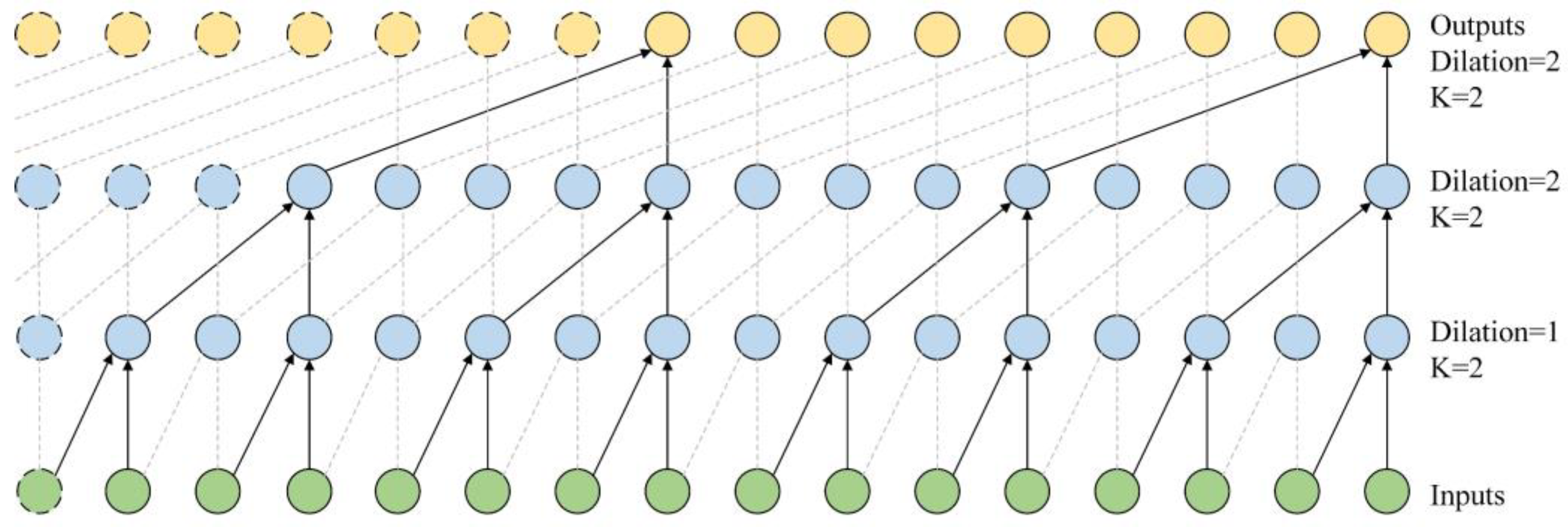
2.3.1. Causal Dilated Convolutional

Causal convolution can be understood as the one-way transmission of temporal data. Unlike traditional convolutional neural networks, in causal convolution, future data cannot affect the past and only performs convolution operations at the current and previous time steps. Hence, it is called causal convolution [47].

As shown in Figure 2, interval sampling is allowed for the input during convolution based on causal convolution. If d = 1, it means sampling each data point; if d = 2, it means sampling every two data points. Similarly, convolutional networks can obtain larger receptive fields even in fewer convolutional layers. Equation (7) is the mathematical expression of causal dilation convolution [43]:

$${\mathrm{y}}_{\mathrm{h},\mathrm{t}}={\displaystyle \sum _{\mathrm{i}=0}^{\mathrm{k}}{\mathrm{f}}_{\mathrm{i}}}\times {\mathrm{y}}_{\mathrm{h}-1}{}_{,\mathrm{t}-2\mathrm{i}\mathrm{d}}$$

(7)

In the equation, ${\mathrm{y}}_{\mathrm{h},\mathrm{t}}$ represents the sequence value of layer h in the network at time t, fi represents the filter, k represents the size of the convolutional kernel, and d represents the convolutional expansion rate.

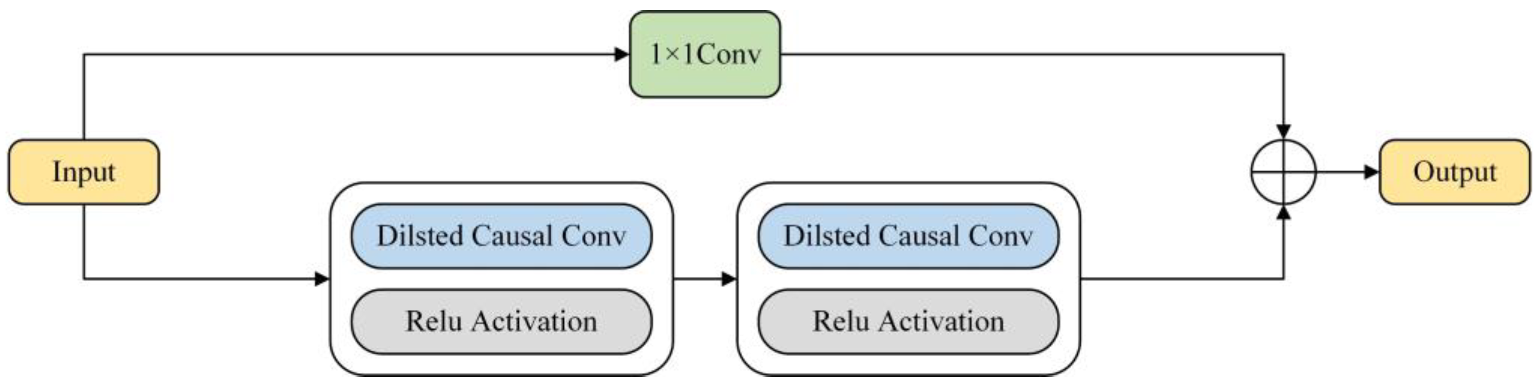
2.3.2. Residual Block

The residual module is a valuable technique for training deep networks because it allows information to be sent between layers, which helps to prevent gradients from disappearing or bursting during deep network training [48,49]. As seen in Figure 3, this article builds a residual block in place of the convolutional layer. Two layers of nonlinear mapping and convolution make up a residual block.

2.4. BiLSTM

LSTM is an improved recurrent neural network that introduces an internal mechanism called a “gate” that can regulate the information flow by learning important information and forgetting secondary information, thereby better handling long-term dependency relationships in sequences. Unlike the standard LSTM, BiLSTM runs two independent LSTM networks simultaneously, one processing input sequences from the front and the other processing input sequences from the back, as shown in Figure 4. This enables the network to capture information before and after each time step, including past and future information.

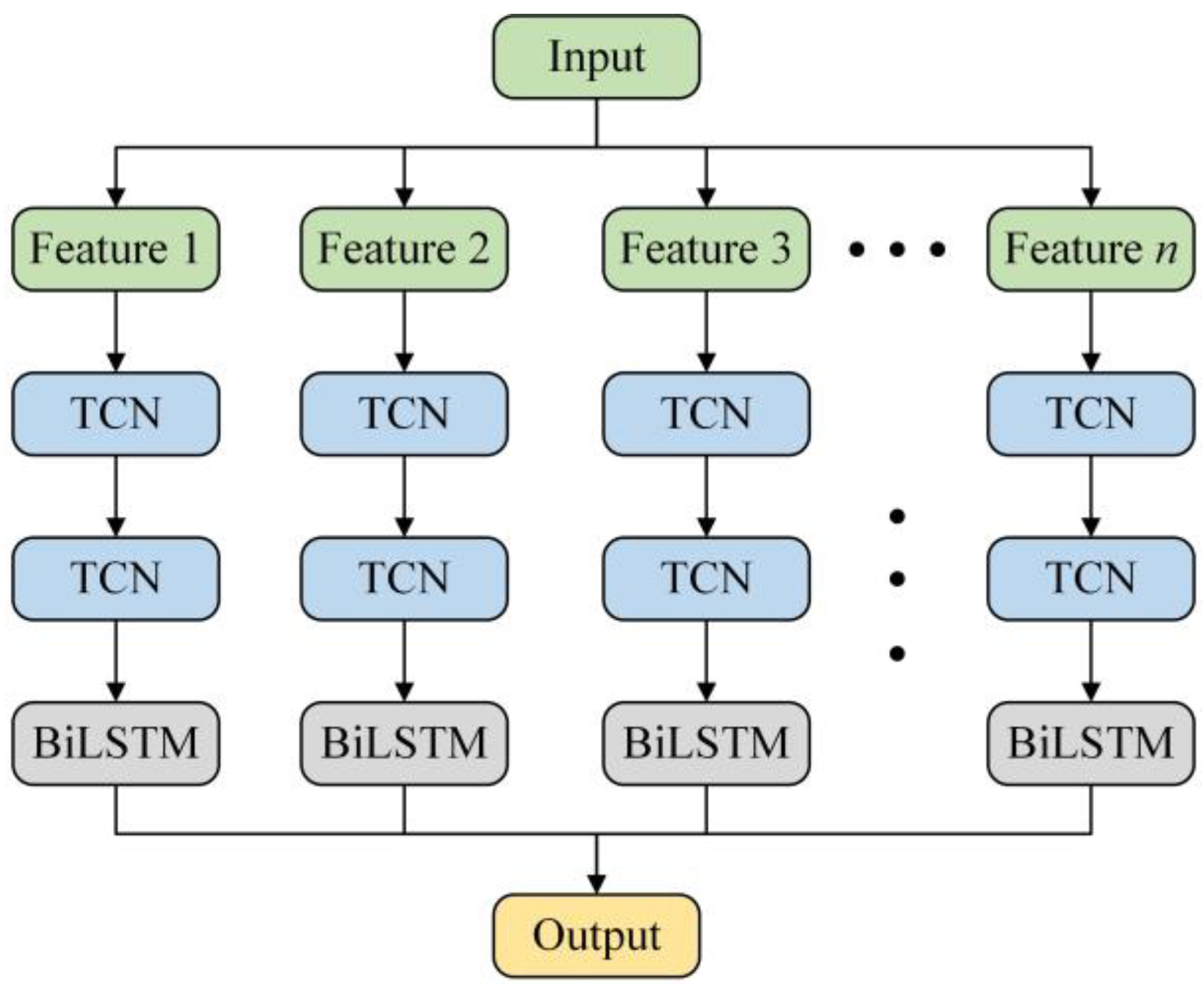
2.5. TCN–BiLSTM

Due to its use of a dilated causal convolution structure, TCN has excellent feature extraction capabilities. Therefore, TCN can fuse original features to obtain higher dimensional abstract features, thereby strengthening the mining of feature information. The BiLSTM network has strong temporal prediction ability. By combining TCN and BiLSTM networks, TCN features are extracted and input into the BiLSTM network, which improves the computational performance of BiLSTM network memory units and makes the prediction model more effective in learning the complex interaction relationships of time series. Therefore, this article constructs a TCN–BiLSTM prediction model, and Figure 5 shows the structure of the combined model.

2.6. Evaluation Index

This article chooses the widely used techniques in landslide displacement prediction, such as the root mean square error (RMSE), coefficient of determination (R²), and mean absolute percentage error (MAPE), to assess the model’s performance in terms of accuracy and applicability. The following is the calculation formula for measurement indicators:

$$\mathrm{R}\mathrm{M}\mathrm{M}\mathrm{S}\mathrm{E}=\sqrt{\frac{1}{\mathrm{n}}{{\displaystyle \sum _{\mathrm{k}=1}^{\mathrm{n}}\left({\widehat{\mathrm{y}}}_{\mathrm{k}}-{\mathrm{y}}_{\mathrm{k}}\right)}}^2}$$

(8)

$$\mathrm{M}\mathrm{A}\mathrm{P}\mathrm{E}=\frac{1}{\mathrm{n}}{\displaystyle \sum _{\mathrm{k}=1}^{\mathrm{n}}\left|\frac{{\widehat{\mathrm{y}}}_{\mathrm{k}}-{\mathrm{y}}_{\mathrm{k}}}{{\mathrm{y}}_{\mathrm{k}}}\right|}\times 100\%$$

(9)

$${\mathrm{R}}^2=1-\frac{{\displaystyle \sum _{\mathrm{k}=1}^{\mathrm{n}}{\left({\widehat{\mathrm{y}}}_{\mathrm{k}}-{\mathrm{y}}_{\mathrm{k}}\right)}^2}}{{\displaystyle \sum _{\mathrm{k}=1}^{\mathrm{n}}{\left({\overline{\mathrm{y}}}_{\mathrm{k}}-{\mathrm{y}}_{\mathrm{k}}\right)}^2}}$$

(10)

In the formula, ${\mathrm{y}}_{\mathrm{k}}$ is the kth true value sample, ${\widehat{\mathrm{y}}}_{\mathrm{k}}$ is the kth predicted value sample, and ${\overline{\mathrm{y}}}_{\mathrm{k}}$ is the arithmetic mean of all true values. Based on the calculation results of RMSE, MAPE, and R², the evaluation is conducted, and the calculation results of all three belong to the range of 0 to 1.

3. Overview of Study Area

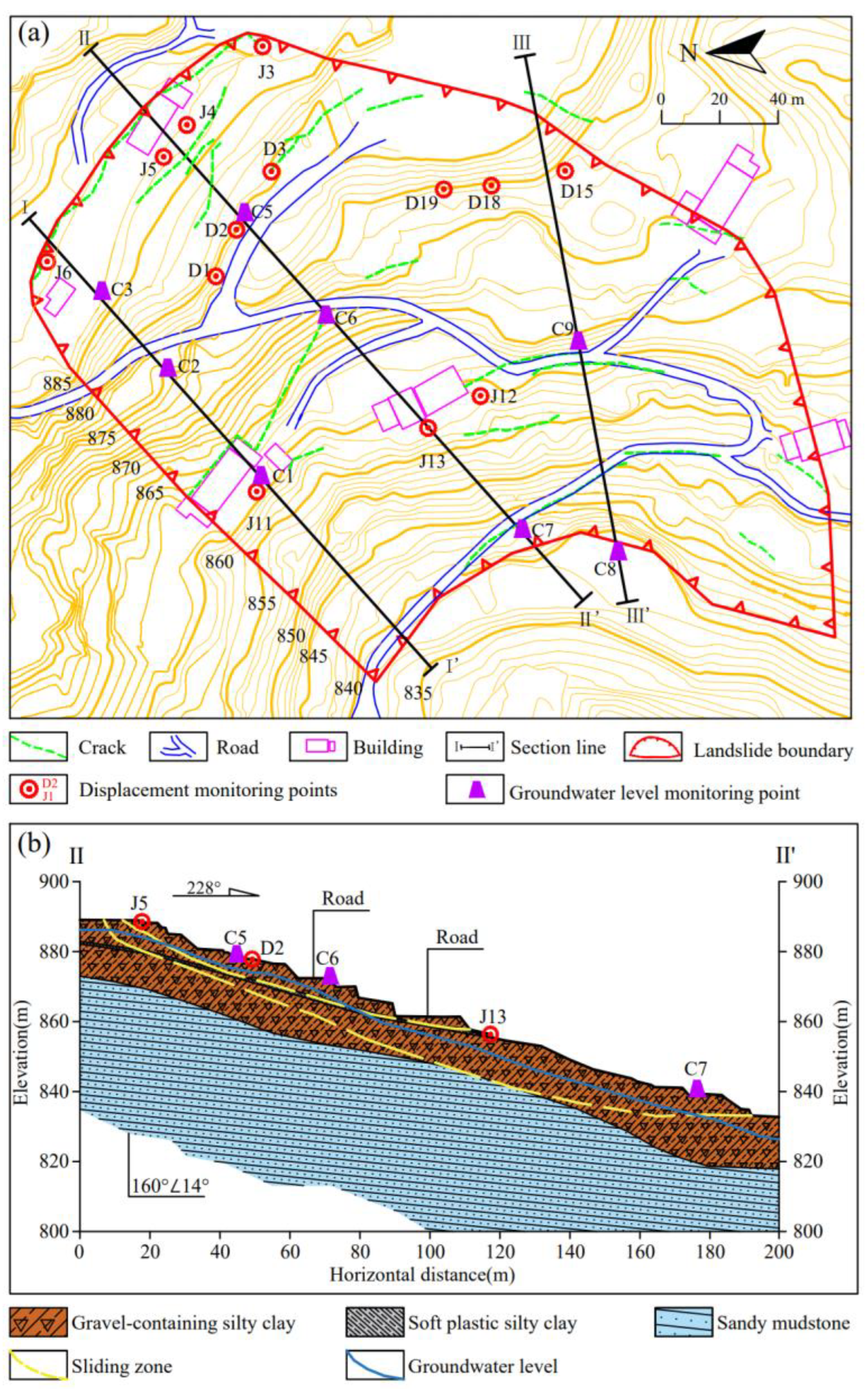
3.1. General Description

The Wanjiawan landslide is located in Anping Village, Xinglong Town, northern Tongjiang County, Sichuan Province. It is situated in Tongjiang County’s northern region, on the west side of the Datongjiang River, and on the east side of the Xiaotongjiang River. The terrain fluctuates greatly, with an overall trend of northeastern high and southwesterly low. The slope direction is about 228°, and the terrain slope is generally 10–20°. The left side of the landslide trailing edge is adjacent to the engineering site leveling area, and the foot of the landslide slope is located in the living camp, as shown in Figure 6.

The overall elevation of the landslide is between 840 m and 890 m, and the width of the entire landslide area is about 222 m. The overall plane shape is in a “circular chair” shape. About 275 m is the landslide’s longitudinal length, with an area of about 3.84 × 104 m². Silty clay containing broken stones makes up most of the sliding soil, and the gravel is mostly composed of sandstone blocks. The landslide volume is around 38.4 × 104 m³, and the landslide mass has an average thickness of roughly 10 m. The sliding zone is a soft plastic silty clay with a small amount of breccia during the period, which has poor water permeability and can form a relatively impermeable layer. The sliding bed is an underlying bedrock, mainly composed of strongly to moderately weathered carbonaceous sandy mudstone and sandstone.

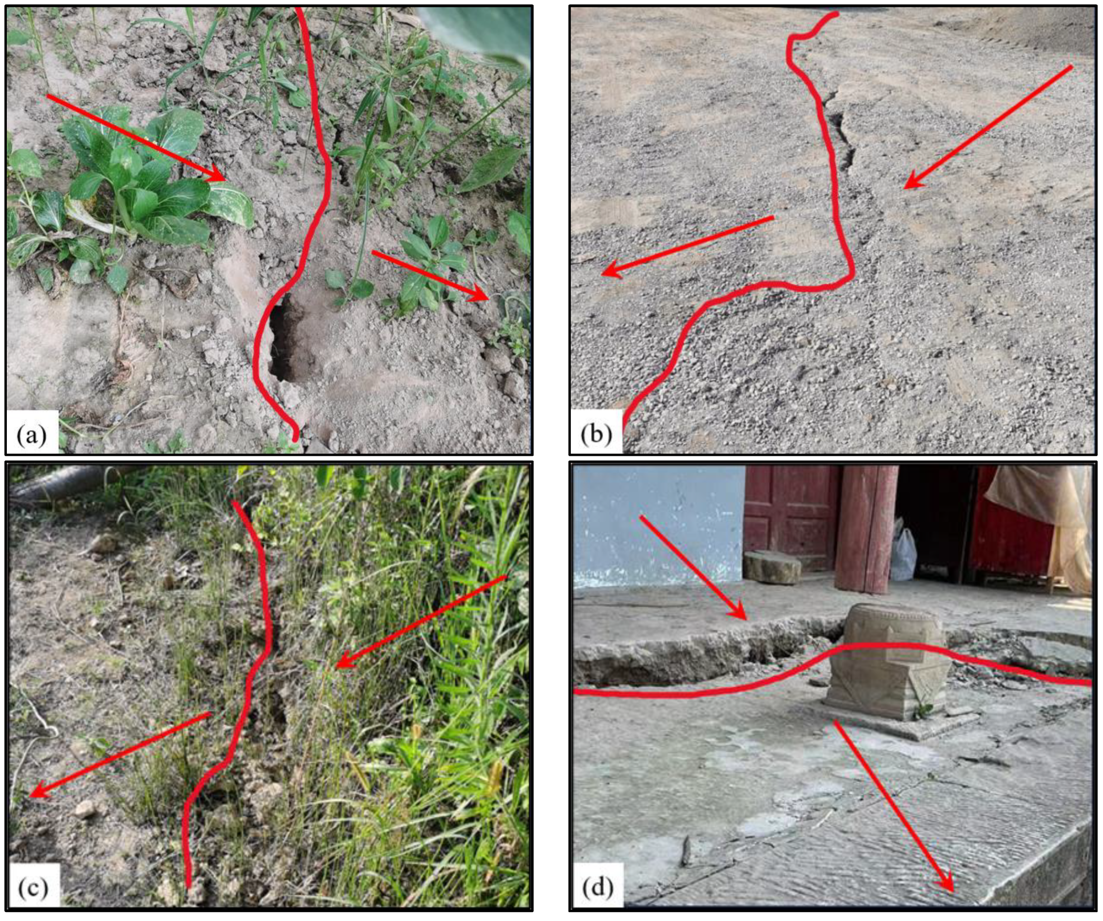
3.2. Macroscopic Deformation Characteristics

The Wanjiawan landslide is a shallow-soil landslide and a medium-sized landslide according to its scale. Due to the exposure of the surface soil layers and the combined effect of long-term rainfall, landslide disasters ultimately occurred. On 7 July 2022, a crack appeared in the upper residential area on the north side of the well pad (Figure 7a), with a maximum crack width of 20 mm and a maximum crack length of 500 mm. From 19 to 27 July 2022, excavation construction was carried out in the slope toe area, during which two rainfall events occurred. The existing cracks on the site expanded, and new cracks appeared in the flat area of the trailing edge engineering site (Figure 7b). Starting on 4 August 2022, displacement monitoring points and groundwater level monitoring points were set up in the landslide area. During the monitoring period, the existing cracks continued to intensify, and new cracks continued to emerge (Figure 7c). From 7 to 28 August 2022, except for the central leveling area of the landslide, the displacement and deformation were relatively stable, with overall small changes, while the deformation in the filling area was relatively large. After two days of continuous rainfall on 30–31 August 2022, the overall deformation of the surface subsidence cracks (Figure 7d) that occurred in the residential area significantly intensified. Based on comprehensive analysis, the landslide has been in the stage of creep deformation and has a tendency to intensify after rainfall.

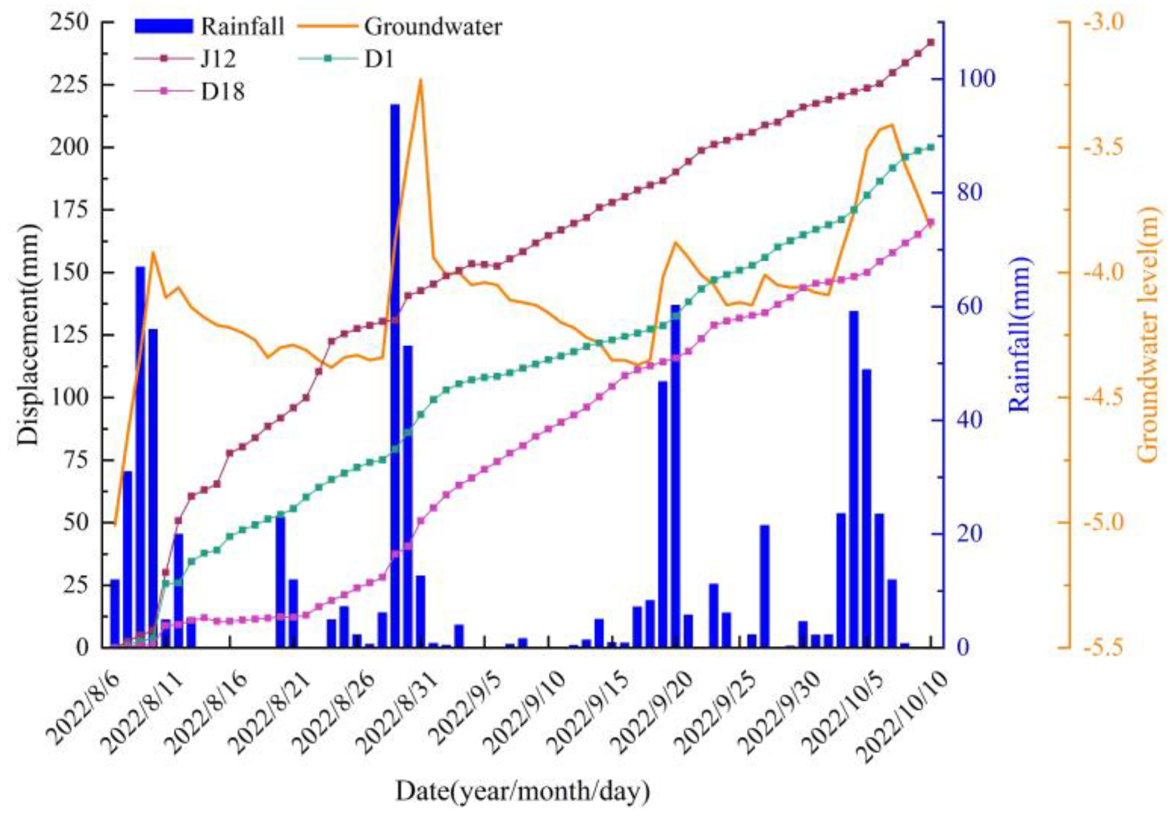
3.3. Analysis of Monitoring Data and Triggering Factors

The factors affecting landslides are often very complex and can be divided into internal factors and external factors according to their sources [50,51,52]. Adverse environmental geological conditions, including slope landforms, thick and loose soil layers, highly weathered lithology, and large-scale free surfaces formed via engineering excavation, are the main internal factors for the occurrence and development of landslides [53]. Under the influence of internal factors, the time displacement relationship curve of the landslide presents an approximate monotonic function, which reflects the trend term of the overall cumulative displacement of the landslide. External factors are different from static factors, and they are mainly dynamic environmental factors outside the landslide, including natural rainfall, groundwater level, wind load, environmental temperature and humidity, etc. Under the influence of external factors, the time displacement relationship curve of the landslide shows a certain regularity of fluctuations.

This project adopts various monitoring methods, and the monitoring data obtained mainly includes rainfall, groundwater level, surface displacement, and deep soil displacement. The above data are all sourced from on-site engineering monitoring reports. After processing and analyzing the data from all monitoring points, the surface displacement monitoring points D1, D18, and J12 located in the middle and lower parts of the landslide showed obvious displacement development trends throughout the entire monitoring cycle. The above three surface displacement monitoring data and the groundwater level monitoring point data located in the middle of the landslide were selected for research. All the monitoring data consisted of 65 periods (from 7 August 2022 to 10 October 2022), as shown in Figure 8.

The monitoring period was during the period of frequent rainfall in the summer, and the groundwater level fluctuated frequently. Two rainstorm events occurred at the beginning and end of August, leading to a sharp rise in the groundwater level, during which the cumulative displacement of each monitoring point increased significantly. During non-rainfall periods, the groundwater level showed a slow downward trend, and the cumulative displacement growth rate slowed down. The two rainstorms in August broke the original stable state of the Wanjiawan slope, and the overall safety reserve of the slope was greatly reduced. Under continuous rainfall in September and October, the cumulative displacement growth trend became larger, and the cumulative displacement increased significantly after the groundwater level rose. During the monitoring cycle, almost all displacement acceleration stages occurred after rainfall events and during groundwater level fluctuations, indicating that changes in the groundwater level and rainfall have a significant impact on landslide deformation. Under the action of rainfall, rainwater seeped down along surface cracks to the relatively impermeable sliding zone interface, and the soft, plastic, powdery clay at the bottom was soaked and softened, resulting in a continuous decrease in the physical and mechanical strength of the sliding zone. At the same time, as the soil’s moisture content increased, the sliding mass’s gravity increased. When the sliding force exceeds the anti-sliding force, soil sliding will occur. Therefore, the acceleration stage of landslide displacement often occurs after rainfall events. As rainfall events continue, groundwater is replenished by atmospheric rainfall, leading to a sharp rise in the water level. The stress and seepage fields inside the slope undergo significant changes in a short period, thereby accelerating landslide events. Therefore, the fluctuation of groundwater levels also leads to the acceleration of landslides.

4. Results

4.1. Data Decomposition

By processing and analyzing all monitoring data, the D1 monitoring point data located in the central area of the landslide showed a clear displacement trend. The integrity of the monitoring data at this point was good, so this article uses this displacement sequence to establish a prediction model for the Wanjiawan landslide. We selected 52 monitoring data sets as training samples from 7 August 2022, to 27 September 2022. The test samples were the following 13 data sets from 28 September 2022 to 10 October 2022. This work developed the ICEEMDAN algorithm in the MATLAB 2022a environment and utilized it to deconstruct the chosen displacement sequence samples, as shown in Equations (3)–(6) above. The parameter settings for this process are as follows: 200 iterations were the maximum, and the standard deviation ratio was 0.15.

The decomposed data are shown in Figure 9. The original displacement sequence sample was divided into four sets of displacement sequence components, with component IMF1 having the highest fluctuation frequency, followed by elements IMF2 and IMF3, and residual component R being relatively smooth with almost no fluctuation. Therefore, the residual component R was considered the trend term displacement, and the sum of components IMF1–IMF3 with significant fluctuations was regarded as the fluctuation term displacement. The combined data are shown in Figure 10.

4.2. Determining Influencing Factors

The reasonable selection of influencing factors determines the upper limit of the accuracy of the prediction model [54,55,56]. Du et al. [57] have shown that the past state of landslides can, to some extent, affect the development trend of landslides. Therefore, this article takes displacement monitoring values as one of the influencing factors of landslides. Rainfall and the reservoir water level are often considered the main factors affecting landslide displacement when studying riverbank slopes [58,59]. The study area of this article is located between the Datong River and the Xiaotong River, and the landslide area is far from the river surface. Therefore, the impact of the reservoir water level on the landslide was not considered. Based on existing engineering monitoring data and careful consideration, rainfall, groundwater level, and historical displacement are the main influencing factors of the Wanjiawan landslide.

Figure 11 shows the relationship between the groundwater level, daily rainfall, and fluctuation term displacement. From the graph, it can be observed that, during periods of frequent rainfall, the displacement of the fluctuation term in the landslide area changes significantly. In weather environments without or with light rain, the displacement of the fluctuation term changes relatively smoothly. Considering that historical rainfall has a significant impact on the future state of landslides, this article takes the cumulative rainfall of the same day, the previous day, and two days as the critical factor affecting landslide displacement (Input 4–6). Furthermore, there was a positive correlation between the changes in the groundwater level in the landslide area and rainfall, and the displacement of the fluctuation term showed a rapid increase when the groundwater level rose. When the groundwater level changed slightly or remained within a certain range, the displacement of the fluctuation term changed less. And the displacement of the fluctuation term often occurred after the groundwater level rose, and the impact of changes in the groundwater level on the displacement of the fluctuation term had a lag effect. Therefore, this article takes the elevation value of the groundwater level on that day, the changes in groundwater level during and after the previous day, and the decrease in groundwater level changes compared to the previous day (Inputs 7–10) as the key influencing factors for the displacement of the fluctuation term. Finally, this article takes the displacement of the previous day, the displacement of the previous two days, and the cumulative displacement of the previous day as the influencing parameters of the fluctuation term displacement (Inputs 1–3).

Based on the above analysis results, this article preliminarily selects ten potential candidate factors, as shown in

Table 1. Candidate factors.

Category	Candidate Triggering Factors
Displacement	Input 1: Displacement over the past one day
	Input 2: Displacement over the past two days
	Input 3: Cumulative displacement of the previous day
Precipitation	Input 4: Cumulative rainfall of the day
	Input 5: Cumulative rainfall within two days
	Input 6: Cumulative rainfall of the previous day
Groundwater level	Input 7: Daily groundwater level elevation
	Input 8: Change in groundwater level elevation in the past day
	Input 9: Change in groundwater level elevation today
	Input 10: Decrease in groundwater level changes compared to the previous day

. Figure 12 shows the GRG and MIC values between various factors. The gray relational grade analysis results indicate that rainfall and the groundwater level had a relatively large impact on the displacement of the fluctuation term. In contrast, historical displacement factors had a relatively small effect on the displacement of the fluctuation term. The results of the maximal information coefficient analysis indicate that the displacement over the past day, the daily groundwater level elevation, and the decrease in groundwater level changes compared to the previous day had a low correlation with the displacement of the fluctuation term. The other candidate factor terms correlated well with the displacement of the fluctuation term; among them, the cumulative displacement of the previous day was highly correlated with the displacement of the fluctuation term. To ensure the accuracy of the prediction results, this article selects candidate factors that meet the conditions of a GRG value greater than 0.80 and an MIC value greater than 0.25 as the main influencing factors of the prediction model. Therefore, this article excludes three candidate factors, Inputs 1, 7, and 10, and identifies the remaining seven as critical factors affecting the displacement of the landslide fluctuation term.

4.3. Displacement Prediction

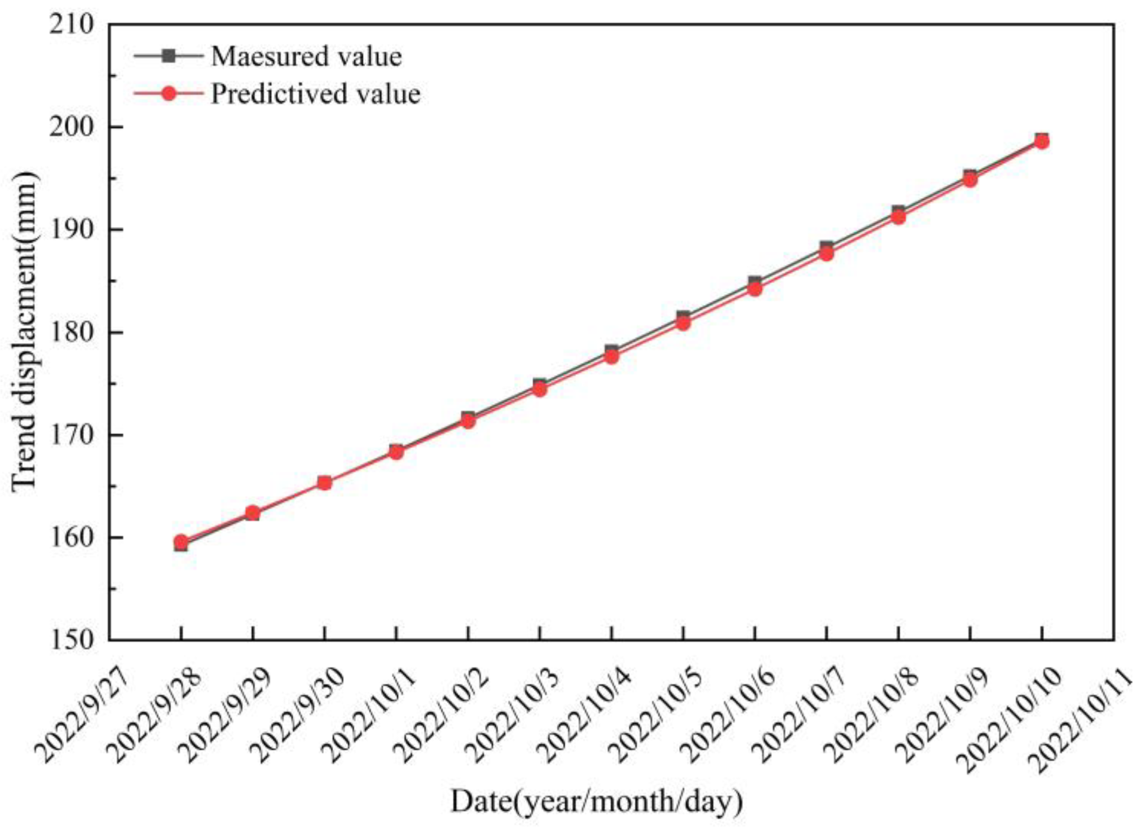
4.3.1. Trend Item Displacement Prediction

The trend term displacement was fitted using polynomial regression equations. To ensure the prediction accuracy of the data as much as possible and avoid overfitting with higher-order polynomials, in this article, multiple experimental analyses were conducted, and it was finally determined to use a cubic polynomial to fit the data. The fitted formula is as follows, with a goodness of fit R² of 0.999, indicating an excellent fitting effect.

$$\mathrm{y}=0.000678115{\mathrm{x}}^3-0.07863{\mathrm{x}}^2+5.41786\mathrm{x}-7.59532$$

(11)

In the equation, $\mathrm{y}$ represents the displacement of the trend term, and $\mathrm{x}$ represents time.

The above equation served as the prediction formula for the trend term in the prediction model, and Figure 13 displays the displacement prediction results of the trend term. The MAPE was 0.002, the RMSE was 0.425, and the R² was 0.999. The calculation results of the evaluation indicators show that using the cubic polynomial fitting method for trend displacement prediction can achieve good prediction results.

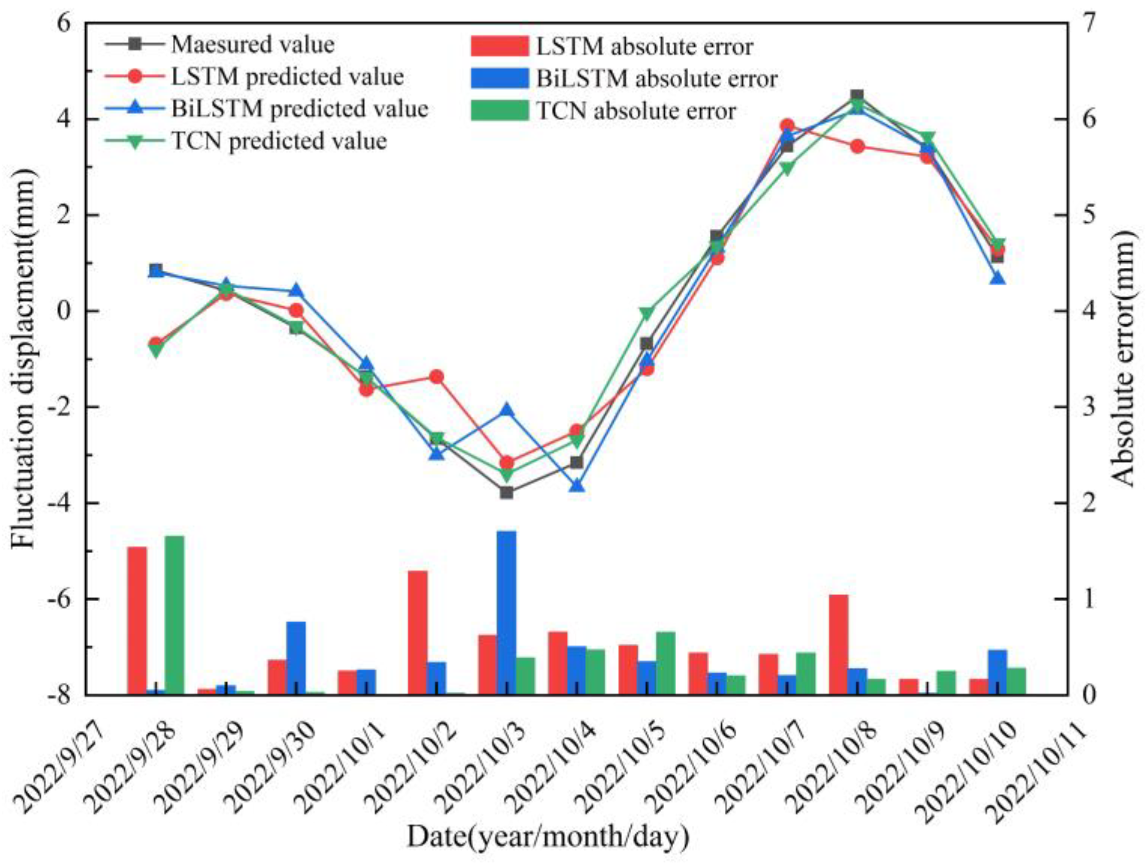
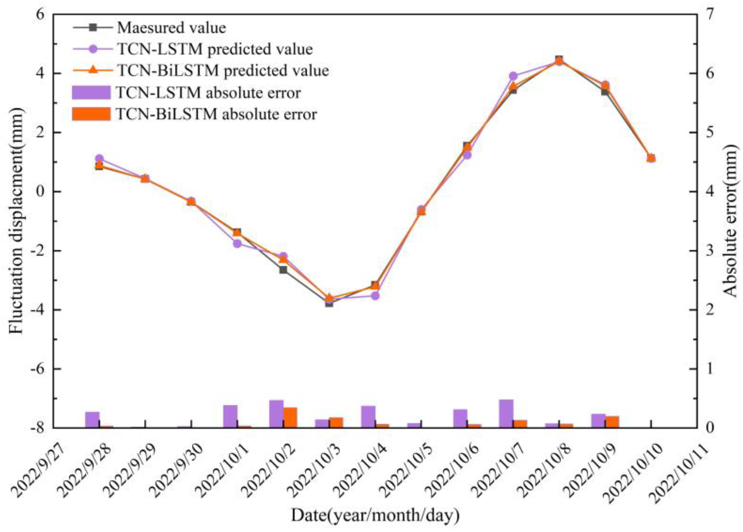
4.3.2. Prediction of Fluctuation Term Displacement

In the TCN model, the expansion factor was set to 4, the convolution kernel size was 3, and the number of hidden layers was set to 4. The hidden layer neurons of the LSTM and BiLSTM models were taken as 64. During training, the input features were the seven most relevant features after correlation filtering, and the first five sets of historical data were used as input items for the model to predict the future two sets of data. The model adopted a Bayesian optimization algorithm for hyperparameter optimization. The combined model also followed the parameter settings of a single model.

Figure 14 displays the prediction results of different neural networks. The LSTM neural network had the worst prediction results for fluctuation term displacement, followed by the TCN neural network and the BiLSTM neural network. The prediction error calculated based on the prediction results is shown in

Table 2. Prediction errors of different neural network models.

Evaluating Indicator	LSTM	BiLSTM	TCN	TCN–LSTM	TCN–BiLSTM
RMSE (mm)	0.725	0.586	0.551	0.274	0.129
MAPE (%)	0.433	0.354	0.305	0.120	0.033
R2	0.915	0.945	0.951	0.988	0.997

. The specific analysis was as follows:

• Due to the limited landslide monitoring data provided in the engineering project, the generalization performance of the trained LSTM model was poor, resulting in an R² of 0.915 and unsatisfactory prediction performance.
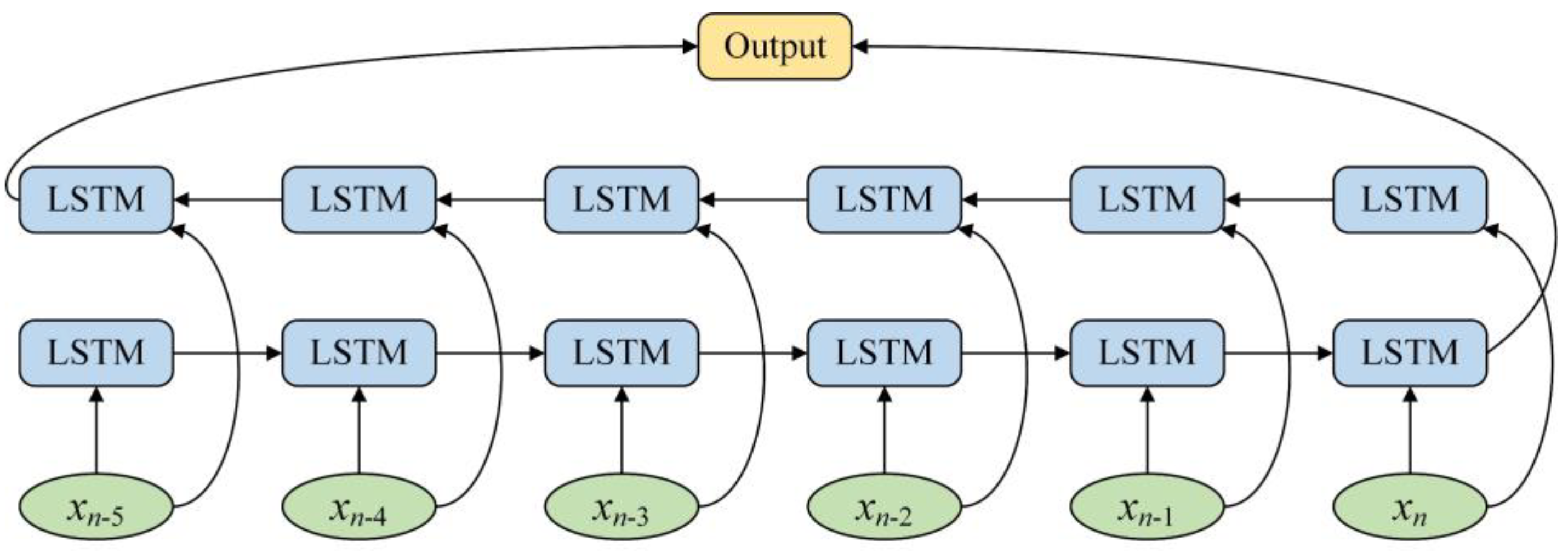
• Due to their unique bidirectional processing structure, BiLSTM neural networks typically provide richer feature representations, which means they can better capture patterns and relationships in input sequences. From the overall error distribution, the prediction error of BiLSTM was slightly lower than LSTM’s. The final calculation result of LSTM neural network R² was 0.945, and the prediction effect was better than that of LSTM.
• The TCN evolved from convolutional neural networks requires fewer parameters than LSTM, making it easier to train and adjust. Therefore, TCN neural networks can achieve more accurate displacement prediction even with limited training data support. The final TCN neural network R² calculation result was 0.945, and the prediction effect was better than that of LSTM.

Overall, the above three types of neural networks achieved good predictive performance in the monotonic increase or decrease stage of the fluctuation term displacement curve. Still, there would be significant errors at the turning points of the fluctuation term displacement curve, which cannot achieve the goal of accurate prediction.

The combination of a single neural network to predict fluctuation term displacement is shown in Figure 15. From the perspective of overall prediction error, the combined two neural network models improved the problem of inaccurate prediction at the turning point of the fluctuation term displacement curve, and the overall prediction accuracy of the model was higher. Among them, TCN–BiLSTM achieved better prediction performance than TCN–LSTM. The specific analysis was as follows.

TCN has a causal dilated convolutional structure and outstanding feature extraction ability. It can fuse original features to obtain high-dimensional abstract features, enhancing the mining of feature information. LSTM and BiLSTM time series networks have strong temporal prediction capabilities, which can better capture patterns and relationships in input sequences. LSTM-type networks can be combined with TCN networks in fluctuation term displacement prediction. By extracting feature variables through TCN and inputting them into the time series network, the processing efficiency of memory units in the time series network is greatly improved. Therefore, the combined prediction model is more effective in learning the complex interaction relationships of the time series.

From the absolute error distribution histogram, the overall error distribution of TCN–BiLSTM was lower than TCN-LSTM’s. Through calculations, the prediction error indicators for the displacement prediction of landslide fluctuation terms using two combination networks were obtained. Compared with TCN–LSTM, the combination of TCN and BiLSTM reduced MAPE by an average of 71.955%, resulting in the higher prediction accuracy of the TCN–BiLSTM combined network.

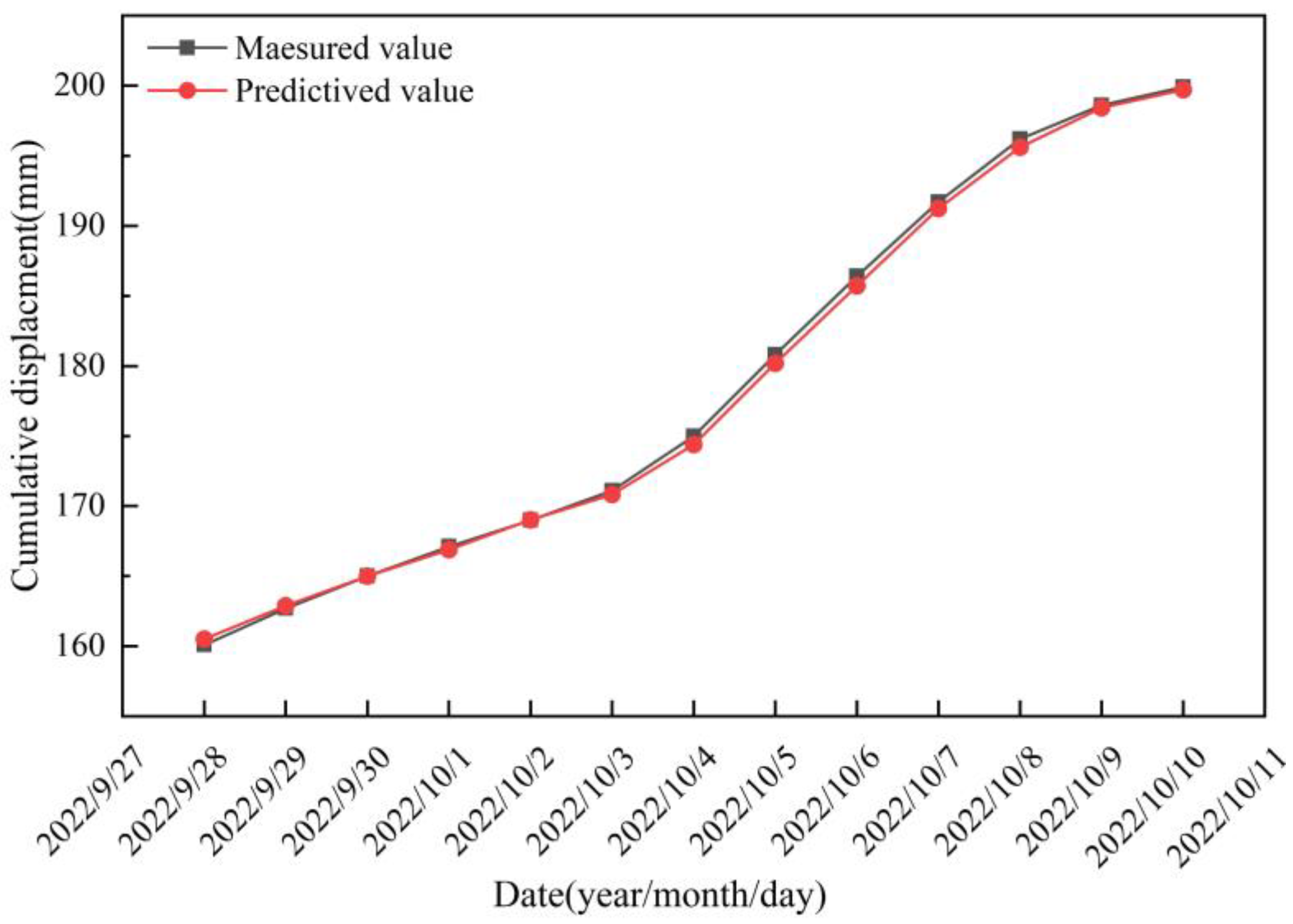
4.3.3. Total Displacement Prediction

As shown in Figure 16, the trend displacement predicted via polynomial fitting was overlaid with the fluctuation displacement predicted using the TCN–BiLSTM combined neural network to obtain the total predicted displacement of the landslide. By comparing the total predicted displacement of the landslide with the actual value, it was found that the predicted total cumulative displacement of the landslide was highly consistent with the actual value. Among the total predicted displacement, MAPE was 0.002, RMSE was 0.406, and R² was 0.999, indicating a good prediction effect.

The experimental results show that the proposed model is more accurate than the other five models in predicting the displacement of landslide fluctuation terms. For nonlinear wave term displacement curves, the accurate prediction of data points at curve turning points is crucial. The model’s feature extraction and learning ability determine the accuracy of displacement predictions. TCN and BiLSTM achieved lower prediction errors in a single neural network than LSTM. This was due to the excellent feature extraction ability of the TCN model, which can deeply mine nonlinear features. The bidirectional LSTM network structure can fully utilize input feature information to obtain richer feature representations for learning. Combining TCN with BiLSTM can achieve the accurate prediction of nonlinear features. The displacement of the fluctuation term of the Wanjiawan landslide is related to rainfall and groundwater level height, and these characteristic changes are often nonlinear during rainy periods. Therefore, constructing a TCN–BiLSTM combination model can more accurately grasp the movement trend of the landslide.

On the other hand, the TCN–BiLSTM combination model has a high level of complexity and requires more computational resources and time for training. Therefore, selecting key input features is particularly important during the training process.

5. Conclusions

This article has focused on the high-precision displacement prediction problem of rainfall-induced landslides, deeply analyzed the relationship between influencing factors and the cumulative displacement of landslides, and combined the advantages of BiLSTM and TCN to propose a rainfall-induced landslide displacement prediction model based on a TCN–BiLSTM combined structural neural network. And this prediction model was applied to the displacement prediction of the Wanjiawan landslide, and its prediction results were compared with the prediction results of the LSTM, TCN, BiLSTM, and TCN–LSTM models. The following conclusions were drawn:

(1)

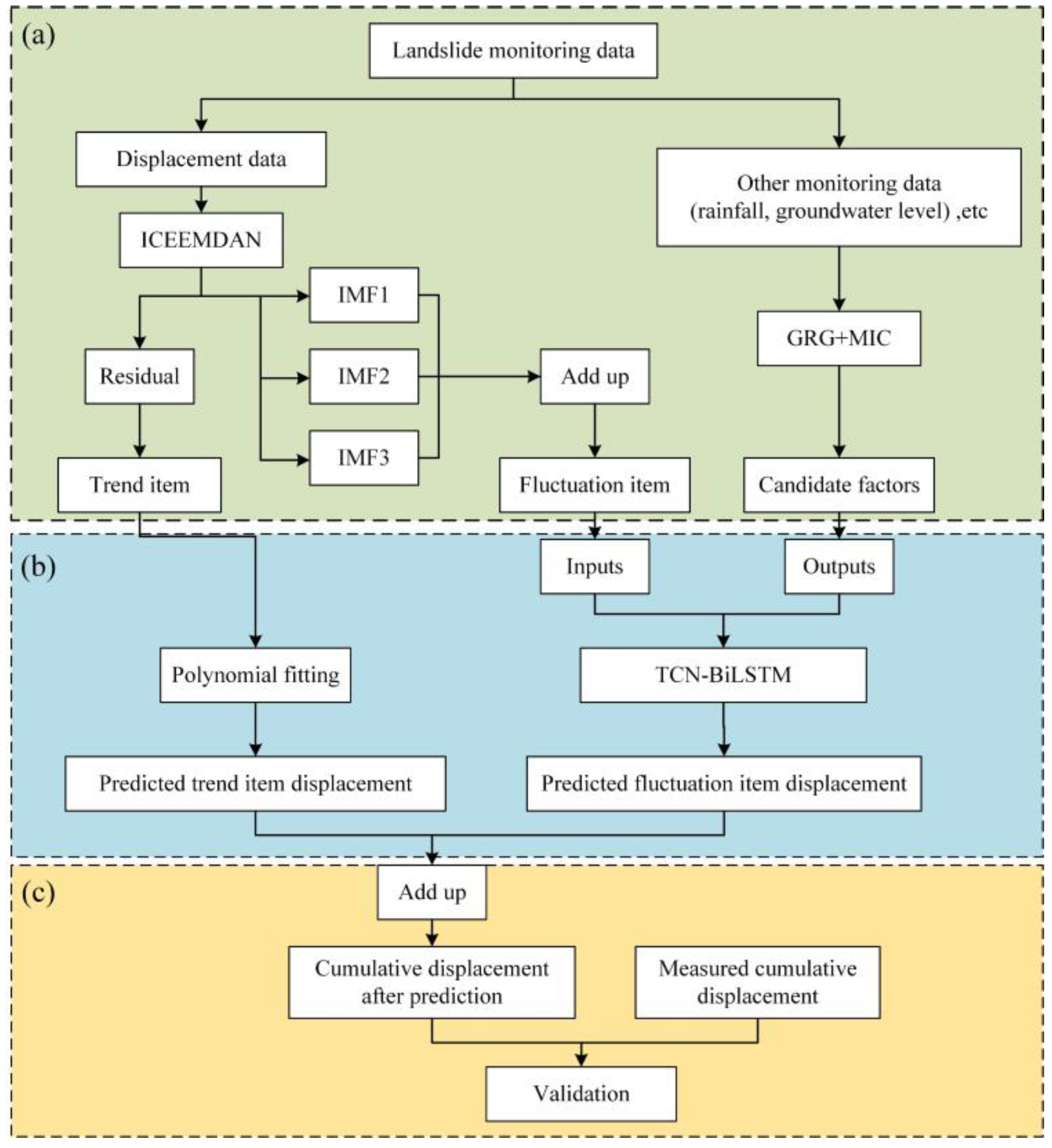
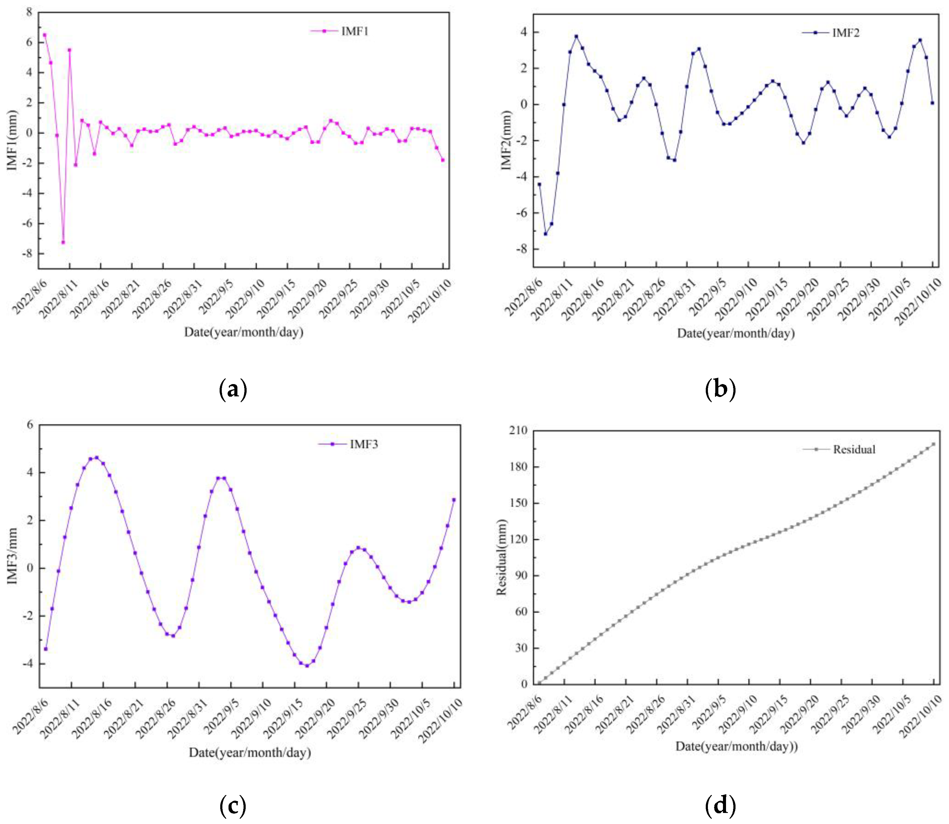
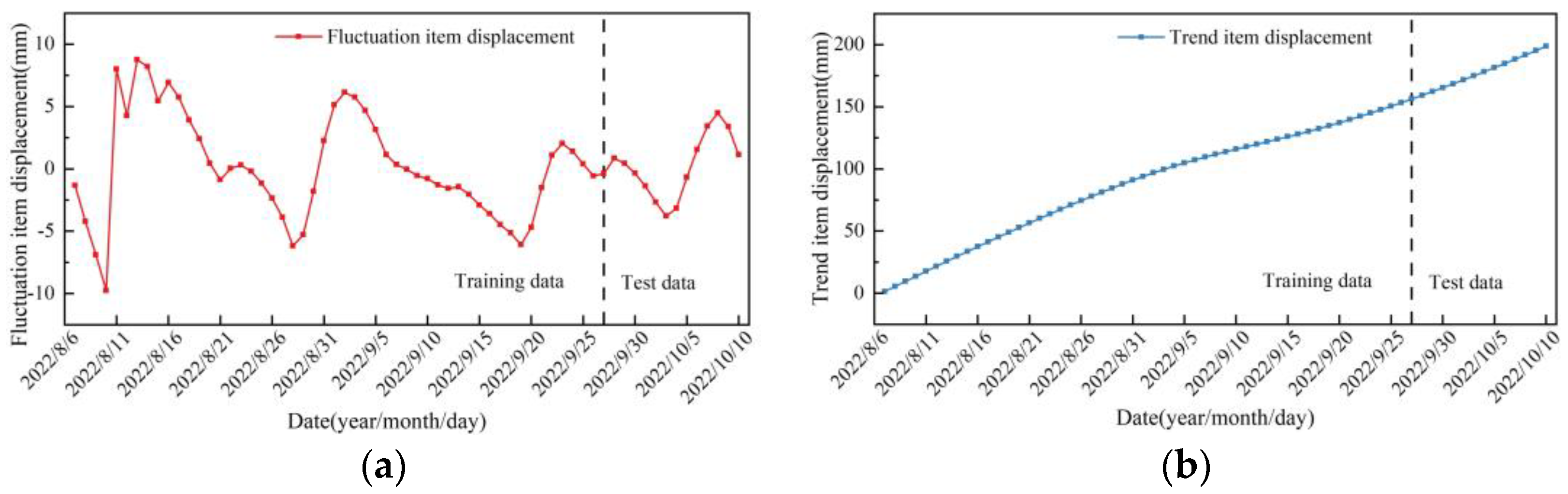
The ICEEMDAN algorithm has strong adaptability to decomposing landslide displacement sequences. By selecting a reasonable signal-to-noise ratio decomposition, the cumulative displacement of landslides can be effectively decomposed into relatively stable, high-frequency fluctuation terms and low-frequency residual terms, and the resulting displacement components have practical physical significance.

(2)

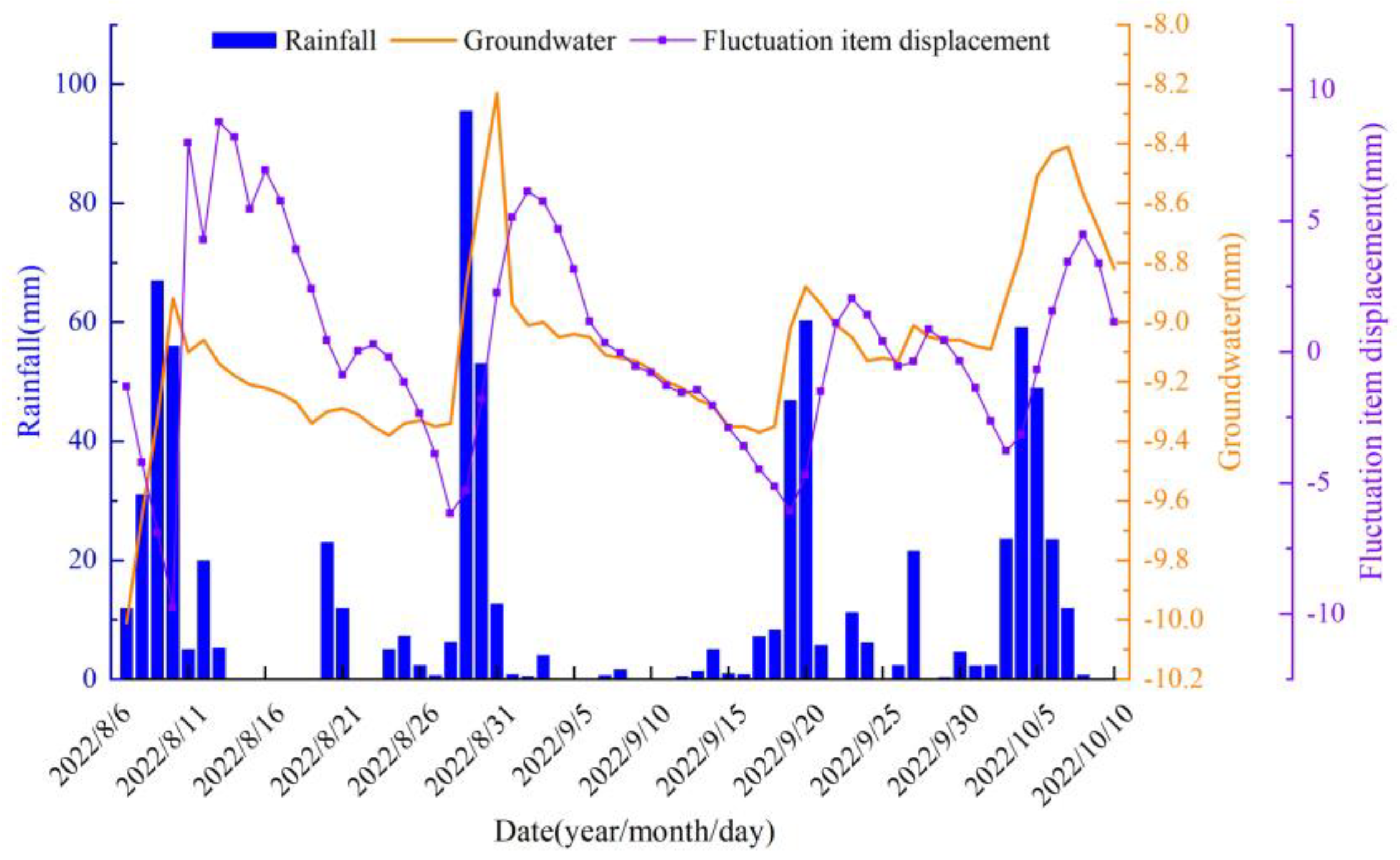
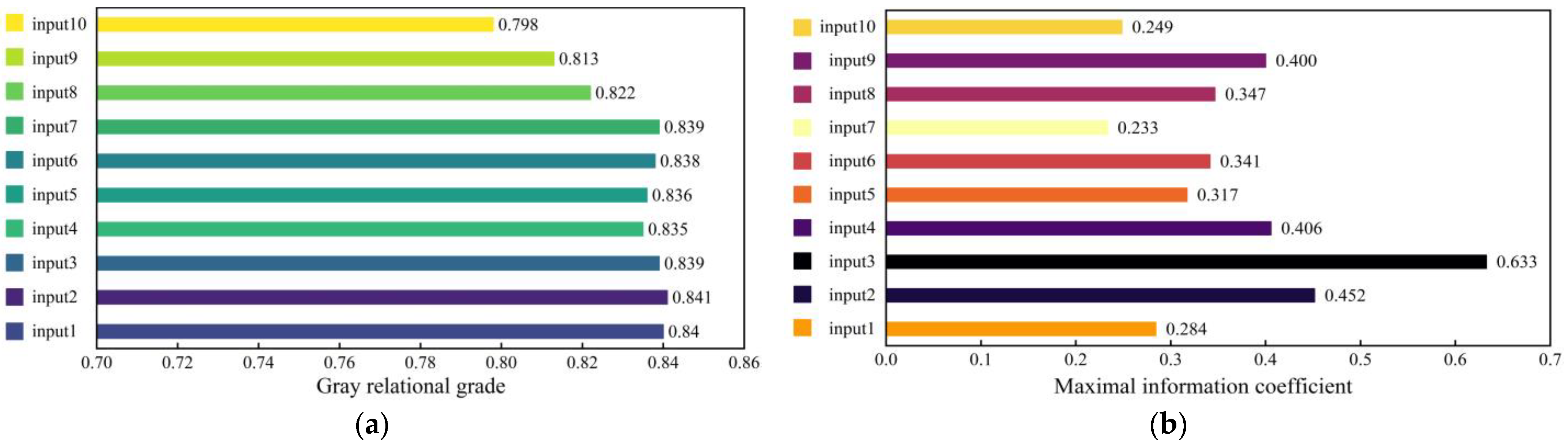
In the selection of characteristic data for predicting landslide displacement fluctuation terms, precipitation, the groundwater level, and the historical displacement of landslides are highly correlated with the displacement components of landslide fluctuation terms. This article used the GRG–MCI combination screening method to process the processed parameter data, and the influencing factors identified were highly correlated with the displacement component of the landslide fluctuation term.

(3)

For landslide trend displacement prediction, using the polynomial fitting method can achieve good prediction results, with a predicted value of R² of 0.999, which indicates high prediction accuracy and can accurately reflect the trend changes of landslide displacement. In predicting the displacement of landslide fluctuation terms, the TCN–BiLSTM combined structural neural network model can accurately capture the fluctuation changes of landslide displacement, with a predicted value of R² of 0.997, which performs better than the conventional LSTM, TCN, BiLSTM, and TCN–LSTM models.

(4)

This article used the ICEEMDAN–TCN–BiLSTM model to predict the displacement of the D1 monitoring point of the Wanjiawan landslide. The various evaluation indicators of the predicted results prove that the model has high applicability for landslide displacement prediction. Based on this, it was inferred that this method can be effectively used to predict displacement at other landslide locations. However, its applicability in predicting the displacement of other types of landslides still needs further verification.

References

- Jing, Y.; Wang, W.; Zou, L.; Wang, R.; Liu, S.; Duan, X. Research on dynamic prediction model of landslide displacement based on particle swarm optimization-variational mode decomposition, nonlinear autoregressive neural network with exogenous inputs and gated recurrent unit. Rock Soil Mech. 2022, 43, 601–612. [Google Scholar]
- Zhang, J.; Yin, K.; Wang, J.; Huang, F. Displacement prediction of baishuihe landslide based on time series and PSO-SVR model. Chin. J. Rock Mech. Eng. 2015, 34, 382–391. [Google Scholar]
- Zhang, J.; Tang, H.; Wen, T.; Ma, J.; Tan, Q.; Xia, D.; Liu, X.; Zhang, Y. A Hybrid Landslide Displacement Prediction Method Based on CEEMD and DTW-ACO-SVR—Cases Studied in the Three Gorges Reservoir Area. Sensors 2020, 20, 4287. [Google Scholar] [CrossRef] [PubMed]
- Li, L.; Wu, Y.; Miao, F.; Xue, Y.; Huang, Y. A hybrid interval displacement forecasting model for reservoir colluvial landslides with step-like deformation characteristics considering dynamic switching of deformation states. Stoch. Environ. Res. Risk Assess. 2021, 35, 1089–1112. [Google Scholar] [CrossRef]
- Haghshenas, S.S.; Haghshenas, S.S.; Geem, Z.W.; Kim, T.-H.; Mikaeil, R.; Pugliese, L.; Troncone, A. Application of harmony search algorithm to slope stability analysis. Land 2021, 10, 1250. [Google Scholar] [CrossRef]
- Shu, B.; He, Y.; Wang, L.; Zhang, Q.; Li, X.; Qu, X.; Huang, G.; Qu, W. Real-time high-precision landslide displacement monitoring based on a GNSS CORS network. Measurement 2023, 217, 113056. [Google Scholar] [CrossRef]
- Iverson, R.M. Landslide triggering by rain infiltration. Water Resour. Res. 2000, 36, 1897–1910. [Google Scholar] [CrossRef]
- Springman, S.M.; Thielen, A.; Kienzler, P.; Friedel, S. A long-term field study for the investigation of rainfall-induced landslides. Geotechnique 2013, 63, 1177–1193. [Google Scholar] [CrossRef]
- Lee, M.L.; Ng, K.Y.; Huang, Y.F.; Li, W.C. Rainfall-induced landslides in Hulu Kelang area, Malaysia. Nat. Hazards 2014, 70, 353–375. [Google Scholar] [CrossRef]
- Collins, B.D.; Znidarcic, D. Stability analyses of rainfall induced landslides. J. Geotech. Geoenviron. Eng. 2004, 130, 362–372. [Google Scholar] [CrossRef]
- Piciullo, L.; Calvello, M.; Cepeda, J.M. Territorial early warning systems for rainfall-induced landslides. Earth-Sci. Rev. 2018, 179, 228–247. [Google Scholar] [CrossRef]
- Jiang, Y.; Liao, L.; Luo, H.; Zhu, X.; Lu, Z. Multi-Scale Response Analysis and Displacement Prediction of Landslides Using Deep Learning with JTFA: A Case Study in the Three Gorges Reservoir, China. Remote Sens. 2023, 15, 3995. [Google Scholar] [CrossRef]
- Van Asch, T.W.; Buma, J.; Van Beek, L. A view on some hydrological triggering systems in landslides. Geomorphology 1999, 30, 25–32. [Google Scholar] [CrossRef]
- Premchitt, J.; Brand, E.; Phillipson, H. Landslides caused by rapid groundwater changes. Geol. Soc. Lond. Eng. Geol. Spec. Publ. 1986, 3, 87–94. [Google Scholar] [CrossRef]
- Liu, Q.; Jian, W.; Nie, W. Rainstorm-induced landslides early warning system in mountainous cities based on groundwater level change fast prediction. Sustain. Cities Soc. 2021, 69, 102817. [Google Scholar] [CrossRef]
- Wang, L.; Wu, C.; Yang, Z.; Wang, L. Deep learning methods for time-dependent reliability analysis of reservoir slopes in spatially variable soils. Comput. Geotech. 2023, 159, 105413. [Google Scholar] [CrossRef]
- Meunier, P.; Hovius, N.; Haines, A.J. Regional patterns of earthquake-triggered landslides and their relation to ground motion. Geophys. Res. Lett. 2007, 34. [Google Scholar] [CrossRef]
- Zhu, S.; Shi, Y.; Lu, M.; Xie, F. Dynamic mechanisms of earthquake-triggered landslides. Sci. China Earth Sci. 2013, 56, 1769–1779. [Google Scholar] [CrossRef]
- Li, C.; Wang, G.; He, J.; Wang, Y. A novel approach to probabilistic seismic landslide hazard mapping using Monte Carlo simulations. Eng. Geol. 2022, 301, 106616. [Google Scholar] [CrossRef]
- Huang, X.; Wang, L.; Ye, R.; Yi, W.; Huang, H.; Guo, F.; Huang, G. Study on deformation characteristics and mechanism of reactivated ancient landslides induced by engineering excavation and rainfall in Three Gorges Reservoir area. Nat. Hazards 2022, 110, 1621–1647. [Google Scholar] [CrossRef]
- Li, Y.; Wang, X.; Mao, H. Influence of human activity on landslide susceptibility development in the Three Gorges area. Nat. Hazards 2020, 104, 2115–2151. [Google Scholar] [CrossRef]
- Hong, B.; Shao, B.; Wang, B.; Zhao, J.; Qian, J.; Guo, J.; Xu, Y.; Li, C.; Zhu, B. Using the meteorological early warning model to improve the prediction accuracy of water damage geological disasters around pipelines in mountainous areas. Sci. Total Environ. 2023, 889, 164334. [Google Scholar] [CrossRef] [PubMed]
- Yang, S.; Jin, A.; Nie, W.; Liu, C.; Li, Y. Research on SSA-LSTM-based slope monitoring and early warning model. Sustainability 2022, 14, 10246. [Google Scholar] [CrossRef]
- Li, L.; Wu, Y.; Miao, F.; Liao, K.; Zhang, L. Displacement prediction of landslides based on variational mode decomposition and GWO-MIC-SVR model. Chin. J. Rock Mech. Eng. 2018, 37, 1395–1406. [Google Scholar]
- Du, J.; Yin, K.; Chai, B. Study of displacement prediction model of landslide based on response analysis of inducing factors. Chin. J. Rock Mech. Eng. 2009, 28, 1783–1789. [Google Scholar]
- Yang, F.; Xu, Q.; Fan, X.; Ye, W. Prediction of landslide displacement time series based on support vector regression machine with artificial bee colony algorithm. J. Eng. Geol. 2019, 27, 880–889. [Google Scholar]
- Liu, Y.; Xu, C.; Huang, B.; Ren, X.; Liu, C.; Hu, B.; Chen, Z. Landslide displacement prediction based on multi-source data fusion and sensitivity states. Eng. Geol. 2020, 271, 105608. [Google Scholar] [CrossRef]
- Zhang, K.; Zhang, K.; Cai, C.; Liu, W.; Xie, J. Displacement prediction of step-like landslides based on feature optimization and VMD-Bi-LSTM: A case study of the Bazimen and Baishuihe landslides in the Three Gorges, China. Bull. Eng. Geol. Environ. 2021, 80, 8481–8502. [Google Scholar] [CrossRef]
- Zhang, J.; Tang, H.; Tannant, D.D.; Lin, C.; Xia, D.; Wang, Y.; Wang, Q. A novel model for landslide displacement prediction based on EDR selection and multi-swarm intelligence optimization algorithm. Sensors 2021, 21, 8352. [Google Scholar] [CrossRef]
- Bommidi, B.S.; Teeparthi, K.; Kosana, V. Hybrid wind speed forecasting using ICEEMDAN and transformer model with novel loss function. Energy 2023, 265, 126383. [Google Scholar] [CrossRef]
- Zou, X.; He, D.; Jin, Z.; Wei, Z.; Miao, J. Intelligent diagnosis method of bearing fault based on ICEEMDAN and Ghost-IRCNN. Proc. Inst. Mech. Eng. Part C J. Mech. Eng. Sci. 2023, 237, 3115–3130. [Google Scholar] [CrossRef]
- Colominas, M.A.; Schlotthauer, G.; Torres, M.E. Improved complete ensemble EMD: A suitable tool for biomedical signal processing. Biomed. Signal Process. Control. 2014, 14, 19–29. [Google Scholar] [CrossRef]
- Zhang, X.; Chen, H.; Wen, Y.; Shi, J.; Xiao, Y. A new rainfall prediction model based on ICEEMDAN-WSD-BiLSTM and ESN. Environ. Sci. Pollut. Res. 2023, 30, 53381–53396. [Google Scholar] [CrossRef] [PubMed]
- Wang, H.; Long, G.; Shao, P.; Lv, Y.; Gan, F.; Liao, J. A DES-BDNN based probabilistic forecasting approach for step-like landslide displacement. J. Clean. Prod. 2023, 394, 136281. [Google Scholar] [CrossRef]
- Meng, Q.; Wang, H.; He, M.; Gu, J.; Qi, J.; Yang, L. Displacement prediction of water-induced landslides using a recurrent deep learning model. Eur. J. Environ. Civ. Eng. 2023, 27, 2460–2474. [Google Scholar] [CrossRef]
- Lin, Z.; Sun, X.; Ji, Y. Landslide displacement prediction based on time series analysis and double-BiLSTM model. Int. J. Environ. Res. Public Health 2022, 19, 2077. [Google Scholar] [CrossRef]
- Xu, S.; Niu, R. Displacement prediction of Baijiabao landslide based on empirical mode decomposition and long short-term memory neural network in Three Gorges area, China. Comput. Geosci. 2018, 111, 87–96. [Google Scholar] [CrossRef]
- Yang, B.; Yin, K.; Lacasse, S.; Liu, Z. Time series analysis and long short-term memory neural network to predict landslide displacement. Landslides 2019, 16, 677–694. [Google Scholar] [CrossRef]
- Zhang, X.; Zhu, C.; He, M.; Dong, M.; Zhang, G.; Zhang, F. Failure mechanism and long short-term memory neural network model for landslide risk prediction. Remote Sens. 2021, 14, 166. [Google Scholar] [CrossRef]
- Zhang, W.; Li, H.; Tang, L.; Gu, X.; Wang, L.; Wang, L. Displacement prediction of Jiuxianping landslide using gated recurrent unit (GRU) networks. Acta Geotech. 2022, 17, 1367–1382. [Google Scholar] [CrossRef]
- Zhang, Y.-g.; Tang, J.; He, Z.-y.; Tan, J.; Li, C. A novel displacement prediction method using gated recurrent unit model with time series analysis in the Erdaohe landslide. Nat. Hazards 2021, 105, 783–813. [Google Scholar] [CrossRef]
- Hewage, P.; Behera, A.; Trovati, M.; Pereira, E.; Ghahremani, M.; Palmieri, F.; Liu, Y. Temporal convolutional neural (TCN) network for an effective weather forecasting using time-series data from the local weather station. Soft Comput. 2020, 24, 16453–16482. [Google Scholar] [CrossRef]
- Fan, J.; Zhang, K.; Huang, Y.; Zhu, Y.; Chen, B. Parallel spatio-temporal attention-based TCN for multivariate time series prediction. Neural Comput. Appl. 2023, 35, 13109–13118. [Google Scholar] [CrossRef]
- Huang, N.E.; Shen, Z.; Long, S.R.; Wu, M.C.; Shih, H.H.; Zheng, Q.; Yen, N.-C.; Tung, C.C.; Liu, H.H. The empirical mode decomposition and the Hilbert spectrum for nonlinear and non-stationary time series analysis. Proc. R. Soc. London. Ser. A Math. Phys. Eng. Sci. 1998, 454, 903–995. [Google Scholar] [CrossRef]
- Lee, K.; Suk, J.; Kim, H.; Jeong, S. Modeling of rainfall-induced landslides using a full-scale flume test. Landslides 2021, 18, 1153–1162. [Google Scholar] [CrossRef]
- Zhou, X.; Wang, J.; Cao, X.; Fan, Y.; Duan, Q. Simulation of future dissolved oxygen distribution in pond culture based on sliding window-temporal convolutional network and trend surface analysis. Aquac. Eng. 2021, 95, 102200. [Google Scholar] [CrossRef]
- Li, W.; Jiang, X. Prediction of air pollutant concentrations based on TCN-BiLSTM-DMAttention with STL decomposition. Sci. Rep. 2023, 13, 4665. [Google Scholar] [CrossRef]
- Xing, M.; Ding, W.; Li, H.; Zhang, T. A power transformer fault prediction method through temporal convolutional network on dissolved gas chromatography data. Secur. Commun. Netw. 2022, 2022, 5357412. [Google Scholar] [CrossRef]
- Zheng, Q.; Zheng, J.; Mei, F.; Gao, A.; Zhang, X.; Xie, Y. TCN-GAT multivariate load forecasting model based on SHAP value selection strategy in integrated energy system. Front. Energy Res. 2023, 11, 1208502. [Google Scholar] [CrossRef]
- Lee, J.-J.; Song, M.-S.; Yun, H.-S.; Yum, S.-G. Dynamic landslide susceptibility analysis that combines rainfall period, accumulated rainfall, and geospatial information. Sci. Rep. 2022, 12, 18429. [Google Scholar] [CrossRef]
- Liu, X.; Lan, H.; Li, L.; Cui, P. An ecological indicator system for shallow landslide analysis. Catena 2022, 214, 106211. [Google Scholar] [CrossRef]
- Tran, T.; Alvioli, M.; Hoang, V. Description of a complex, rainfall-induced landslide within a multi-stage three-dimensional model. Nat. Hazards 2022, 110, 1953–1968. [Google Scholar] [CrossRef]
- Zhou, C.; Yin, K.; Cao, Y.; Intrieri, E.; Ahmed, B.; Catani, F. Displacement prediction of step-like landslide by applying a novel kernel extreme learning machine method. Landslides 2018, 15, 2211–2225. [Google Scholar] [CrossRef]
- Yang, Z.; Gao, W. Applications of machine learning in alloy catalysts: Rational selection and future development of descriptors. Adv. Sci. 2022, 9, 2106043. [Google Scholar] [CrossRef]
- Zhang, W.; Huang, W.; Tan, J.; Huang, D.; Ma, J.; Wu, B. Modeling, optimization and understanding of adsorption process for pollutant removal via machine learning: Recent progress and future perspectives. Chemosphere 2023, 311, 137044. [Google Scholar] [CrossRef]
- Huang, F.; Pan, L.; Fan, X.; Jiang, S.-H.; Huang, J.; Zhou, C. The uncertainty of landslide susceptibility prediction modeling: Suitability of linear conditioning factors. Bull. Eng. Geol. Environ. 2022, 81, 182. [Google Scholar] [CrossRef]
- Du, Y.; Ning, L.; Xie, M.; Bai, Y.; Li, H.; Jia, B. A Prediction Model of Landslide Displacement in Reservoir Area Considering Time Lag Effect. Geomat. Inf. Sci. Wuhan Univ. 2023, 1–12. [Google Scholar] [CrossRef]
- Duan, G.; Su, Y.; Fu, J. Landslide Displacement Prediction Based on Multivariate LSTM Model. Int. J. Environ. Res. Public Health 2023, 20, 1167. [Google Scholar] [CrossRef]
- Junwei, W.; Yiliang, L.; Guangcheng, Z.; Xinli, H.; Baoyin, X.; Dasheng, W. Reservoir Landslide Displacement Prediction Under Rainfall Based on the ILF-FFT Method. Bull. Eng. Geol. Environ. 2023, 82, 179. [Google Scholar] [CrossRef]