

A Prediction Model of Coal Seam Roof Water Abundance Based on PSO-GA-BP Neural Network
 , ,
, ,
Abstract
:1. Introduction
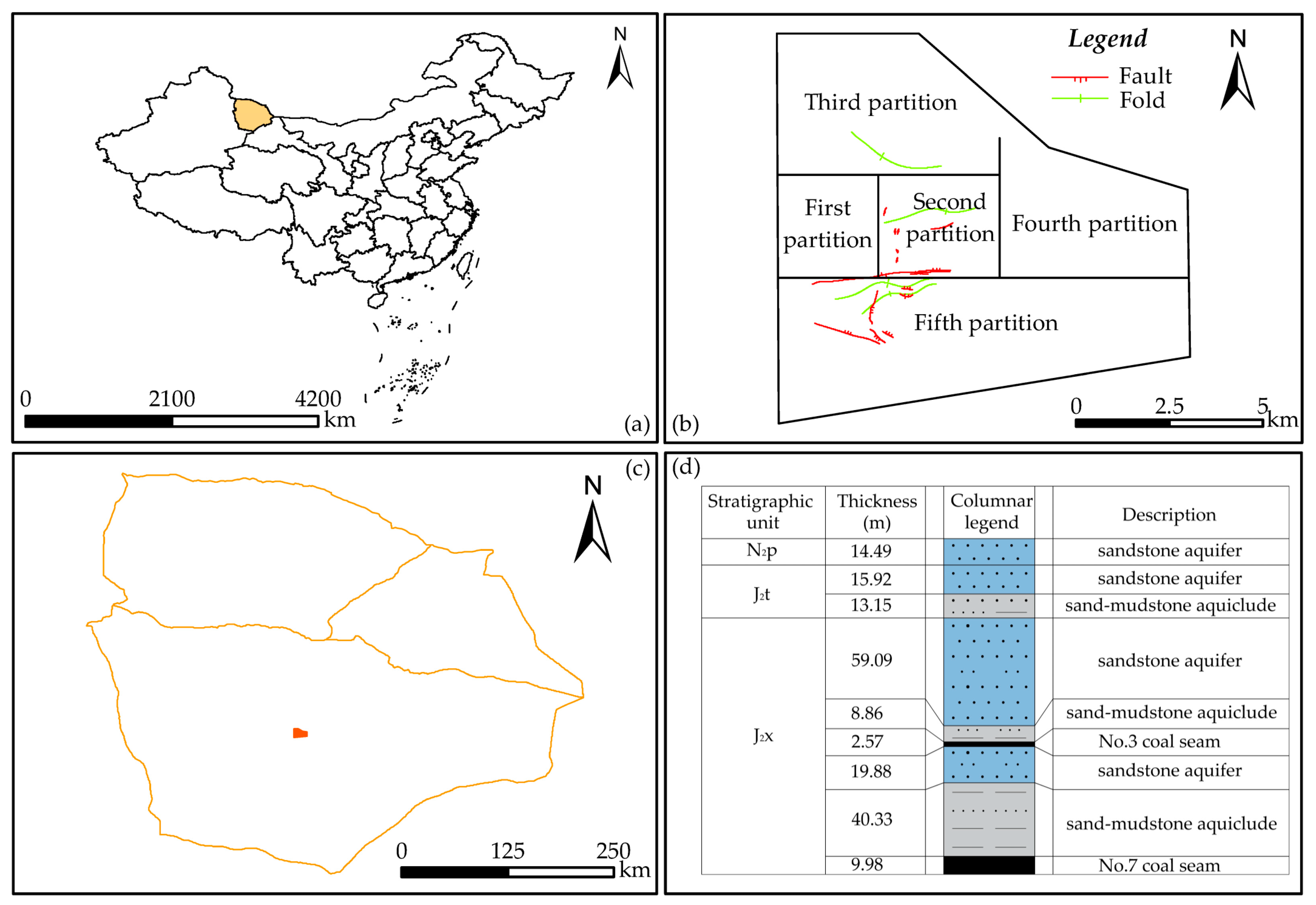
2. Study Area
3. The Primary Determinants of Aquifer Water Abundance
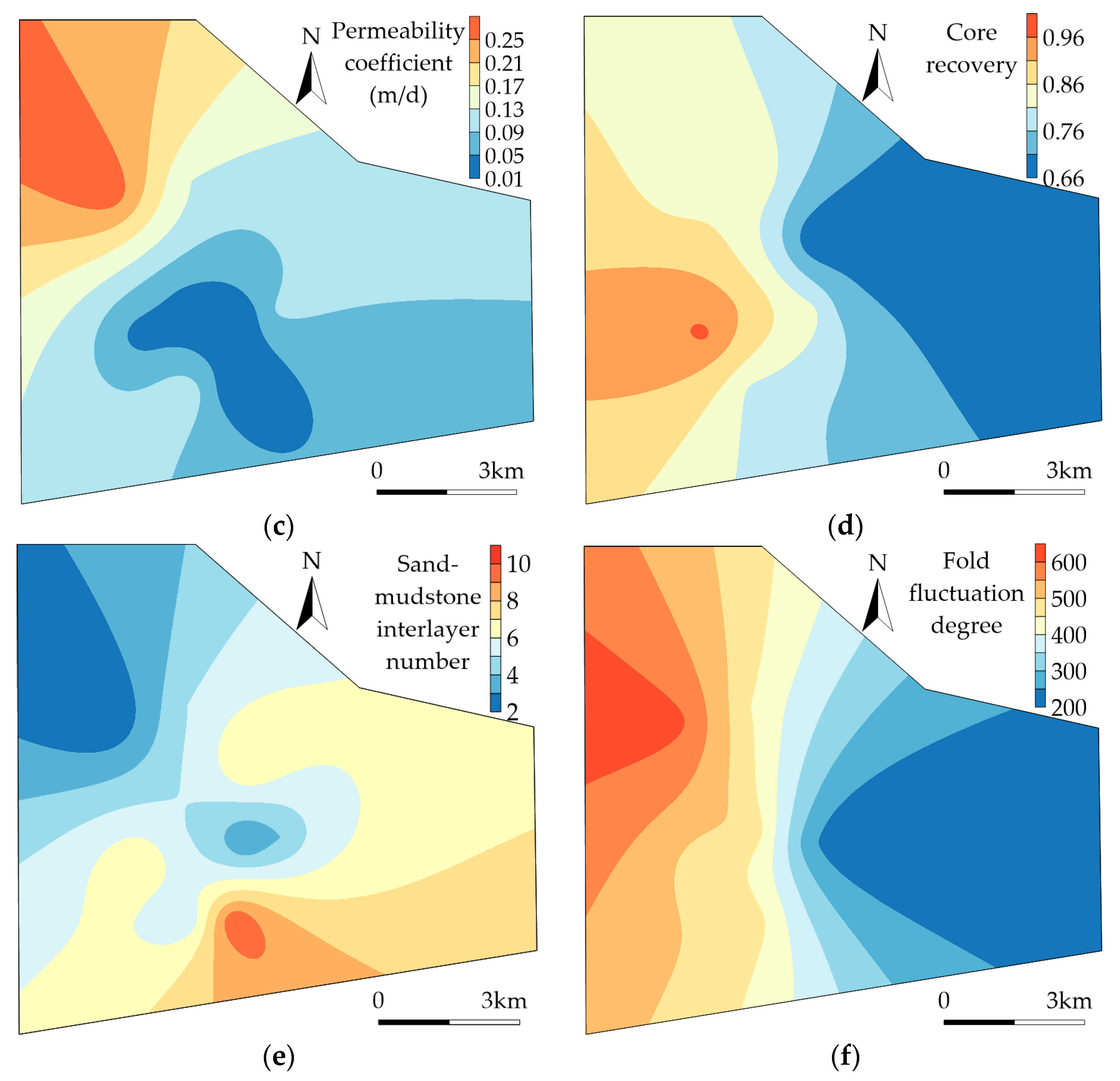
3.1. Analysis of the Main Controlling Factors of Water Abundance
- Aquifer thickness;
- 2.
- Sand (gravel)-mud ratio;
- 3.
- Permeability coefficient;
- 4.
- Core recovery;
- 5.
- Sand-mudstone interlayer number;
- 6.
- Fold fluctuation degree;
3.2. Correlation Analysis of Factors Controlling Water Abundance
4. Model Establishment and Application
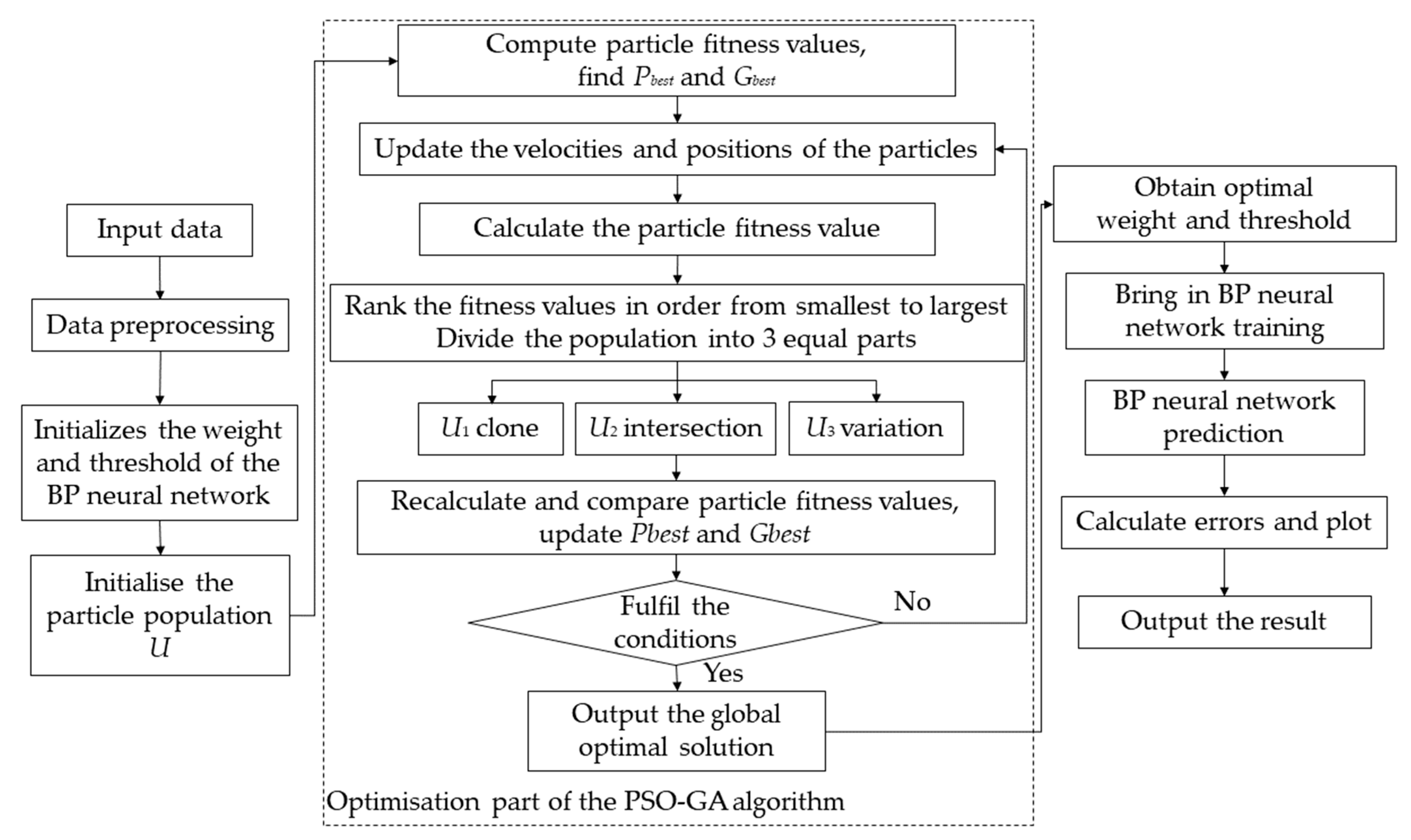
4.1. Principle of PSO-GA-BP Neural Network
- Initialize the particle swarm. Initialize the parameters of the particle swarm, including the particle swarm population size, particle displacement, velocity, individual extreme value and particle swarm extreme value, etc.;
- Calculates the particle fitness value. According to the problem to be solved, the corresponding fitness function is selected, and the individual fitness value of the initial particle swarm is calculated by using the fitness function;
- Update individual extreme value and group extreme value. Comparing the individual adaptation value calculated in the previous step with the individual extreme value of the particle, if the individual adaptation value is better, the individual adaptation value is regarded as the individual optimal position of the population particle, otherwise the original individual extreme value will be maintained until a better individual extreme value appears. Comparing the individual extreme value and the group extreme value, if the individual extreme value is better than the group extreme value, then the individual extreme value is taken as the global optimal position of the particle swarm, otherwise the original group extreme value will be maintained until a better individual extreme value appears;
- Update the position and speed of the particles. Update the position and velocity of particles according to Formulas (3) and (4);
- Judgment of termination conditions. According to the set termination condition of the algorithm, it is judged whether the algorithm meets the end condition, if it does not meet the end condition, return to step 2, and if it meets the end condition, proceed to the next step;
- Output population extremum. The extreme value is regarded as the global optimal solution of the particle swarm optimization.
4.2. Case Analysis
5. Discussion
5.1. FAHP
5.2. Other Neural Network Prediction Models
5.3. Prediction Zoning of Water Abundance
6. Conclusions and Forecast
Author Contributions
Funding
Data Availability Statement
Acknowledgments
Conflicts of Interest
References
- Song, C.Y. Study and Application of Meso-Structural Characteristics and Deformation and Failure Mechanism of Weakly Cemented Sandstone; University of Science and Technology Beijing: Beijing, China, 2017. [Google Scholar]
- Song, C.Y.; Ji, H.G.; Liu, Y.J.; Sun, L.H. Influence factors of driving disturbance of adjacent roadway under the condition of weakly cemented surrounding rock. J. Min. Saf. Eng. 2016, 33, 806–812. [Google Scholar]
- Sun, L.H.; Ji, H.G.; Yang, B.S. Physical and mechanical properties of weakly cemented strata in typical western mining areas. J. Coal 2019, 44, 866–874. [Google Scholar] [CrossRef]
- Dong, S.N.; Ji, Y.D.; Wang, H.; Zhao, B.F.; Cao, H.D. Water disaster prevention and control technology and application of typical roof of Jurassic coalfield in Ordos Basin. J. Coal 2020, 45, 2367–2375. [Google Scholar] [CrossRef]
- Wu, Q.; Xu, K.; Zhang, W. Further discussion on the “Three-map-double prediction method” for predicting and evaluating the risk of water inrush from coal seam roof. J. Coal 2016, 41, 1341–1347. [Google Scholar] [CrossRef]
- Wu, Q.; Huang, X.L.; Dong, D.L.; Yin, Z.R.; Li, J.M.; Hong, Y.Q.; Zhang, H.J. “Three-map-double prediction method” for evaluating water inrush condition of coal seam roof. J. Coal 2000, 25, 62–67. [Google Scholar] [CrossRef]
- Hou, E.K.; Ji, Z.Z.; Che, X.Y.; Wang, J.W.; Gao, L.J.; Tian, S.X.; Yang, F. Water abundance prediction method of weathered bedrock based on improved AHP and entropy weight method. J. Coal Carb. 2019, 44, 3164–3173. [Google Scholar] [CrossRef]
- Li, L.N.; Li, W.P.; Shi, S.Q.; Yang, Z.; He, J.H.; Chen, W.C.; Yang, Y.R.; Zhu, T.E.; Wang, Q.Q. An Improved Potential Groundwater Yield Zonation Method for Sandstone Aquifers and Its Application in Ningxia, China. Nat. Res. Res. 2022, 31, 849–865. [Google Scholar] [CrossRef]
- Lu, Q.Y.; Li, X.Q.; Li, W.P.; Chen, W.; Li, L.F.; Liu, S.L. Risk Evaluation of Bed-Separation Water Inrush: A Case Study in the Yangliu Coal Mine, China. Mine Water Environ. 2018, 37, 288–299. [Google Scholar] [CrossRef]
- Xue, S.; Li, W.P.; Guo, Q.C.; Liu, S.L.; Sun, M.Y.; Fan, B.J. Prediction of water abundance of roof confined aquifer based on FAHP-GRA evaluation method. Metal. Mine 2018, 4, 168–172. [Google Scholar]
- Gong, H.J.; Zeng, Y.F.; Liu, S.Q.; Li, Z.; Niu, P.K. Evaluation of aquifer abundance based on improved fuzzy analytic hierarchy process. Coal Technol. 2018, 37, 158–159. [Google Scholar]
- Al-Abadi, A.M.; Shahid, A. A comparison between index of entropy and catastrophe theory methods for mapping groundwater potential in an arid region. Environ. Monit. Assess. 2015, 187, 576. [Google Scholar] [CrossRef]
- Jenifer, M.A.; Jha, M.K. Comparison of Analytic Hierarchy Process, Catastrophe and Entropy techniques for evaluating groundwater prospect of hard-rock aquifer systems. J. Hydrol. 2017, 548, 605–624. [Google Scholar] [CrossRef]
- Wu, Q.; Fan, Z.L.; Liu, S.Q.; Zhang, Y.W.; Sun, W.J. Evaluation method of water abundance of information fusion aquifer based on GIS-water abundance index method. J. Coal 2011, 36, 1124–1128. [Google Scholar] [CrossRef]
- Wu, Q.; Wang, J.H.; Liu, D.H.; Cui, F.P.; Liu, S.Q. A new practical method for evaluating water inrush from coal seam floor IV: Application of AHP vulnerability index method based on GIS. J. Coal 2009, 34, 233–238. [Google Scholar] [CrossRef]
- Han, C.; Pan, X.H.; Li, G.L.; Tu, J.N. Fuzzy Analytic hierarchy process of aquifer Water abundance based on GIS Multi-source Information Integration. Hydrogeol. Eng. Geol. 2012, 39, 19–25. [Google Scholar]
- Wang, G.D. Study on aquifer water abundance based on fuzzy analytic hierarchy process. Coal Technol. 2016, 35, 209–210. [Google Scholar]
- Rahmati, O.; Samani, A.N.; Mahdavi, M.; Pourghasemi, H.R.; Zeinivand, H. Groundwater potential mapping at Kurdistan region of Iran using analytic hierarchy process and GIS. Arab. J. Geosci. 2015, 8, 7059–7071. [Google Scholar] [CrossRef]
- Machiwal, D.; Rangi, N.; Sharma, A. Integrated knowledge- and data-driven approaches for groundwater potential zoning using GIS and multi-criteria decision making techniques on hard-rock terrain of Ahar catchment, Rajasthan, India. Environ. Earth Sci. 2015, 73, 1871–1892. [Google Scholar] [CrossRef]
- Gong, H.J.; Liu, S.Q.; Zeng, Y.F. Study on evaluation of aquifer abundance based on BP neural network. Coal Technol. 2018, 37, 181–182. [Google Scholar]
- Li, Z.; Zeng, Y.F.; Liu, S.Q.; Gong, H.J.; Niu, P.K. Application of BP artificial neural network in water abundance evaluation. Coal Eng. 2018, 50, 114–118. [Google Scholar]
- Jiang, S.; Sun, Y.J.; Yang, L.; Lin, C.P. Prediction of mine water inflow based on BP neural network method. Coal Geol. Chin. 2007, 19, 38–40. [Google Scholar]
- Ling, C.P.; Sun, Y.J.; Yang, L.H.; Jiang, S.; Shao, F.Y. Prediction of water inflow from pore-filled mine based on BP neural network. Hydrogeology 2007, 55–58. Available online: http://www.swdzgcdz.cn/index.php?m=content&c=index&a=show&catid=72&id=1746 (accessed on 21 November 2023).
- Xiao, Z.X. Study on Prediction of Water Inflow from Underwater Tunnel Based on Genetic Algorithm and Neural Network; Southwest Jiaotong University: Chengdu, China, 2011. [Google Scholar]
- Xiao, Z.X.; Huang, T.; Li, Z.; Pan, M.M. Application of genetic-neural network algorithm in prediction of water inflow from underwater tunnel. J. Water Res. Water Eng. 2011, 22, 102–105. [Google Scholar]
- Li, Z.Y.; Wang, Y.C.; Olgun, C.G.; Yang, S.Q.; Jiao, Q.L.; Wang, M.T. Risk assessment of water inrush caused by karst cave in tunnels based on reliability and GA-BP neural network. Geomat. Nat. Hazards Risk 2020, 11, 1212–1232. [Google Scholar] [CrossRef]
- Wu, Q.; Wang, Y.; Zhao, D.K.; Shen, J.J. Evaluation method and application of water abundance of loose aquifer based on sedimentary characteristics. J. Chin. Univ. Min. Technol. 2017, 46, 460–466. [Google Scholar]
- Chen, Z.F. Evaluation of the effectiveness of China’s Monetary Policy—An Analysis based on Pearson correlation coefficient. Chin. Busin. Theory 2020, 6, 48–49. [Google Scholar]
- Yang, F.; Feng, X.; Ruan, L.; Chen, J.W.; Xia, R.; Chen, Y.L.; Jin, Z.H. Study on the correlation between water branches and ultra-low frequency dielectric loss based on Pearson correlation coefficient method. High Volt. Elec. Appl. 2014, 50, 21–25+31. [Google Scholar]
- Bashir, Z.A.; El-Hawary, M.E. Applying Wavelets to Short-Term Load Forecasting Using PSO-Based Neural Networks. IEEE Trans. Power Syst. 2009, 24, 20–27. [Google Scholar] [CrossRef]
- Momeni, E.; Jahed, A.D.; Hajihassani, M.; Mohd, M.A. Prediction of uniaxial compressive strength of rock samples using hybrid particle swarm optimization-based artificial neural networks. Measurement 2015, 60, 50–63. [Google Scholar] [CrossRef]
- Ao, Y.C.; Shi, Y.B.; Zhang, W.; Li, Y.J. Improved particle swarm optimization algorithm with adaptive inertia weight. J. Univ. Elect. Sci. Technol. 2014, 43, 874–880. [Google Scholar]
- Zhang, H.; Wang, X.L. Particle swarm optimization algorithm for adaptive inertia weight optimization. Intel. Comp. Appl. 2023, 13, 5–8. [Google Scholar]
- Zhang, Y.B.; Zou, D.X.; Zhang, C.Y.; Du, X.H. Particle swarm optimization algorithm with adaptive inertia weight. Comput. Simul. 2023, 40, 350–357. [Google Scholar]


| Aquifer Thickness | Sand (Gravel)- Mud Ratio | Permeability Coefficient | Core Recovery | Sand-Mudstone Interlayer Number | Fold Fluctuation Degree | |
|---|---|---|---|---|---|---|
| Aquifer thickness | 1 | |||||
| Sand (gravel)-mud ratio | 0.105 | 1 | ||||
| Permeability coefficient | 0.129 | 0.781 * | 1 | |||
| Core recovery | 0.136 | 0.113 | −0.097 | 1 | ||
| Sand-mudstone interlayer number | −0.055 | −0.617 | −0.601 | −0.118 | 1 | |
| Fold fluctuation degree | −0.182 | 0.556 | 0.549 | 0.520 | −0.152 | 1 |
| Sample Number | Actual Value L/(s·m) | Water Abundance Class | Predicted Value L/(s·m) | Water Abundance Class | Error |
|---|---|---|---|---|---|
| 1 | 0.1659 | Medium | 0.1537 | Medium | −0.0122 |
| 2 | 0.04 | Weak | 0.0997 | Weak | 0.0597 |
| 3 | 0.0097 | Weak | 0.0684 | Weak | 0.0587 |
| 4 | 0.1887 | Medium | 0.1434 | Medium | −0.0453 |
| 5 | 0.0198 | Weak | 0.0968 | Weak | 0.0770 |
| 6 | 0.0406 | Weak | 0.1087 | Medium | 0.0681 |
| 7 | 0.0077 | Weak | 0.1034 | Medium | 0.0957 |
| 8 | 0.1196 | Medium | 0.1128 | Medium | −0.0068 |
| 9 | 0.0316 | Weak | 0.1132 | Medium | 0.0816 |
| Sample Number | Actual Value | BP | BP Error | GA-BP | GA-BP Error | PSO-GA-BP | PSO-GA-BP Error |
|---|---|---|---|---|---|---|---|
| 1 | 0.1659 | 0.1653 | −0.00063 | 0.1662 | 2.86 × 10⁻⁴ | 0.1658 | −4.27 × 10⁻⁵ |
| 2 | 0.0401 | 0.0447 | 0.00460 | 0.0377 | −2.39 × 10⁻³ | 0.0401 | 1.65 × 10⁻⁵ |
| 3 | 0.0098 | 0.0263 | 0.01655 | 0.0150 | 5.26 × 10⁻³ | 0.0098 | 6.66 × 10⁻⁸ |
| 4 | 0.1887 | 0.1870 | −0.00104 | 0.1876 | −1.65 × 10⁻³ | 0.1875 | −1.14 × 10⁻³ |
| 5 | 0.0198 | 0.0219 | 0.00211 | 0.0217 | 1.89 × 10⁻³ | 0.0198 | 3.57 × 10⁻⁵ |
| 6 | 0.0406 | 0.0449 | 0.00438 | 0.0393 | −1.23 × 10⁻³ | 0.0405 | −3.53 × 10⁻⁵ |
| 7 | 0.0077 | 0.0146 | 0.00684 | 0.0067 | −1.01 × 10⁻³ | 0.0077 | −5.01 × 10⁻⁶ |
| 8 | 0.1195 | 0.1160 | −0.00352 | 0.1188 | −7.06 × 10⁻⁴ | 0.1194 | −8.88 × 10⁻⁵ |
| 9 | 0.0316 | 0.0479 | 0.01629 | 0.0317 | 1.03 × 10⁻⁴ | 0.0315 | −6.86 × 10⁻⁵ |
Disclaimer/Publisher’s Note: The statements, opinions and data contained in all publications are solely those of the individual author(s) and contributor(s) and not of MDPI and/or the editor(s). MDPI and/or the editor(s) disclaim responsibility for any injury to people or property resulting from any ideas, methods, instructions or products referred to in the content. |
© 2023 by the authors. Licensee MDPI, Basel, Switzerland. This article is an open access article distributed under the terms and conditions of the Creative Commons Attribution (CC BY) license (https://creativecommons.org/licenses/by/4.0/).
Share and Cite
Dai, X.; Li, X.; Zhang, Y.; Li, W.; Meng, X.; Li, L.; Han, Y. A Prediction Model of Coal Seam Roof Water Abundance Based on PSO-GA-BP Neural Network. Water 2023, 15, 4117. https://doi.org/10.3390/w15234117
Dai X, Li X, Zhang Y, Li W, Meng X, Li L, Han Y. A Prediction Model of Coal Seam Roof Water Abundance Based on PSO-GA-BP Neural Network. Water. 2023; 15(23):4117. https://doi.org/10.3390/w15234117
Chicago/Turabian StyleDai, Xue, Xiaoqin Li, Yuguang Zhang, Wenping Li, Xiangsheng Meng, Liangning Li, and Yanbo Han. 2023. "A Prediction Model of Coal Seam Roof Water Abundance Based on PSO-GA-BP Neural Network" Water 15, no. 23: 4117. https://doi.org/10.3390/w15234117