
A Developed Multiple Linear Regression (MLR) Model for Monthly Groundwater Level Prediction

Abstract
:1. Introduction
- An advanced machine learning model is developed to predict the monthly GWL. We combine three models to predict monthly groundwater levels. As our proposed model consists of two robust deep learning models, it can be superior to linear models such as MLR models. Since our proposed model uses the capabilities of CNN and LSTM models simultaneously, it outperforms standalone CNN and LSTM models. The CLM model is presented as a reliable tool for predicting GWLs in different basins. Since it can be adapted to different watersheds, it can be a reliable tool for water resource managers around the world.
- A new optimizer is introduced to identify the best input combination. An optimization algorithm determines the best input combination, while the correlation method only determines important inputs. To identify the most optimal set of features, the new method performs an extensive search and explores various combinations. The new optimization method handles high-dimensional feature spaces and can be fine-tuned to maximize model accuracy, minimize error, or enhance specific evaluation metrics. As a result, our study contributes to feature selection.
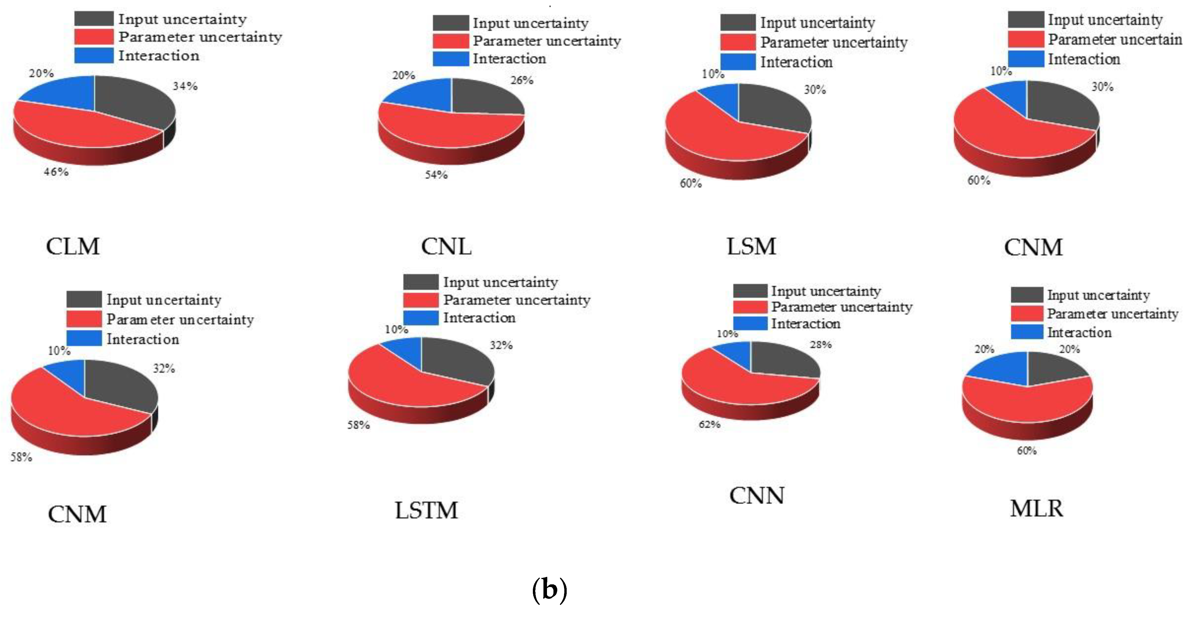
- An effective method is suggested to quantify uncertainty values. This study contributes to the quantification of output uncertainty values. The study illustrates how model parameters and inputs contribute to model uncertainties. Through the analysis of variance (ANOVA) method, the study provides insight into the sources and values of output uncertainty.
- We use an advanced method to decompose the output uncertainty into different sources of uncertainty. Our study proposes a new method to calculate the percentage contribution of inputs and model parameters to overall uncertainty.
2. Materials and Methods
2.1. MLR Model
2.2. Mathematical Model of the LSTM
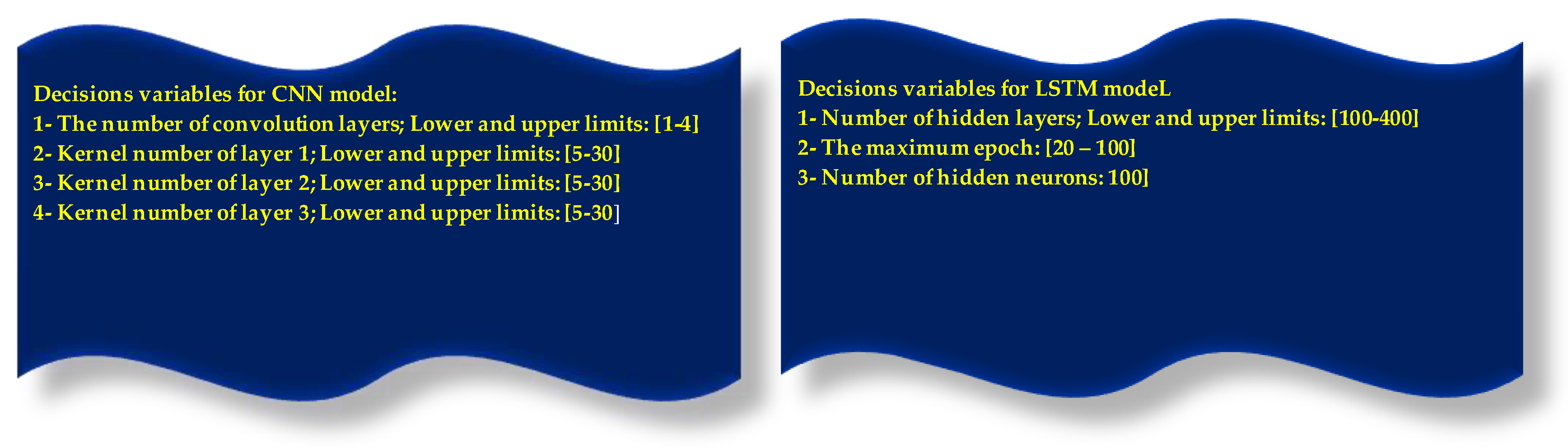
2.3. Mathematical Model of the CNN Model
2.4. Input Selection
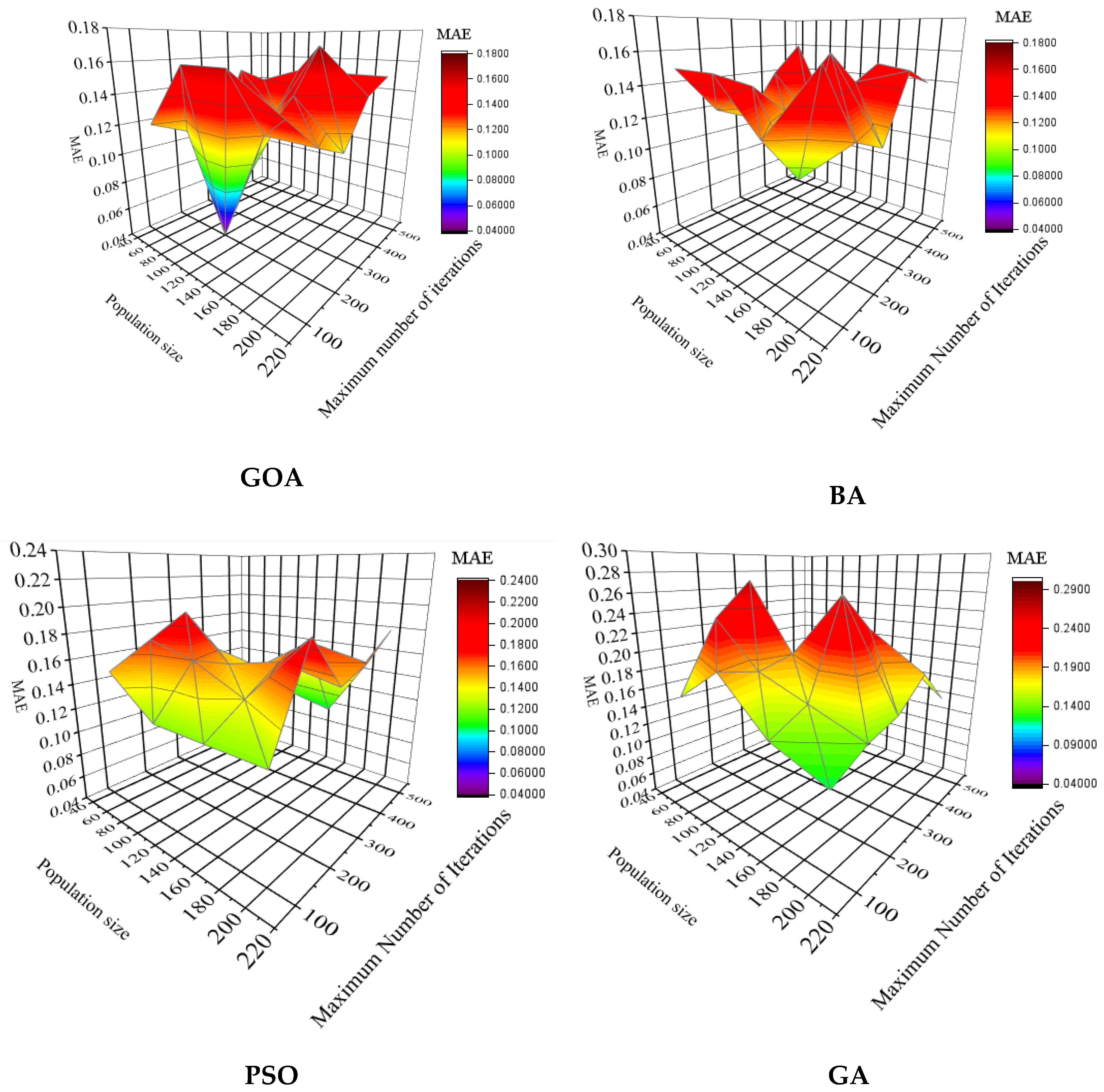
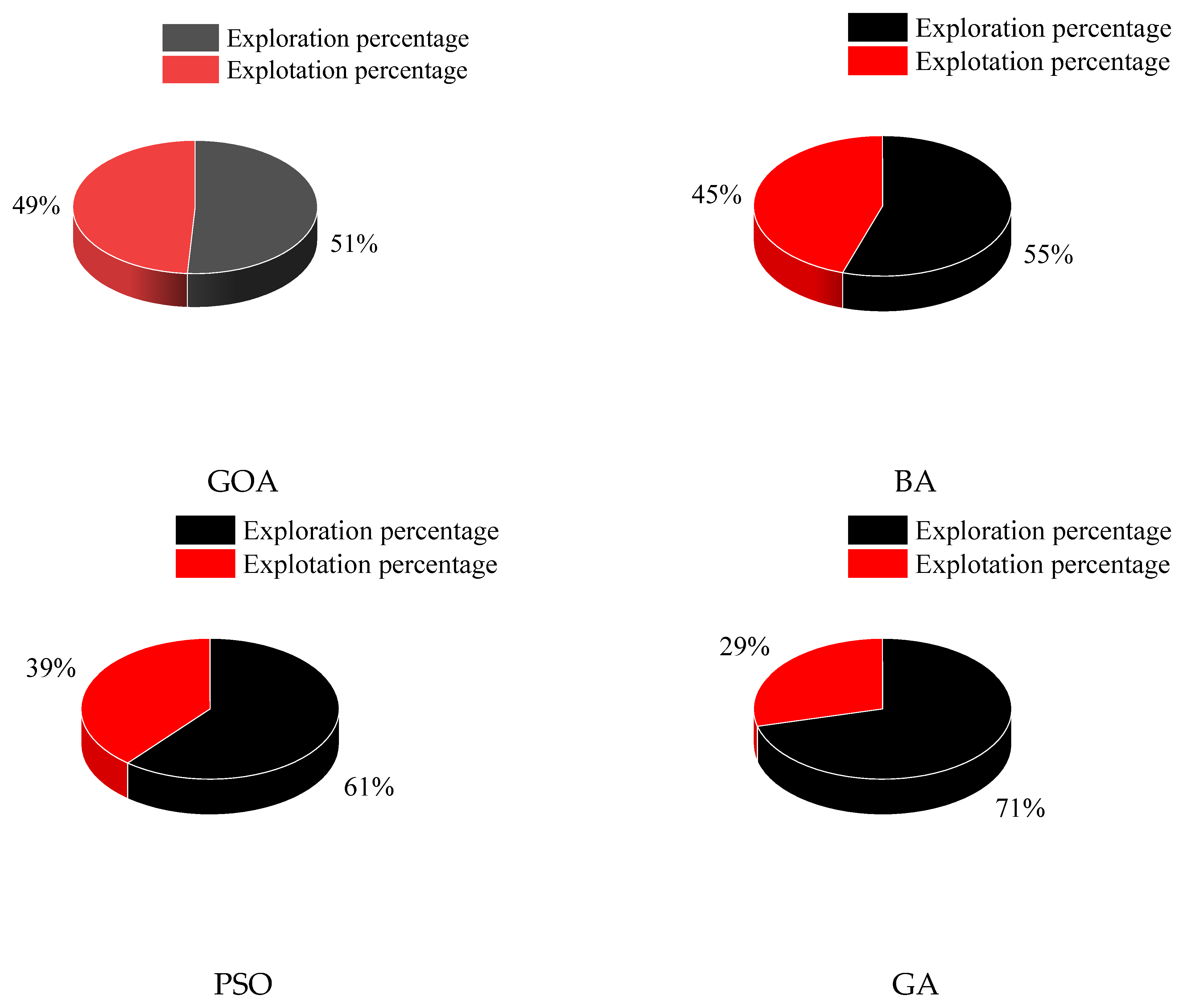
2.4.1. Structure of GOA
2.4.2. Bat Algorithm (BA)
2.4.3. Particle Swarm Optimization (PSO)
2.4.4. Genetic Algorithm (GA)
2.4.5. Binary Version of Optimization Algorithms
2.5. Hybrid CLM Model for Predicting GWL
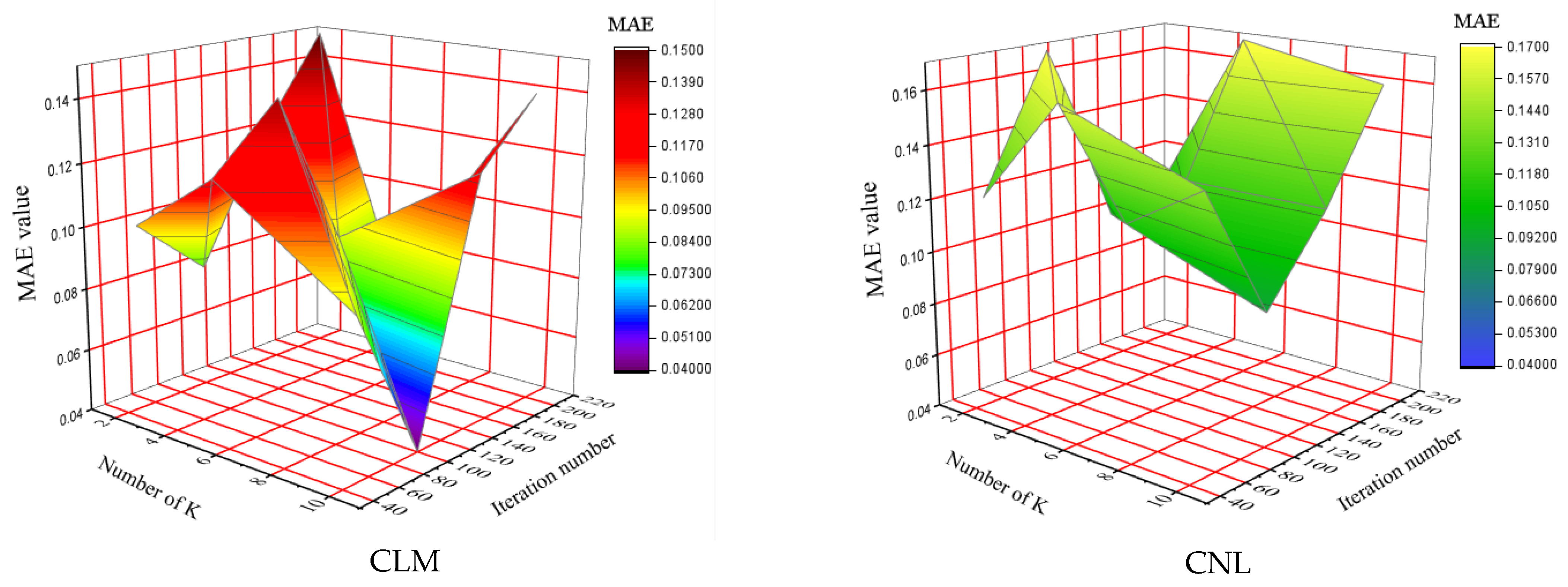
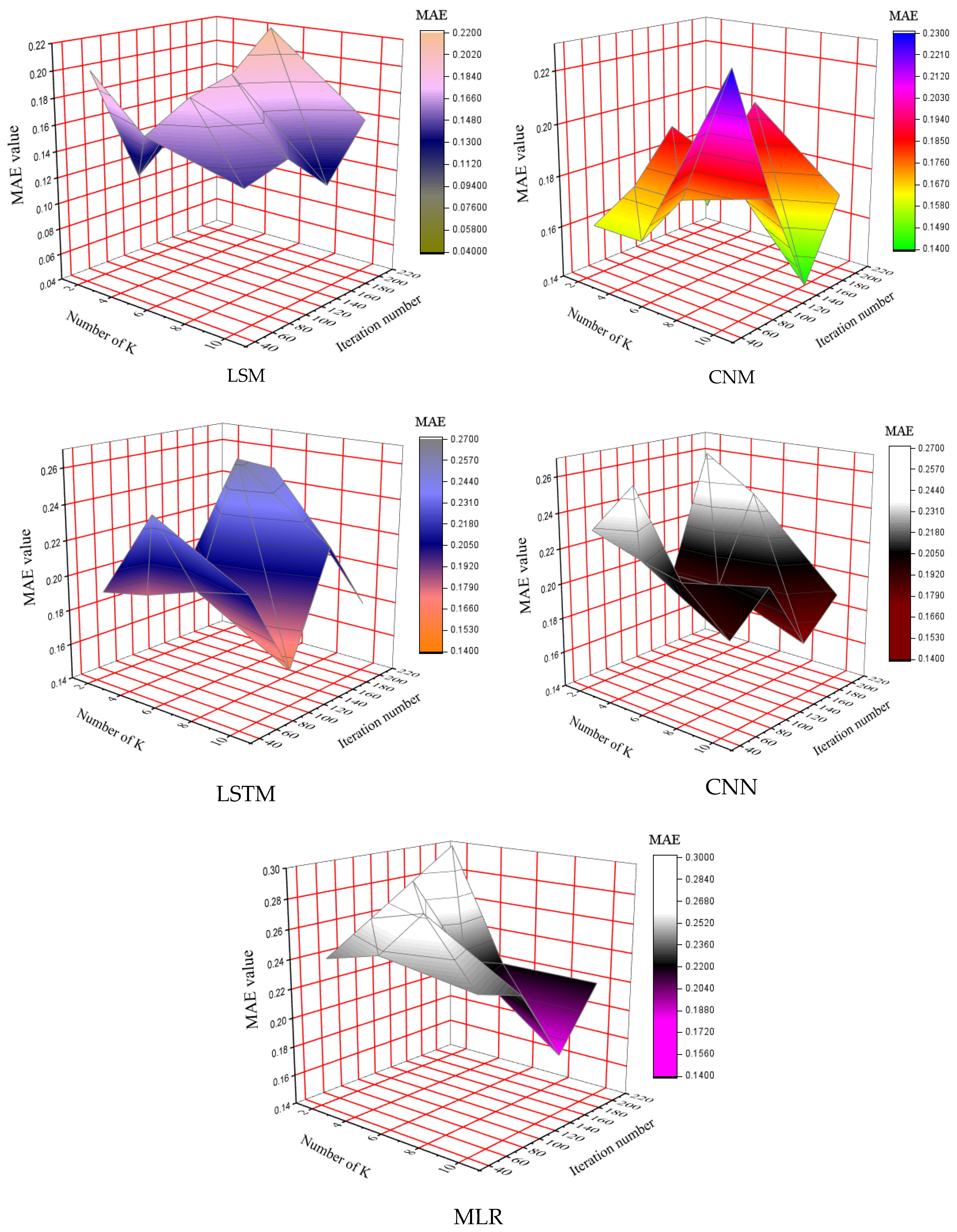
- The parameters of the CNN model and the names of the inputs are initialized as the initial population of the binary GOA. In the modeling process, it is important to determine the training and testing data. K-fold cross-validation (KCV) is one of the suitable methods for partitioning input data into training and testing datasets [37]. The KCV method evaluates model accuracy by dividing data into K folds. Training data are divided into K-1 folds. Finally, the model is run K times to calculate the average error function. The average error function value is used to evaluate model performance and determine the optimal number of folds [38].
- Each possible input scenario is encoded as a binary string. Each bit represents the presence (1) or absence (0) of a specific input variable. An initial population of potential solutions (binary strings) is generated. These strings represent various combinations of input variables. The binary string 11,111 indicates that all inputs are considered during modeling. The algorithm can identify the most influential input combinations based on the defined fitness function by exploring various combinations and evaluating their performance.
- The CNN model is executed by using training data.
- CNN is run in the testing phase if termination criteria are met; otherwise, CNN is connected to GOA. CNN parameters and input names are updated using optimization algorithms.
- LSTM models use CNN outputs as inputs. The LSTM model is run using training data. The LSTM parameters are defined as the initial population of optimizers. The LSTM model is run at the testing level if the termination criteria are met; otherwise, the GOA is connected to the LSTM mode.
- MLR uses the outputs of the LSTM model as inputs. The LSTM model extracts temporal features from time series data. Temporal features can capture relationships between different data points. Then, the extracted features are sent to the MLR model to predict GWLs. The MLR model produces final outputs.
2.6. Quantitation of Uncertainty Values
2.7. Determination of Contribution of Input Parameters and Models to Output Uncertainty
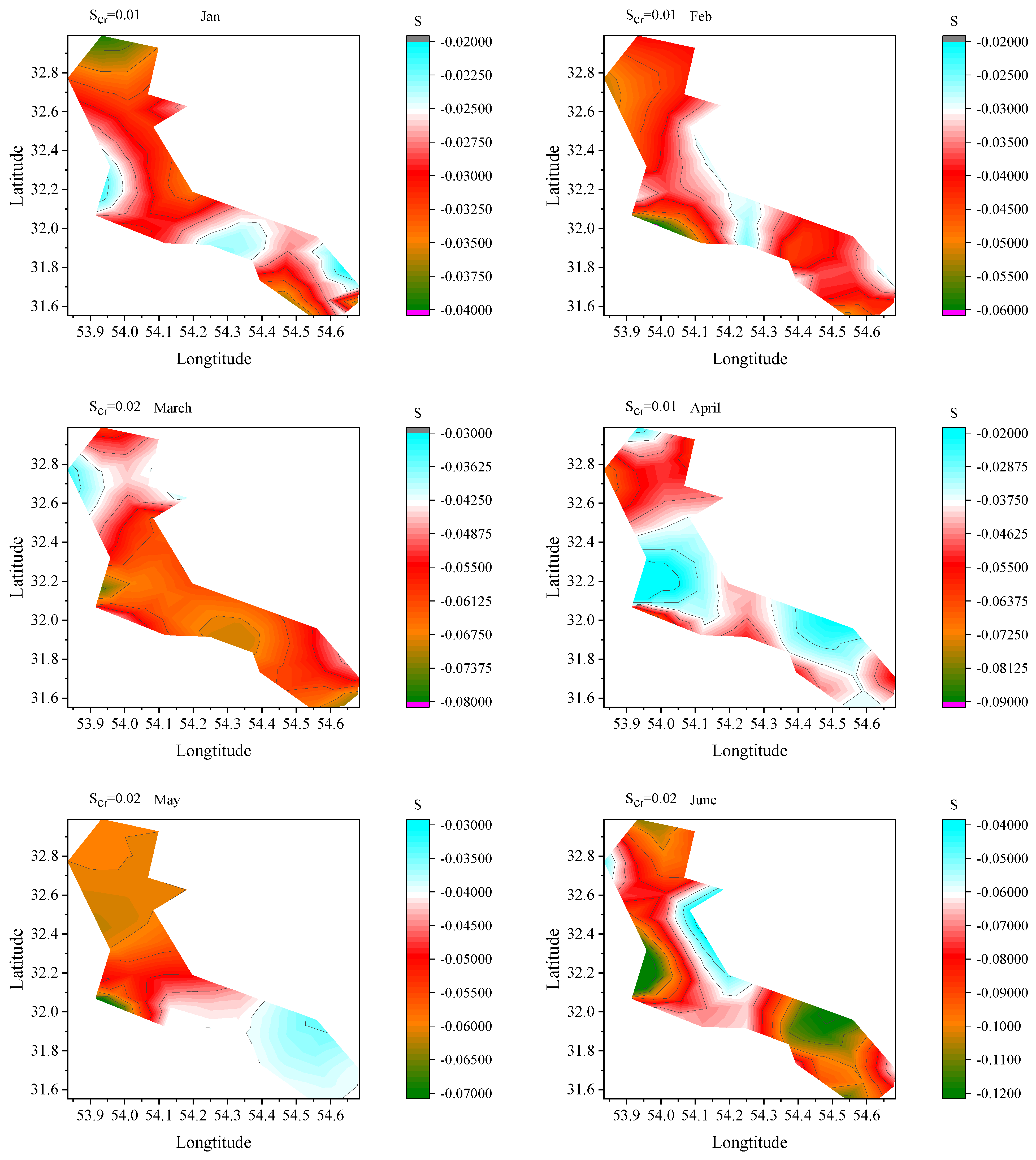
2.8. Trend Analysis
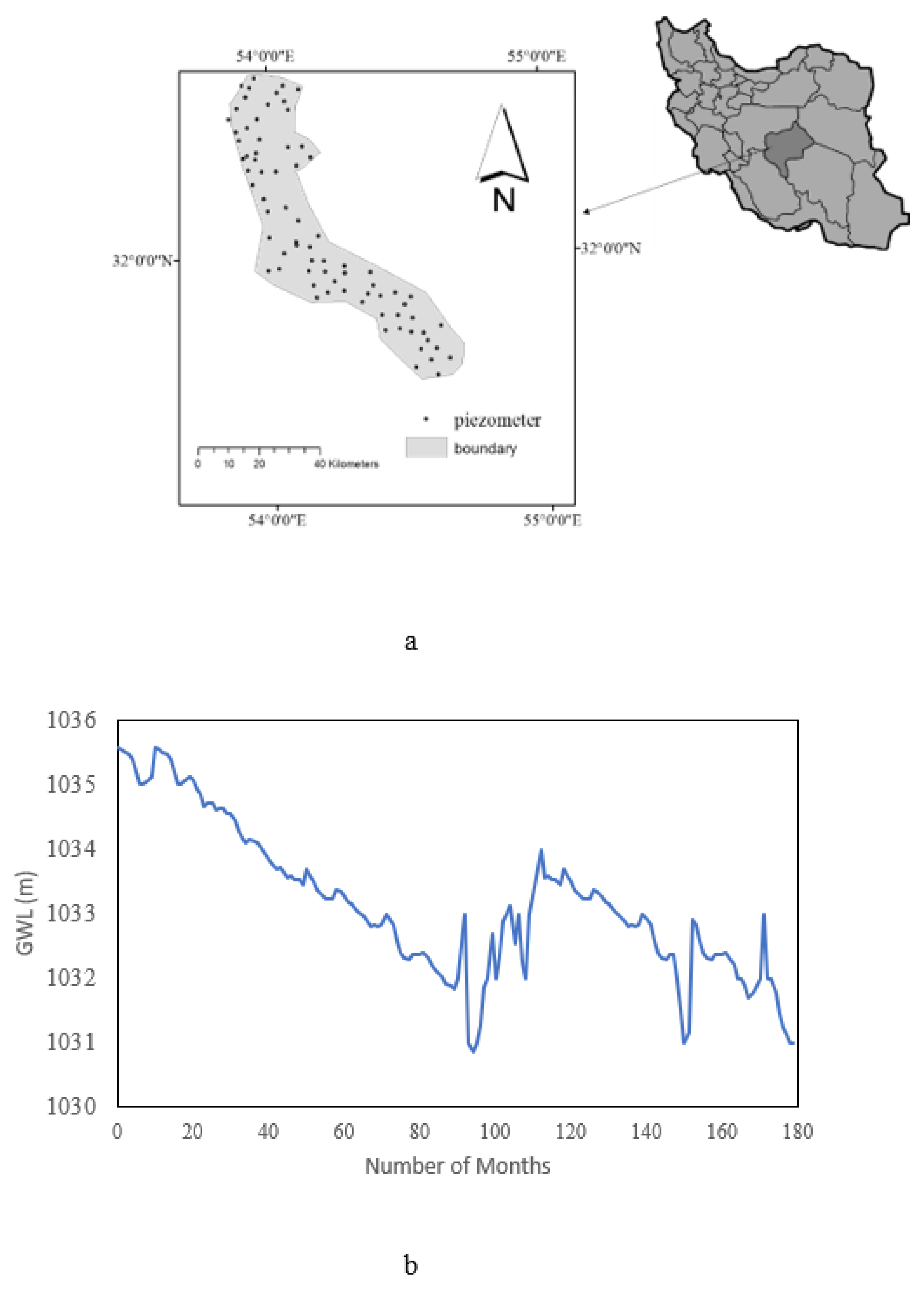
3. Case Study
3.1. Details of Case Study
- Root mean square error (RMSE)
- Mean absolute error (MAE)
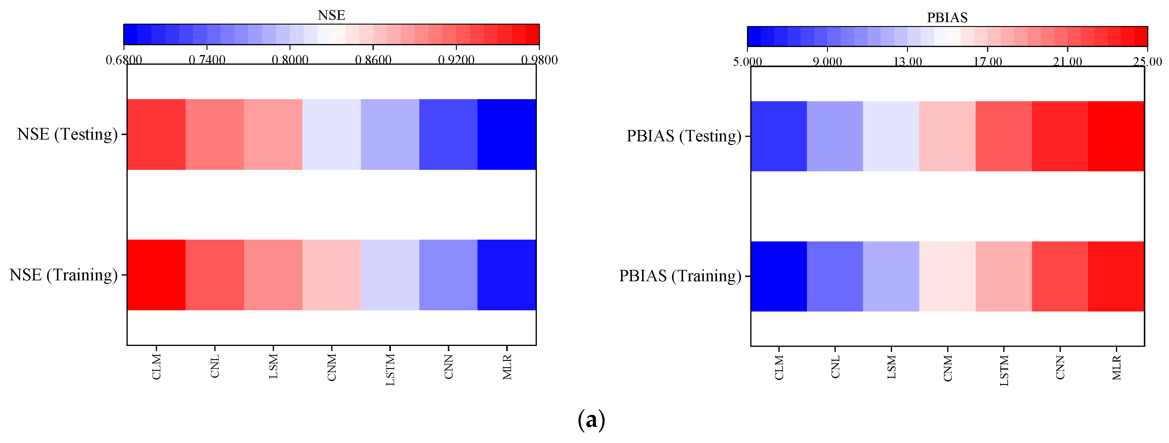
- Nash Sutcliffe efficiency (NSE)
- Percent bias (PBIAS)
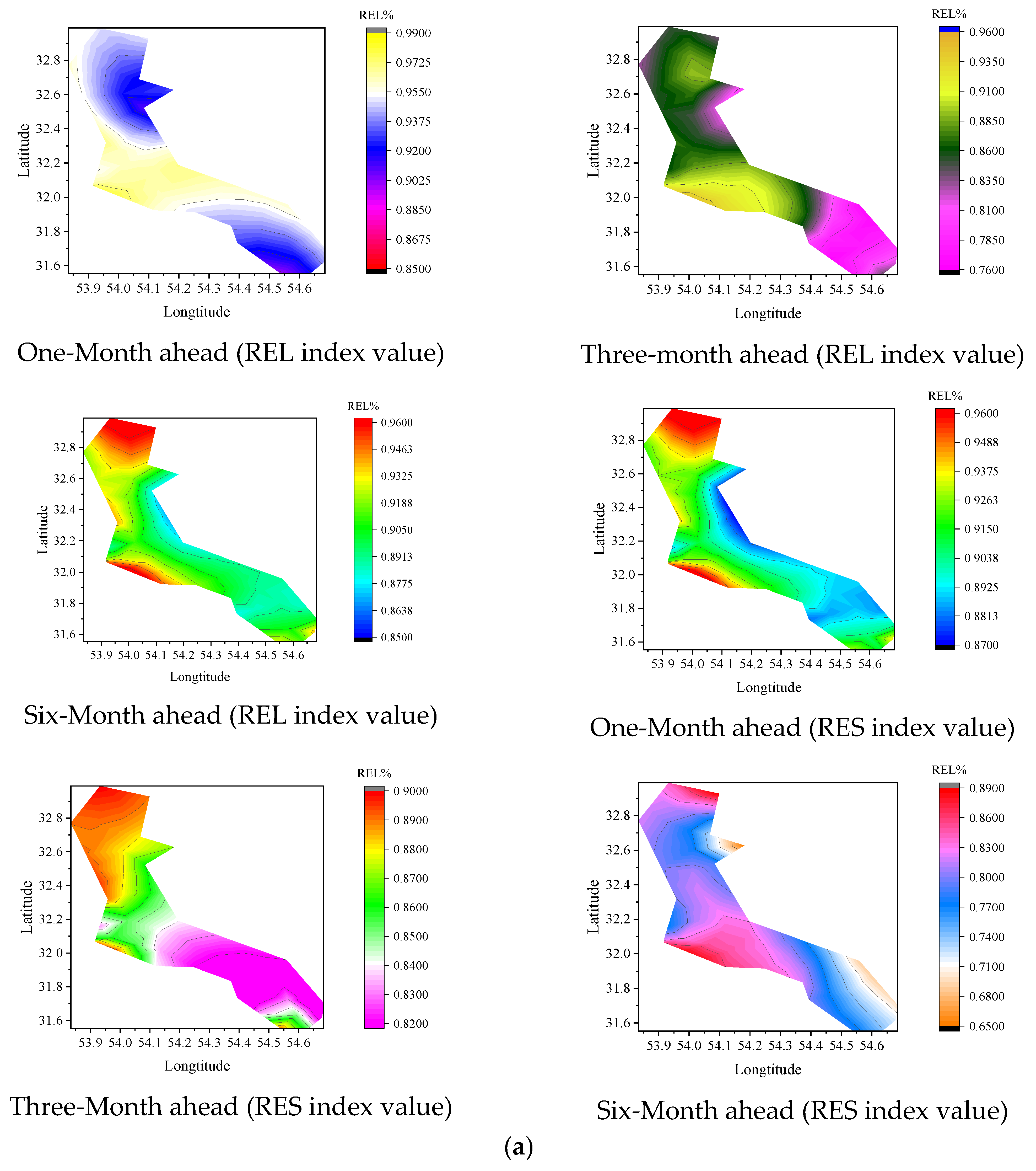
- Reliability index (REI)
- Resiliency index (RES)where : estimated GWL; : observed data; N: the number of data; and : a constant value ( based on the Chinese standard = 0.20). Equations (55)–(57) are applied to quantify uncertainty values.
- Width interval (WI)
- Prediction interval coverage probability (PICP)where and : upper and lower values of variables, : observed data, and R: the difference between maximum and minimum values.
3.2. Error Function for Evaluating the Performance of Optimization Algorithms in Choosing Inputs
4. Results
4.1. Determination of Algorithm Parameters
4.2. Determination of Number of Folds (K)
4.3. Selection of the Best Optimization Algorithm for Choosing Inputs
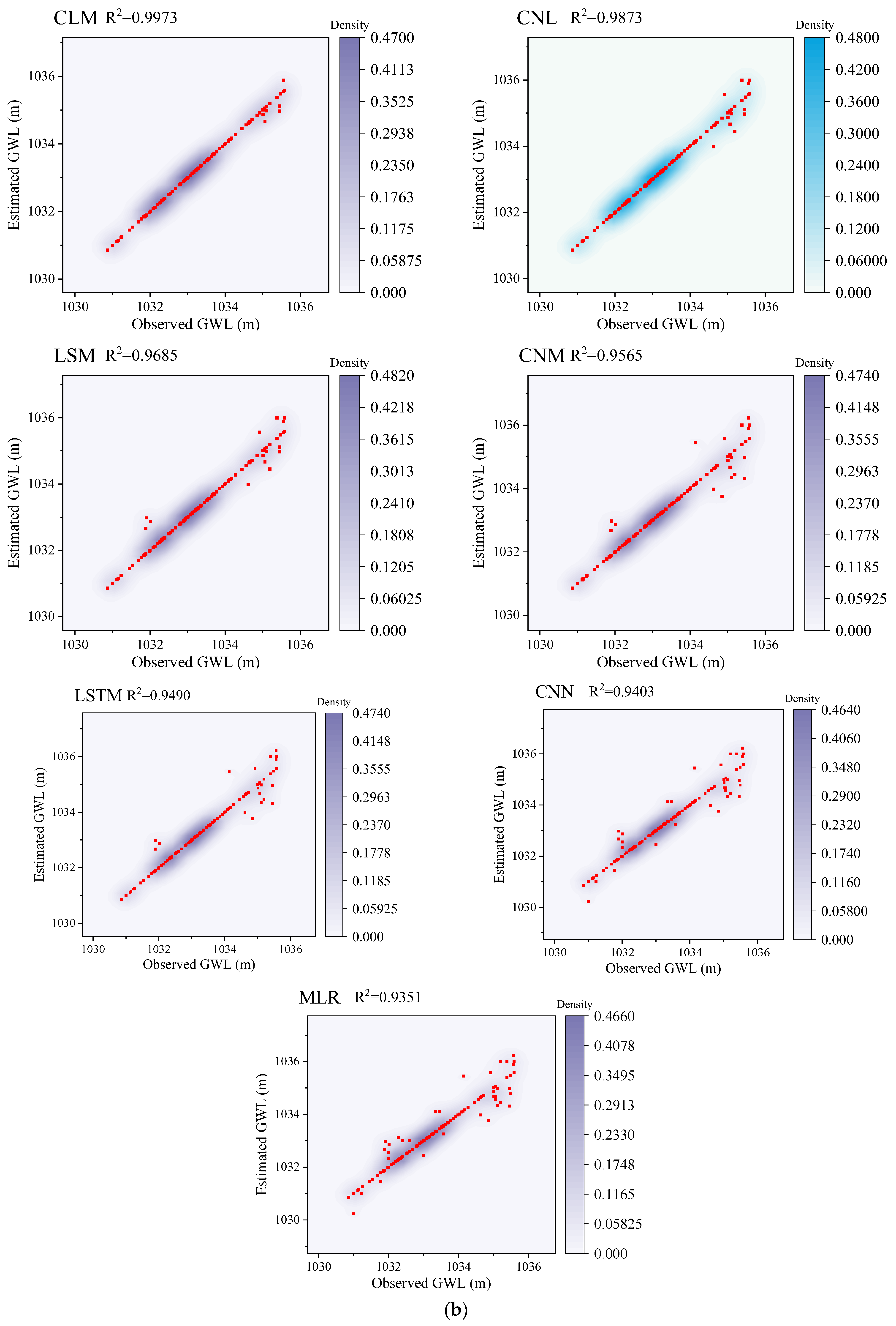
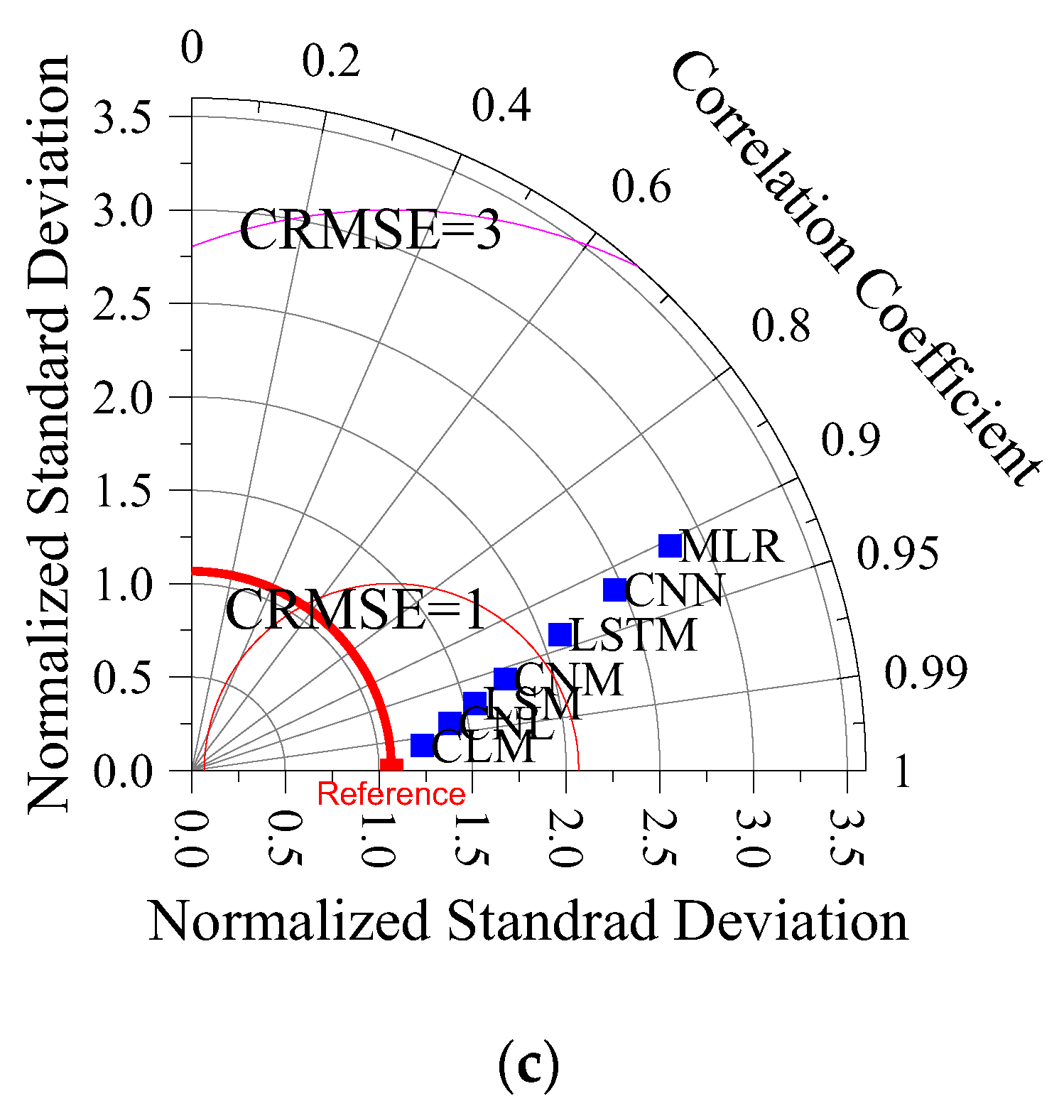
4.4. Evaluation of the Performance of Predictive Models in Predicting GWL
5. Discussion
5.1. Evaluation of the Accuracy of Models for Different Horizon Predictions
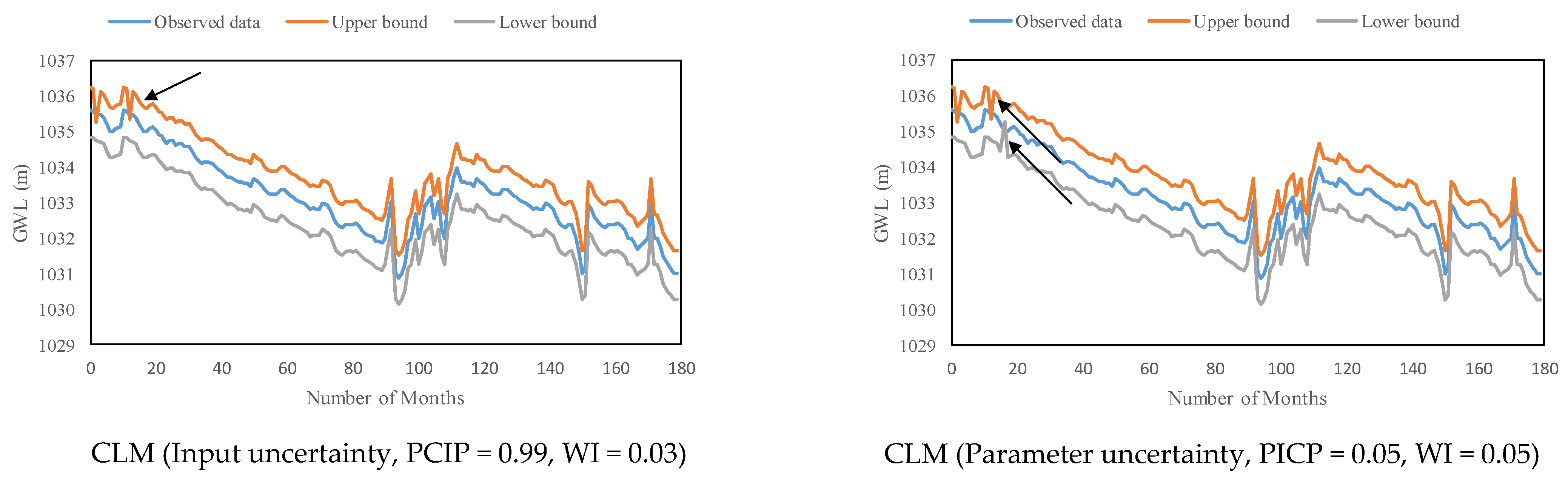
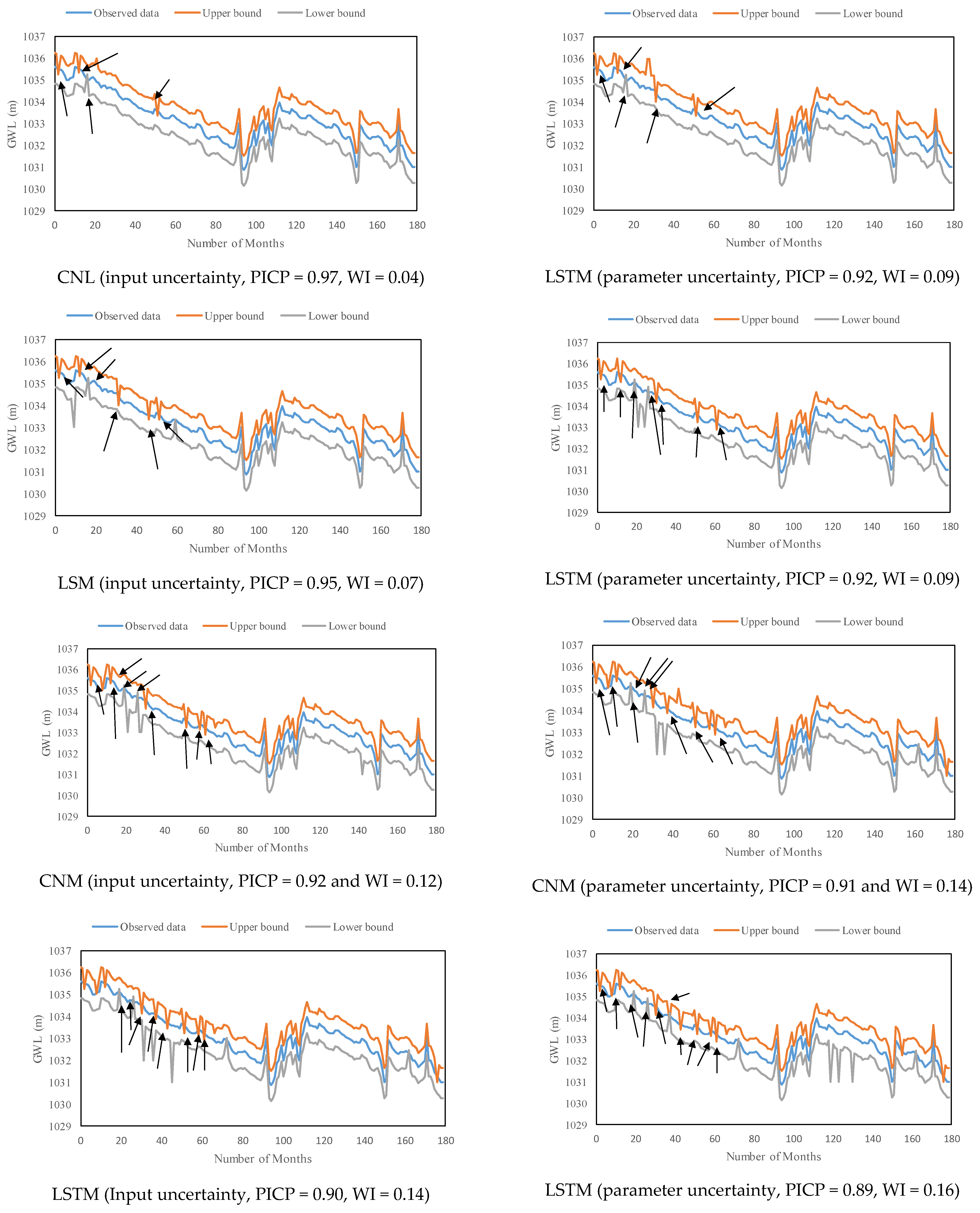
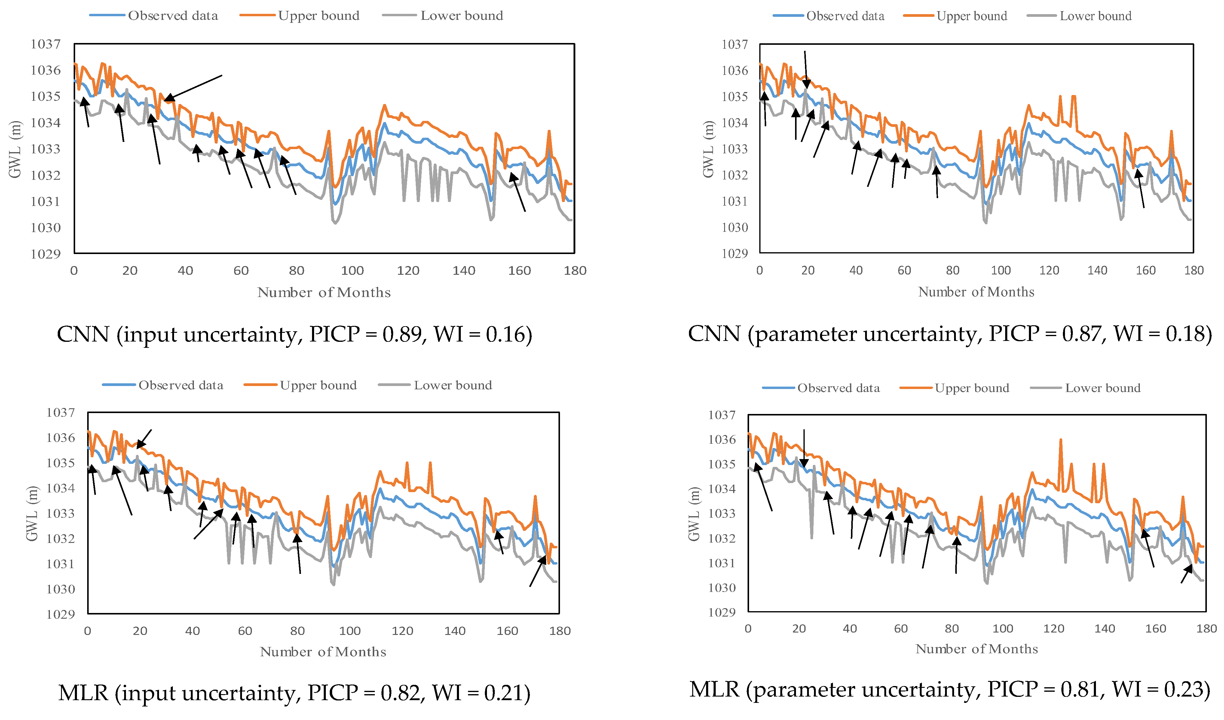
5.2. The Contribution of Input and Parameter Uncertainty to the Output Uncertainty
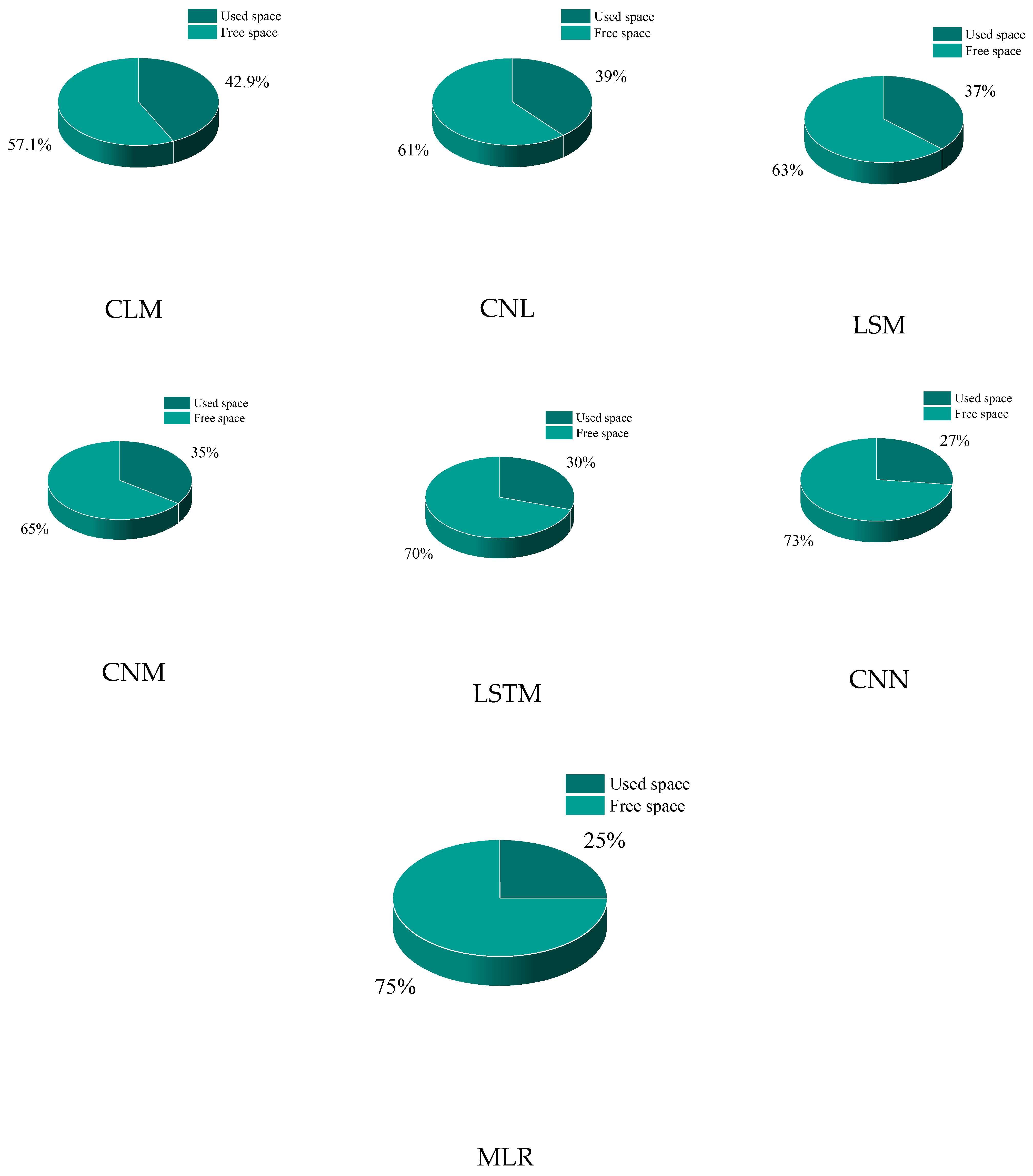
5.3. Memory Usage Percentage of Models
5.4. Trend Defection
6. Conclusions
Author Contributions
Funding
Data Availability Statement
Conflicts of Interest
References
- Tao, H.; Hameed, M.M.; Marhoon, H.A.; Zounemat-Kermani, M.; Heddam, S.; Kim, S.; Sulaiman, S.O.; Tan, M.L.; Sa’adi, Z.; Mehr, A.D.; et al. Groundwater Level Prediction Using Machine Learning Models: A Comprehensive Review. Neurocomputing 2022, 489, 271–308. [Google Scholar] [CrossRef]
- Di Nunno, F.; Granata, F. Groundwater Level Prediction in Apulia Region (Southern Italy) Using NARX Neural Network. Environ. Res. 2020, 190, 110062. [Google Scholar] [CrossRef]
- Yadav, B.; Gupta, P.K.; Patidar, N.; Himanshu, S.K. Ensemble Modelling Framework for Groundwater Level Prediction in Urban Areas of India. Sci. Total Environ. 2020, 712, 135539. [Google Scholar] [CrossRef]
- Khan, J.; Lee, E.; Balobaid, A.S.; Kim, K. A Comprehensive Review of Conventional, Machine Leaning, and Deep Learning Models for Groundwater Level (GWL) Forecasting. Appl. Sci. 2023, 13, 2743. [Google Scholar] [CrossRef]
- Saroughi, M.; Mirzania, E.; Vishwakarma, D.K.; Nivesh, S.; Panda, K.C.; Daneshvar, F.A. A Novel Hybrid Algorithms for Groundwater Level Prediction. Iran. J. Sci. Technol. Trans. Civ. Eng. 2023, 47, 3147–3164. [Google Scholar] [CrossRef]
- Samani, S.; Vadiati, M.; Nejatijahromi, Z.; Etebari, B.; Kisi, O. Groundwater Level Response Identification by Hybrid Wavelet–Machine Learning Conjunction Models Using Meteorological Data. Environ. Sci. Pollut. Res. 2023, 30, 22863–22884. [Google Scholar] [CrossRef] [PubMed]
- Mustafa, M.A.; Kadham, S.M.; Abbass, N.K.; Karupusamy, S.; Jasim, H.Y.; Alreda, B.A.; Al Mashhadani, Z.I.; Al-Hussein, W.R.A.; Ahmed, M.T. A Novel Fuzzy M-Transform Technique for Sustainable Ground Water Level Prediction. Appl. Geomat. 2023, 1–7. [Google Scholar] [CrossRef]
- Van Thieu, N.; Barma, S.D.; Van Lam, T.; Kisi, O.; Mahesha, A. Groundwater Level Modeling Using Augmented Artificial Ecosystem Optimization. J. Hydrol. 2023, 617, 129034. [Google Scholar] [CrossRef]
- Rahnama, M.R.; Abkooh, S.S. Prediction of CO Pollutant in Mashhad Metropolis, Iran: Using Multiple Linear Regression. Geogr. J. 2023, in press. [Google Scholar] [CrossRef]
- Sahoo, S.; Jha, M.K. On the Statistical Forecasting of Groundwater Levels in Unconfined Aquifer Systems. Environ. Earth Sci. 2015, 73, 3119–3136. [Google Scholar] [CrossRef]
- Ebrahimi, H.; Rajaee, T. Simulation of Groundwater Level Variations Using Wavelet Combined with Neural Network, Linear Regression and Support Vector Machine. Glob. Planet. Chang. 2017, 148, 181–191. [Google Scholar] [CrossRef]
- Bahmani, R.; Ouarda, T.B. Groundwater Level Modeling with Hybrid Artificial Intelligence Techniques. J. Hydrol. 2021, 595, 125659. [Google Scholar] [CrossRef]
- Poursaeid, M.; Poursaeid, A.H.; Shabanlou, S. A Comparative Study of Artificial Intelligence Models and a Statistical Method for Groundwater Level Prediction. Water Resour. Manag. 2022, 36, 1499–1519. [Google Scholar] [CrossRef]
- Nia, M.A.; Panahi, F.; Ehteram, M. Convolutional Neural Network- ANN- E (Tanh): A New Deep Learning Model for Predicting Rainfall. Water Resour. Manag. 2023, 37, 1785–1810. [Google Scholar] [CrossRef]
- Chandar, S.K. Convolutional Neural Network for Stock Trading Using Technical Indicators. Autom. Softw. Eng. 2022, 29, 16. [Google Scholar] [CrossRef]
- Yang, D.; Karimi, H.R.; Gelman, L. A Fuzzy Fusion Rotating Machinery Fault Diagnosis Framework Based on the Enhancement Deep Convolutional Neural Networks. Sensors 2022, 22, 671. [Google Scholar] [CrossRef] [PubMed]
- Yi, C.; Huang, W.; Pan, H.; Dong, J. WLP-VBL: A Robust Lightweight Model for Water Level Prediction. Electronics 2023, 12, 4048. [Google Scholar] [CrossRef]
- Ghasemlounia, R.; Gharehbaghi, A.; Ahmadi, F.; Saadatnejadgharahassanlou, H. Developing a Novel Framework for Forecasting Groundwater Level Fluctuations Using Bi-Directional Long Short-Term Memory (BiLSTM) Deep Neural Network. Comput. Electron. Agric. 2021, 191, 106568. [Google Scholar] [CrossRef]
- Khozani, Z.S.; Banadkooki, F.B.; Ehteram, M.; Ahmed, A.N.; El-Shafie, A. Combining Autoregressive Integrated Moving Average with Long Short-Term Memory Neural Network and Optimisation Algorithms for Predicting Ground Water Level. J. Clean. Prod. 2022, 348, 131224. [Google Scholar] [CrossRef]
- Verma, M.; Ghritlahre, H.K.; Chandrakar, G. Wind Speed Prediction of Central Region of Chhattisgarh (India) Using Artificial Neural Network and Multiple Linear Regression Technique: A Comparative Study. Ann. Data Sci. 2023, 10, 851–873. [Google Scholar] [CrossRef]
- Al-Qaness, M.A.A.; Ewees, A.A.; Thanh, H.V.; AlRassas, A.M.; Dahou, A.; Elaziz, M.A. Predicting CO2 Trapping in Deep Saline Aquifers Using Optimized Long Short-Term Memory. Environ. Sci. Pollut. Res. 2022, 30, 33780–33794. [Google Scholar] [CrossRef]
- Meng, H.; Geng, M.; Han, T. Long Short-Term Memory Network with Bayesian Optimization for Health Prognostics of Lithium-Ion Batteries Based on Partial Incremental Capacity Analysis. Reliab. Eng. Syst. Saf. 2023, 236, 109288. [Google Scholar] [CrossRef]
- Alizamir, M.; Shiri, J.; Fard, A.F.; Kim, S.; Gorgij, A.D.; Heddam, S.; Singh, V.P. Improving the Accuracy of Daily Solar Radiation Prediction by Climatic Data Using an Efficient Hybrid Deep Learning Model: Long Short-Term Memory (LSTM) Network Coupled with Wavelet Transform. Eng. Appl. Artif. Intell. 2023, 123, 106199. [Google Scholar] [CrossRef]
- Shi, T.; Liu, Y.; Zheng, X.; Hu, K.; Huang, H.; Liu, H.; Huang, H. Recent Advances in Plant Disease Severity Assessment Using Convolutional Neural Networks. Sci. Rep. 2023, 13, 2336. [Google Scholar] [CrossRef]
- Moutik, O.; Sekkat, H.; Tigani, S.; Chehri, A.; Saadane, R.; Tchakoucht, T.A.; Paul, A. Convolutional Neural Networks or Vision Transformers: Who Will Win the Race for Action Recognitions in Visual Data? Sensors 2023, 23, 734. [Google Scholar] [CrossRef]
- Zhang, Q.; Xiao, J.; Tian, C.; Lin, J.C.; Zhang, S. A Robust Deformed Convolutional Neural Network (CNN) for Image Denoising. CAAI Trans. Intell. Technol. 2023, 8, 331–342. [Google Scholar] [CrossRef]
- Ehteram, M.; Ahmed, A.N.; Khozani, Z.S.; El-Shafie, A. Convolutional Neural Network -Support Vector Machine Model-Gaussian Process Regression: A New Machine Model for Predicting Monthly and Daily Rainfall. Water Resour. Manag. 2023, 37, 3631–3655. [Google Scholar] [CrossRef]
- Pan, J.-S.; Sun, B.; Chu, S.-C.; Zhu, M.; Shieh, C.-S. A Parallel Compact Gannet Optimization Algorithm for Solving Engineering Optimization Problems. Mathematics 2023, 11, 439. [Google Scholar] [CrossRef]
- Pang, A.; Liang, H.; Lin, C.; Yao, L. A Surrogate-Assisted Adaptive Bat Algorithm for Large-Scale Economic Dispatch. Energies 2023, 16, 1011. [Google Scholar] [CrossRef]
- Essa, K.S.; Diab, Z.E. ravity Data Inversion Applying a Metaheuristic Bat Algorithm for Various Ore and Mineral Models. J. Geodyn. 2023, 155, 101953. [Google Scholar] [CrossRef]
- Nayak, J.; Swapnarekha, H.; Naik, B.; Dhiman, G.; Vimal, S. 25 Years of Particle Swarm Optimization: Flourishing Voyage of Two Decades. Arch. Comput. Methods Eng. 2023, 30, 1663–1725. [Google Scholar] [CrossRef]
- Piotrowski, A.P.; Napiorkowski, J.J.; Piotrowska, A.E. Particle Swarm Optimization or Differential Evolution—A comparison. Eng. Appl. Artif. Intell. 2023, 121, 106008. [Google Scholar] [CrossRef]
- Song, Y.; Wei, L.; Yang, Q.; Wu, J.; Xing, L.; Chen, Y. RL-GA: A Reinforcement Learning-Based Genetic Algorithm for Electromagnetic Detection Satellite Scheduling Problem. Swarm Evol. Comput. 2023, 77, 101236. [Google Scholar] [CrossRef]
- Let, S.; Bar, N.; Basu, R.K.; Das, S.K. Minimum Elutriation Velocity of the Binary Solid Mixture—Empirical Correlation and Genetic Algorithm (GA) Modeling. Korean J. Chem. Eng. 2023, 40, 248–254. [Google Scholar] [CrossRef]
- Emary, E.; Zawbaa, H.M.; Hassanien, A.E. Binary Grey Wolf Optimization Approaches for Feature Selection. Neurocomputing 2016, 172, 371–381. [Google Scholar] [CrossRef]
- Rizk-Allah, R.M.; Hassanien, A.E.; Elhoseny, M.; Gunasekaran, M. A New Binary Salp Swarm Algorithm: Development and Application for Optimization Tasks. Neural Comput. Appl. 2019, 31, 1641–1663. [Google Scholar] [CrossRef]
- Kalra, V.; Kashyap, I.; Kaur, H. Effect of Ensembling over K-fold Cross-Validation with Weighted K-Nearest Neighbour for Classification in Medical Domain. In Proceedings of the 2022 International Conference on Machine Learning, Big Data, Cloud and Parallel Computing, COM-IT-CON 2022, Faridabad, India, 26–27 May 2022. [Google Scholar] [CrossRef]
- Chinchu Krishna, S.; Paul, V. Multi-Class IoT Botnet Attack Classification and Evaluation Using Various Classifiers and Validation Techniques. In Data Intelligence and Cognitive Informatics; Jacob, I.J., Kolandapalayam Shanmugam, S., Izonin, I., Eds.; Algorithms for Intelligent Systems; Springer: Singapore, 2023. [Google Scholar] [CrossRef]
- Ehteram, M.; Najah Ahmed, A.; Khozani, Z.S.; El-Shafie, A. Graph Convolutional Network – Long Short Term Memory Neural Network- Multi Layer Perceptron- Gaussian Progress Regression Model: A New Deep Learning Model for Predicting Ozone Concertation. Atmos. Pollut. Res. 2023, 14, 101766. [Google Scholar] [CrossRef]
- Yates, L.A.; Aandahl, Z.; Richards, S.A.; Brook, B.W. Cross Validation for Model Selection: A Review with Examples from Ecology. Ecol. Monogr. 2023, 93, e1557. [Google Scholar] [CrossRef]
- Şen, Z.; Şişman, E.; Dabanli, I. Innovative Polygon Trend Analysis (IPTA) and applications. J. Hydrol. 2019, 575, 202–210. [Google Scholar] [CrossRef]
- Awadallah, M.A.; Hammouri, A.I.; Al-Betar, M.A.; Braik, M.S.; Elaziz, M.A. Binary Horse herd optimization algorithm with crossover operators for feature selection. Comput. Biol. Med. 2022, 141, 105152. [Google Scholar] [CrossRef]
- Li, H.; Lu, Y.; Zheng, C.; Yang, M.; Li, S. Groundwater Level Prediction for the Arid Oasis of Northwest China Based on the Artificial Bee Colony Algorithm and a Back-propagation Neural Network with Double Hidden Layers. Water 2019, 11, 860. [Google Scholar] [CrossRef]
- Mirmozaffari, M.; Yazdani, M.; Boskabadi, A.; Dolatsara, H.; Kabirifar, K.; Golilarz, N. A Novel Machine Learning Approach Combined with Optimization Models for Eco-Efficiency Evaluation. Appl. Sci. 2020, 10, 5210. [Google Scholar] [CrossRef]
- Kombo, O.H.; Kumaran, S.; Sheikh, Y.H.; Bovim, A.; Jayavel, K. Long-Term Groundwater Level Prediction Model Based on Hybrid KNN-RF Technique. Hydrology 2020, 7, 59. [Google Scholar] [CrossRef]
- Huang, J.-Y.; Shih, D.-S. Assessing Groundwater Level with a Unified Seasonal Outlook and Hydrological Modeling Projection. Appl. Sci. 2020, 10, 8882. [Google Scholar] [CrossRef]


| References | Results | Discussion |
|---|---|---|
| Sahoo and Jha [10] | Developed the MLR model to predict Groundwater Level (GWL). Rainfall, river stage, and temperature were used to predict GWL. They tested different input combinations for predicting GWL. They reported that the MLR model was a reliable tool for groundwater modeling | For predicting GWL, the paper used the original SVM and MLR models. However, the original versions of these models may not fully extract important features and accurately predict GWL. Furthermore, random input selection may not result in high accuracy. |
| Ebrahimi and Rajaee [11] | Ebrahimi and Rajaee [11] coupled the wavelet method with the MLR, artificial neural network models (ANNs), and support vector machine models (SVMs) to predict GWL. They used the wavelet method to decompose time series into multiple subtime series. Compared to other wavelets, the Db5 wavelets performed better. The wavelet-MLR model improved the precision of the MLR model for predicting GW. | Wavelet preprocessed data points. Wavelet transforms can be used to extract valuable features from time series data. These features allow predictive models to capture both high-frequency and low-frequency components. |
| Bahmani and Ouarda [12] | Bahmani and Ouarda [12] used the decision-tree model, the genetic programming (GEP) model, and the MLR model for predicting Groundwater Level (GWL). The Ensemble Empirical Mode Decomposition (EEMD) was used to preprocess the data. Wavelet-GEP performed better than other models. | Since the MLR model lacked advanced operators for analyzing nonlinear data, its accuracy was lower than that of the GEP and EEMD-GEP models. EEMD decomposes the original signal into IMFs that capture more detailed and local features. |
| Poursaeid et al. [13] | Poursaeid et al. [13] used the MLR, the extreme learning machine model (ELM), and the SVM model to predict GWL. The study concluded that the ELM model performed better than the MLR model. | Due to the lack of robust optimizers, the model did not achieve high accuracy. To improve the performance of the ELM, SVM, and MLR models, robust optimizers were needed. |
| Parameter | Maximum | Average | Minimum |
|---|---|---|---|
| (EVA) (mm) | 51 | 31 | 14 |
| (RELH)% | 75 | 56 | 44 |
| (RA) (mm) | 20 | 8 | 0 |
| WIS (m/s) | 14.01 | 11.59 | 2.65 |
| (TEM) °C | 41 | 25 | 7.4 |
| GWL (m) | 1035.52 | 1033.281 | 1031.23 |
| (a) | |||||||
| Maximum frequency | MAE value | Minimum frequency | MAE value | Maximum Loudness | MAE value | ||
| 3 | 0.14 | 0 | 0.15 | 0.5 | 0.15 | ||
| 5 | 0.12 | 1 | 0.12 | 0.6 | 0.12 | ||
| 7 | 0.09 | 2 | 0.10 | 0.7 | 0.09 | ||
| 9 | 0.15 | 3 | 0.14 | 0.8 | 0.12 | ||
| (b) | |||||||
| MAE value | MAE value | ||||||
| 1.6 | 0.17 | 1.6 | 0.18 | ||||
| 1.8 | 0.15 | 1.8 | 0.16 | ||||
| 2.00 | 0.12 | 2.00 | 0.12 | ||||
| 2.2 | 0.14 | 2.2 | 0.15 | ||||
| (c) | |||||||
| Algorithm | U95 | ASS | Standard deviation | ||||
| GOA | 3.45 | 0.04 | 0.32 | ||||
| BA | 5.75 | 0.07 | 0.67 | ||||
| PSO | 8.25 | 0.08 | 0.78 | ||||
| GA | 9.12 | 0.12 | 0.82 | ||||
| (d) | |||||||
| Model | Optimal values of model parameters | ||||||
| CNN | The number of convolution layers: 3, Kernel number of layer 1: 20; Kernel number of layer 2: 20, and Kernel number of layer 3: 15, batch size:30 | ||||||
| LSTM | Number of hidden layers:200, The maximum epoch:50, Number of hidden neurons: 100 | ||||||
| Models | CLM vs. LSM | CLM vs. CNL | CLM vs. LSM | CLM vs. CNM | CLM vs. LSTM | CLM vs. CNN | CLM vs. MLR |
|---|---|---|---|---|---|---|---|
| Assumptions | H0 CLM = LSM | H0 CLM = CNL | H0, CLM = LSM | H0, CLM = CNM | H0, CLM = LSTM | H0, CLM = CNN | H0, CLM = MLR |
| p-value | <0.002 | <0.002 | <0.002 | <0.002 | <0.002 | <0.002 | <0.002 |
| Winner: CLM | Winner: CLM | Winner: CLM | Winner: CLM | Winner: CLM | Winner: CLM | Winner: CLM |
Disclaimer/Publisher’s Note: The statements, opinions and data contained in all publications are solely those of the individual author(s) and contributor(s) and not of MDPI and/or the editor(s). MDPI and/or the editor(s) disclaim responsibility for any injury to people or property resulting from any ideas, methods, instructions or products referred to in the content. |
© 2023 by the authors. Licensee MDPI, Basel, Switzerland. This article is an open access article distributed under the terms and conditions of the Creative Commons Attribution (CC BY) license (https://creativecommons.org/licenses/by/4.0/).
Share and Cite
Ehteram, M.; Banadkooki, F.B. A Developed Multiple Linear Regression (MLR) Model for Monthly Groundwater Level Prediction. Water 2023, 15, 3940. https://doi.org/10.3390/w15223940
Ehteram M, Banadkooki FB. A Developed Multiple Linear Regression (MLR) Model for Monthly Groundwater Level Prediction. Water. 2023; 15(22):3940. https://doi.org/10.3390/w15223940
Chicago/Turabian StyleEhteram, Mohammad, and Fatemeh Barzegari Banadkooki. 2023. "A Developed Multiple Linear Regression (MLR) Model for Monthly Groundwater Level Prediction" Water 15, no. 22: 3940. https://doi.org/10.3390/w15223940