7.1. Assessing Extreme Transient Heads
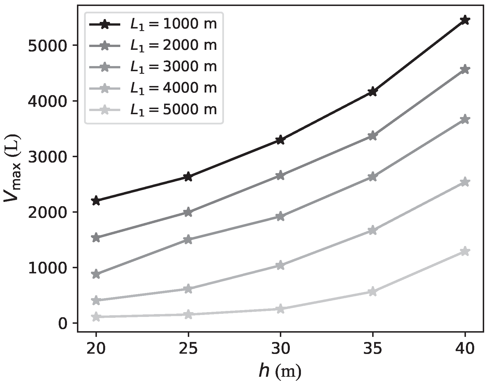
The physical quantities most relevant to the study of extreme transient heads are as follows: pipeline length experiencing negative pressures (), maximum HG in the system (), and mean maximum hydraulic head (). Variations in the following parameters are considered: five values for (1000, 2000, 3000, 4000, and 5000 m), five values for h (20, 25, 30, 35, and 40 m), and 17 values for (ranging from zero to 0.40). Furthermore, the response without air valve protection is also included for comparison.
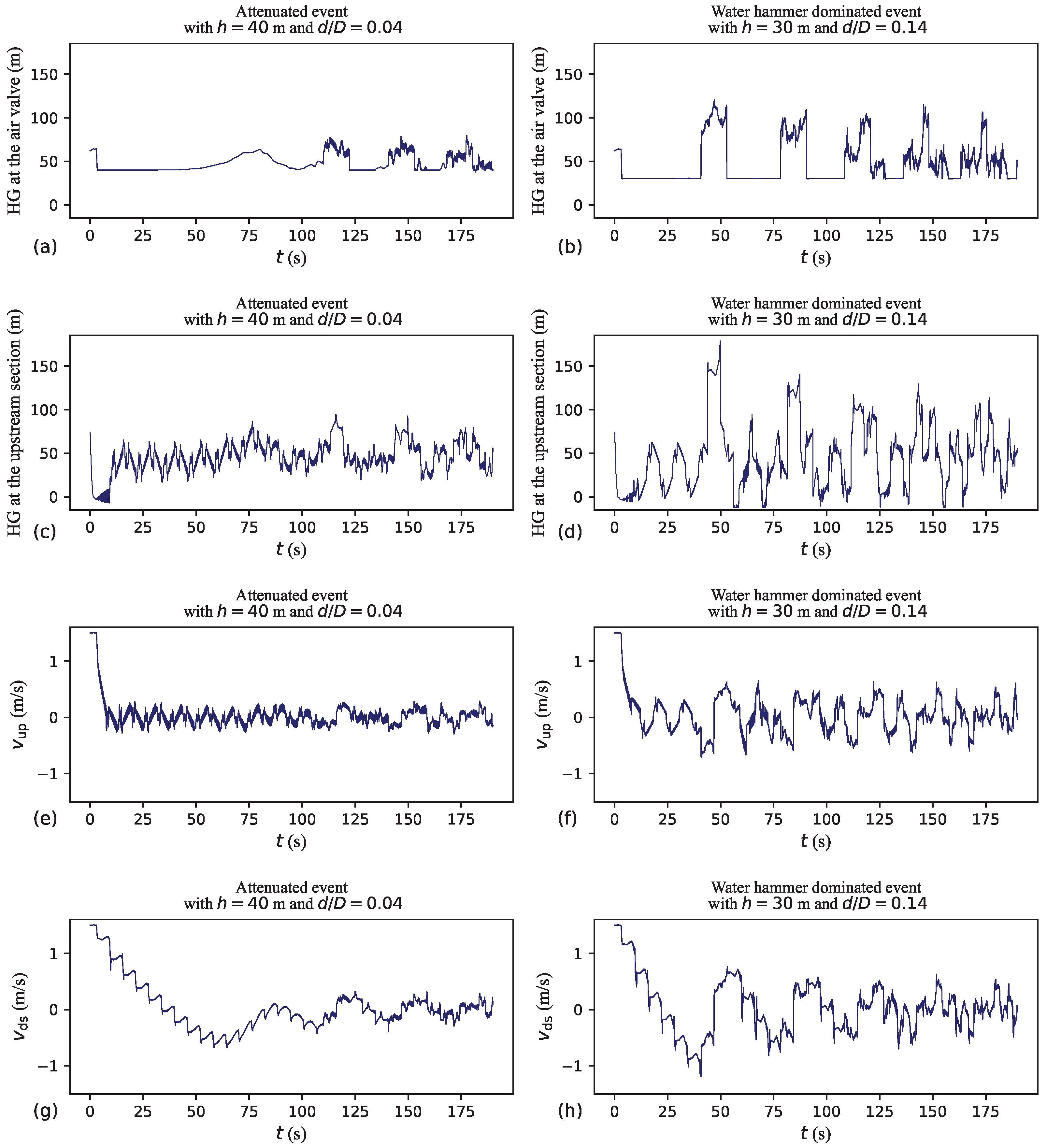
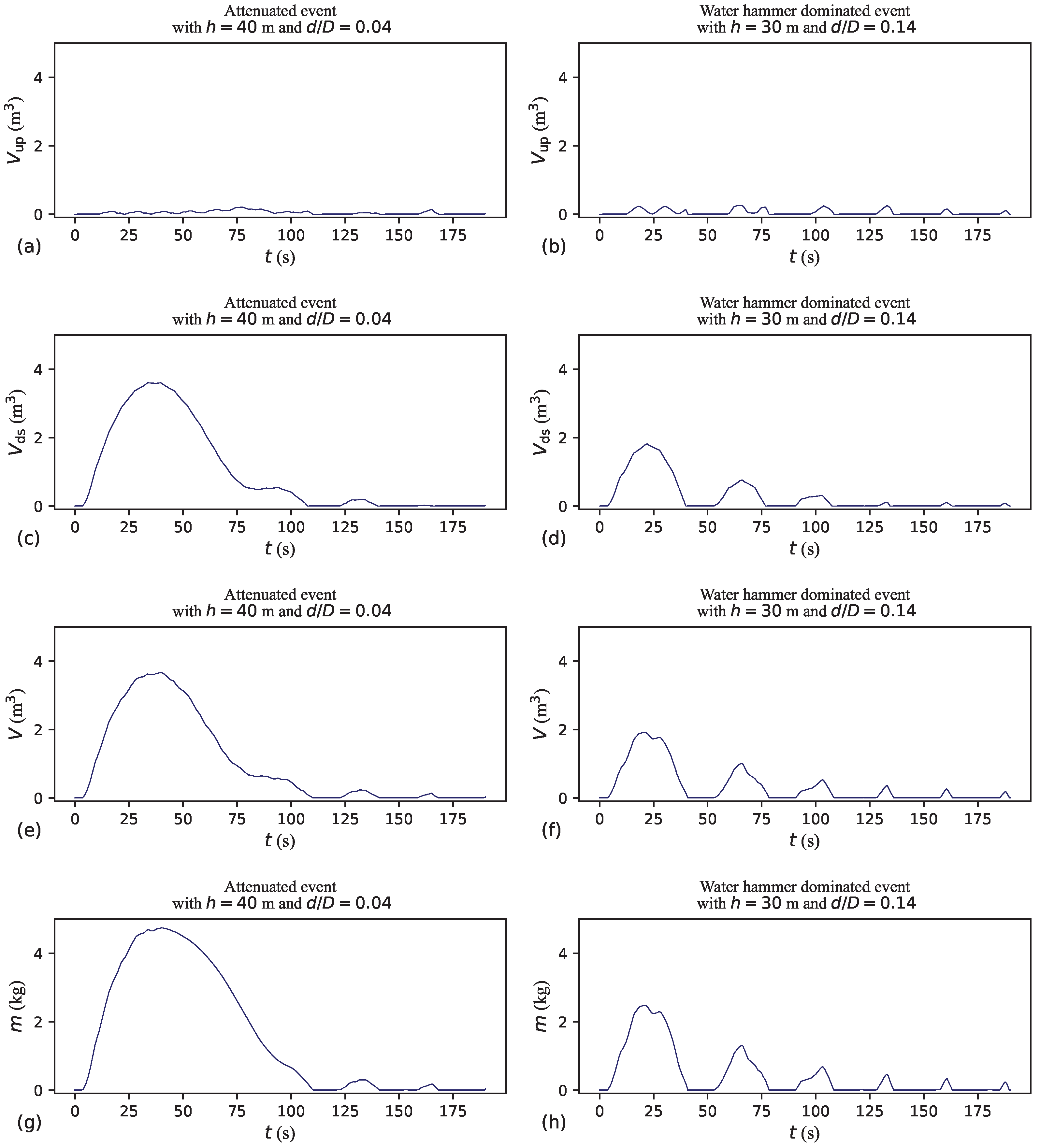
Air valves are typically thought of as devices responsible for mitigating negative pressures. However, as illustrated in
Figure 2 and
Figure 3, even with a system equipped with a large-inflow-capacity air valve, momentary negative pressures can still occur during the pump trip scenario.
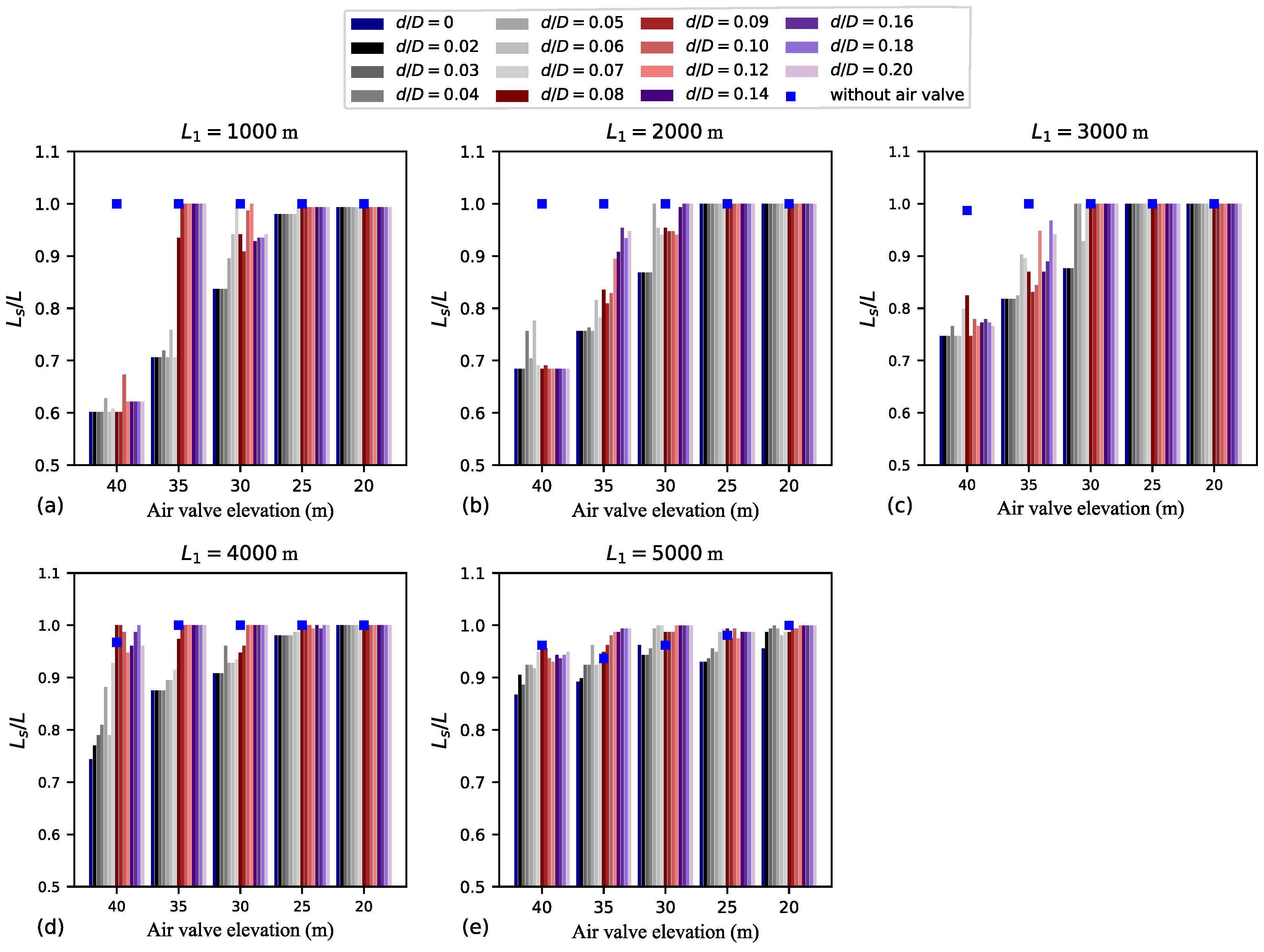
Figure 9 shows how
is influenced by variations in
,
h, and
. Generally, for the smallest
h values (20 and 25 m), negative pressures are prevalent throughout the entire pipeline length, irrespective of
. Particularly for larger
h values, smaller outflow orifices correspond to smaller
values. In fact, the smallest
values are those associated with
m and
m. Interestingly, even for the cases with the smallest
values,
. As exemplified in
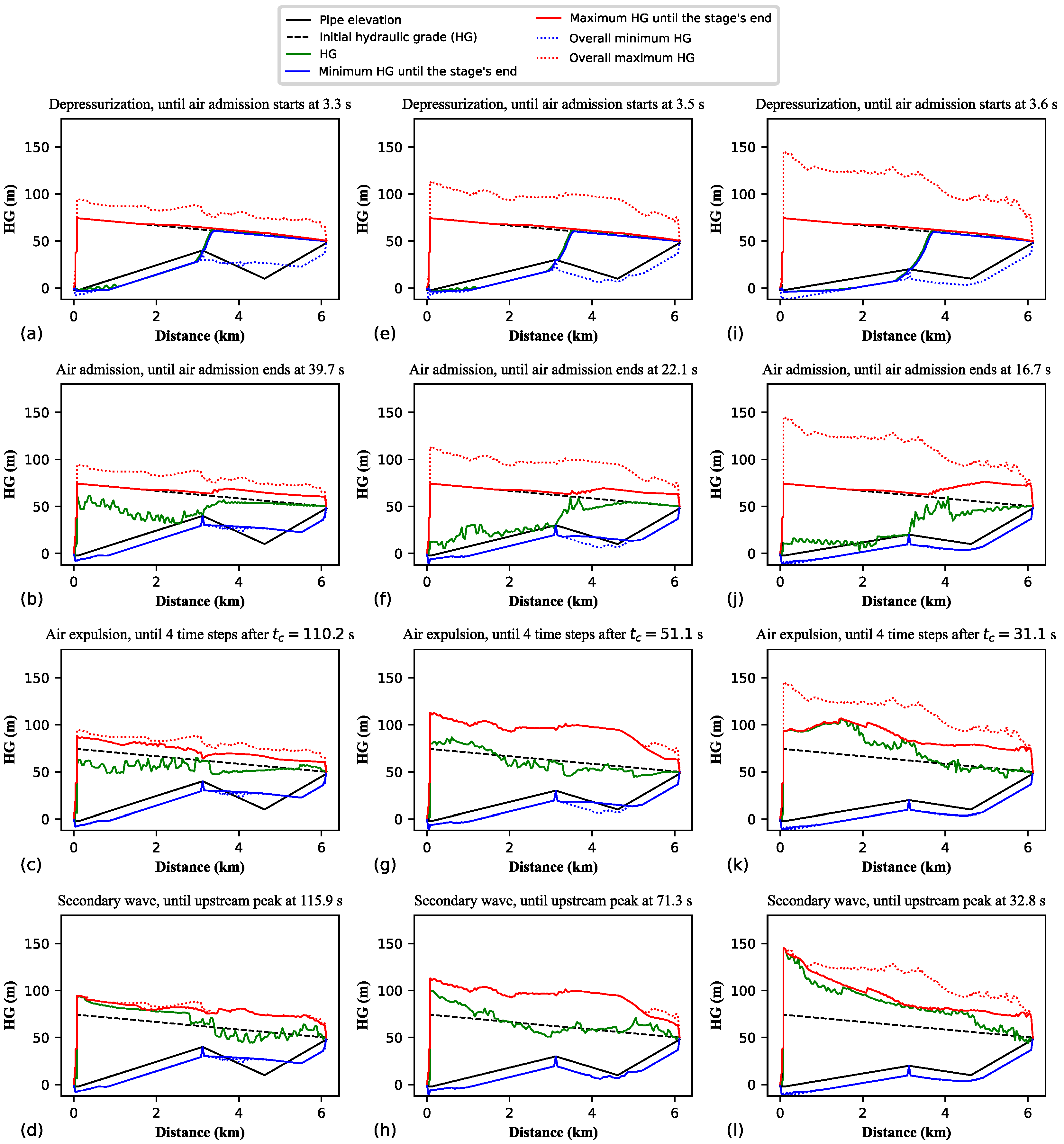
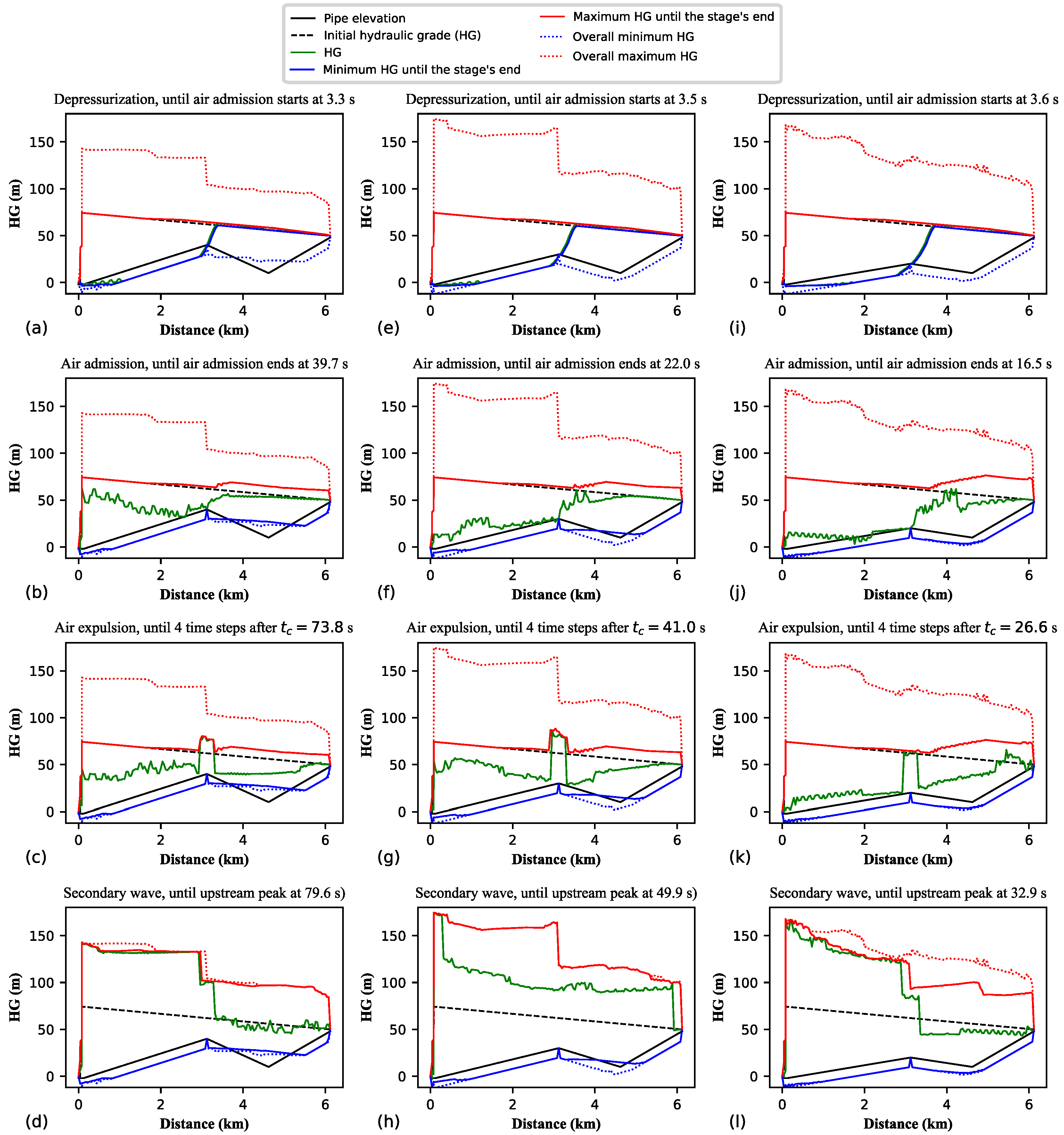
Figure 2a–d and
Figure 3a–d, especially for the largest
h values, the region of the pipeline neighbouring the low point downstream of the air valve is the least susceptible to negative pressures. Nonetheless, in the absence of air valve protection, the whole pipeline is generally subjected to negative pressures.
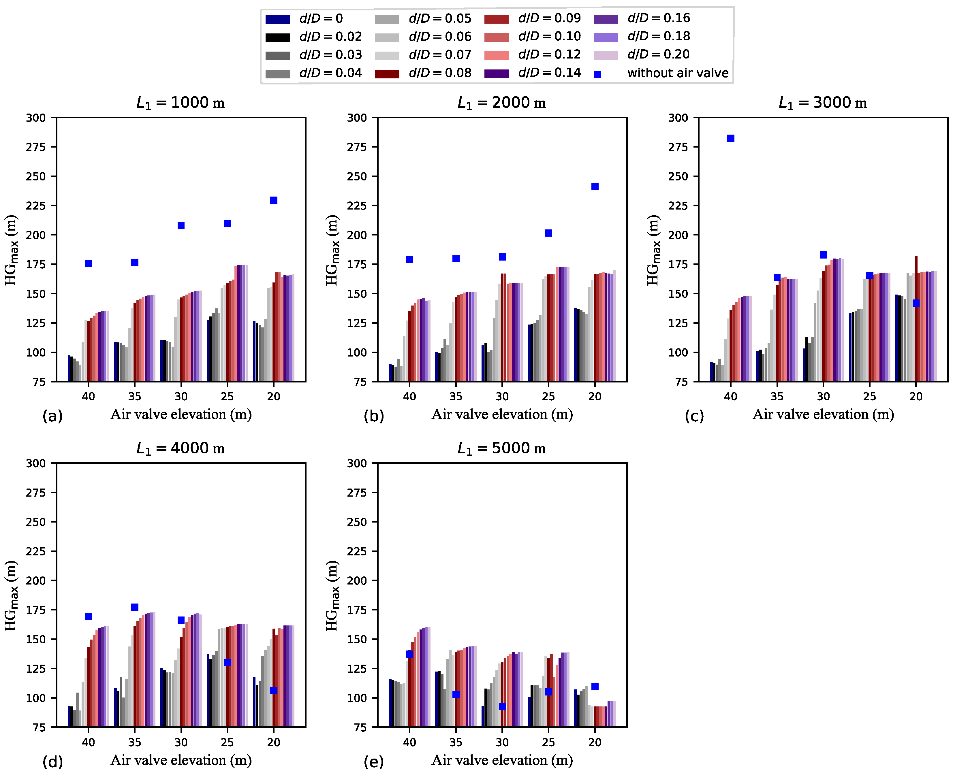
Having an air valve with a sufficiently small outflow orifice can help mitigate the intensity of secondary pressures upon air valve closure. Moreover, as shown in
Figure 10, the presence of an air valve can also help mitigate the maximum transient HG at the upstream section of the pipeline.
Figure 10 shows how
is influenced by variations in
,
h, and
.
Figure 10 reveals that, except for
m and
m (case with the smallest
value), reducing
leads to greater attenuation of
values. For every combination of
and
h (i.e., for every location of the air valve), the
versus
data contains two distinct regions: a lower left region associated with smaller
values (indicating type 1 behaviour), and a higher right region associated with larger
values (indicating type 3 behaviour).
For m and m, with h ranging from 25 to 40 m, the transient magnitude tends to increase as h decreases. Similarly, for m and m, with h ranging from 30 to 40 m, the transient magnitude also tends to increase as h decreases. Interestingly, for the air valve location furthest from the upstream reservoir, the transient magnitude tends to decrease as h decreases. For m and m, is larger for the cases without an air valve than for the cases with it. Pipelines with smaller h values or those located farther from the upstream reservoir are more susceptible to macro-cavitation and tend to have smaller admitted air volumes. As mentioned earlier, the effectiveness of the air valve in reducing the transient magnitude is linked to the air cushioning effect, which is less pronounced in these situations.
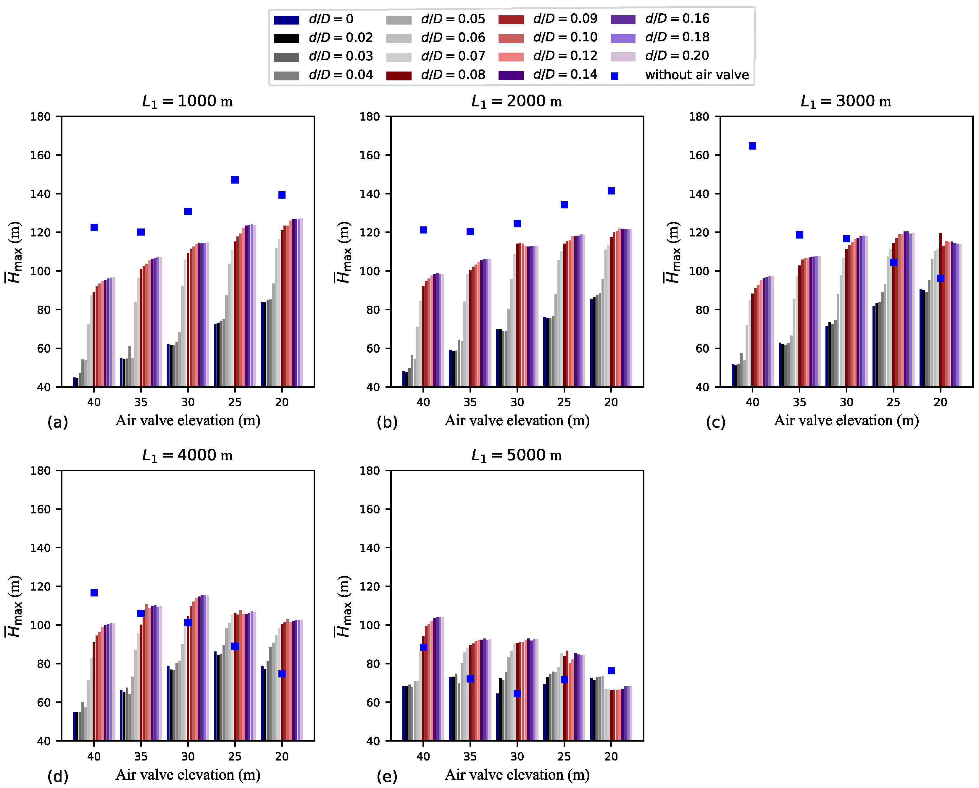
Even though
is an important parameter for evaluating the magnitude of the transient (since the upstream section of the pipeline must withstand the head associated with
), the mean maximum hydraulic head (
) offers a more comprehensive assessment of the entire transient event.
Figure 11 shows how
is influenced by variations in
,
h, and
. The results in
Figure 11 resemble those in
Figure 10. However, the
versus
data in
Figure 11 appear smoother and show more distinct left and right plateaus. It is important to note that if the
ranges considered in
Figure 10 and
Figure 11 were narrower, the presence of the left and right plateaus could shrink or even disappear. The effectiveness of a small-outflow-capacity air valve in mitigating transient events is evident in
Figure 11. For
m and
m,
m for
, whereas
m for
(a 45% difference). For
m and
m,
m for
, whereas
m for
(a 22% difference). It is important to highlight the significance of air valve elevation: e.g., for
m, the water-hammer-dominated event for
m (with a lower driving head to induce reverse flow) displays a transient magnitude similar to that of the attenuated event for
m.
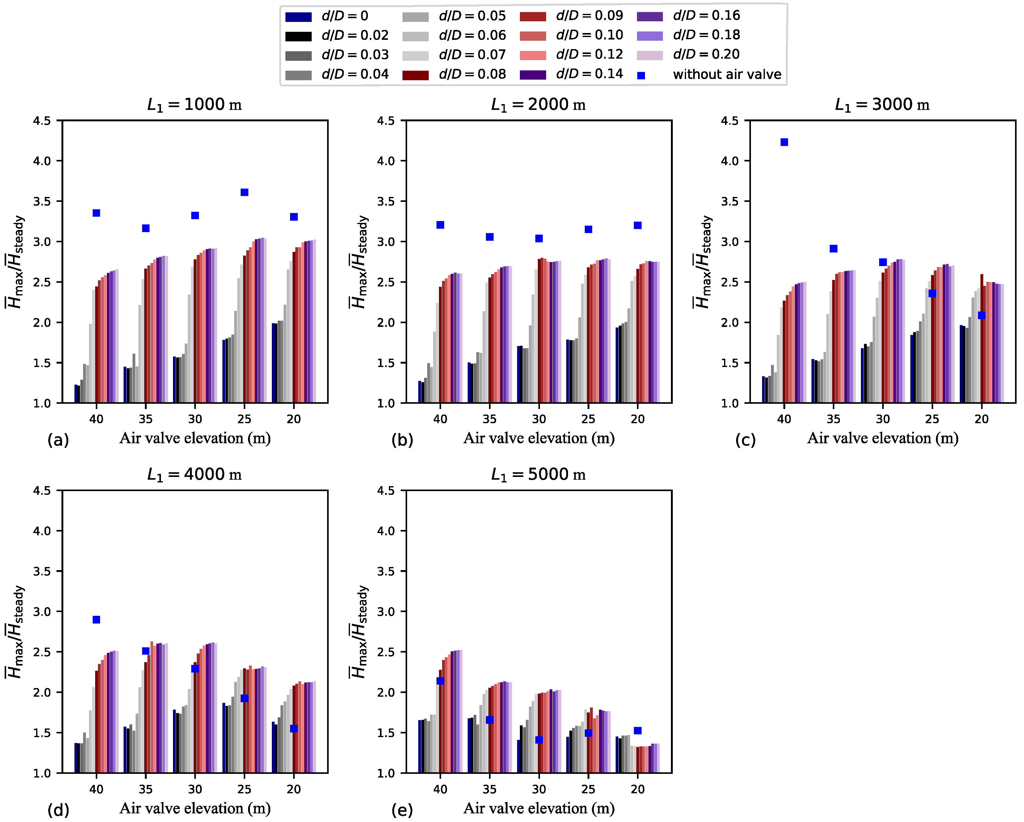
The data shown in
Figure 11 are reinterpreted in
Figure 12 using a dimensionless parameter denoted as
, a parameter that relativises the mean maximum transient head (
) relative to steady values (
). Note that there is a slight variation in the
value depending on the location of the air valve. The highest
value, approximately 3, is observed for
m, the lowest air valve elevations, and type 3 behaviour. In contrast, the smallest
value, approximately 1.2, is observed for
m,
m, and type 1 behaviour. This implies that locating the air valve closer to the upstream reservoir results in more intense transient pressures for type 3 behaviour. However, locating the air valve near the upstream reservoir also offers the greatest potential for water hammer mitigation for type 1 behaviour.
Figure 10,
Figure 11 and
Figure 12 show how the transient magnitude is significantly influenced by the air valve location.
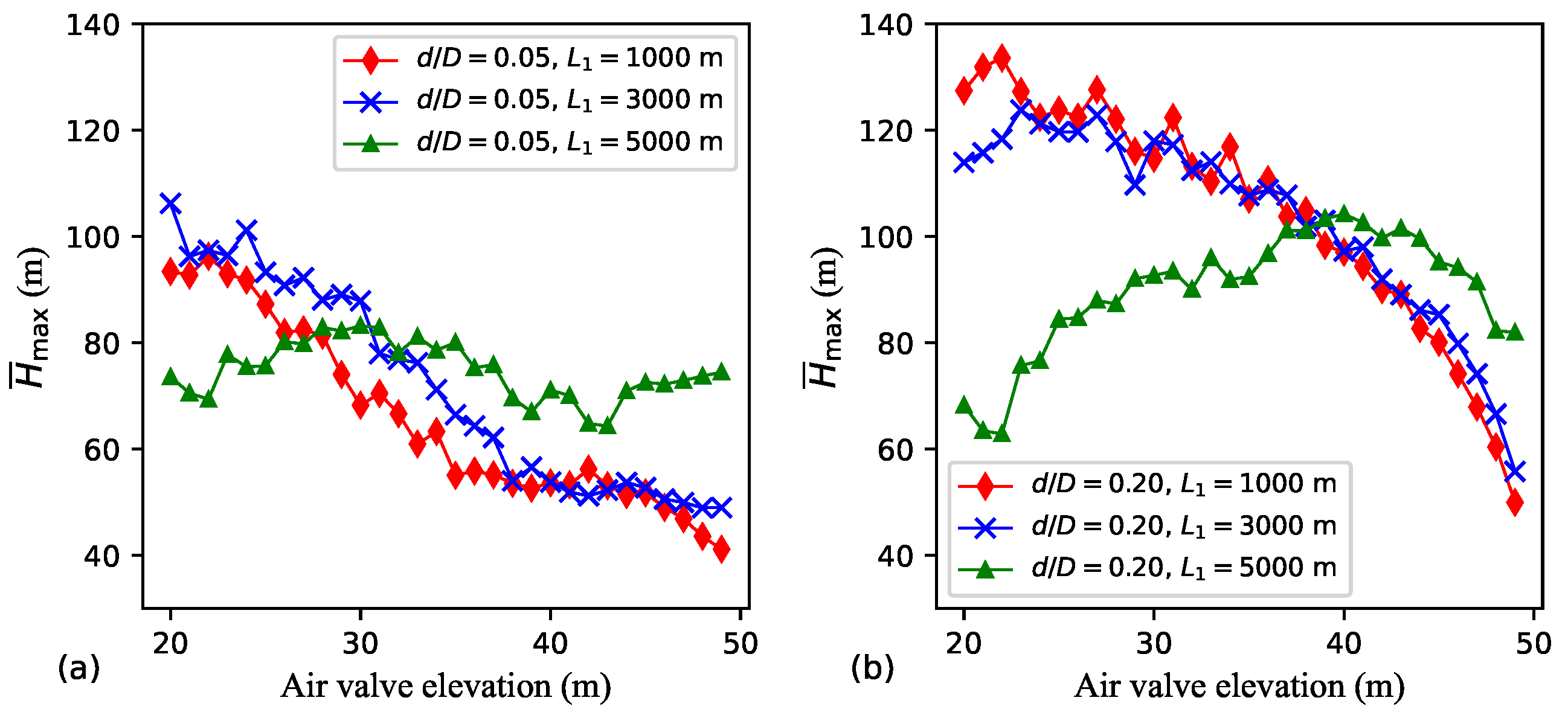
Figure 13 details the effect of
h on
for three
values (1000, 3000, and 5000 m) and two
values (0.05 and 0.20). For both
m and
m,
tends to increase as
h decreases. For
and
m, the dependence between
and
h is unclear, while for
and
m,
shows some tendency to decrease as
h decreases. For each air valve location,
is generally smaller for
than for
.
Figure 13 reveals that, in the context of the pump trip scenario, it is the lower high points that result in more intense transient events.
7.2. Assessing the Timing of the Transient
As previously discussed, the duration of the initial water hammer cycle tends to extend with decreasing values of
and
, as well as increasing values of
h. As illustrated in
Figure 2 and
Figure 3, the initial duration of the water hammer cycle is typically slightly longer than
, making
a suitable proxy for this duration.
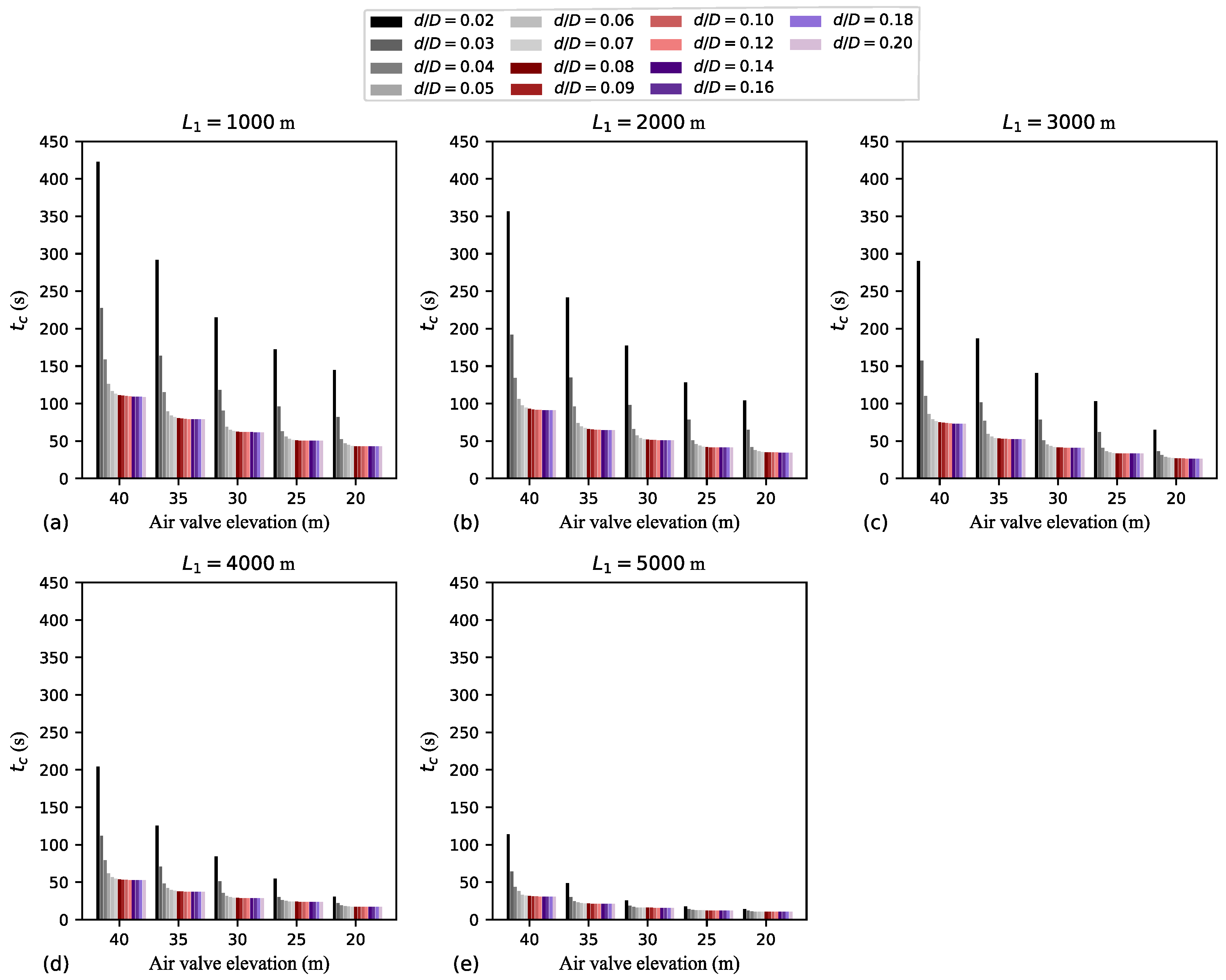
Figure 14 shows how
is influenced by variations in
,
h, and
. In this figure, the case with
was excluded because of the absence of air pocket collapse.
Figure 14 shows that, for each
and
combination, as
h decreases, so does
. For each
h and
combination, as
increases,
decreases. For each air valve location (i.e., for each
and
h combination), as
decreases,
increases exponentially, while as
increases,
tends to a constant value. Indeed, for each air valve location, the largest
value occurs for
. Notably, the
value for a small outflow orifice can be several times longer than that for a large outflow orifice. For
m and
m,
s for
, whereas
s for
(a 74% reduction). For
m and
m,
s for
, whereas
s for
(a 70% reduction). For
m,
is much smaller than for
m. For example, for
m,
m, and
(type 1 behaviour),
s—a value much smaller than that for type 3 behaviour considering
m,
m, and
(
s). A combined examination of
Figure 11 and
Figure 14 reveals a consistent trend: event intensity attenuates with increasing
, as momentum considerations would indicate.
An essential aspect regarding transient timing is the moment when the maximum hydraulic grade in the system (
) occurs. The moment when
occurs is referred to as
. As discussed, a peak HG value occurs at the upstream section of the pipeline after the first instance of air pocket collapse. Yet, this peak HG does not always correspond to
. In
Figure 3, for example, the peak HG values at the upstream section of the pipeline at the conclusion of the secondary wave stage correspond to the
values. However, since such correspondence is not always the case, one method to assess the timing of the maximum HG in the system is by comparing it to the air pocket collapse time.
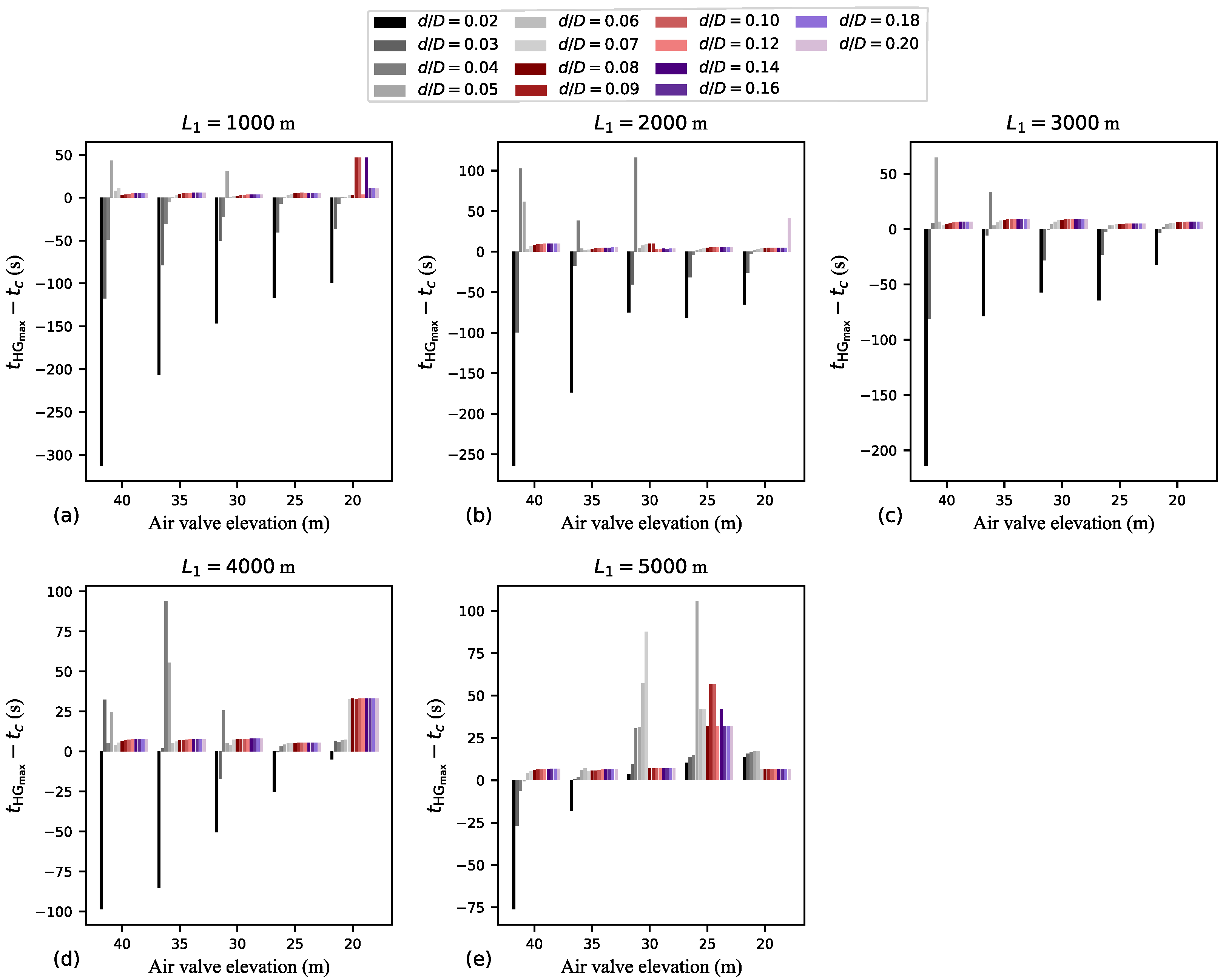
Figure 15 shows how
minus
is influenced by variations in
,
h, and
. A negative bar in this figure indicates that
occurs before
, whereas a positive bar indicates the opposite.
In
Figure 15, three distinct
patterns can be identified, which are somewhat dependent on the air valve location and outflow capacity: (i)
occurs much before
(typical for small
values); (ii)
occurs much after
(sometimes observed for intermediate
values); (iii)
occurs right after
(typical for large
values). For
m (especially for lower
h values like 20, 25, and 30 m), the
patterns become less distinct compared to other
values. For the smallest
values,
occurs much before
, while for the largest
values,
usually occurs right after
. In the context of type 3 behaviour, the usually relatively small and positive value of
for large
values reinforces the connection between air valve closure and the occurrence of
. However, for intermediate
values,
can be several times the pipeline’s period.
The striking difference in transient timing between type 1 and type 3 behaviours is evident in
Figure 15. For
m and
m,
s for
(which is actually a non-extreme case), which is a value comparatively much larger in absolute magnitude than
s for
. In
Figure 15, the number of
cases with negative
values decreases as
increases or
h decreases. Negative
values indicate that
occurs while the air pocket remains. Thus, in such cases, it makes sense to infer that
is associated with the air expulsion stage, i.e.,
occurs while the air pocket is being compressed by the reverse flow in the downstream branch. The transient timings associated with type 1 and type 2 behaviours occurring well before or much after
, respectively, do not necessarily rule out the possibility of a peak transient head occurring at the upstream section of the pipeline immediately after the air valve closure.
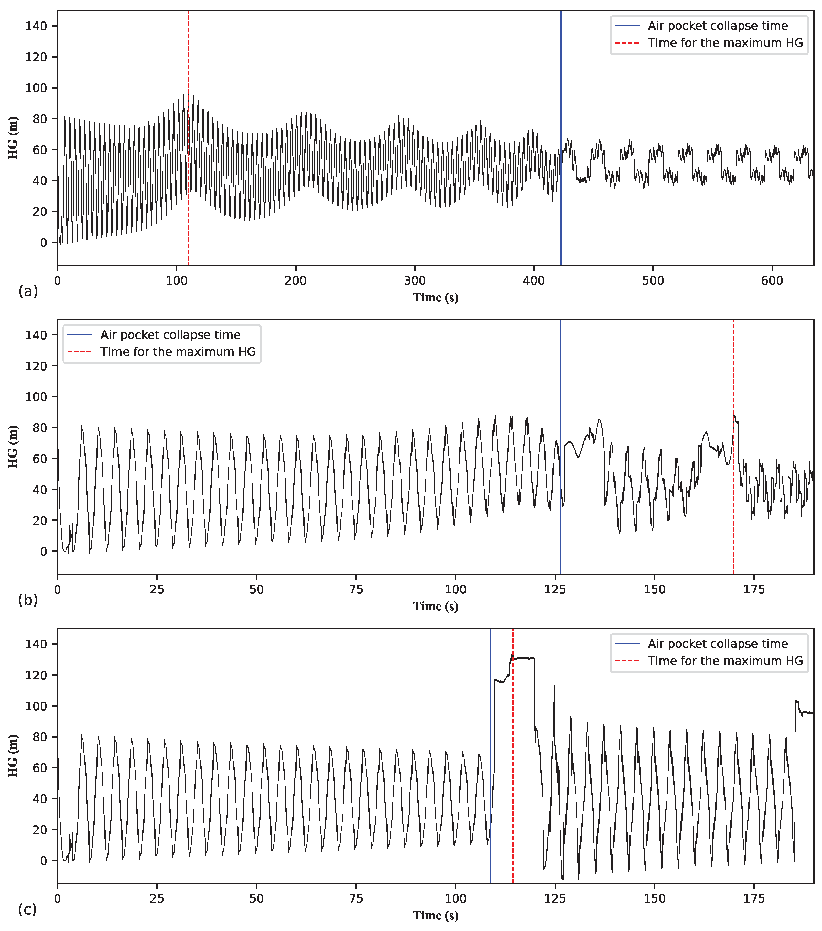
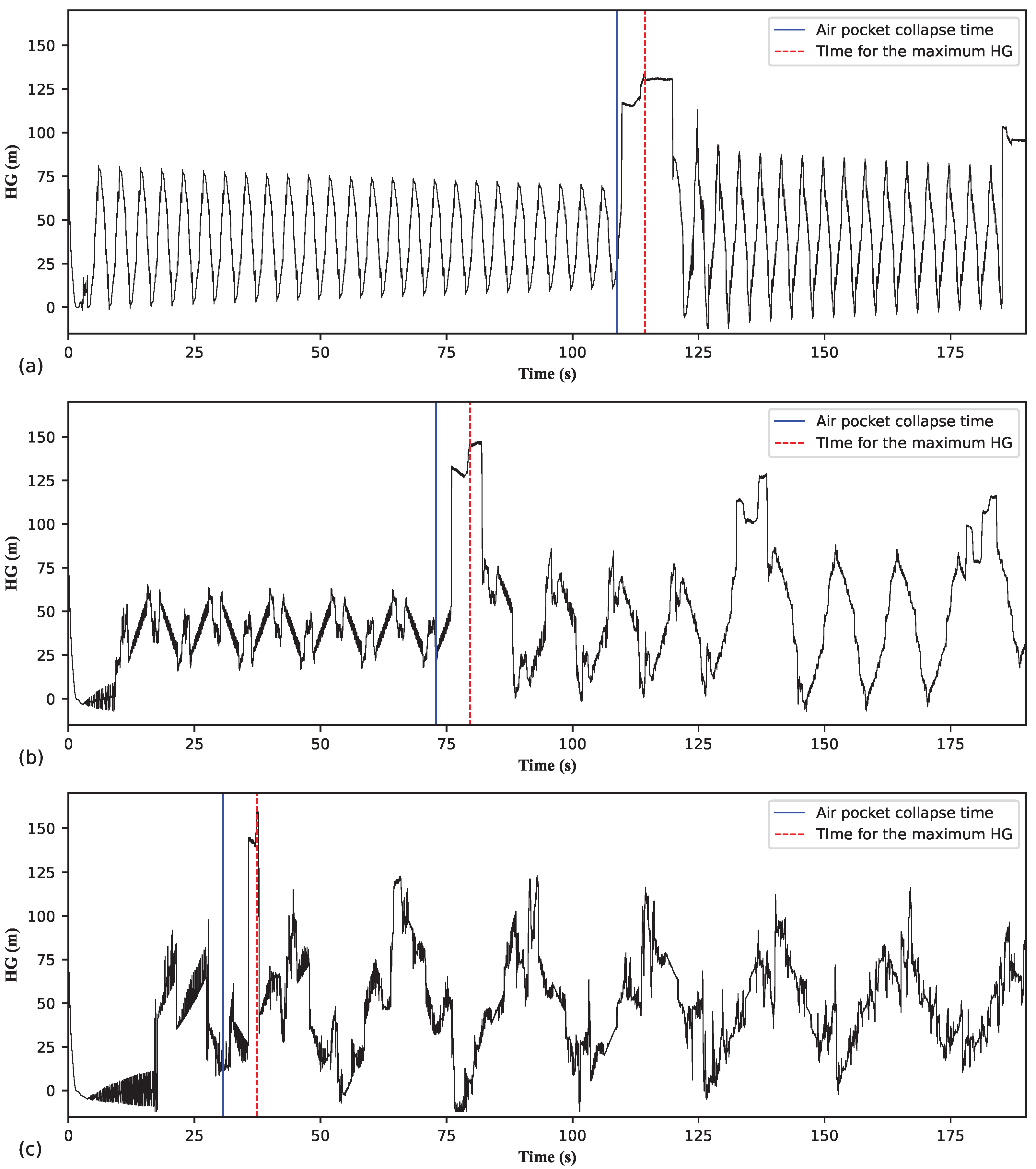
Figure 16 shows the evolution of the HG at the upstream section of the pipeline (i.e., close to the pumping station) for types 1, 2, and 3 behaviours. For
(
Figure 16a),
occurs much before
. For this case,
is about four times longer than
. For
(
Figure 16b),
is considerably longer than
. For this case,
occurs after the second instance of air pocket collapse. In
Figure 16b, note the similarity in the HG signal right after
and right before
. This kind of HG variation is typical of the secondary wave stage. Also, note that in
Figure 16b, the magnitude of the HG peak right after
is similar to the magnitude of
. For
(
Figure 16c),
occurs right after
. In general, in
Figure 16, prior to
, the transient variations share the same frequency across all three cases.
Figure 17 shows the evolution of the HG at the upstream section of the pipeline for three examples of type 1 behaviour (i.e., for three
values) considering
m and
. Across all three cases,
. Prior to
, the frequency of the transient oscillations decreases as
increases. The time it takes for the transient wave to traverse the upstream branch is directly proportional to
. The absolute value of
decreases as
increases. Unlike the wave pattern depicted in
Figure 16b,c, the HG oscillation in
Figure 17 is not momentarily disrupted after the collapse of the air pocket. Following
, the oscillation period stabilises at
for all three
cases in the figure. For
m, with its relatively short
value, it becomes somewhat difficult to discern the period of the HG oscillation before
. In
Figure 17a,b, the oscillation period before
is determined by
(as predicted by Ramezani and Karney (2017) [
10]), resulting in 4 s for
m and 12 s for
m.
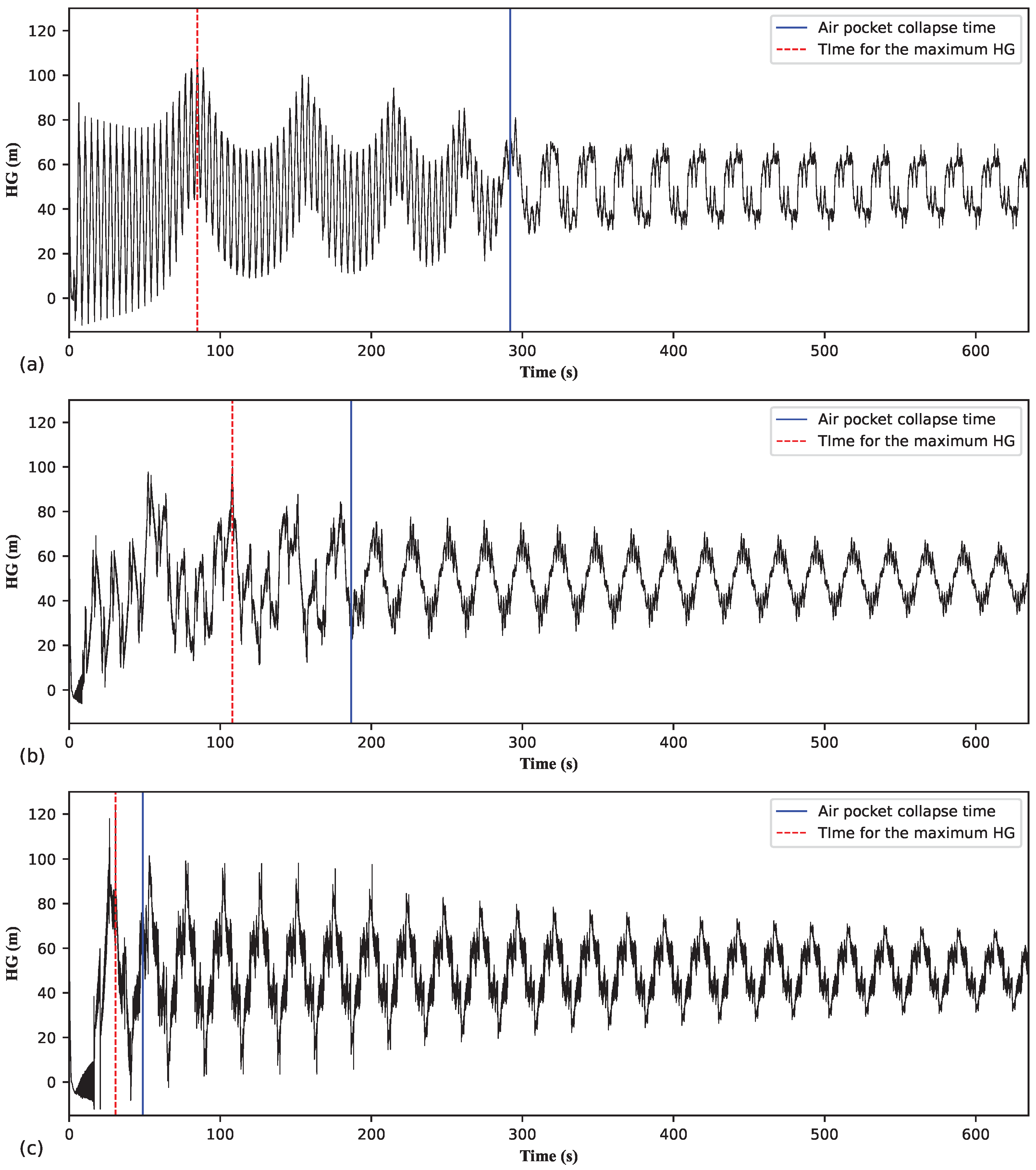
Figure 18 shows the evolution of the HG at the upstream section of the pipeline for three examples of type 3 behaviour (i.e., for three
values) considering
m and
. Across all three cases,
. In contrast to
Figure 17, in
Figure 18, the
values across all three cases are similar. The frequency of the transient oscillations decreases as
increases. Notably, the frequency of the oscillations remains the same both before and after the collapse of the air pocket. This behaviour pattern arises from the multiple instances of air admission and expulsion characteristic of type 3 behaviour, as shown in
Figure 18, in contrast to the type 1 behaviour shown in
Figure 17. This observation aligns with the data presented in
Figure 7. The frequency of the transient oscillations in
Figure 18 is determined by
. In contrast to
Figure 17, in
Figure 18, the secondary wave stage can be easily discerned as a discontinuity in the HG oscillations. In
Figure 18b, three instances of secondary wave stages can be observed, each showing progressively attenuated associated HG peaks.
7.3. Representing the Sensitivity Data
The air exchange apertures commonly examined in the literature are orifices and air valves. It is important to highlight the distinction in pipeline transient behaviour between these apertures. For the filling procedure in a pipeline with a downstream orifice, the absolute maximum transient head (often referred to as
) increases with increasing
until the maximum
value is reached. Then,
starts to decrease as
increases. The
value associated with the maximum
value is referred to as the critical
value. The pipeline transient behaviour associated with the occurrence of the maximum
value can be classified as water-hammer-dominated and is characterised by a sudden increase in head resulting from the impact of the filling water column against the downstream orifice. References providing data on the transient magnitude versus
for the pipeline filling procedure involving a downstream orifice include Zhou et al. (2002) [
37], Lee (2005) [
38], Zhou et al. (2019) [
39], and Zhou et al. (2020) [
3].
When filling a line with a downstream orifice, the orifice initially vents air to accommodate the incoming water. Nonetheless, as the water front reaches the orifice and in the subsequent moments, the orifice might expel not only air but also a mixture of air and water. In contrast, when filling involves a downstream air valve, only air is expected to be discharged. Even in cases where there might be a delay in air valve closure or if the last portion of the exhausted air contains moisture, the release of water or a mixture of air and water through the air valve is only momentary. Since air valves are designed to close upon contact with liquid water, the transient magnitude is anticipated to stabilise for large values (i.e., to remain the same for values for which the air cushioning effect is negligible). In fact, the air expulsion stage during the pump trip scenario represents a variation of the filling scenario, albeit within a more complex transient event. Notably, the transient magnitude during the pump trip scenario is directly influenced by the extent of the air cushioning effect during the air expulsion stage. As a result, both the pump trip and the pipeline filling scenarios share significant similarities, permitting a comparison between the physical processes involved in both situations.
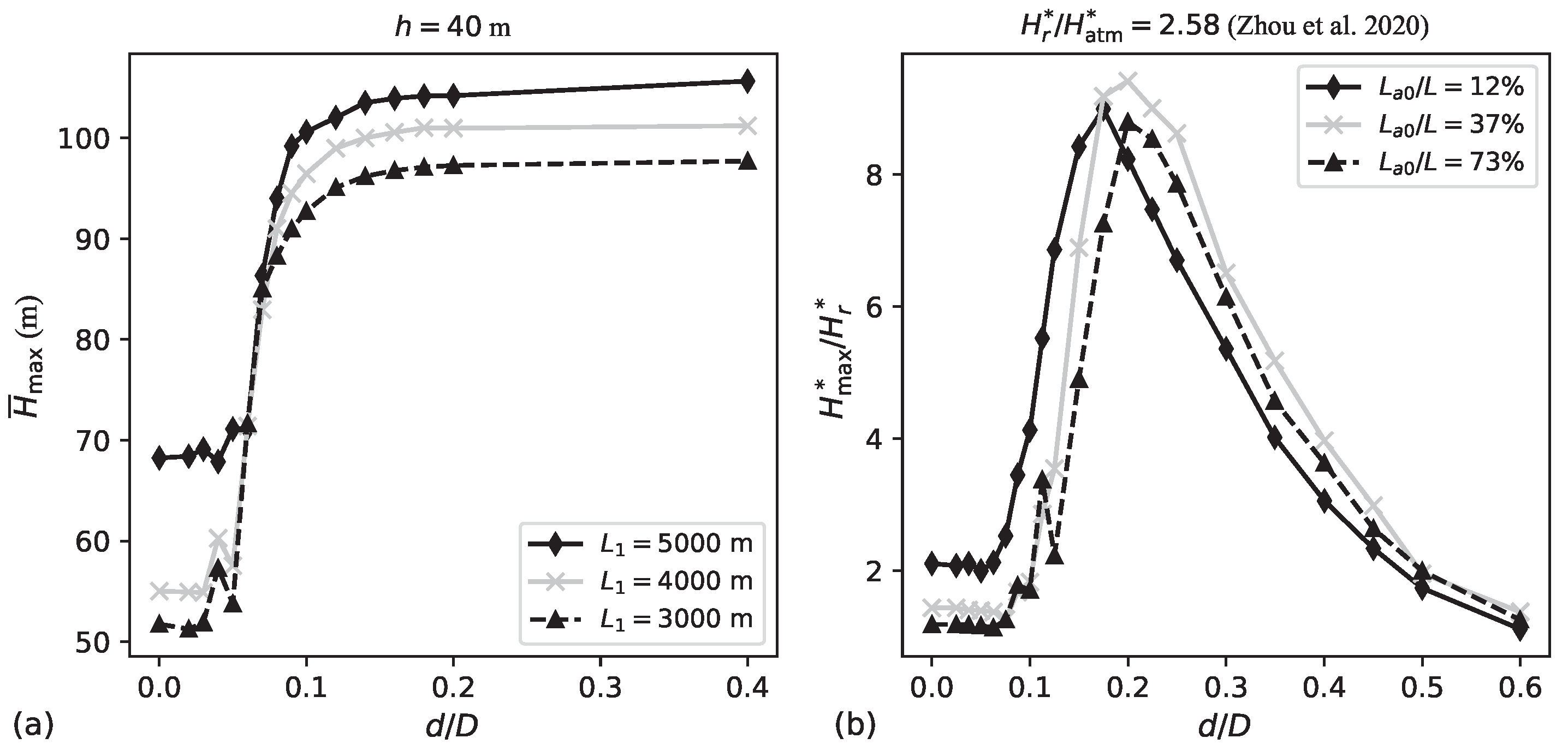
Figure 19 allows a comparison between the transient responses associated with a pump trip and pipeline filling. Specifically,
Figure 19a shows the relationship between
and
for the pump trip scenario involving air exchanges through an air valve.
Figure 19b shows the relationship between
(ratio between the absolute maximum transient head and the absolute inlet head) and
for the pipeline filling scenario involving air exchanges through a simple orifice. In
Figure 19a,b, a strong similarity in transient response is evident between the two cases for small
values. In both cases, if there is an increase in the maximum air pocket volume (achieved, for example, by decreasing
in the pump trip scenario) or the initial air pocket volume, the intensity of the transient event decreases for
values consistent with type 1 behaviour. However, a significant difference in transient response arises if the
values are large.
The critical aperture size for type 3 behaviour (referred to as
) determines the threshold
value above which the transient can be classified as water-hammer-dominated. For the pump trip scenario,
is defined here as the
value above which the transient magnitude stabilises. For the filling procedure,
is defined here as the
value associated with the maximum transient magnitude. On the other hand, the critical aperture size for type 1 behaviour (referred to as
) determines the
value below which the transient can be classified as attenuated.
Figure 19 compares pump trip (
Figure 19a) to filling (
Figure 19b), showing that the transient magnitude curves experience a sharp incline immediately after the low left plateau. However, for small
values prior to this incline, the transient magnitude is relatively constant. The general shape of the curves in
Figure 19a resembles that of a logistic curve. Each of these curves features a lower plateau to the left, followed by a steep (transitional) incline, ultimately reaching a higher plateau to the right. On the other hand, the general shape of the curves in
Figure 19b resembles that of a right-skewed probability density function. Each of these curves features a lower plateau to the left, followed by a steep incline that reaches a maximum point, with a subsequent gradual descent.
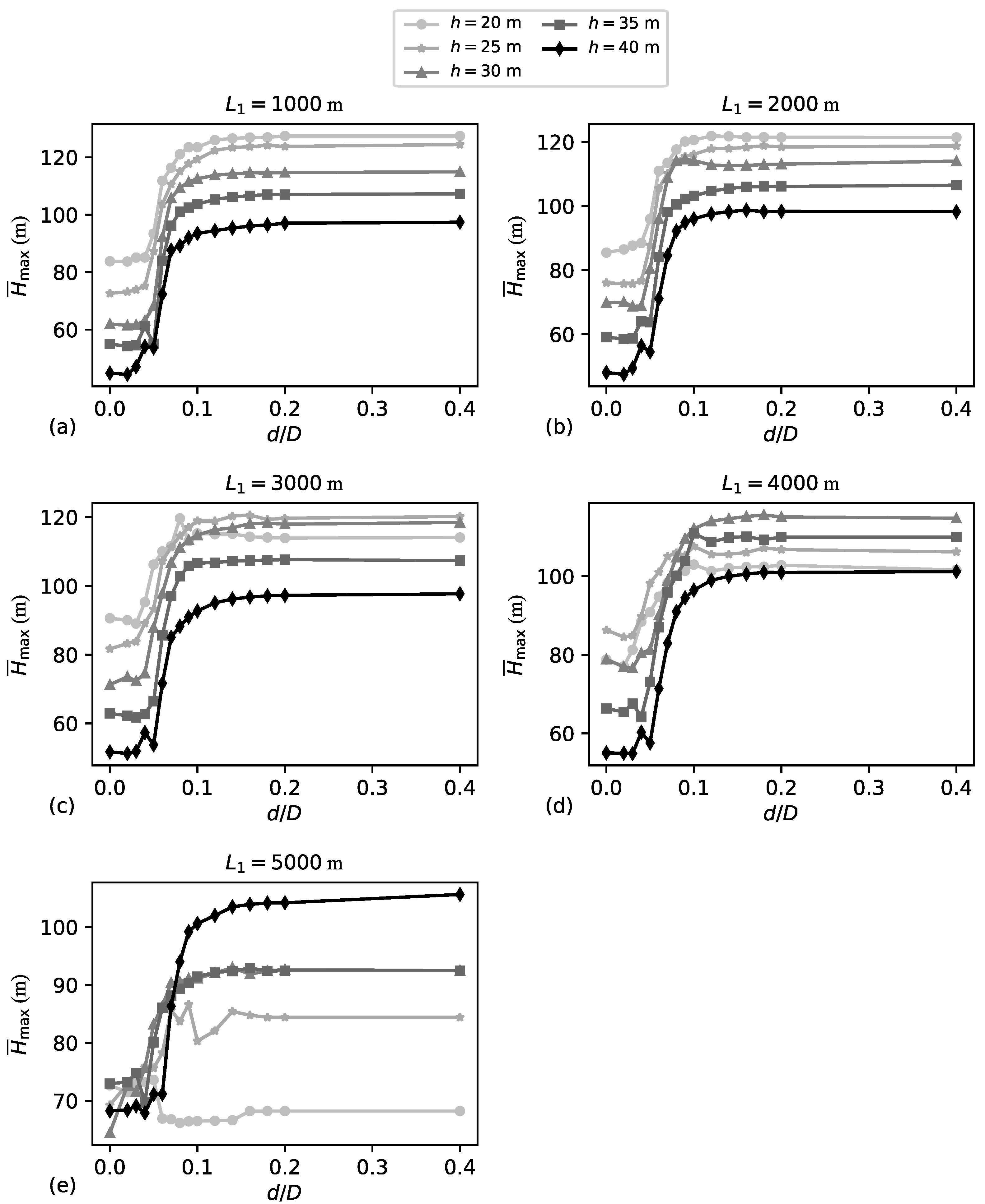
Figure 20 shows the comprehensive
versus
results obtained from the main set of numerical simulations. The curves in
Figure 20 exhibit a similar shape to those in
Figure 19a, except for the case with
m and
m, which is associated with the smallest
value. As mentioned, this distinctive shape resembles the shape of a logistic curve. In
Figure 20, for both
m and
m, regardless of whether it is type 1 or type 3 behaviour, the transient magnitude increases as
h decreases. For
values ranging from 1000 to 4000 m, this trend remains relatively consistent, particularly with respect to the low left plateaus. With the exception of
m, scenarios with
m consistently exhibit the mildest transient magnitudes for both type 1 and type 3 behaviours across different
values.
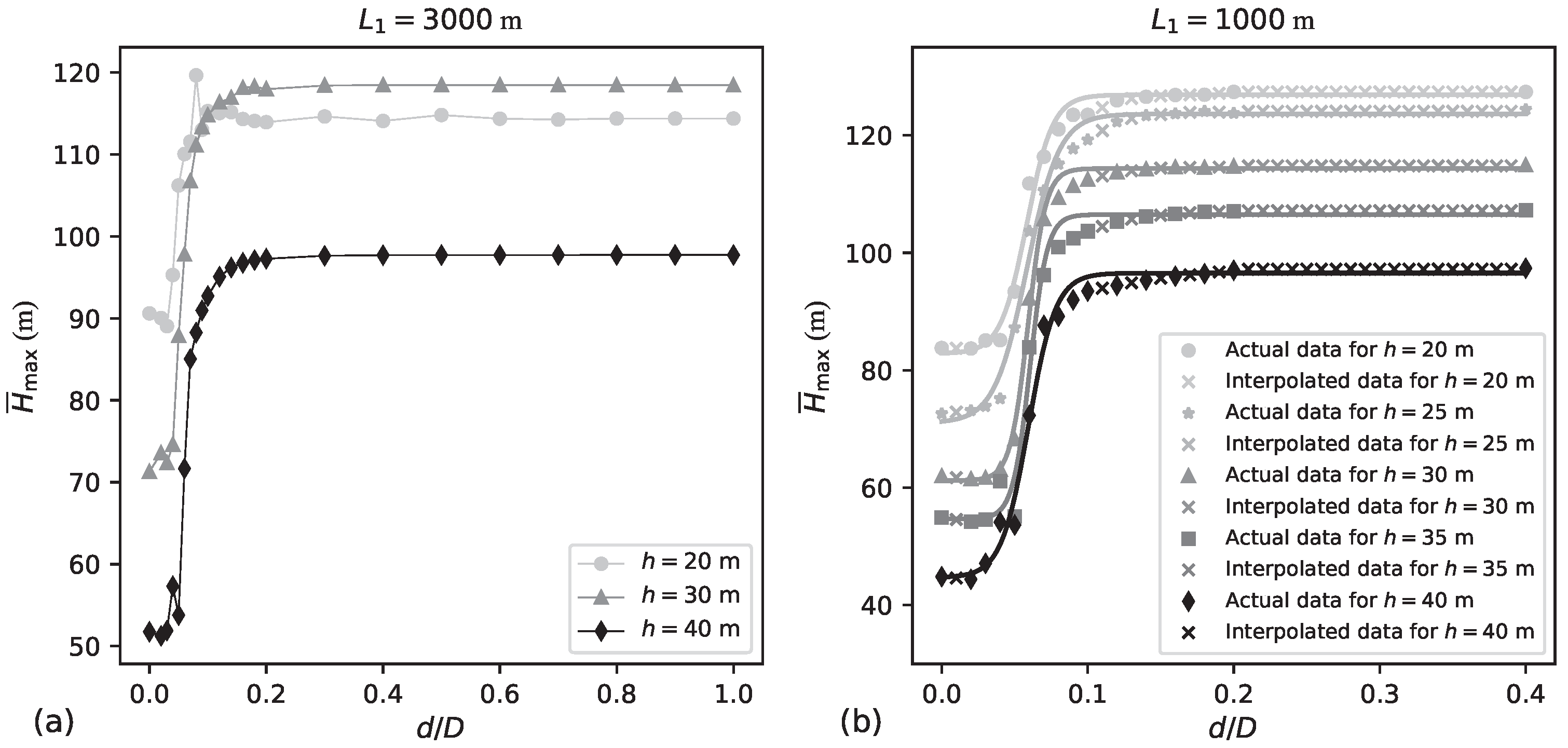
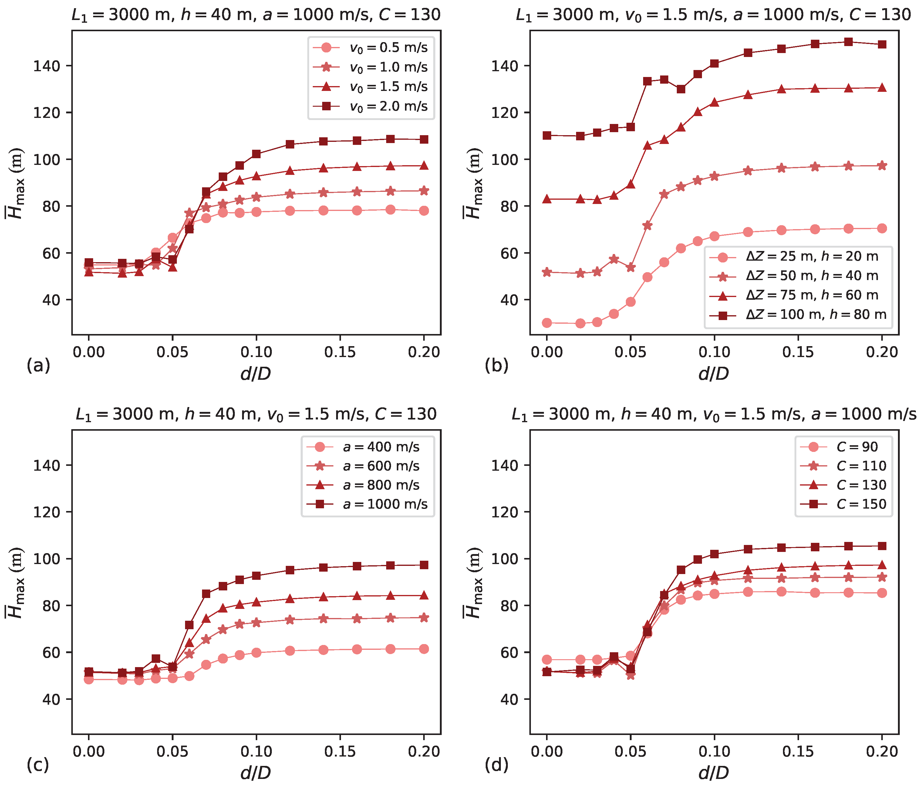
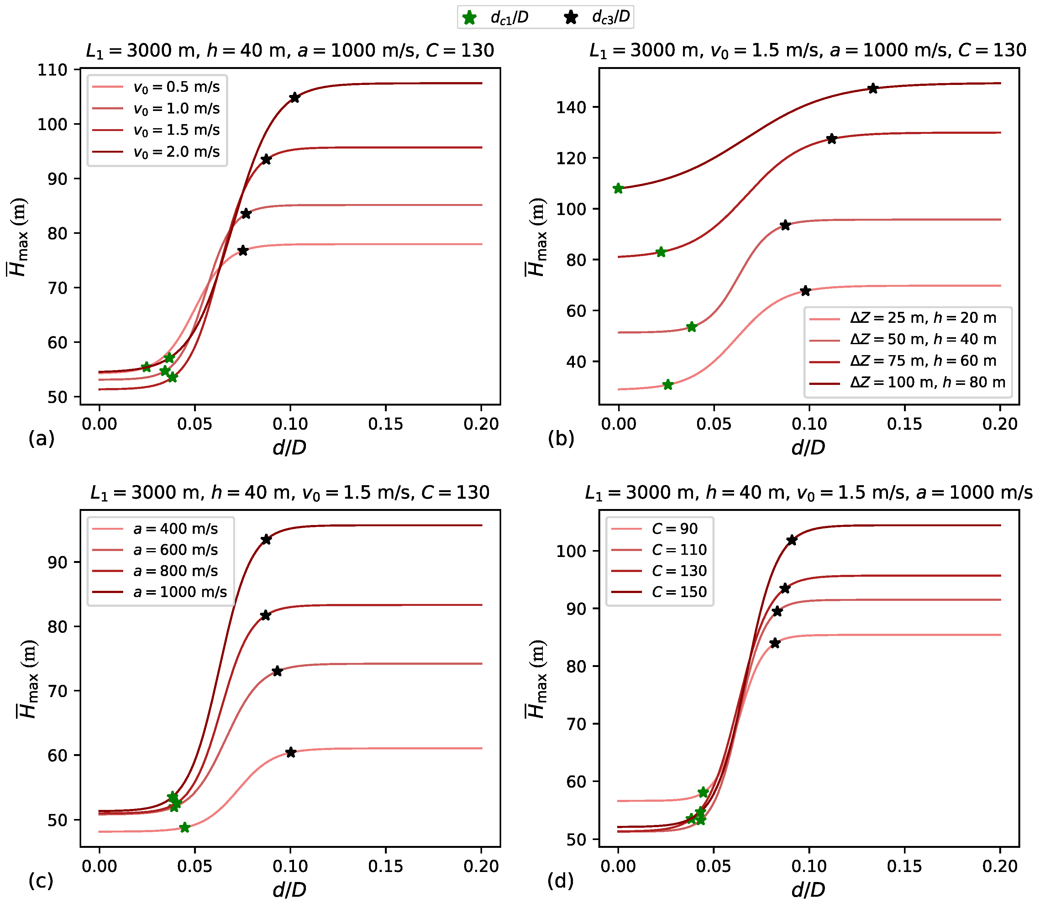
Figure 21 validates the appropriateness of fitting logistic curves to the
versus
results. In
Figure 21a,
remains relatively constant for large
values. In this figure, the length of the high right plateau is significantly longer than that of the low left plateau. In fact, a significant part of the
range in
Figure 21a, specifically the largest
values, is of limited relevance for sizing. Air valves with
values exceeding 0.20 are typically not considered in practice. In
Figure 21b, interpolated data is incorporated into the actual
versus
results to establish an evenly spaced set of
versus
pairs. These interpolated values are considered in the curve fitting process. The fitted curves shown in
Figure 21b have the ability to predict the transient magnitude for both type 1 and type 3 behaviours.
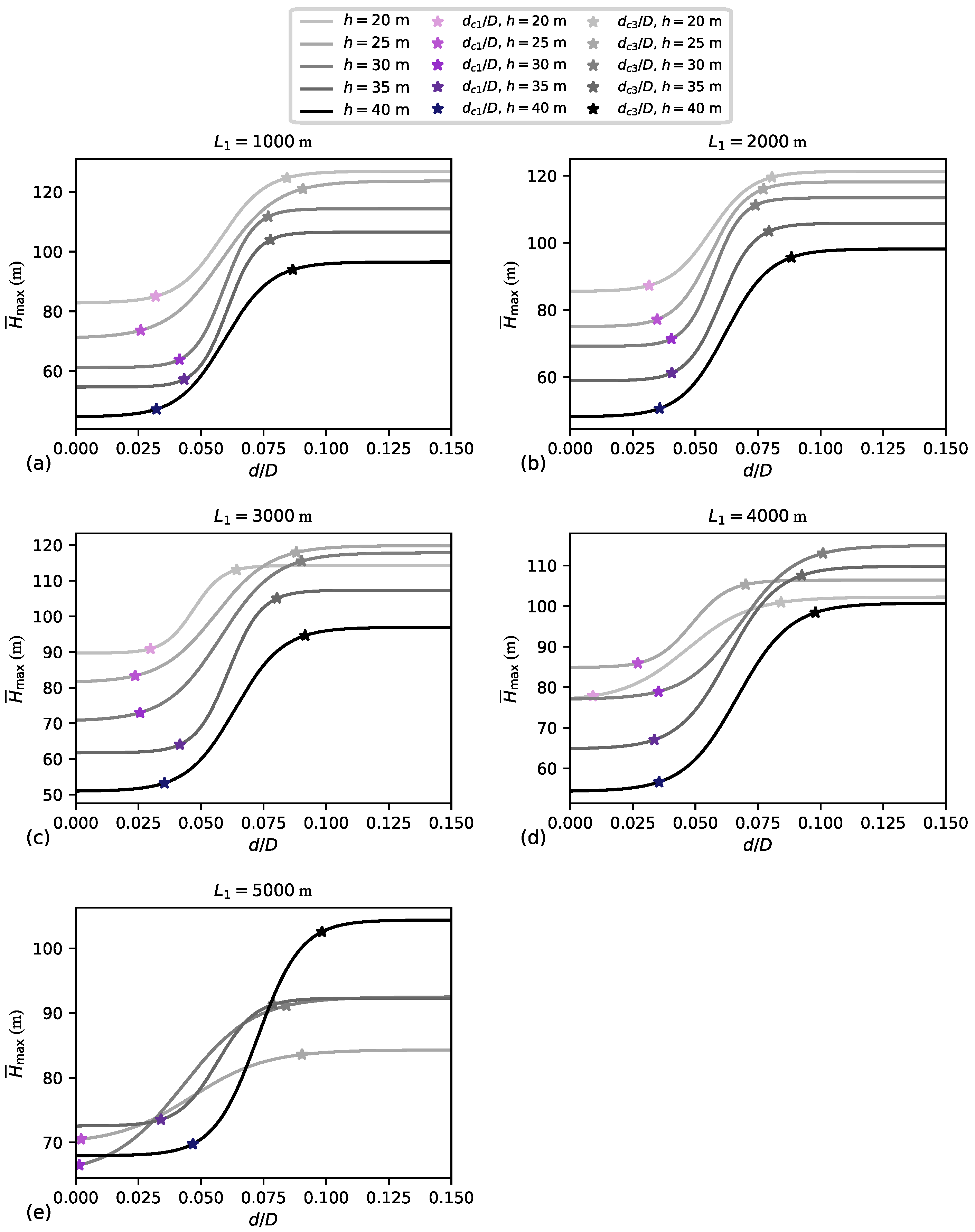
Figure 22 shows logistic curves fitted to the dataset shown in
Figure 20. In
Figure 22, two points along each curve are emphasised: (
,
), which delimits type 1 behaviour; and (
,
), which delimits type 3 behaviour. The
value is determined as the
value corresponding to the minimum
plus 5% of the logistic curve’s height, while
is determined as the
value corresponding to the maximum
minus 5% of the logistic curve’s height. These definitions for the critical air valve orifice sizes, while simple, effectively capture the transitions between the transient behaviours. Using logistic curves instead of raw data enhances the ease of comparing various scenarios and determining the critical orifice sizes.
Table 1 summarises the
and
values for all the cases considered in the main set of simulations, as shown in
Figure 22. Significant variation is found in both the
and
values, depending on the specific combination of
and
h. For example, for the range of
h values considered in this paper, for
m, the range of
spans from 0.024 to 0.042, while the range of
spans from 0.064 to 0.092. To provide greater context, consider the
ranges, which define type 1 behaviour, and the
ranges, which define type 3 behaviour, based on the data reported in Zhou et al. (2019) [
39] for vertical pipe filling and in Zhou et al. (2020) [
3] for horizontal pipe filling with
(ratio between the absolute inlet head and the absolute atmospheric head). When filling a line with a downstream orifice, the transient magnitude versus
data has a low left plateau for type 1 behaviour, but there is no high right plateau for type 3 behaviour, as shown in
Figure 19. In a manner similar to the approach used in
Figure 22 to define
, for pipeline filling with a downstream orifice, the value of
is the
value associated with the transient magnitude determined by adding 5% of the difference between the maximum value of the curve and the value of the low left plateau to the value of the low left plateau itself. Additionally, for this case, the value of
is the
value associated with the maximum on the transient magnitude versus
curve.
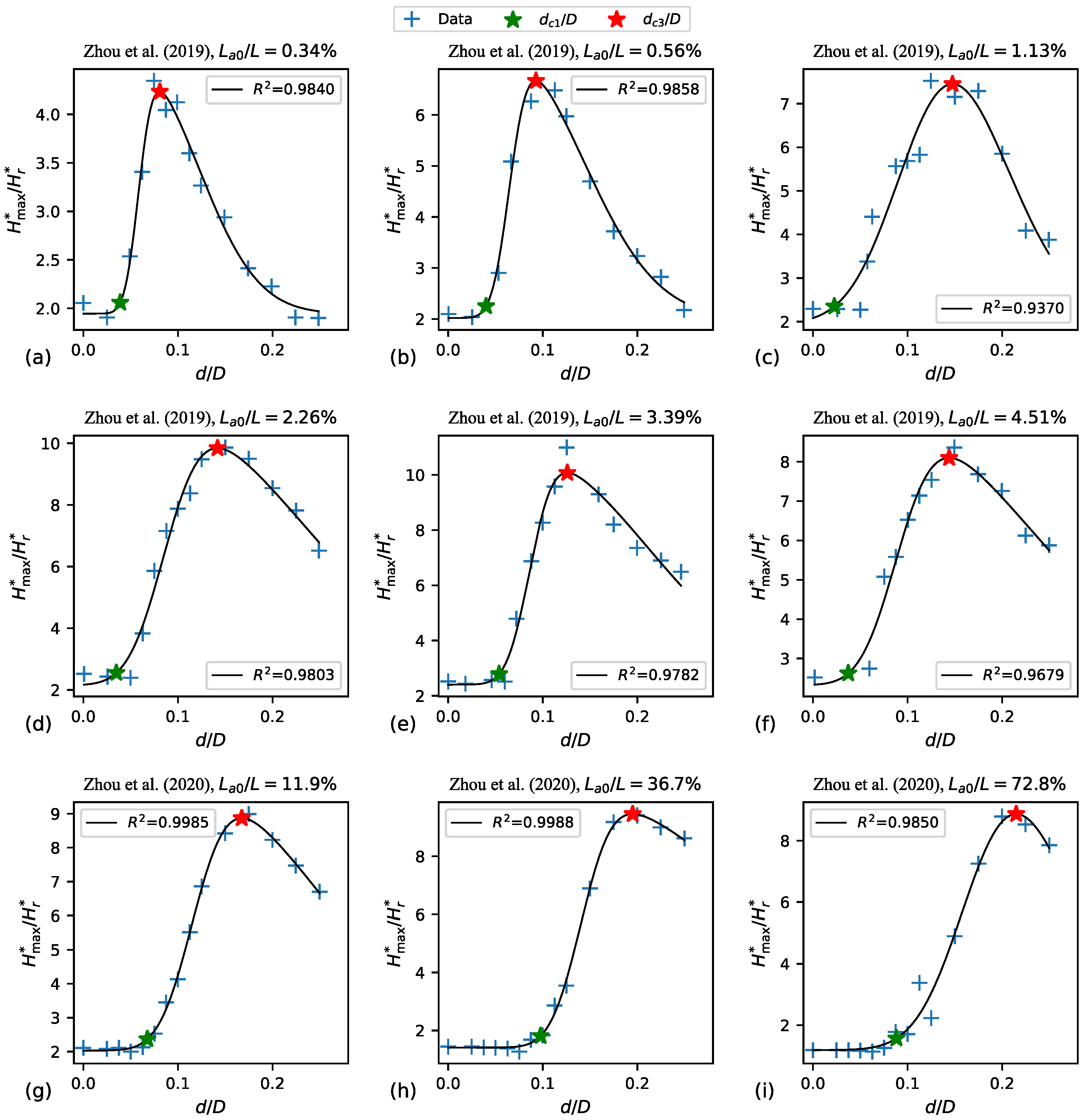
Figure 23 presents the data from Zhou et al. (2019) [
39] and Zhou et al. (2020) [
3] concerning the filling procedure with
. This figure also presents both the curves that represent the data (i.e., right-skewed probability density curves fitted to the data) and the
and
values associated with each curve. Only data within the range of
was considered for two main reasons. Firstly, very large
values are generally not considered in practice. Secondly, these larger
values sometimes correspond to transient magnitude values lower than the low left plateau of the data. This poses challenges for fitting the representational curves, as the chosen function for fitting the data assumes identical vertical axis values for both the left and right low plateaus. Not imposing this limitation on the considered
range for curve fitting would compromise the predictive accuracy of the fitted curve for type 1 behaviour.
In
Figure 23a–f (with data from Zhou et al. 2019 [
39]), the
values range from 0.023 to 0.054, while the
values range from 0.081 to 0.148. In
Figure 23g–i (with data from Zhou et al. 2020 [
3]), the
values range from 0.068 to 0.098, while the
values range from 0.167 to 0.215. The critical
values identified in the current study (which are presented in
Table 1) exhibit greater similarity to those reported in Zhou et al. (2019) [
39] than to those reported in Zhou et al. (2020) [
3]. This analysis indicates that the critical
values for both type 1 and type 3 behaviours are notably influenced by the specific characteristics of each system and the transient event. Note that the definitions used herein for type 1 and type 3 behaviours differ from those used in Zhou et al. (2019) [
39] and Zhou et al. (2020) [
3]. While not necessarily indicating a direct cause-and-effect relationship, similar to the current study, the experiments carried out by Zhou et al. (2019) [
39] involved significantly reduced air fractions. Additionally, when compared to a horizontal filling procedure as examined in Zhou et al. (2020) [
3], vertical filling procedures and the air expulsion stage with inclined pipe segments connected to the air valve are expected to exhibit a more predictable air–water interface behaviour.
7.5. Non-Slam Air Valves
To implement in practice the concept of enabling unrestricted inflow while restricting outflow, a non-slam air valve can be employed. A typical non-slam air valve contains two floats, which do not hinder air inflow. With the air valve under a reduced positive head, they do not obstruct the air flow through the large orifice of the valve. However, if this positive head exceeds the transition head, the upper float closes, permitting air flow only through a small orifice. Both floats move to the closing position when the water reaches the valve, effectively sealing it. The main design parameters of a non-slam air valve are the diameter of the inflow orifice, the diameter of the large outflow orifice, the diameter of the small outflow orifice, and the transition head. Schematics of non-slam air valves can be found in Tran (2017) [
40] and Li et al. (2022) [
18].
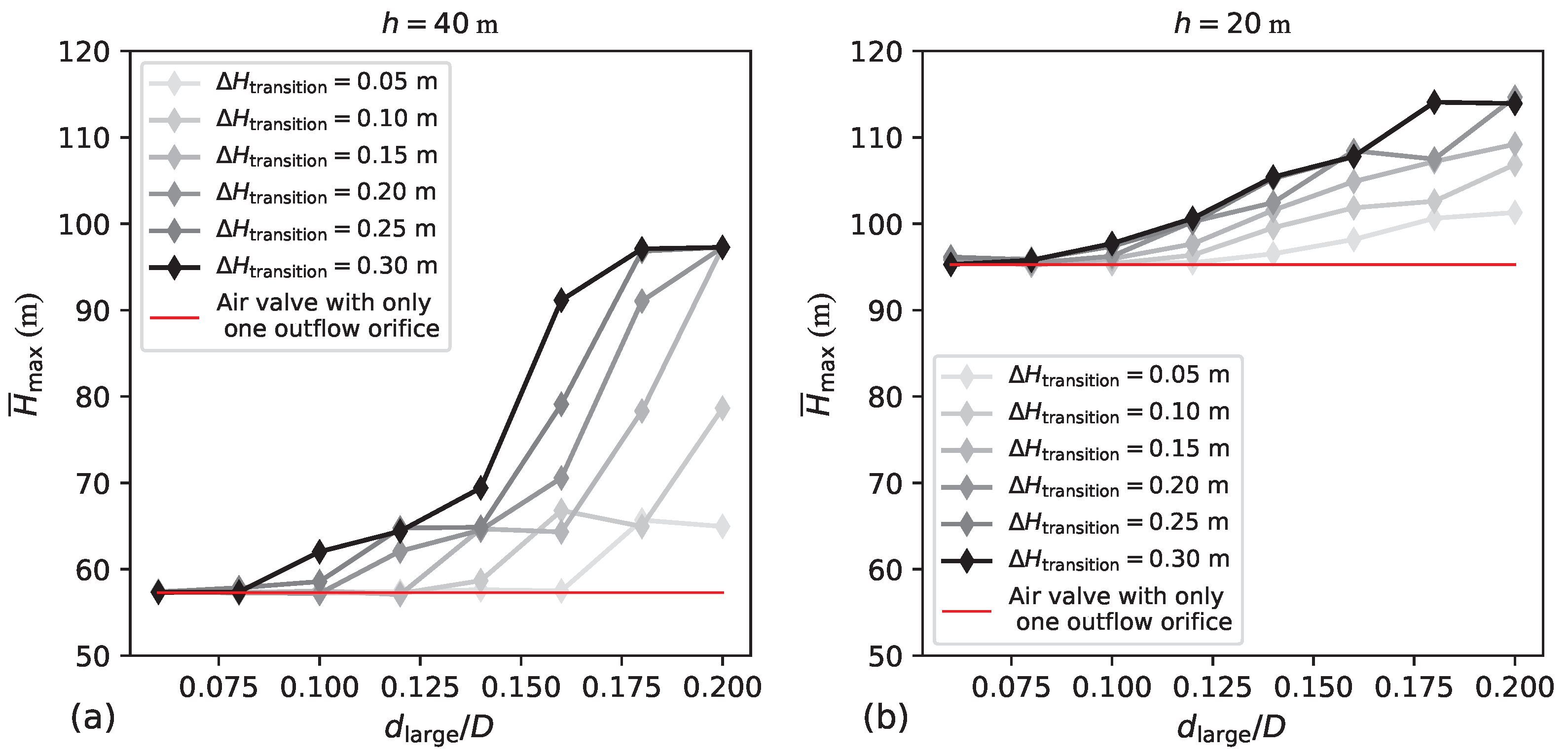
Figure 26 shows the transient response of a pipeline with a non-slam air valve during the pump trip scenario. The inflow orifice ratio is set as
. The small outflow orifice ratio is set as
, which is an orifice ratio found to be effective for transient attenuation.
Figure 26 assesses the influence of the following parameters on the transient response: transition head (
), which is the threshold head for transitioning from the large outflow orifice to the small outflow orifice; large outflow orifice ratio (
); and air valve elevation (
h). The
values considered in this figure are in line with typical values found in product catalogues.
As shown in
Figure 26, in general, as
decreases, the behaviour of the non-slam air valve becomes more similar to that of the air valves with a single and small outflow orifice. This similarity becomes most pronounced when the
value falls below a specific threshold for each
value. This
threshold decreases as
increases.
Figure 26 highlights the importance of carefully selecting both
and
. In this sense, inadequate selection of these parameters may render the non-slam air valve ineffective in mitigating transients. This can happen if
is oversized so that
is never reached, or if
is too large for a given
value.
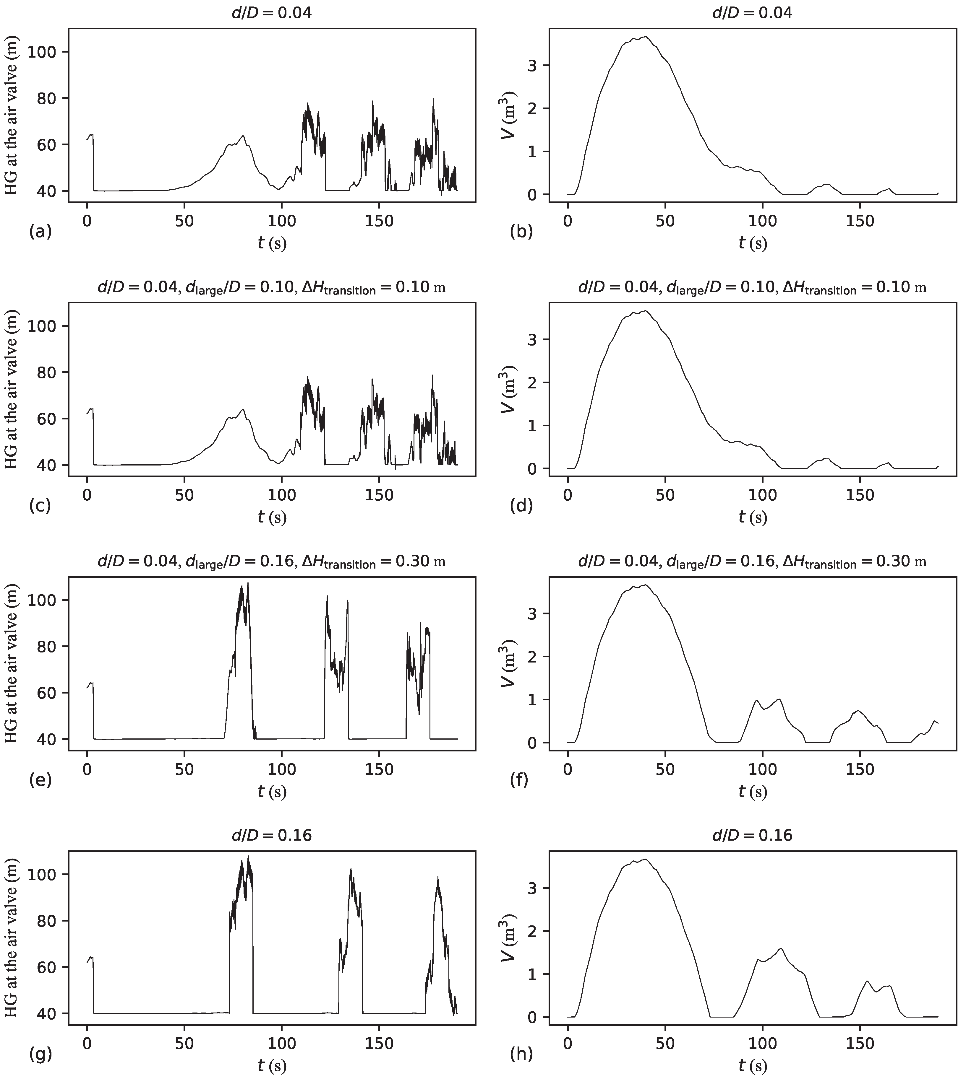
Figure 27 shows the evolution of both the HG at the air valve and the air pocket volume across four distinct situations: air valve with a single and small outflow orifice (
Figure 27a,b), effective non-slam air valve (
Figure 27c,d), ineffective non-slam air valve (
Figure 27e,f), and air valve with a single and large outflow orifice (
Figure 27g,h). For the non-slam air valve with
and
m (
Figure 27c,d), the transient response is similar to the case with the air valve with a single and small outflow orifice (
Figure 27a,b). However, for the non-slam air valve with
and
m (
Figure 27e,f), the air valve fails to attenuate the transient event. In fact, the transient response for the case with the air valve with a single and large outflow orifice (
Figure 27g,h) is similar to the case with the ineffective non-slam air valve (
Figure 27e,f). Notably, having a small
value or a small
value might render the air valve unsuitable for pipeline filling, which usually requires a high air exhaust rate.

 ,
, 


