Groundwater Flow Model along a Vertical Profile of the Sardas Landfill in Sabiñánigo, Huesca, Spain

Abstract

Lindane (a harmful contaminant) was produced in Sabiñánigo (Huesca, Spain) and deposited at the Sardas landfill. This site contains a large mass of pollutants, which have an extremely large contamination potential of the Ebre River. The site has undergone numerous human interventions that have modified the natural conditions. The site exhibits complex hydrogeological patterns and has been monitored systematically for a long period of time, and a large amount of geological, hydrological, and hydrogeological data are available. Here, a 2D finite element groundwater flow model along a vertical profile heading east–west along the thalweg of the former gully is presented. The main goal is modelling groundwater flow through the landfill, the Gállego River alluvial aquifer, and its interactions with the Sabiñánigo reservoir. The numerical model confirms the prevailing conceptual hydrogeological model of the site. The main results include: (1) Groundwater flows into the landfill mainly along perimeter ditches, which do not properly drain the surface and subsurface runoff (13.84 m³/d) and from the underlying marly rock (8.84 m³/d); (2) The total landfill leachate outflow towards the alluvial floodplain underneath the front slurry wall through a shallow marl layer is equal to 17 m³/d; (3) The oscillations of the Sabiñánigo reservoir water level produce a tidal effect that results in periodic changes of the hydraulic gradient between the alluvial gravels and the reservoir; (4) Groundwater flows generally from the alluvial aquifer towards the reservoir in an average E–W direction with an average Darcy velocity equal to 5 cm/d. The flow direction, however, changes to W–E when the reservoir level rises suddenly and; (5) The hydrodynamic parameters of the alluvial silts and reservoir silting sediments are crucial in determining the influence radius of the inversion of groundwater flow direction when the reservoir level rises suddenly. Model results enhance the confidence of the conceptual model, provide the basis for detailed specific models of the landfill and the alluvial aquifer, and highlight the importance of considering the tidal effect of the reservoir level oscillations. They also provide valuable information for managing the landfill and its impact on the surrounding groundwater system.

1. Introduction

Technical hexachlorocyclohexane (HCH) is an organochlorine pesticide mixture of five main isomers α-HCH, β-HCH, γ-HCH, δ-HCH, and ε-HCH. It was used in agriculture in the 1950s and 1960s due to its effectiveness and low cost [1]. However, the discovery of its harmful effects on human health and plant growth [2] led to the isolation of the δ-HCH isomer, which is the only isomer with insecticide properties. Lindane (which contains >99% of the δ-HCH isomer) was thought to be tasteless, harmless, and safer [3]. Vijgen [4] reported that 6 to 10 tons of HCH waste isomers were generated for each ton of lindane produced, which were primarily disposed near the production sites [5]. These residues were initially considered innocuous due to their relatively low solubility in water [6]. The low solubility of Chlorinated Organic Compounds (COCs), constituting this organic phase, poses a significant risk to both groundwater and nearby surface waters [7].

The European Union banned lindane in 2008, and the HCH isomers were included in the Stockholm Convention’s list of Persistent Organic Pollutants in 2009 due to their persistence, toxicity, and potential to bioaccumulate in the food chain [8,9,10]. Organochlorine pesticides also pose a threat to biodiversity and pollination and could endanger many species [11,12]. A total of 29 landfill sites were identified as primarily dedicated to receiving HCH wastes and connected to large production facilities [13]. The LINDANET project identified fifteen regional actions as good practices, acknowledging the complex and site-specific challenges posed by each polluted site [14].

The persistent nature of HCH waste contribute to its retention in landfills for prolonged periods, possibly spanning decades to centuries [6]. The release of Persistent Organic Pollutants (POPs) from landfills is partly influenced by water solubility and volatility, as well as the characteristics of their respective landfill environments [6]. HCH isomers’ great stability and longevity in water [11] contribute to its frequent detection in groundwater [15].

Spain has several sites affected by lindane production including the INQUINOSA factory in Sabiñánigo, Huesca. INQUINOSA disposed powder and liquid residues from lindane production at the Sardas and Bailín landfills [16]. The Sardas landfill contains lindane production wastes, including a dense non-aqueous phase liquid (DNAPL) containing HCH isomers, benzene, and chlorobenzenes [17]. These liquid residues were generated during lindane production from failed chlorination reactions and distillation [7].

To mitigate potential environmental impacts, the Sardas landfill perimeter was sealed in 1995 with a concrete wall that reached the underlying marls to prevent water inflows from the surrounding rock. Perimeter drainage ditches were constructed to collect surface and subsurface runoff from the landfill, but they do not collect all the surface runoff and subsurface flow, resulting in water flowing underneath the concrete wall into the Sardas landfill. The hydrogeological classification system for municipal solid waste landfills, as presented in Zhan [18], categorizes the Sardas landfill as a landfill with valley landform classification, characterized by intensive runoff.

The landfill is located less than 500 m east of the Sabiñánigo reservoir, which was created in 1963 on the Gállego River course to provide hydroelectric power to neighboring towns and factories. Water inflows into the landfill include the water that seeps into the landfill underneath the perimetral concrete wall and also some groundwater flow from the surrounding marly bedrock (solid rock underlying the landfill) [16,19]. EMGRISA [20] identified a preferential flow path in an east–west direction following the natural terrain gullies and a hydraulic connection between the landfill and the river alluvial sediments. The front slurry wall was supposed to seal the landfill. However, landfill leachates flow through the underlying marls into the Gállego River alluvial aquifer composed of sands and gravels. The gravel layers are the most permeable materials. Groundwater finally discharges into the Sabiñánigo reservoir through the alluvial silts and the silting sediments. Santos [17] reported that DNAPL pollution could have already affected the Gállego River alluvial aquifer.

The Sardas site was selected for numerical modeling because it presents several unique features. First, this site contains a large mass of pollutants. The Sardas landfill is estimated to contain between 30,000 and 80,000 tons of solid HCH [16]. This compound has an extremely large contamination potential because 1 g of HCH can pollute up to 10 hm³ of Gállego River water. Finally, the Sardas site has been monitored systematically for a long period of time, and therefore a large amount of geological, hydrological, and hydrogeological data are available.

The Sardas site has undergone numerous human interventions that have modified the natural hydrological and hydrogeological conditions of the site. In addition, the large heterogeneity of landfill wastes poses an important challenge. A 2D finite element groundwater flow model along a vertical profile of the Sardas landfill site is presented here to quantify the interactions of the Sardas landfill, the Gállego River alluvial, and the Sabiñánigo reservoir.

The modelling methodology starts with the formulation of the conceptual model based on the available hydrogeological and hydrodynamic data of the site (Figure 1). The conceptual model includes the main hypotheses and the definition of the initial and boundary conditions and parameter zones. The finite element method is used to discretize the partial differential equation of flow into algebraic equation. Model calibration is needed to improve the estimation of the hydrogeological parameters and is performed by comparing calculated values with measured values of key hydrogeological variables such as groundwater velocity and hydraulic head, which measures the energy of a groundwater sample per unit weight of water.

Model results have significantly contributed to the improvement in understanding the Sardas landfill and its surroundings, as well as the robustness of the conceptual model of the site.

Models and the data used to construct them have uncertainties, and these uncertainties affect the assessment of groundwater sustainability. Samani et al. [21] present seven indicators to evaluate the sustainability of aquifers. These indicators were integrated in a time series method to calculate the overall sustainability. The method provided insight into the overall stability of aquifers. Samani et al. [22] present statistical and machine learning methods for groundwater level response identification by using meteorological data.

2. Materials and Methods

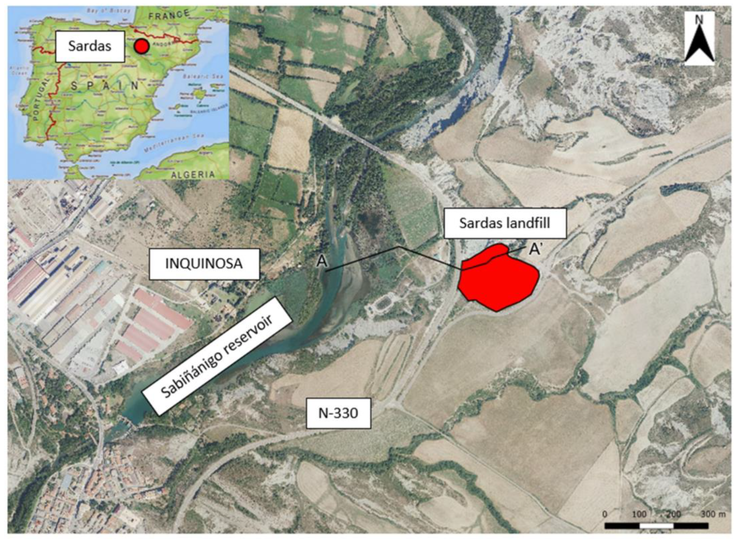
2.1. Site Description

In 1963, the Sabiñánigo reservoir was built in the Gállego River course in Sabiñánigo, Huesca in the northeast of Spain. The reservoir occupies a large part of the alluvial floodplain and lower terraces. Originally spanning 26.6 hm² the reservoir volume was equal to 1.16 hm³ and maximum depth was equal to 14 m near the dam. However, the accumulation of reservoir silting sediments since its construction in 1963 has reduced its maximum depth to less than 5 m and its volume to 0.093 hm³ in 2009 [23].

INQUINOSA operated from 1975 to 1988 and deposited HCH wastes in the Sardas landfill located less than 500 m to the west of the Sabiñánigo reservoir (Figure 2) and occupying an area of nearly 40,000 m². In the 1980s, the Sardas landfill was filled with more than 400,000 m³ of urban, construction, and industrial solid wastes (Figure 3), and INQUINOSA began depositing wastes in the Bailín landfill located more than 3 km to the south. It is estimated that between 30 and 80 × 10⁶ kg of the wastes deposited in the Sardas landfill are residues from lindane production, in powder and liquid states [16].

In the 1990s, during the construction of the N-330 road about 50,000 m³ of landfill wastes were relocated on top of the floodplain of the Gállego River [20] (Figure 3). In 1995, the Sardas landfill was sealed superficially and laterally. In the downstream section of the landfill, a 75 m-long and 0.5 m-thick slurry wall with variable depth up to the underlying marls was built to serve as a barrier to the groundwater discharge from the landfill (Figure 3). On the other hand, the landfill perimeter was sealed using a 0.5 m-thick concrete wall that reached the underlying marls to prevent water inflows from the surrounding marly rock. Perimeter drainage ditches were installed atop the concrete wall to collect the landfill’s surface runoff and interflow.

In 2009, a DNAPL composed of HCH isomers, benzene, and chlorobenzenes was found in the landfill waste [17]. This prompted immediate collection efforts and hydrogeological studies focused on identifying containment and treatment options for future implementation [16] (Figure 3).

There are several point sources of pollution (hot spots) in the site: (1) INQUINOSA former production site, (2) the Sardas landfill, (3) the landfill wastes spread out in the alluvial, and (4) two leachate ponds. INQUINOSA operated from 1975 to 1988. The conducted assessments have revealed significant soil and groundwater pollution in its former production site [16].

The Sardas landfill rests on top of gray Larrés Marls, which exhibit steep slopes and abundant scree at their base, are highly erodible, and form a characteristic landscape of gullies and badlands. Downstream the landfill, the Larrés marls underlie the quaternary sediments of the Gállego River alluvial, which include a silt layer and a sand and gravel layer [24] (Figure 3). The upper layer is composed of sandy silts with higher clay content in shallower areas, and intercalations of sandy sections in other areas. This layer ranges from 5 to 10 m in thickness. The underlying horizon is composed of sands and gravels with highly variable grain sizes and a clay matrix, about 5 m thick. The Sabiñánigo reservoir substrate consists of gray marls and cemented sandstones, as well as quaternary deposits that range from 1 to 12.5 m thickness overlaid by clays, silts, and fine sands. Silting sediments of the reservoir show gray shades, and it is possible to distinguish black bands with a large content of oxidized organic matter [25].

Larrés Marls present varying hydraulic conductivities due to the presence of fractured, altered, and decompressed zones [19]. The shallow layer, known as FAD, is more fractured and altered than the deeper marls, resulting in a higher hydraulic conductivity. FAD thickness ranges from 0.5 m to 5 m [19].

The quaternary deposits in the upper layer of the Gállego River alluvial have a hydraulic conductivity much smaller than that of the underlying horizon composed of sands and gravels.

Available data show that landfill leachates flow underneath the front slurry wall through the shallow marls. On the other hand, the landfill perimeter drainage ditches installed atop the concrete wall to collect the landfill’s surface runoff and interflow allow part of the runoff to flow into the landfill underneath the concrete wall. Groundwater flow through the Gállego alluvial takes place mostly through the sand and gravel layers.

2.2. Conceptual Model

The numerical groundwater flow models focus on the hydrogeological characteristics of the main geological bodies, which include (listed from west to east): (1) A shallow layer of alluvial silt overlying a layer of sands and gravels, which in turn rest on a thick layer of marls [24]. This layer extends from the west and is limited by the front slurry wall; (2) the landfill wastes spread out in the alluvial at the foot of the landfill [16]; (3) the landfill fillings upstream of the front slurry wall, which include the anthropogenic wastes overlying the marls and a patch of marl erosion silts in the intermediate area between the landfill wastes and the marls; and (4) the geological materials upstream the landfill, which include a narrow glacis layer overlaying the shallow layer of marls (Figure 3 and

Table 1. Thickness, depth, and prior information on hydraulic conductivities of the geological layers.

Geological Layer	Thickness (m)	Depth (m)	Prior Information of Hydraulic Conductivity (m/d)
Alluvial silts	5–10	0–10	0.01–0.1
Alluvial sands and gravels	5	10–15	10–100
Landfill wastes spread throughout the alluvial plain	0–5	0–5	-
Landfill wastes	0–40	0–40	3–21
Surrounding marly rock	2–6.5	0–6.5	<0.0001
Fractured marls	0.5–5	-	0.04–0.18
Deep unfractured marls	Up to 100 m	5–30	<0.0001

). The average thickness of the FAD layer is estimated equal to 5 m, which is within the range of values reported by [19].

Upstream the front slurry wall, groundwater flows from the natural marly rock into the landfill underneath the perimeter concrete wall (Figure 3). The landfill wastes are connected to the alluvial through the superficial layer of the marls (FAD). Then, groundwater flows vertically through the spread out wastes and alluvial silts into the sand and gravel layer, which is the most permeable layer in the site. Sands and gravels are connected to the reservoir through the silts and the silting sediments of the reservoir (Figure 3).

A profile heading east west along the main gully has been selected for the two-dimensional flow models, which follows the trace of boreholes SE23, PS26B, PS21, PS14, PS14L, PS19B, PS19C, S37, S37B, S39B, S39F, and S35E as shown in Figure 4. Additionally, boreholes PS26, PS21B, PS5D, PS5E, PSF, PS5G, PS29B, PS29C, S44D, and S39 that are near the profile trace and provide relevant information to calibrate the model have been considered.

The conceptual flow model of the site is based on the following assumptions: (1) The flow is contained in the vertical plane defined by the profile trace with a unit thickness; (2) an average apparent width of the landfill of 50 m has been assumed to convert the inflows and outflows of the landfill into flows per unit length; and (3) the fractured, altered, and decompressed marls are treated as an equivalent porous medium.

2.3. Numerical Model

2.3.1. Finite Elements Mesh and Parameter Zonation

The numerical 2D horizontal model domain was discretized by using a triangular finite element mesh, consisting of 3020 nodes and 5717 elements (Figure 5). The mesh was refined around the Gállego River alluvial and the front slurry wall. The profile has a total length of 618 m, with the upper boundary of the domain coinciding with the average water table and potentiometric surface estimated from a preliminary steady state model. The lower boundary was set at an elevation of 710 m, while the maximum elevation of the upper boundary was 816.43 m.

The simulations were performed in steady-state and transient regimes. A transient flow model with time increments of 1 day was performed from 1 January 2013 to 29 September 2022. A transient flow model with time increments of 30 min was performed from 3 July to 5 November 2018. The daily multiannual transient flow model aims at studying the seasonal evolution of the groundwater flow, while the transient state model with time increments of 30 min aims at analyzing the fluctuation of the piezometric level in the alluvial of the Gállego River caused by the oscillations of the Sabiñánigo reservoir water level.

Hydraulic heads and reservoir levels were recorded by EMGRISA [26,27] with automatic and manual hydraulic head measurements devices. EMGRISA also performed the sampling campaigns by following standard sampling protocols.

The spatial variability of hydrogeological parameters was accounted for in the model by defining 17 material zones, with all elements within each zone sharing the same hydrodynamic parameters (

Table 2. Calibrated hydrogeologic parameters in the material zones of the vertical profile numerical model. FAD marls = fractured, altered, and decompressed marls. Colors are used to identify the material zones shown in Figure 5.

Material Zone	Color	Hydraulic Conductivity K (m/d)	Storativity SS (m−1)
Silting sediments		0.10	2·10−4
Alluvial silts A		0.01	10−4
Alluvial silts B		0.01	10−4
Alluvial silts C		0.01	10−4
Gravels		300	2·10−4
Landfill wastes spread throughout the alluvial plain A		0.30	7·10−4
Landfill wastes spread throughout the alluvial plain B		1.00	7·10−4
Landfill wastes A		15	8.5·10−4
Landfill wastes B		5.00	8.5·10−4
Landfill wastes C		0.08	10−4
Marl erosion silts		0.15	2·10−4
Glacis		0.25	0.20
FAD marls A		0.03	5·10−5
FAD marls B		0.035	5·10−5
FAD marls C		5.5·10−3	5·10−5
Deep marls		10−6	10−5
Front slurry wall		10−6	10−5

). Prior estimates of hydrogeological parameters were derived from field hydraulic tests including slug and long-term pumping tests [20]. The final parameter values were obtained from model calibration by improving the fit of the computed hydraulic head oscillations to the measured hydrographs in monitoring boreholes.

2.3.2. Boundary Conditions

Figure 5 depicts the mesh scheme and boundary conditions used in the groundwater flow model. Inflows include the infiltration recharge, groundwater recharge from the surrounding marly rock and inflow through the landfill perimeter drainage ditches. A hydrological water balance model was developed by using the VISUALBALAN code [28] which computes the daily water balance in the soil, in the unsaturated zone, and the aquifer. Water balance models were performed in the alluvial floodplain, the landfill cover, and the natural marly rocks. These models account for net interception and net evapotranspiration and provide estimates of groundwater rates. The total precipitation recorded in the meteorological station installed at the site accounts for rainfall, snow, and water vapor condensation. The conditions of the site do not favor a lot of water vapor condensation, and therefore we claim that water vapor condensation is not relevant in our study area. In our model, water vapor condensation is lumped into the net daily evapotranspiration, ET. We think that this condensation does not have a significant impact in the model results because groundwater recharge is estimated with acceptable accuracy from available hydraulic head data.

Even though the precipitation is the same in the alluvial floodplain, the landfill cover, and the natural marly rocks, there are large differences in recharge rates because the landfill cover prevents the recharge into the landfill, and the natural terrain has strong slopes that favor surface runoff. The results of the hydrological models indicate that the mean annual recharge values in the alluvial floodplain, landfill surface cover, and surrounding marly rock are equal to 149 mm/year, 14 mm/year, and 37 mm/year, respectively.

The numerical groundwater flow model also accounts for groundwater recharge from the surrounding natural marly rock that flows into the landfill through the gully near borehole S35E, with an average inflow of 8.84 m³/d. Measured hydraulic heads and pumping tests show that the perimeter recharge is most relevant in the lowest parts of the landfill near the northwest corner, with an average recharge of 7.47 m³/d in this area and 4.37 m³/d through the rest of the perimeter ditches. The hydrological balance model provided the time evolution of infiltration recharge (Figure 6), inflow from the surrounding marly rock (Figure 7), and recharge from perimeter ditches (Figure 8) considered in the groundwater flow model. Annual average precipitation in the recharge plain is significantly higher than recharge in the landfill cover layer, and in the natural marly rock.

At the foot of the landfill, a discharge zone near borehole PS29C is simulated to account for the reported seepage area. The Sabiñánigo reservoir flood plain boundary is simulated with a Dirichlet-type boundary condition, with an external head equal to the reservoir water level recorded by the Automatic Hydrological Information System (SAIH) every 15 min. The reservoir water level ranges from 764.04 m to 765.57 m between 21 November 2014, and 4 February 2022. To account for water levels measured from 1 January 2013 to 20 November 2014, measurements on the same day from the earliest available year have been used. The daily multiannual transient state is calculated by considering the average daily reservoir water level, whereas the 4-month simulation uses the reservoir water level monitored every 30 min (Figure 9).

The model accounts for the water pumping in borehole S37 (Figure 10), located upstream the front slurry wall. Pumping started in June 2014 and continued intermittently until March 2022 when it was halted. The average pumped rate in this period is equal to 5.97 m³/d. In the 2D model of the vertical profile, the pumping flow is distributed over an “apparent width” of the landfill equal to 50 m and is distributed uniformly along the saturated thickness of the S37 borehole. To approximate the radial flow produced by three-dimensional pumping, three reinjection nodes with a Cauchy condition were considered. The external head of the reinjection nodes was assumed constant and equal to the measured hydraulic head in nearby boreholes. The leakage factors for this Cauchy condition were calibrated.

2.3.3. Computer Code

The flow model was performed with CORE^2D V5, a finite element code for transient saturated and unsaturated water flow, heat transport, and multicomponent reactive solute transport in heterogeneous and anisotropic media [29]. CORE^2D V5 has been extensively verified against analytical solutions and other reactive transport codes [30] and widely used to model groundwater flow and solute transport in real-world aquifers [31], laboratory and in situ experiments (pp. 90–91), and the long-term geochemical evolution of radioactive waste repositories.

3. Results

Calibration data include measured hydraulic heads, seepage discharge near the PS29C borehole, and Darcy velocity measured at PS16H borehole. Calibration was performed by ensuring that the computed hydraulic heads h are smaller than ground elevation, z. Model performance was evaluated by the statistical analysis of the hydraulic head residuals, which are defined as the differences between the computed and the measured heads.

3.1. Steady-State Flow Model

The model calibration involved successive runs in steady-state regime focused on minimizing hydraulic head residuals. The seepage discharge rate near the PS29C borehole recorded by EMGRISA was also calibrated. Considering surface water discharge observations to the calibration greatly reduces predictive uncertainties [32].

Figure 11 depicts the contour plots of the hydraulic head computed in a steady-state regime.

3.2. Transient-State Flow Model with Daily Time Increments

The computed hydrographs between 1 January 2013, and 29 September 2022, in the river alluvial boreholes are closely related with the reservoir water level indicating the high hydraulic conductivity of the sand and gravel layer. However, they also show a slight lag and damping. Overall, the model accurately reproduces the magnitude of the hydraulic head fluctuations in these boreholes (Figure 12).

The model also reproduces the hydraulic head measured throughout the embankment of the N-330 road, from upstream the front slurry wall (S37 borehole), downstream the front slurry wall (S37B borehole) as shown in Figure 13, on the other side of the N-330 road (S44D borehole), and at the end of the N-330 road embankment and beginning of the alluvial floodplain (PS29B and PS29C boreholes) as shown in Figure 12.

The groundwater balance during the simulation period shows that most of the groundwater recharge into the landfill flows through the perimeter ditches of the landfill with an average inflow of 13.84 m³/d (41%) and from the surrounding marly rock at the head of the landfill with an average inflow of 8.84 m³/d (31%). Groundwater in the alluvial systems flows horizontally through the sands and gravels and discharges mostly to the Sabiñánigo reservoir flowing vertically upwards through the alluvial silts and silting sediments. Sabiñánigo reservoir outflow is equal to 16.26 m³/d (54%). The seepage area located at the foot of the landfill discharge is equal to 9.05 m³/d (30%) and the average pumping rate in the simulation period is equal to 4.79 m³/d (16%). Recent results reported in [33] indicate that water recharge along the landfill perimeter is notably largest at the lowest northwestern corner of the landfill.

3.3. Transient-State Flow Model with 30’ Time Increments

The computed hydrographs in boreholes PS26, PS26B, PS21, PS21B, PS14, and PS19B, which are screened in sands and gravels, confirm that the head fluctuations in this layer are strongly affected by the oscillations of the Sabiñánigo reservoir water level (Figure 14).

Groundwater flow velocity in gravels is much higher compared to other layers. At the same distance from the reservoir, the Darcy velocity in FADs is two orders of magnitude lower than in gravels. The flow is generally towards the reservoir, except when the Sabiñánigo reservoir water level increases suddenly, causing a reversal of the flow direction (Figure 15 and Figure 16). This effect is observed in the PS26 borehole, but not in the PS16 borehole.

4. Discussion

4.1. Steady Flow Regime

The average residual is equal to 0.023 m while the mean absolute residual is equal to 0.35 m. Other statistics include: median = 0.02 m, standard deviation = 0.5756 m, skewness = −0.60, and kurtosis = 3.33 (see Table S1 in the Supplementary Materials, SM). All absolute values of the residuals are smaller than 2 m. The root mean square error normalized by the standard deviation (NRMSE) is equal to 0.05 and the Nash–Sutcliffe index [34] is equal to 0.9972. Figure 17 shows the sample histogram and quantile-quantile (q-q) plot of model residuals. All these statistics attest that the model fit is excellent and thus enhances the confidence on the proposed conceptual model, the boundary conditions, and the hydrogeological parameters.

The initial hydraulic conductivities in the model were derived from pumping and slug test performed in boreholes drilled in different layers [20]. Subsequently, following model calibration, the hydraulic conductivity values were refined.

Table 3. Prior information and calibrated hydraulic conductivities.

Geological Layer	Prior Information of Hydraulic Conductivity (m/d)	Calibrated Hydraulic Conductivity (m/d)
Alluvial silts	0.01–0.1	0.01
Sands and gravels	10–100	300
Landfill wastes located near the front slurry-wall	3–21	5–15
Fractured shallow marls	0.04–0.18	5.5·10−3–0.03

shows the comparison between the initial hydraulic conductivities and the calibrated values.

The highest residuals are calculated in the S39 series boreholes, located along the old north gully where most of the waste from the INQUINOSA factory was deposited. Boreholes of the S39 series show similar measured hydraulic heads but show some discrepancies. The borehole S39M hydraulic head (792.13 m) is higher than the hydraulic head measured in borehole S39G (791.73 m), despite S39M being located downstream S39G. Similar discrepancies are observed in boreholes S39L (792.10 m) and S39F (791.89 m). While S39F is located upstream S39L, it has a higher average measured hydraulic head. According to EMGRISA, the presence of DNAPL in the boreholes may affect the head measurements. In addition, small-scale heterogeneities have the potential to create perched aquifers, offering a plausible explanation for the inconsistencies encountered in the measured head.

Groundwater models of aquifers influenced by both intricate natural dynamics and human activities can entail inherent uncertainties [35]. Model errors and uncertainties encompass errors in the data, uncertainties due to insufficient geological and hydrogeological data, and errors linked to the conceptual model structure, with the assumption of 2D vertical flow being a notable source of potential error in this study. Numerical model uncertainty could also affect the results [36].

The contour plots computed hydraulic heads show that the hydraulic gradient in the sands and gravels of the alluvial is very small because their hydraulic conductivity is very large (Figure 11). The reservoir water level oscillations significantly affect the heads in the alluvial boreholes. The hydraulic gradient is also small in the lower part of the landfill, upstream of the front slurry wall. Pumping test and hydraulic head measurements showed that the permeability of the landfill wastes is higher in the lower part of the landfill. There is a substantial water table drop in the wastes spread out in the alluvial (from the S37B borehole to PS29 boreholes) and a high vertical hydraulic gradient at the foot of the landfill, around the PS19B (screened in the sand and gravel layer) and PS19C (screened in the silt layer) boreholes.

4.2. Transient Flow Regime with Daily Time Increments

The slight lag and damping between the reservoir water level and the alluvial boreholes hydraulic heads indicates that silting sediments and, in some areas, silting sediments and underlying alluvial silts are interposed between the reservoir water and the sands and gravels of the alluvial. The fluctuating groundwater exchange between the sands and gravels of the Gállego alluvial and the Sabiñánigo reservoir has been analyzed in [37] with a detailed numerical model, which accounts for 2D horizontal groundwater flow through the Gállego alluvial.

The model accurately reproduces the vertical hydraulic gradient existing between the PS19C borehole that is screened in the alluvial silts and the PS19B borehole that is screened in the alluvial sands and gravels (Figure 12). However, the hydraulic head measured in the PS19C borehole shows greater oscillations than the hydraulic head measured in PS19B borehole. The model does not reproduce this greater variability recorded in borehole PS19C. The hydraulic head measured with a diver in borehole PS19C shows sudden oscillations, which could be caused by surface water inflows into the borehole. These sudden head rises take a long time to dissipate due to the low vertical hydraulic conductivity of the alluvial silts (see Figure S1 in Supplementary Materials).

The hydraulic heads measured in PS5D and PS5G boreholes, which are screened in the alluvial sands and gravels, are lower than those recorded in the PS5E and PS5F boreholes, which are screened in the alluvial silts. Model results reproduce the vertical gradient of hydraulic heads between the silts and gravels of the Gállego alluvial (Figure 12). The computed hydraulic head in the PS5D and PS5G boreholes are strongly affected by the reservoir level, with a lag and damping. However, the lack of continuous hydraulic head measurements prevents evaluation of the good fit of the measured hydraulic head in these two boreholes. The numerical model is unable to match the time evolution of the measured heads in the PS5E and PS5F boreholes, which vary more than the computed hydraulic heads. Part of the sudden hydraulic head fluctuations in these two boreholes could be caused by surface water infiltration, which then can take months to decrease due to the low vertical hydraulic conductivity. The PS5F borehole shows an almost constant hydraulic head between March and December 2021, and it is suspected that the water table may be below the level of the borehole bottom (see Figure S2 in Supplementary Materials).

The hydraulic head in the PS29B borehole is slightly higher than the measured hydraulic head, while in the PS29C borehole, the computed hydraulic head is slightly lower than the measured hydraulic head (Figure 12). The average measured hydraulic head in the S37B borehole located 2–3 m downstream of the front slurry wall is 779.14 m, while the average measured hydraulic head in the S44D borehole located 16–17 m downstream of the front slurry wall is 778.39 m, and the average measured hydraulic head in the PS29C borehole located 36–37 m downstream of the bentonite front screen is 774.02 m. This shows the existence of two material zones in the embankment of the N-330 road: one more permeable between the front slurry wall and the S44D borehole and another less permeable between S44D and PS29C.

The time evolution of the computed hydraulic head in boreholes of the S39 series shows two distinct parts (Figure 13). The first part ranges from January 2013 to November 2015, while the second part ranges from November 2015 to September 2022. The model reproduces the hydraulic head measured between 2013 and 2014 in the S39B borehole. However, the computed hydraulic head is lower than the measured head after January 2016. In the S39F and S39 boreholes, the model matches the computed hydraulic head better between November 2015 and September 2022 than before 2015.

Lastly, according to the model results, the computed hydraulic head in the S35E borehole that is screened in marls shows a decreasing trend from 2014 to 2018, which does not match the measured head (Figure 13). The fluctuations in the measured heads in boreholes of the S35 series may be associated with precipitation, so part of the oscillations could be affected by infiltration of surface water in the borehole, which could increase during winter due to the presence of snow. It is important to note that the hydrological balance model employed in this study does not incorporate the influence of snow during winter for the calculation of infiltration recharge. Moreover, in recent years a drain was constructed near the S35E borehole, which may have reduced the measured levels. Therefore, there are significant uncertainties that will require further investigation to improve the accuracy of the model in this area. Sobral et al. [33] present a fully 3D groundwater flow model of the landfill and the surrounding rocks that takes into account the impact of drainage system. Achieving an optimal fit of the measured heads in boreholes located at the head of the landfill remains a challenge.

Time evolution of the contour plots maps shows that the piezometric level in the alluvial varies every day with the reservoir water level oscillations. This effect is observed from the sands and gravels located underneath the reservoir until the end of the gravel layer at the foot of the landfill. The computed hydraulic head in the upper part of the landfill is near the surface both in July 2013 and January 2014. This area has low permeability, but there is a high inflow of groundwater from basins upstream the landfill. A decline in the hydraulic head across the entire vertical profile was observed in September 2015, which persisted until March 2020. Lower hydraulic heads could be linked to the pumping rate in borehole S37, which began in June 2014 and yielded a significant flow in March and April 2015.

4.3. Transient Flow Regime with 30’ Time Increments

Computed hydrographs match the level fluctuations in boreholes equipped with diver. However, the model does not accurately reproduce the head fluctuations monitored in the PS19C borehole which is screened in alluvial silts. Measured hydraulic head in this borehole reveals sudden fluctuations lasting about a day. While the computed head PS19C borehole is like that in the gravels, it has a higher average level and damped fluctuations. As previously noted, the hydraulic head sudden rises in the PS19C borehole could be related to the infiltration of surface water into the borehole which slowly decrease due to the low vertical hydraulic conductivity of the alluvial silts.

There are no estimations on the hydrodynamic parameters of the silting sediments. Groundwater flows through the sands and gravels in an average E-W direction. When the reservoir water level rises, the velocity of groundwater in the aquifer near the reservoir decreases slowly and even changes its direction to W-E. The tidal dynamics of the Sabiñánigo reservoir is similar to the tidal effect of other water bodies such as lakes and seas. It is well known that the tidal effect of a water body in an aquifer decreases with distance from the boundary aquifer/water body. The radius of influence of the reservoir tides depends on a large number of factors including the reservoir water level rise, the duration of the high waters, the thickness and the hydraulic conductivity of the alluvial silts and silting sediments that confine the sand and gravel layer from the reservoir [37]. The larger the hydraulic conductivities of the alluvial silts and silting sediments, the stronger the interactions between the reservoir and the alluvial sediments which results in a larger radius of influence of flow reversal. Long episodes of high reservoir water levels will result in larger areas of the alluvial aquifer affected by the reversal of groundwater [37].

The largest Darcy velocities have been computed in the gravels. Large Darcy velocities are also observed underneath the front slurry wall, in the FAD marl layer where there is a high piezometric gradient. Most landfill leachate flows to the Gállego River alluvial through the shallow marls located underneath the front slurry wall. Groundwater velocity is moderate in the landfill wastes and in the wastes spread out on the N-330 road embankment. Computed Darcy velocity is low in the alluvial silt layer and almost zero in the deep marls due to their very low hydraulic conductivity.

Results from a recent tracer test conducted in the vicinity of the PS16H borehole indicate that the average Darcy velocity in the sand and gravel layer is around 0.05 m/d. The model yields a similar average Darcy velocity equal to 0.054 m/d near the PS16H borehole.

5. Conclusions

A numerical flow model has been presented to quantify groundwater inflows into the landfill and groundwater outflows into the downstream alluvial floodplain of the Gállego River. The model corresponds to a vertical profile running east–west along the thalweg of the former gully. The main conclusions of the numerical model include:

• The results of the steady-state flow model confirm the validity of the conceptual flow model postulated by previous studies for this site.
• The water inflow to the landfill is about 21 m³/d. Most of the inflow occurs from the ravine located at the head of the landfill and through the perimeter ditches.
• The discharge from the landfill is equal to 17 m³/d and takes place mostly through the shallow marl layer underlying the front slurry wall and through the S37 pumping well (4 m³/d).
• The model reproduces the hydraulic head gradient across the slurry wall.
• Model results confirm that the underlying Larrés marls have a very small hydraulic conductivity, except for the shallow layer of the marls that are more fractured, altered, and decompressed.
• Model results also confirm that the computed hydraulic heads and water velocity vectors are very sensitive to the changes in the hydraulic conductivity of the shallow marls (FADs).
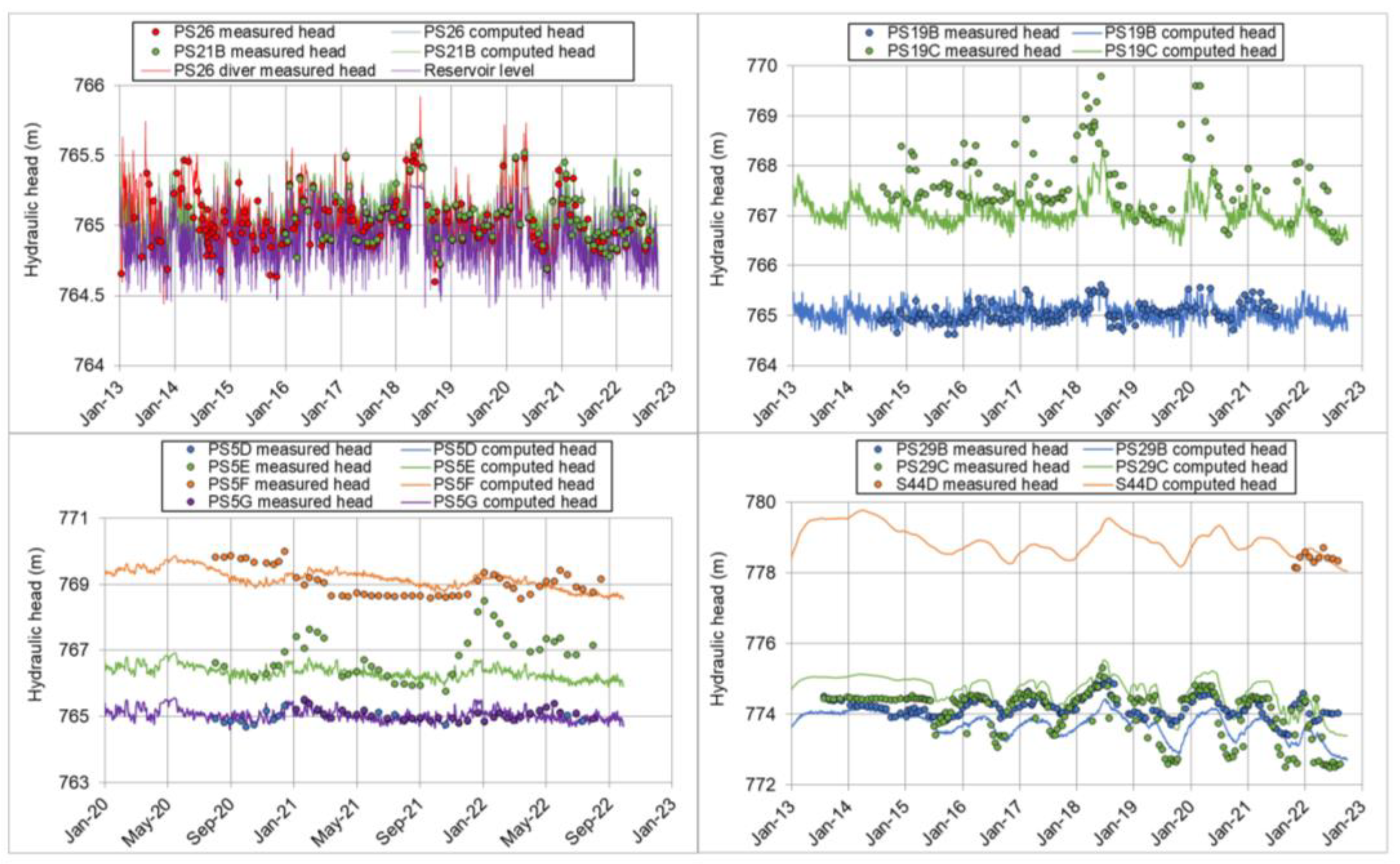
• The computed hydrographs in the alluvial boreholes match the daily fluctuations of the measured heads in the alluvial layer.
• The hydraulic heads in the alluvial boreholes show fluctuations that are strongly linked to the fluctuations of the Sabiñánigo reservoir water level. The fluctuations in the aquifer are faded and delayed compared to the fluctuations in the reservoir because silting sediments and the alluvial silts are interposed between the Sabiñánigo reservoir and the sands and gravels of the Gállego alluvial. Silts and silting sediments act as a barrier to groundwater flow and contaminant transport
• Groundwater flow generally occurs from the alluvial layer to the reservoir. However, when the reservoir level increases high enough, the flow reverses. The duration of the reversal-flow period is such that only occurs in the aquifer band near the reservoir.
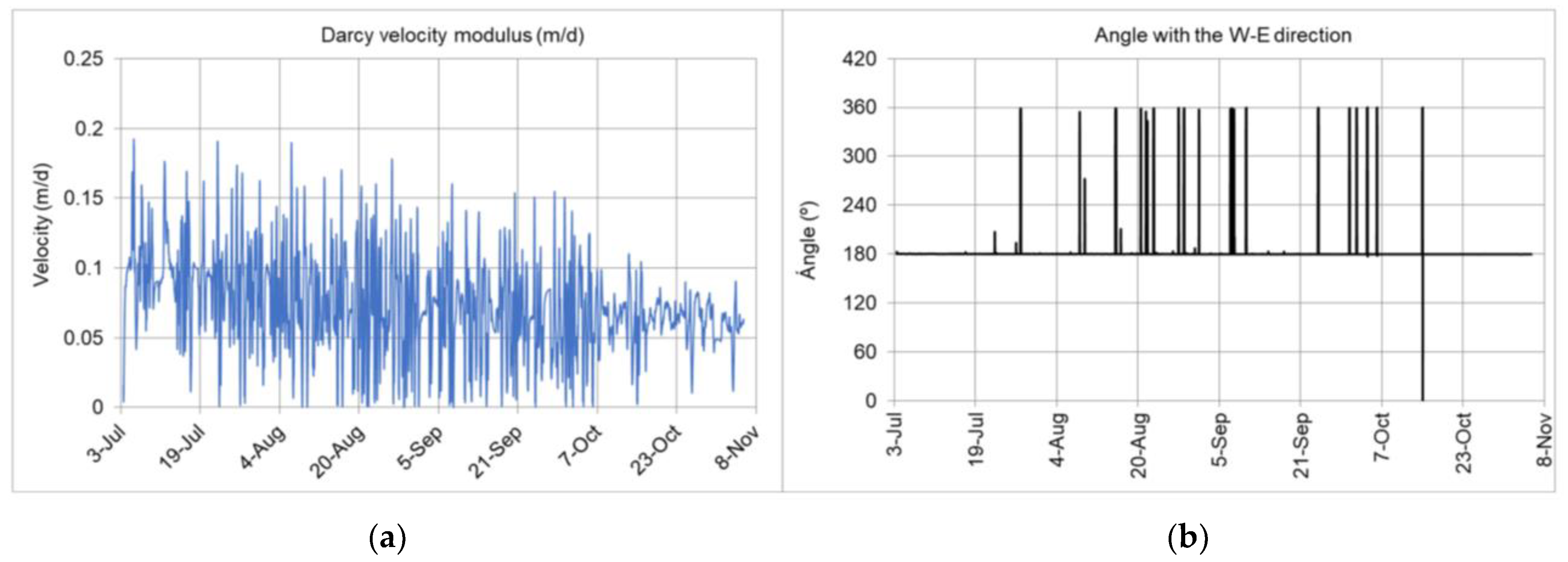
• The computed Darcy velocity in the gravel layer ranges from 15 to 30 cm/d near the PS26 borehole (near the reservoir), while the Darcy velocity at the PS16 borehole (further away from the reservoir) ranges from 1 to 10 cm/d. Darcy velocity in the shallow marls (FAD) is two to three orders of magnitude smaller than the velocity in the gravels.
• The model reproduces the vertical hydraulic head drop from the alluvial silts and to the sands and gravels layer at PS19 and PS5 boreholes. However, the computed heads in boreholes PS5E and PS5F exhibited smaller fluctuations than the measured hydrographs, which could be attributed to superficial inflows into the boreholes.
• The measured heads in the PS5F borehole between March and December 2021 remained almost constant, indicating that the hydraulic head was located below the bottom of the borehole, which maintained a water layer at the bottom.
• The recorded fluctuations in the measured heads within the S35 series boreholes are subject to notable uncertainties. These oscillations may potentially stem from various factors, including the infiltration of surface water into the borehole, which could be influenced by snow accumulation during winter months. The construction of a drain near the S35E borehole in April 2021 could have affected the measured heads. Consequently, there are significant uncertainties that warrant further investigation to enhance the model’s accuracy within this specific area.

These findings offer valuable insights into the understanding of the hydrodynamics and the hydrogeological evolution of the system as well as the quantification of the water and contaminant fluxes, enhances the confidence of the site managers on the conceptual model of the site, and helps to establish priorities in management options and resources to concentrate them to reduce main uncertainties. An improved understanding of the site should allow a better design and optimization of measures to protect groundwater quality. Numerical models are useful to support specific actions, simulate remediation alternatives, contribute to implement effective management strategies for landfill sites, and mitigate potential environmental risks associated with leachate migration.

The numerical model presented here could be improved with future research studies considering a detailed three-dimensional groundwater flow model of the landfill and a two-dimensional horizontal groundwater flow model for the entire Gállego River alluvial aquifer [33,37].

The methods, tools, and findings reported here for the Sardas landfill will also be useful for the study and design of remediation actions at other similar sites affected by HCH pollution in other places of Spain (Pontevedra and Vizcaya) and the rest of Europe (LINDANET) [14].

References

1. Grung, M.; Lin, Y.; Zhang, H.; Steen, A.O.; Huang, J.; Zhang, G.; Larssen, T. Pesticide Levels and Environmental Risk in Aquatic Environments in China—A Review. Environ. Int. 2015, 81, 87–97. [Google Scholar] [CrossRef] [PubMed]
2. Sun, J.; Pan, L.; Tsang, D.C.W.; Zhan, Y.; Zhu, L.; Li, X. Organic Contamination and Remediation in the Agricultural Soils of China: A Critical Review. Sci. Total Environ. 2018, 615, 724–740. [Google Scholar] [CrossRef] [PubMed]
3. Vijgen, J.; De Borst, B.; Weber, R.; Stobiecki, T.; Forter, M. HCH and Lindane Contaminated Sites: European and Global Need for a Permanent Solution for a Long-Time Neglected Issue. Environ. Pollut. 2019, 248, 696–705. [Google Scholar] [CrossRef] [PubMed]
4. Vijgen, J.; Yi-Fan, L.; Forter, M.; Lal, R.; Weber, R. The Legacy of Lindane and Technical HCH Production. Organohalog. Comp. 2005, 68, 899–904. [Google Scholar]
5. Wycisk, P.; Stollberg, R.; Neumann, C.; Gossel, W.; Weiss, H.; Weber, R. Integrated Methodology for Assessing the HCH Groundwater Pollution at the Multi-Source Contaminated Mega-Site Bitterfeld/Wolfen. Environ. Sci. Pollut. Res. 2013, 20, 1907–1917. [Google Scholar] [CrossRef] [PubMed]
6. Weber, R.; Watson, A.; Forter, M.; Oliaei, F. Review Article: Persistent Organic Pollutants and Landfills—A Review of Past Experiences and Future Challenges. Waste Manag. Res. J. Sustain. Circ. Econ. 2011, 29, 107–121. [Google Scholar] [CrossRef]
7. Lorenzo, D.; García-Cervilla, R.; Romero, A.; Santos, A. Partitioning of Chlorinated Organic Compounds from Dense Non-Aqueous Phase Liquids and Contaminated Soils from Lindane Production Wastes to the Aqueous Phase. Chemosphere 2020, 239, 124798. [Google Scholar] [CrossRef]
8. Ma, Y.; Yun, X.; Ruan, Z.; Lu, C.; Shi, Y.; Qin, Q.; Men, Z.; Zou, D.; Du, X.; Xing, B.; et al. Review of Hexachlorocyclohexane (HCH) and Dichlorodiphenyltrichloroethane (DDT) Contamination in Chinese Soils. Sci. Total Environ. 2020, 749, 141212. [Google Scholar] [CrossRef] [PubMed]
9. European Parliament; Directorate General for Internal Policies of the Union; Vega, M.; Romano, D.; Uotila, E. Lindane (Persistant Organic Pollutant) in the EU; European Parliament: Strasbourg, France, 2016; Available online: https://data.europa.eu/doi/10.2861/167592 (accessed on 9 August 2023).
10. Vijgen, J.; Abhilash, P.C.; Li, Y.F.; Lal, R.; Forter, M.; Torres, J.; Singh, N.; Yunus, M.; Tian, C.; Schäffer, A.; et al. Hexachlorocyclohexane (HCH) as New Stockholm Convention POPs—A Global Perspective on the Management of Lindane and Its Waste Isomers. Environ. Sci. Pollut. Res. 2011, 18, 152–162. [Google Scholar] [CrossRef]
11. Femina Carolin, C.; Kamalesh, T.; Kumar, P.S.; Rangasamy, G. An Insights of Organochlorine Pesticides Categories, Properties, Eco-Toxicity and New Developments in Bioremediation Process. Environ. Pollut. 2023, 333, 122114. [Google Scholar] [CrossRef]
12. Intisar, A.; Ramzan, A.; Sawaira, T.; Kareem, A.T.; Hussain, N.; Din, M.I.; Bilal, M.; Iqbal, H.M.N. Occurrence, Toxic Effects, and Mitigation of Pesticides as Emerging Environmental Pollutants Using Robust Nanomaterials—A Review. Chemosphere 2022, 293, 133538. [Google Scholar] [CrossRef] [PubMed]
13. Vijgen, J.; Fokke, B.; Van De Coterlet, G.; Amstaetter, K.; Sancho, J.; Bensaïah, C.; Weber, R. European Cooperation to Tackle the Legacies of Hexachlorocyclohexane (HCH) and Lindane. Emerg. Contam. 2022, 8, 97–112. [Google Scholar] [CrossRef]
14. European Regional Development Fund. LINDANET Final Report. 2023. Available online: https://projects2014-2020.interregeurope.eu/lindanet/library/#folder=3610 (accessed on 26 July 2023).
15. An, R.; Li, B.; Zhong, S.; Peng, G.; Li, J.; Ma, R.; Chen, Q.; Ni, J. Distribution, Source Identification, and Health Risk of Emerging Organic Contaminants in Groundwater of Xiong’an New Area, Northern China. Sci. Total Environ. 2023, 893, 164786. [Google Scholar] [CrossRef] [PubMed]
16. Fernández, J.; Arjol, M.A.; Cacho, C. POP-Contaminated Sites from HCH Production in Sabiñánigo, Spain. Environ. Sci. Pollut. Res. 2013, 20, 1937–1950. [Google Scholar] [CrossRef] [PubMed]
17. Santos, A.; Fernández, J.; Guadaño, J.; Lorenzo, D.; Romero, A. Chlorinated Organic Compounds in Liquid Wastes (DNAPL) from Lindane Production Dumped in Landfills in Sabiñanigo (Spain). Environ. Pollut. 2018, 242, 1616–1624. [Google Scholar] [CrossRef] [PubMed]
18. Zhan, L.; Wu, L.; Han, H.; Zhang, S.; Zhou, H.; Song, X.; Zhao, L.; Guo, Q.; Chen, Y. Hydrogeological Classification of Municipal Solid Waste Landfill Sites in China and Correlation with Groundwater Contaminant Migration. Hydrogeol. J. 2023, 31, 771–787. [Google Scholar] [CrossRef]
19. Casado, I.; Mahjoub, H.; Lovera, R.; Fernández, J.; Casas, A. Use of Electrical Tomography Methods to Determinate the Extension and Main Migration Routes of Uncontrolled Landfill Leachates in Fractured Areas. Sci. Total Environ. 2015, 506–507, 546–553. [Google Scholar] [CrossRef]
20. EMGRISA. Servicio de Seguimiento Hidrogeológico de Sardas, Sabiñánigo (Huesca) 2013–2014. Informe de Elaboración de Modelo de Simulación de Flujo de La Parcela al Pie de Vertedero y Zonas Aledañas, 2014. Technical Report. Unpublished work.
21. Samani, S.; Moghaddam, H.K.; Zareian, M.J. Evaluating Time Series Integrated Groundwater Sustainability: A Case Study in Salt Lake Catchment, Iran. Environ. Earth Sci. 2021, 80, 603. [Google Scholar] [CrossRef]
22. Samani, S.; Vadiati, M.; Nejatijahromi, Z.; Etebari, B.; Kisi, O. Groundwater Level Response Identification by Hybrid Wavelet-Machine Learning Conjunction Models Using Meteorological Data. Environ. Sci. Pollut. Res. Int. 2023, 30, 22863–22884. [Google Scholar] [CrossRef]
23. Julià, X.; González, G.; Alonso, M. Estudio Batimétrico y de Caracterización de Sedimentos Del Embalse de Sabiñánigo. URS. Technical Report for the Ebre River Water District. Zaragoza. 2009. Available online: https://www.chebro.es/documents/20121/55149/2009_Estudio_batimetrico_embalse_Sabinanigo.pdf (accessed on 29 August 2023).
24. Biosca, B.; Arévalo-Lomas, L.; Izquierdo-Díaz, M.; Díaz-Curiel, J. Detection of Chlorinated Contaminants Coming from the Manufacture of Lindane in a Surface Detritic Aquifer by Electrical Resistivity Tomography. J. Appl. Geophys. 2021, 191, 104358. [Google Scholar] [CrossRef]
25. CHE. Análisis Ambiental de Los Sedimentos y Del Entorno Del Embalse de Sabiñánigo (Huesca) y Evaluación de Riesgos. 2010. Available online: https://www.chebro.es/documents/20121/55149/03_evaluacion_riesgos.pdf (accessed on 2 September 2023).
26. Descontaminación Integral del Lindano. Portal de Aragon. Available online: https://www.aragon.es/-/descontaminacion-integral-lindano (accessed on 4 September 2023).
27. Environmental Problem Caused by the Presence of Lindane in Sabiñanigo. Company for the Management of Industrial Waste-Emgrisa. Available online: http://emgrisa-original.versionesbeta.com/project/seguimiento-y-control-del-riesgo-medio-ambiental-en-vertedero-de-sardas/ (accessed on 4 September 2023).
28. Espinha Marques, J.; Samper, J.; Pisani, B.; Alvares, D.; Carvalho, J.M.; Chaminé, H.I.; Marques, J.M.; Vieira, G.T.; Mora, C.; Sodré Borges, F. Evaluation of Water Resources in a High-Mountain Basin in Serra Da Estrela, Central Portugal, Using a Semi-Distributed Hydrological Model. Environ. Earth Sci. 2011, 62, 1219–1234. [Google Scholar] [CrossRef]
29. Samper, J.; Xu, T.; Yang, C. A Sequential Partly Iterative Approach for Multicomponent Reactive Transport with CORE2D. Comput. Geosci. 2009, 13, 301–316. [Google Scholar] [CrossRef]
30. Águila, J.F.; Montoya, V.; Samper, J.; Montenegro, L.; Kosakowski, G.; Krejci, P.; Pfingsten, W. Modeling Cesium Migration through Opalinus Clay: A Benchmark for Single- and Multi-Species Sorption-Diffusion Models. Comput. Geosci. 2021, 25, 1405–1436. [Google Scholar] [CrossRef]
31. Águila, J.F.; Samper, J.; Pisani, B. Parametric and Numerical Analysis of the Estimation of Groundwater Recharge from Water-Table Fluctuations in Heterogeneous Unconfined Aquifers. Hydrogeol. J. 2019, 27, 1309–1328. [Google Scholar] [CrossRef]
32. Cousquer, Y.; Jourde, H. Reducing Uncertainty of Karst Aquifer Modeling with Complementary Hydrological Observations for the Sustainable Management of Groundwater Resources. J. Hydrol. 2022, 612, 128130. [Google Scholar] [CrossRef]
33. Sobral, B.; Samper, J.; Pisani, B.; Guadaño, J.; Gómez, J. Quantifying Groundwater Flow and Dissolved HCH Transport at the Sardas Landfill Using a 3D MODFLOW Model in Sabiñánigo, Spain. Civil Engineering School. Interdisciplinar Center for Biology and Chemistry (CICA). Universidade de A Coruña. Campus de Elviña, 15071, A Coruña, Spain. 2023; manuscript in preparation. [Google Scholar]
34. Krause, P.; Boyle, D.P.; Bäse, F. Comparison of Different Efficiency Criteria for Hydrological Model Assessment. Adv. Geosci. 2005, 5, 89–97. [Google Scholar] [CrossRef]
35. Elshall, A.S.; Arik, A.D.; El-Kadi, A.I.; Pierce, S.; Ye, M.; Burnett, K.M.; Wada, C.A.; Bremer, L.L.; Chun, G. Groundwater Sustainability: A Review of the Interactions between Science and Policy. Environ. Res. Lett. 2020, 15, 093004. [Google Scholar] [CrossRef]
36. Jafarzadeh, A.; Khashei-Siuki, A.; Pourreza-Bilondi, M. Performance Assessment of Model Averaging Techniques to Reduce Structural Uncertainty of Groundwater Modeling. Water Resour. Manag. 2022, 36, 353–377. [Google Scholar] [CrossRef]
37. Sobral, B.; Samper, J.; Mon, A.; Montenegro, L.; Pisani, B. Modeling the Impacts of Lindane Contamination on Alluvial Aquifers and Their Interaction with a Reservoir in Sabiñánigo, Spain. Civil Engineering School. Interdisciplinar Center for Biology and Chemistry (CICA). Universidade de A Coruña. Campus de Elviña, 15071, A Coruña, Spain. 2023; manuscript in preparation. [Google Scholar]
Figure 1. Flowchart of the methodology used for constructing the numerical model of the Sardas site.
Water 15 03457 g001
Figure 2. Location of the study site. The map shows the trace of the A-A’ vertical profile along the thalweg of the former gully and through the Gállego River alluvial until the Sabiñánigo reservoir.
Water 15 03457 g002
Figure 3. Evolution of the vertical profile of the study site used by EMGRISA and the Government of Aragon to define the conceptual model of the site since the 1950s to its current state.
Water 15 03457 g003
Figure 4. Map of the site showing the trace of the E–W hydrogeological profile and the location of the boreholes considered for the model along the vertical profile.
Water 15 03457 g004
Figure 5. Model domain and material zones identified with different colors for each hydrogeological material zone (upper plot). The colors of the zones are listed in Table 2. A material zone is a made of all the triangular elements having the same hydraulic conductivity values. The intermediate and bottom plot show zooms of the western and eastern parts of the model domain with the 2D grid of triangular finite elements and boundary conditions.
Water 15 03457 g005
Figure 6. Infiltration recharge time function in the alluvial, N-330 embankment, and Sardas landfill wastes: (a) between January 2013 and September 2022; (b) between 3 July and 5 November 2018.
Water 15 03457 g006
Figure 7. Inflow through the surrounding marly rock at the head of the Sardas landfill time function: (a) between January 2013 and September 2022; (b) between 3 July and 5 November 2018.
Water 15 03457 g007
Figure 8. Inflow through the perimeter ditches time function: (a) between January 2013 and September 2022; (b) between 3 July and 5 November 2018.
Water 15 03457 g008
Figure 9. Time evolution of the Sabiñánigo reservoir water level: (a) between January 2013 and September 2022; (b) between 3 July and 5 November 2018.
Water 15 03457 g009
Figure 10. Time function of the pumped flow rate in borehole S37 drilled in the landfill wastes just upstream the front slurry wall: (a) between January 2013 and September 2022; (b) between 3 July and 5 November 2018.
Water 15 03457 g010
Figure 11. Contour plots of computed hydraulic heads along the vertical profile. Colored zones correspond to material zones. The upper plot shows the results for the western part of the profile in the Gállego River alluvial (contour interval equal to 1 m) and the lower plot shows the results in the eastern part of the profile (contour interval equal to 2 m).
Water 15 03457 g011
Figure 12. Measured and computed hydraulic heads from January 2013 to September 2022 in boreholes drilled in the alluvial (upper left plot), gravels and silts (upper right and lower left plots), and in the N-330 road embankment (lower right plot).
Water 15 03457 g012
Figure 13. Measured and computed hydraulic heads downstream and upstream the front slurry wall (upper left plot), in the landfill wastes along the thalweg of the former gully (upper right plot) and at the head of the landfill (lower plot) from January 2013 to September 2022.
Water 15 03457 g013
Figure 14. Measured and computed hydraulic heads of boreholes screened either in gravels or in silts for the following periods: From 3 July 2013 to 8 November 2018 (upper plots) and from 1 October to 8 October 2018 (bottom plot).
Water 15 03457 g014
Figure 15. Time evolution of groundwater Darcy velocity through the sands and gravels near borehole PS26: (a) velocity modulus; and (b) angle of the velocity vector with respect to the W–E direction.
Water 15 03457 g015
Figure 16. (a) PS26 measured hydraulic head and Sabiñánigo reservoir water level in the left vertical axis and groundwater flow direction in the right vertical axis between the 3rd and the 8th of September 2018; (b) enlargement on the 7 September 2018.
Water 15 03457 g016
Figure 17. Statistical plots of hydraulic head residuals (differences between computed and measured heads): (a) sample histogram; (b) quantile-quantile (q-q) plot.
Water 15 03457 g017