1. Introduction
Human progress has recently experienced a significant acceleration, which has led to notable changes in land cover and climate [
1]. The climate and LULC changes have the potential to have a domino effect on many different aspects, such as crop productivity, hydropower generation, and the hydrological cycle [
2,
3]. Global warming is to blame for the harsh climatic and weather conditions [
4,
5]. The Intergovernmental Panel on Climate Change (IPCC) concluded that greenhouse gas (GHG) emissions from the actions of humans have increased to previously unheard-of levels, which is causing climate change. These emissions, considered the highest ever recorded, have a significant impact on meteorological parameters [
6,
7]. The temperature of Earth has risen by 0.85 °C between 1880 and 2012, and this increase has been accompanied by changes in precipitation patterns. These variations in precipitation and temperature are a result of the environment’s increasing GHG concentration. Changes in temperature and precipitation have a direct effect on quantity, speed, and hour of the peak river flow [
8]. Along with other essential aspects of the flow regime, these modifications also have an impact on peak and baseline flow dynamics [
9]. The hydrological cycle is significantly affected by changes in climate and LULC [
10,
11].
Diverse LULC conditions lead to variations in the losses encountered during precipitation–runoff events. Evaporation, interception, evapotranspiration, infiltration, transpiration, and watershed leakage are only a few of the factors that make up these losses. Various LULC scenarios show various loss patterns in the transformation of rainfall into runoff events [
12]. According to Rahman [
8], the variations in losses brought on by different LULC conditions have an impact not only on the total amount of runoff produced during rainfall events but also on flow velocity and the amount of time that it takes for surface water flow to reach its peak. The exponential growth of the population has a notable impact on land conversion, particularly the transformation of forested areas into non-forest or agricultural zones [
13,
14,
15]. Therefore, it is essential to put into practice appropriate planning techniques for climate as well as land use variations to increase the catchment regions’ capacity to sustain water supplies, meet a variety of needs, and eventually benefit the larger community.
Researchers have been actively involved in measuring each impact on the availability of water and flow characteristics in order to understand how these factors affect them. Individual studies [
9,
16,
17,
18,
19,
20,
21] have looked into the consequences of LULC changes. Similar to this, a few studies [
22,
23,
24,
25] have concentrated on examining the influence of changing climate on runoff. However, there has not been much discussion on the combined influence of CC and LULC in the literature [
8,
26,
27,
28,
29,
30,
31,
32].
The hydrological system and a variety of linked operations, including the generation of hydroelectricity, the management of water resources, and tourism-related activities, depend heavily on mountainous watersheds [
33]. The assessment of climate change and land use/land cover change impacts on water resources within a catchment is of paramount importance in contemporary environmental research. This multifaceted examination is indispensable for comprehending the intricate dynamics that underlie water resource availability and quality. It plays a pivotal role in developing strategies for sustainable water management, conservation, and adaptation, particularly in regions grappling with escalating environmental uncertainties. However, despite its critical relevance, there exists a notable research gap in this domain, with a limited number of comprehensive studies conducted to date. This research gap underscores the urgency of further exploration and investigation in order to fill critical knowledge voids and inform evidence-based decision making for the preservation and efficient utilization of water resources in the face of evolving climate and land use patterns. Particularly, the Kunhar River basin in Pakistan’s north has significant hydropower, water resource, and tourism potential [
2]. As a result of the Kunhar river basin’s major contribution to the water, energy, agriculture, and tourist industries in Pakistan, this study concentrates on this. In the Kunhar river basin, only a limited number of studies [
24,
34,
35] have observed the influence of CC on stream flows. Noteworthy is the fact that no earlier research has been performed to evaluate the combined effects of climatic and LULC changes on discharge in this basin. The Sustainable Development Goals (SDGs) are directly line with the goals of this research, especially SDG 6.6.1, which deals with the evolution of water-related ecosystems. Additionally, it helps with the assessment of land degradation in relation to overall land coverage (SDG 15.3.1) and the incorporation of climate change measures into initiatives, plans, and planning (SDG 13.2) [
36,
37].
In this research, several hypotheses were posited to guide our investigation into the impacts of climate change and land use/land cover changes on water resources within the Kunhar River basin. Firstly, it was hypothesized that the basin will undergo alterations in its hydrological regime, including changes in precipitation patterns, increased temperatures, and shifts in runoff events as climate change intensifies. Secondly, evolving land use and land cover patterns within the catchment are expected to impact both the quantity and quality of water resources, influencing surface and groundwater availability. It was further hypothesized that these combined effects of climate change and land use changes will challenge the sustainability of water resources in the Kunhar River basin, potentially affecting water availability for various purposes. Additionally, ecological consequences were anticipated, with impacts on aquatic habitats, biodiversity, and overall ecosystem health. Lastly, it was hypothesized that our integrated assessment of these impacts will provide invaluable insights for policy makers, resource managers, and local communities, facilitating the development of effective strategies for resilient water resource management and conservation in the face of ongoing environmental changes.
The objectives of this study were established in light of the knowledge gap that exists and the importance of this study in relation to various Sustainable Development Goals (SDGs) are as follows: (a) to investigate the LULC temporal variations across KRB, (b) to examine the influence of both LULC alterations and CC on KRB’s streamflow. To accomplish these goals, two distinct land cover maps were examined using Arc GIS 10.5 software, and the impact of LULC modifications on streamflow was evaluated using the SWAT model. Hydro-climatic data from various sources were compiled using the SWAT model to investigate influence of CC on stream flows. The devoted section contains a thorough explanation of methodology, while section on hydrological modelling contains thorough information about the hydrological model used.
2. Materials and Methods
2.1. Study Area
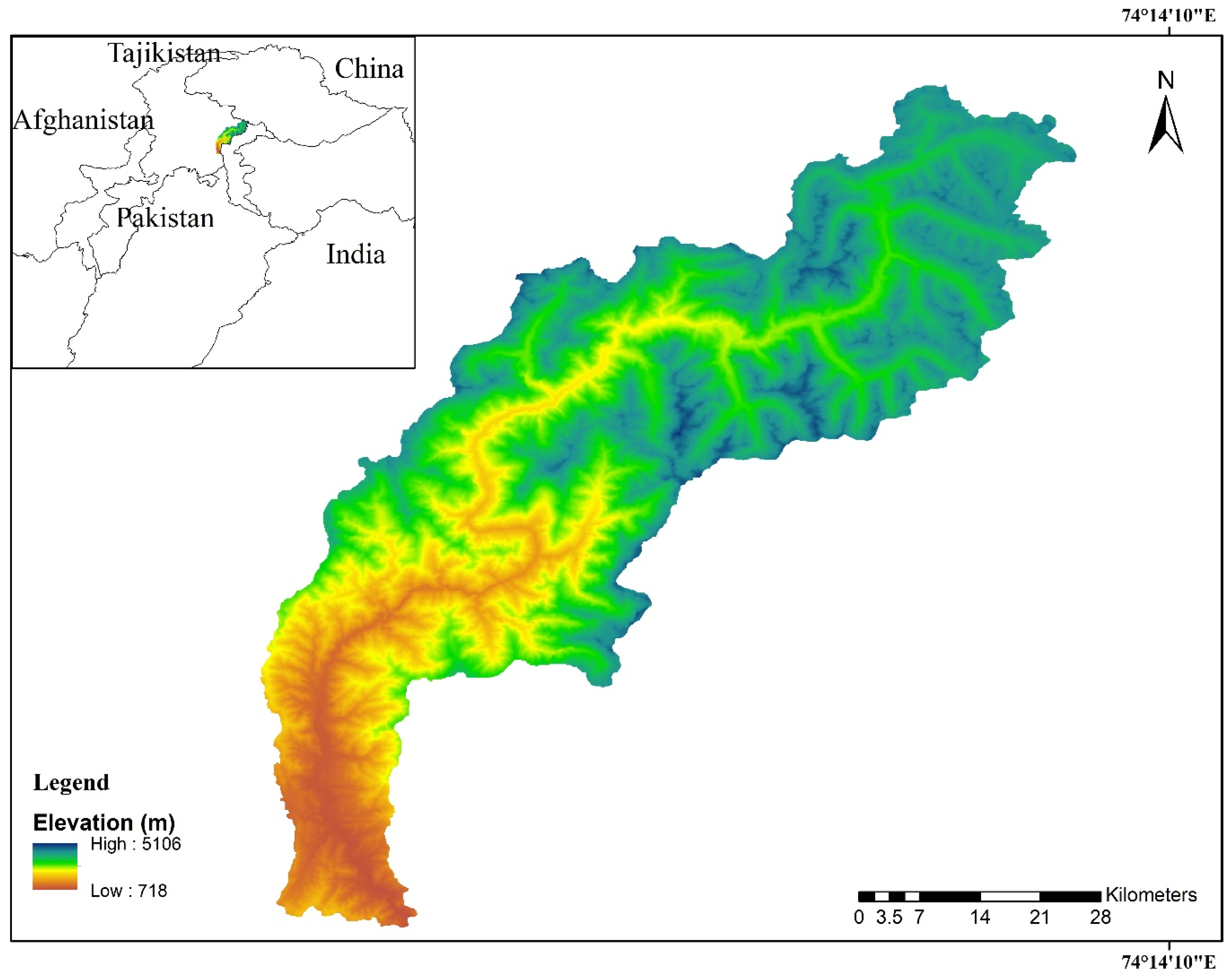
The geographical coordinates of Kunhar watershed covering an area of approximately 2359 km
2 are displayed in
Figure 1. The river originates from the Babusar Top and eventually joins the River Neelam [
38]. The Kunhar River’s main stretch extends for 141 km till it reaches Ghari Habibullah. The elevation map of the basin, as illustrated in
Figure 1, demonstrates a significant elevation difference between the lowest and highest points, amounting to approximately 4388 m. The Kunhar watershed has a slope that varies from the basin’s average slope of about 53% to other slope characteristics.
The Kunhar River basin, located in Pakistan, is a region of remarkable geographical and hydrogeological diversity. The Kunhar basin is located in a humid, subtropical zone. In the present study, hydro-climatic data were processed for the period of 1961–2000 to extract some basic information about the hydro-climatic conditions in the basin. The average annual temperature in the basin is about 13 °C (2–23 °C). February is the coldest and July is the warmest month here. This was calculated from the data of the Naran and Balakot climate stations available for the period of 1961–2000. At Balakot, located in the lower part of basin, minimum temperature ranges from 2 °C (January) to 23 °C (July) and maximum temperature from 14 °C (January) to 35 °C (June). At Naran, located in the upper part of the basin, minimum temperature ranges from −9 °C (February) to 13 °C (July) and maximum temperature from −1 °C (February) to 23 °C (July). The Kunhar basin has an annual precipitation of about 1500 mm with two peaks. The first peak occurs in the upper part of the basin in the month of March because of the Western Disturbances (WDs) system in winter. Most parts of Pakistan, and its northwestern parts primarily, obtain precipitation due to WDs. WDs are caused by depressions over Mediterranean regions, resulting in precipitation over central and southwest Asia in the months of December to March. The second peak happens in the month of July and in the lower parts of the basin due to the summer monsoons, which are the result of the saturated south western winds from the Bay of Bengal and Arabian Sea. It can be concluded that the monsoons do not reach the upper part of the basin, although WDs affect the whole basin. On the other hand, there is only one big streamflow peak, both in the upper (Naran) and lower parts (Gari Habibullah) of the basin, that occurs in the month of July. This means the precipitation from December to March (winter) accumulates as snow cover, especially in the upper parts of the basin, and then starts melting after March and lasts till July when it overlaps with monsoon precipitation and results in one big peak. An average flow of about 1350 mm (103 m3/s) has been measured at Gari Habibullah near the mouth of the basin for the period of 1961–2000.The topography of the basin is equally striking, with the northern portion dominated by the towering Himalayan and Karakoram mountain ranges, including the imposing Nanga Parbat, which stands at an elevation of 8126 m. This mountainous region is the source of numerous tributaries, glaciers, and snowfields that feed into the Kunhar River. As one ventures southward, the terrain gradually becomes less steep, giving way to fertile valleys and plateaus that are conducive to agriculture and human settlement.
In terms of hydrogeology, the Kunhar River basin’s complexity is influenced by its geological diversity. The basin comprises a mosaic of sedimentary, metamorphic, and igneous rock formations. This geological heterogeneity results in a multifaceted aquifer system, with groundwater storage and flow patterns varying across the basin. Geological fault lines and fractures further complicate the movement of groundwater. A significant hydrological feature is the presence of glaciers in the upper reaches of the basin. These glaciers, which melt during the warmer months, contribute substantially to the flow of the Kunhar River and its tributaries, impacting the basin’s overall hydrology. Together, these factors make the Kunhar River basin an intriguing area of study for assessing the effects of climate change and land use/land cover changes on its valuable water resources, given its dynamic environment and wealth of geological and hydrological data.
2.2. Dataset
2.2.1. Soil Classification
The input of soil classifications is regarded as an essential component for building the hydrological model (SWAT). The model depends on a number of soil surface parameters, including texture, biochemical potentials, and physical features including hydraulic conductivity, bulk density and available moisture content (AMC). The soil map of Kunhar basin was created using IPCC Global Soil Classification dataset. There are four major soil types in the basin, with Gleyic Solonchaks making up the majority (76%) of the basin’s surface.
Figure 2 shows spatial distribution of soil categorization has been produced using the SWAT model.
Table 1 and
Figure 2 provides more information on these soil classes, particularly their given names and distribution across the study area.
2.2.2. GCM-Based Climate Data
The CMIP6 was utilized to gather the precipitation (Pr), minimum temperature (T
min) and maximum temperature (T
max) data for four GCMs with respect to SSP2 and SSP5 scenarios. The outputs from the chosen GCMs were then downscaled to enable analysis at a similar resolution, notably at river basin magnitude, this is used for projected precipitation and temperature. Following methods was used by Babur et al. [
23]. The selection of GCMs considered elements such as spatial accuracy, era, validity, and representation of simulations. Out of the initial four GCMs used for this study. One GCM was chosen because of its superior performance in accurately simulating temperatures and precipitation for baseline time frame of 1985–2015. To determine best method for downscaling temperature and precipitation data, various statistical downscaling strategies were examined. The Kunhar River Basin’s future flows were subsequently modelled using the chosen approach. The selected GCMs supplied the simulated climatic variables for two distinct intensities: medium (SSP2) and high (SSP5), including T
min, T
max and Pr. Detailed review of GCMs used in present investigation is provided in
Table 2. The low radiation forcing scenario (SSP1) was excluded from this investigation. It is difficult to achieve a considerable and rapid decrease in greenhouse gas emissions given the degree of industrialization, which makes it difficult to meet the aforementioned mitigation scenario [
39]. Instead, the extremely high radiation forcing scenario (SSP5) and the medium stabilization forcing scenario (SSP2) were taken into account. For the time period covering 1985 to 2100, projected climate parameters based on the chosen GCMs under SSP2 and SSP5 were obtained. The baseline era of 1985 to 2014 and the future period of 2015 to 2100 were used to divide this time period into two separate halves.
2.3. Methodology
The methodology adopted in this study refers to specific approach or set of procedures used to collect and analyze data, conduct experiments, or explore a research question. The accompanying
Figure 3 provides a visual representation of the methodology flowchart, outlining the step-by-step sequence and activities involved in this study’s methodology.
2.3.1. Statistical Downscaling
In order to address bias between temperature and precipitation forecasts obtained from four different models with respect to the SSP2 and SSP5 scenarios, CMhyd model was utilized to supply bias correction at the river basin scale [
39,
40]. CMhyd model has successfully been applied in numerous places across the globe by successfully bridging the gaps between observed climate variables collected from gauges and simulated data based on GCMs [
41]. Anandhi et al.’s [
41] hydro-climatological research at the river basin scale has shown CMhyd model to be a trustworthy and dependable method for downscaling GCM results. The CMhyd model offers numerous statistical downscaling techniques for temperature and precipitation. In this investigation, under the constraints of SSP2 and SSP5, these various techniques were used to downscale GCM results for future time frame spanning from 2015 to 2100. This was carried out by merging predicted estimates from the GCMs with information on daily precipitation, maximum temperature, and lowest temperature that was gathered during baseline period of 1985 to 2014.
2.3.2. The SWAT Model’s Description and Setup
The SWAT was used in this work to project river discharge according to influence of both climate change and land cover. The SWAT is a hydrological model with a physical foundation that uses a framework with semi-distributed parameters [
41,
42]. This model has ability to simulate and evaluate influence of CC and land management practices on a variety of hydrological parameters, such as river water quality, discharge and sediment production, across basins of varied sizes [
43]. The main channel is connected to each of the sub-catchments that the SWAT splits a river basin into. The smallest unit within the basin is a Hydrological Response Unit (HRU) in the SWAT, which is based on a combination of soil type, slope, and land cover. The SWAT’s capacity to figure out inputs from snowfall and melting glaciers utilizing the TIA (temperature index algorithm) is one of its computational strengths. This method, which splits watersheds into several elevation zones, works well for modelling the hydrological consequences of watersheds characterized by snow and glaciers. The SWAT enables a more thorough portrayal of the hydrological procedures inside the model by further dividing elevation of each of the sub-catchment into ten zones. A number of academics have used the TIA to simulate flow rates in glaciated watersheds in the past. Here are a few examples: Babur et al.’s [
23] study in Jhelum River basin (Himalayan Region), Garee et al.’s [
44] study in Hunza River basin (Karakoram Region), and Zhang et al.’s [
45] study in Yellow River source area (Tibetan Plateau). Similar to that, the TIA technique was used in our work to calculate how much meltwater contributed to the total river flow. The study region was separated into 10 elevation zones for each subbasin, allowing for estimating the amount of P
r, T
max and T
min for every region using the lapse rate method. The SWAT model incorporates a number of evapotranspiration (ET) estimation methods, including the Priestley- Hargreaves, Taylor and Penman-Monteith approaches. This study estimated ET using the Hargreaves approach. The terrain/topography data, climate data (such as P
r, T
max, T
min, wind speed, solar radiation and relative humidity), soil characteristics, land cover information, and land-use management data are all necessary input parameters for the SWAT model to run [
46]. According to earlier studies [
43,
46,
47], the SWAT has been widely used to successfully mimic hydrological and landscape dynamics at a worldwide scale. The SWAT model incorporates the WXGEN weather generator model [
48,
49], which could produce meteorological data or fill up any empty spots in the observations. In this study, the Kunhar River basin’s river discharge was simulated using the SWAT model with respect to two different scenarios: (a) present LULC and future CC, and (b) both future LULC and CC. Digital Elevation Model (DEM) with a spatial scale of 90 m, acquired using the SRTM (Shuttle Radar Topographic Mission), was used to build the river stream network and basin delineation. Based on changes in land cover and soil type, the KRB was divided into three sub-basins, resulting in 71 Hydrological Response Units (HRUs). Each sub-catchment was further separated into 10 elevation bands to account for orographic influences on precipitation and temperature data. The WXGEN weather generator was used to simulate prospective weather conditions, including wind speed (WS), sun radiation (SR), and relative humidity (RH), using the methods described in the reference [
50].
2.3.3. Calibration and Validation of the SWAT Model
The SWAT Calibration and Uncertainty Programme (SWAT-CUP) was utilized to calibrate and validate model using procedure outlined in Garee et al.’s [
44] study. The model’s performance and parameters were assessed for uncertainty using the SWAT-CUP’s Sequential Uncertainty Fitting (SUFI-2) approach. During model calibration process, the SWAT-CUP programme was run 10,000 times to determine the sensitive parameters for the hydrological model. In order to compare simulated results with observed data, the monthly flow data collected over the Ghari Habibullah gauge station were used as calibration time frame from 2001 to 2007. After that, observable data from 2008 to 2014 were used to validate the model.
2.3.4. Evaluating the Performance of Model
A number of assessment indicators, such as the PBIAS (percentage of bias), R
2 (coefficient of determination), and NSE (Nash-Sutcliffe efficiency), were used to gauge the SWAT model’s efficacy [
51]. Higher values suggest greater concordance with both simulated and observed findings. The R
2 value can range from −1 to 1. These assessment measures were used to gauge the accuracy and dependability of the model-simulated outcomes offered by the hydrological model. NSE, a performance evaluating indicator with a range of 0–1, indicates how well the simulated and observed data agree. Higher figures indicate better agreement. Values greater than 0.50 are typically regarded as acceptable, indicating a reduced amount of simulation error [
52]. The percent bias (PBIAS), on the other hand, is a different evaluation metric that gauges the typical propensity of the values that are simulated to depart from what has been observed. Acceptable PBIAS levels typically range from −15% to +15%, suggesting that the simulation results are biased only slightly [
43]. The R
2 and NSE equations are shown below:
where,
,
,
, and
stand for simulated flows, measured flows, mean measured flows, and mean simulated flows, accordingly.
2.3.5. Present Land Cover Maps and Future Land Cover Projections
The current research examined expected and present land cover trends. Landsat imagery has already been used to produce maps of land cover for the years 2000, 2010, and 2022. Then, in order to track changes throughout the specified years, a plot of the regions included within every category of land cover was created. Maps were made to analyze patterns and use as inputs for the SWAT model, combining future land cover conditions with projected climatic conditions. Projected land use maps were simulated using TerrSet, especially the Land Change Modeller (LCM). In the present research, a combined Markov and Cellular Automata (CA) method known as CA Markov was used to estimate variations in land cover for the years 2040, 2070, and 2100. The Markov and CA Markov modules were employed in two steps of the modelling procedure to run the model and produce the simulated maps of land cover.
2.3.6. Markov Chain Analysis
Markov Chain Analysis (MCA) is a predictive modeling technique that utilizes historical data to forecast future land use changes. It is a stochastic modeling procedure that provides insights into likelihood of land use transitions with respect to the measured data from past time frames. The odds of cells changing from present land cover class to the next during a given time frame are calculated using MCA whenever used for a geographic region divided into cells representing various land use classes. These transition probabilities help us comprehend how circumstances might alter throughout time. By measuring projected pixel changes and the chances of one land cover class switching to another, MCA develops a transition matrix [
53]. A Markov transformation grid P can be written as shown below:
where,
= the first and second time periods’ land cover types,
= Probability of transitioning from one land cover class to another. After a given number of time units, a set of conditionally probable maps called transitional potential pictures were produced. These maps display the probabilities of every kind of land cover in a certain pixel. It is important to note that Markov analysis does not consider reasons behind land-cover changes. Additionally, one limitation of Markov analysis is its lack of spatial sensitivity, as it does not account for geographical context. To address this limitation, cellular automata were employed to introduce a spatial component the modelling procedure.
2.3.7. CA_MARKOV
To project the future land cover image, Cellular Automata and the integrated CA-MARKOV component within the TERRSET package were coupled. The CA-MARKOV model combines methods of Markov Chain, Cellular Automata, Multi-Objective Land Allocation (MOLA) and Multi-Criteria. The Markov chain analysis may now take into account geographical contiguity and information about the expected geographic spread of land use shifts thanks to this integration. The algorithm functions as follows: The transition file contains the projected changes in LULC from every present class to every other class in the upcoming time period, which were computed using a Markov Chain evaluation of two land cover maps from past. The latter land cover image, which was used for Markov Chain analysis, is used as the base of operations for the alteration projection utilizing the initial land cover image. To assess a pixel’s inherent suitability for different types of land cover, appropriateness or transition maps are utilized. These maps apply weights based on characteristics such as proximity to existing places with a certain land cover class. A contiguity filter is typically used to down weight pixels that are situated far from current boundaries of that class in favor of contiguous appropriate areas.
3. Results
3.1. Downscaling Future Climate Data
GCMs are intricate numerical depictions of the planet’s climate and its plethora of linkages [
54]. To create grid-like compartments in the atmosphere, often with a spatial resolution of 100–200 km. Within each grid, equations that describe atmospheric dynamics are solved. This coarse resolution, however, may result in inaccurate simulations of some significant physical processes and climatic phenomena. Bias correction methods must therefore be applied in order to improve dependability and precision of downloaded GCM data.
3.2. Selection of the GCM
This coarse resolution, however, may result in inaccurate simulations of some significant physical processes and climatic phenomena. Therefore, in order to increase dependability and precision of downloaded GCM data, bias correcting techniques must be used.
Choosing a GCM for a study often entails taking into account a number of variables, including resolution, data accessibility, results from previous research, and performance metrics. Four fundamental techniques were used to choose the GCMs for the present investigation based on these features. By contrasting historical GCM data with actual ground data collected at the Balakot station, statistical measures including the R2 (coefficient of determination), MAE (mean absolute error) and RMSE (root mean square error) were used to assess performance of the chosen GCMs. The effectiveness of four CMIP6 GCMs at Balakot station is displayed in the tables below.
According to an analysis of the R
2, NSE, and RMSE values shown in
Table 3,
Table 4 and
Table 5, the performance of the climate simulation model “MPI-ESM1” was comparatively better. As a consequence, it was chosen as a climate simulation tool to evaluate potential changes in the region under study’s climate. This study concentrated on climate projections for the years 2015 to 2100, specifically those for precipitation, minimum temperature, and maximum temperature from the MPI-ESM1 model with respect to two distinct SSP2 and SSP5. To ensure accurate representation, bias adjustment using the CMhyd has been applied to each dataset.
3.3. Selecting Bias Correction Methods
Modelling data are observed at a large scale, GCMs often perform well, but when examined at the basin level, they frequently exhibit significant biases. The variance, quantiles and mean of model’s time-series parameters are to be adjusted by applying specified correction factors as part of the bias correction strategy. This adjustment seeks to reduce the bias at the scale of the basin by bringing the corrected model data series nearest to the observed variable. Five correction methods for precipitation and four correction methods for temperature were examined in
Table 6 to find the best downscaling method for the downloaded GCM data. These methods were used to adjust the temperature and precipitation data from Balakot station. Following that, a time-series analysis was used to assess each strategy’s efficacy, illustrated in
Table 7 and
Table 8.
It was shown after analyzing the performance metrics that all bias correction techniques considerably enhanced the raw GCM simulations. The adjustments of monthly averages for precipitation as well as temperature was achieved by the execution of these procedures. The “Distribution Mapping” strategy outperformed the others in terms of temperature correction, whereas the “Power Transformation” technique produced the best outcomes for precipitation. Using these techniques, the variability of the raw GCM simulations was successfully decreased, and the median was brought closer to the actual data.
3.4. Projected Variations in the Temperature and Precipitation
Projected data were downscaled to cover the full 21st century until the year 2100 after the relevant GCMs and downscaling methods for Pr, highest and lowest temperature were selected. The baseline period, which included years 1985 to 2014, and the future scenarios, which encompassed the years 2015 to 2100 under SSP2 and SSP5 scenarios, were created as two independent datasets for the projected precipitation and temperature.
3.5. Projection of Mean Maximum Temperature
By examining downscaled estimations of GCMs at both the annual and seasonal scales, involving winter, spring, summer, and autumn, the future of maximum temperature (T
max) were assessed. Based on results in
Table 9, it was concluded that SSP2 scenario would result in a rise in T
max of KRB of 14.3%, from 18.3 °C during the baseline time period of 1985–2014 to 20.9 °C in future time frame of 2015–2100. Additionally, the increase in T
max, from 18.3 °C to 22.1 °C in the direr SSP5 scenario, is anticipated to be 20.5%.
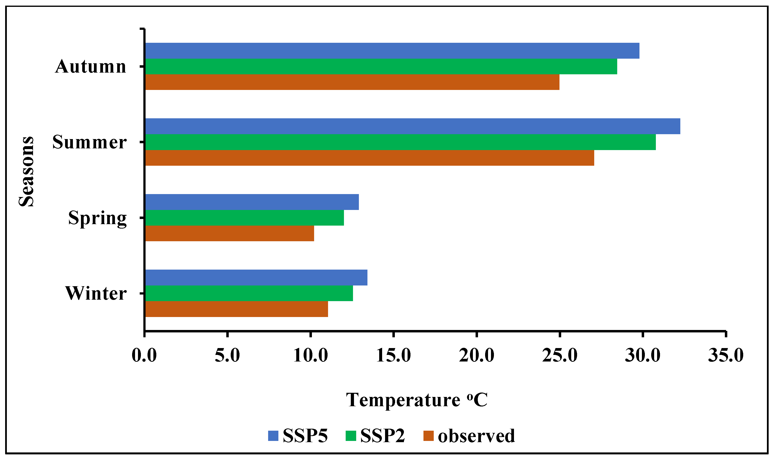
As shown in
Figure 4, the examination of temperature change was performed on a seasonal basis, comprising spring, winter, fall and summer. The findings show that the mean maximum temperature has risen during each of the four seasons. With a rise of 26.4% from 10.2 °C throughout the baseline era to 12.9 °C in the SSP5 scenario, the spring season shows the largest increase (
Figure 4). The average maximum temperature during the spring season increases by 17.5% in the SSP2 scenario, from 10.2 °C to 12 °C (
Figure 4). The summer season showed the least rise in the average maximum temperature, rising by 13.8% under the SSP2 scenario from 27.1 °C to 30.8 °C and by 19.2% under the SSP5 scenario from 27.1 °C to 32.2 °C (
Figure 4). Similar to how the maximum temperature increased in the winter and autumn seasons in SSP2 and SSP5 scenarios, with greater magnitudes shown in the SSP5 scenario. In the SSP2 and SSP5 scenarios, wintertime temperature increased by 13.6% and 21.4% from 11.1 °C to 12.6 °C and 13.4 °C, respectively. Additionally, as predicted by model, average maximum temperature rose by 13.9% and 19.3% in the autumn (
Figure 4).
3.6. Projected Mean Minimum Temperature
Future estimates from downscaled GCMs were examined at both the seasonal and annual scales to ascertain the likelihood of hydrological changes linked to T
min. Winter (December, January, and February), spring (March, April, and May), summer (June, July, and August), and autumn (September, October, and November) were all included in seasonal study. According to data in
Table 9, T
min in KRB rose by 20.9% under the SSP2 scenario, from 7.8 °C over the base period of 1985–2014 to 9.4 °C in future time frame of 2015–2100. With temperatures increasing from 7.8 °C to 10.2 °C under the direr SSP5 scenario, the rise in average minimum temperature is considerably larger at 30.8%.
Figure 5 shows seasonal variations in the Kunhar River basin’s mean lowest temperature. The data show that mean lowest temperature has gone up in all four seasons. With temperatures increasing from 0.2 °C during the baseline time frame to 1.3 °C in the SSP5 scenario (
Figure 5) and to 0.9 °C within the SSP2 scenario (
Figure 5), the winter season shows the largest rise. The fall season experiences the lowest increase, rising 12.1% according to the SSP2 scenario from 13.2 °C to 14.8 °C and 19.1% according to the SSP5 scenario from 13.2 °C to 15.7 °C (
Figure 4). Similarly, both the SSP2 and SSP5 scenarios show a rise in T
min during the spring and summer seasons, albeit the SSP5 scenario shows a larger increase. Compared to the baseline value of 0.8 °C, the increase in temperatures during spring for the SSP2 and SSP5 scenarios ranges from 2.7 °C to 3.3 °C. The minimum summer temperature will have increased by 12.4% and 19.4%, respectively, over a baseline average temperature of 15.1 °C by end of the 21st century (2100), as represented in
Figure 5.
3.7. Projection of Precipitation
By examining downscaled GCM estimates at both the annual and seasonal scales, the hydrological circumstances of precipitation in the future were assessed. The four seasons taken into account for the analysis were wintertime (December, January and February), springtime (March, April and May), summertime (June, July, and August), and the fall season (September, October and November).
Table 9 shows catchment’s mean annual precipitation increased by 20.5% under the SSP2 scenario, rising from 1606.4 mm during the period used for baseline (1985–2014) to 1928.5 mm in future time span (2015–2100). The increase in average annual precipitation in the direr SSP5 scenario is larger, rising by 29.1%, from 1606.4 mm to 2074.1 mm.
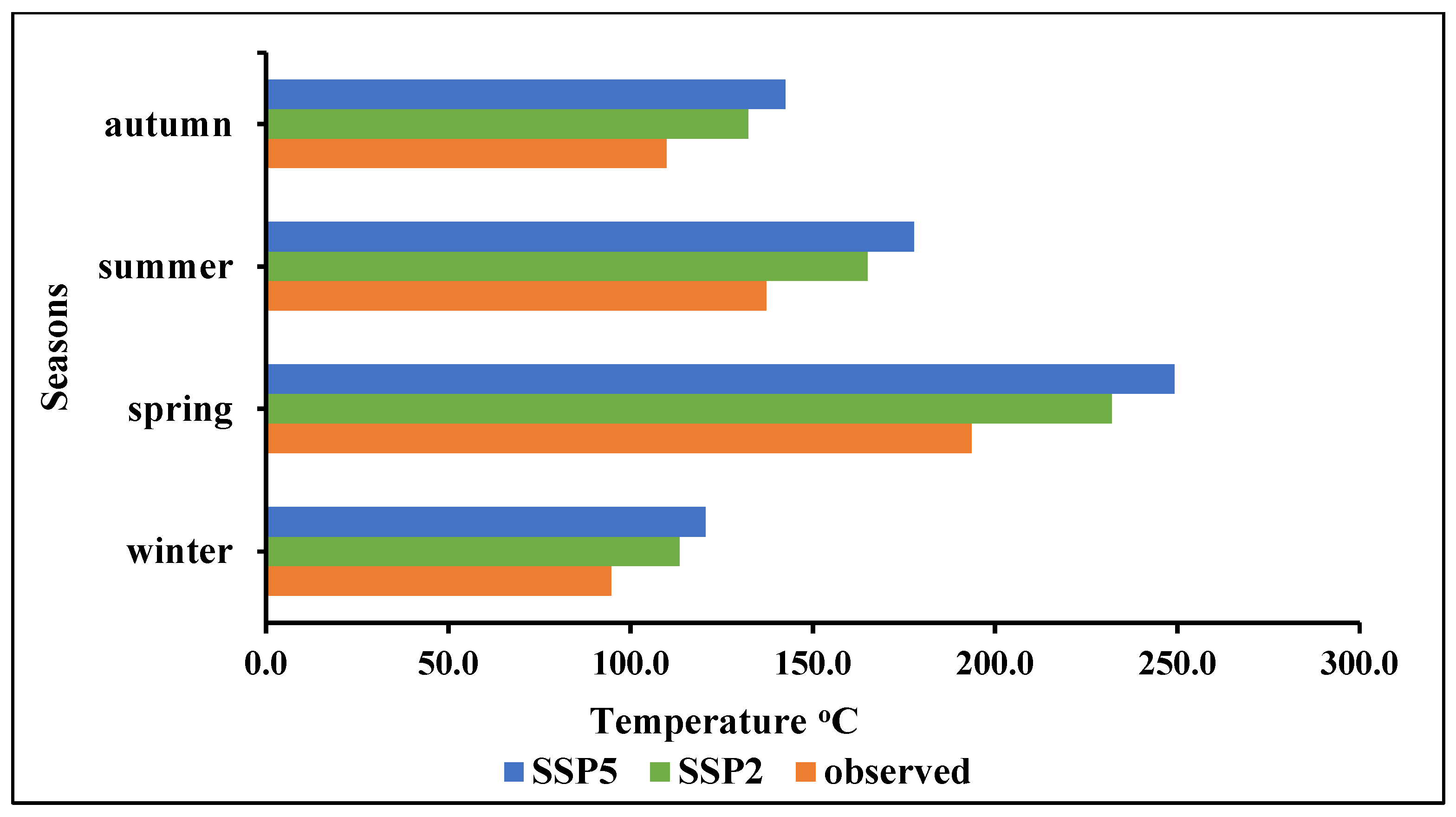
Winter, autumn, summer and spring and seasons are all included in the examination of precipitation change. The KRB’s seasonal variance precipitation is presented in
Figure 6. The amount of precipitation per month rises during each of four seasons. In the fall (winter), precipitation increases from 109.9 mm in baseline time frame to 142.5 mm (
Figure 6) according to the SSP5 scenario and to 132.3 mm (
Figure 6) according to the SSP2 scenario. This is the season with the biggest increase. The wintertime increase, on the other hand, is the smallest, with precipitation rising from 94.7 mm to 113.4 mm under SSP2 and to 120.6 mm (
Figure 6) under SSP5. The SSP2 and SSP5 scenarios, respectively, both depict an increase in precipitation across the spring and summer seasons. Spring precipitation increased from 193.6 mm to 232 mm and 249.3 mm, respectively, according to the SSP2 and SSP5 scenarios.
Figure 5 shows how summer precipitation increased at the end of the 21st century (2100), going from 137.3 mm to 165.1 mm and 177.7 mm.
3.8. Land Cover Change Trends
The Landsat images from 2000, 2010, and 2022 were combined and classified using the ArcGIS imagery classification tool. Nine land cover classes are represented by the resulting classified maps, which are displayed in
Figure 7. Landcover change trends for the century were shown in
Figure 8. These classes are Water, Forest, Vegetation, Flooded Vegetation, Crops, Shrub and Scrub, Built-up Area, Bare Ground, and Snow and Ice. The SWAT model was then fed these categorized maps as data. Future land cover conditions were taken into account when making land cover maps for the years 2040, 2070, and 2100 using TerrSet’s integrated Land Change Modeller. Prof. J. Ronald of Clark University created TerrSet in 1987, a thorough Geospatial Monitoring and Modelling System that makes use of the Cellular Automata-Markov Chain Model (CA-MCM) to project future changes in land cover.
Figure 7 illustrates the classified and projected land cover maps of study area. The results indicate a notable 21.4% increase in built-up area within the KRB from 2000 to 2100. On the other hand, the land cover classes of Water, Forest, Vegetation, Flooded Vegetation, Crops, Shrub and Scrub, Bare Ground, and Snow and Ice have experienced varying degrees of decline, with decreases of 4.4%, 2.8%, 2.4%, 1.8%, 1.6%, 0.1%, 1.7%, and 6.6%, respectively.
Table 10 provides a comprehensive overview of these changes in land cover classes.
3.9. SWAT Model Calibration and Validation
Optimizing a number of delicate factors linked to groundwater recharge, soil, snow and evapotranspiration is essential for calibrating the SWAT model.
Table 11 shows statistics for month’s hydrological model calibration and validation. This study found 17 variables that significantly affect the predicted outflow from the Kunhar River basin (
Table 12). These modelling variables were chosen in consideration of their significant contributions to evapotranspiration, runoff from snow melt, and recharge from groundwater, as well as the research on application of the SWAT model in glaciated watersheds [
43,
55,
56]. In the basin’s northern regions, a considerable portion of precipitation falls as snow during winter. Based on 30 years of river flow data from 1985 to 2014, the Kunhar River has an average annual discharge of 111.4 cubic meters per second (cumecs) as recorded at the Ghari Habibullah gauge. For the years 2001 to 2007, the model was calibrated (
Figure 9), primarily utilizing the monthly flow data gathered at the Ghari Habibullah gauge station. The model was then validated (
Figure 10) using data collected from observations between 2008 and 2014. It has been noted that the highest reported discharge occurs in month of July. R
2 and NSE values were employed to assess calibration and validation periods, as represented in
Table 11.
3.10. Effects of Climate on Stream Flows
After hydrological model was successfully calibrated and confirmed, the generated hydrological model was then utilized to project future streamflow patterns on a yearly timeframe for the period from 2015 to 2100. Two scenarios with various forecasted conditions each had their future flows evaluated.
Scenario-A: Taking into account the expected effects of CC, the first scenario’s forecast of flows was centered on an amalgam of the condition of the land cover currently and the predicted future climate.
Scenario-B: In this scenario, future land cover conditions and projected climatic conditions were utilized to examine the influence of future LULC and CC. This method made it possible to evaluate all potential consequences brought on by changes in both land cover and climate.
3.11. Scenario-A: Only Climate Change
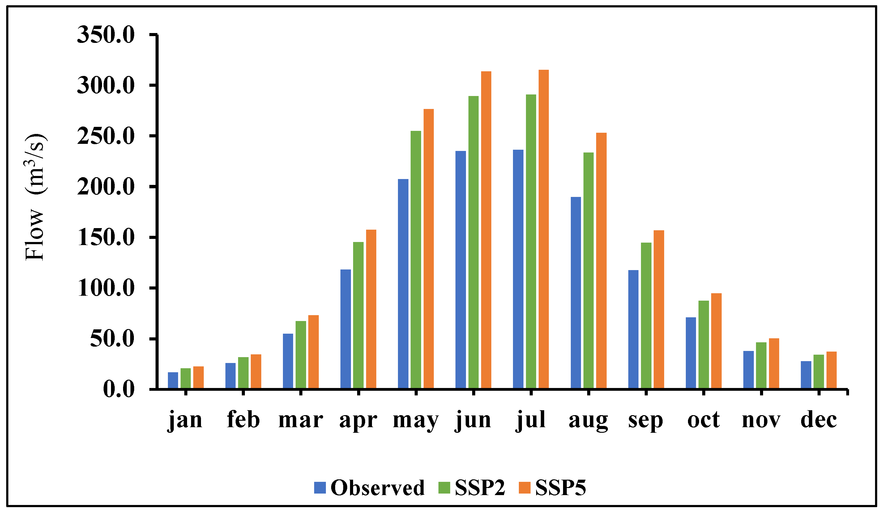
Using the calibrated model, flow predictions were made for the next three decades, taking into account climate change. The results indicated a 20.5% increase in precipitation under the SSP2 scenario and a 29.1% increase under the SSP5 scenario. Moreover, the maximum temperature showed a rise of 14.3% under SSP2 and 20.5% under SSP5, while the minimum temperature exhibited an increase ranging from 20.9% to 30.8% under SSP2 and SSP5 scenarios, respectively. The anticipated flows increased when the variations in temperature and precipitation were included in the calibrated SWAT model under assumption that land cover remained constant. The flows were specifically forecast to increase from 111.4 cumecs during base period (1999–2014) to 131.5 cumecs (a rise of 18.1%) under the SSP2 scenario and to 138.2 cumecs (an increase of 24%) under the SSP5 scenario in the future time frame (2015–2100).
Figure 11 compares monthly average flows for the base period (1999–2014) and future time period with respect to the SSP2 and SSP5 scenarios. KRB’s mean monthly flows will be examined for temporal fluctuations. Overall, both SSP scenarios suggest a tendency for flow to increase during the months that are historically characterized by low flow and high flow months. The mean seasonal flow is forecast to increase throughout the entire year, according to SSP2 and SSP5 scenarios. Notably, peak flows at dam site appear to have increased under both scenarios, which may be due to the influence of the westerlies circulation pattern. The higher flows during the winter season are probably a result of the increase in winter precipitation. It is important to note that both SSP scenarios predict July and January to have the highest and lowest flows, respectively.
3.12. Scenario-B: Climate and Land Cover Change
After the flows were anticipated based on CC, the calibrated hydrological model was utilized to project flows accounting for both land cover and climate change.
According to an estimate of land cover patterns, between 2000 and 2100, the populated area of KRB significantly increased by 21.4%. Conversely, other land cover classes such as Water, Forest, Vegetation, Flooded Vegetation, Crops, Shrub and Scrub, Bare Ground, and Snow and Ice showed varying degrees of decline, with magnitudes ranging from 0.1% to 6.6%. According to the SSP2 and SSP5 scenarios, precipitation increased to 20.5% and 29.1% as a result of climatic factors, respectively. Additionally, there was an upward trend in the maximum temperature, which increased by 14.3% and 20.5% according to the same conditions. SSP2 and SSP5 showed that the minimum temperature rose by 20.9% and 30.8%, respectively. The forecasts show an anticipated increase in flows when the future land cover conditions are incorporated into the calibrated SWAT model together with the changes in land cover and climate. The baseline era (1985–2014) recorded a flow of 111.4 cumecs, while the SSP2 and SSP5 scenarios project flows of 137 cumecs (a 23% increase) and 148.6 cumecs (a 33.4% increase) over the future time frame (2015–2100), respectively.
Figure 12 contrasts the average monthly flows for the base period (1999–2015) and future period according to the SSP2 and SSP5 scenarios. Analyzing the temporal variations in average monthly flows across the Kunhar River basin is the goal of this study. Both SSPs often show a rise in flow during both high and low flow months. Additionally, it is projected that the mean seasonal flow would continue to rise year-round. This rise in winter precipitation will likely result in higher winter flows. It is important to note that under both SSPs, July and January have the biggest and lowest flows, respectively.
4. Discussion
In the Hindukush Mountains, the Kunhar River watershed is located in a subtropical humid zone that is extremely susceptible to hydro-climatic changes [
52,
53]. Numerous CMIP6 GCMs have been used to evaluate effects of climate change on river flow patterns, offering important insights into probable future scenarios [
23,
57,
58,
59]. The objective of this study is to assess the impact of projected land cover and climate change on flow patterns of KRB, situated within UIB region. This was accomplished by using the output from the most trustworthy GCM out of four distinct models to calibrate a hydrological model. The calibrated model was then utilized to evaluate temporal implications of anticipated changes in land cover and climate on the basin’s hydrological characteristics. Based on the chosen GCM (MPI-ESM1-2-HR), the downscaled precipitation and temperature forecasts for the base period (1985–2014) demonstrated a satisfactory match with the gauge-based readings. This alignment could be attributed to the improved capability of CMIP6 models in accurately projecting temperature and precipitation patterns in HKH Region, as highlighted in previous studies [
43,
46].
Throughout the 21st century, the catchment region of KRB showed a consistent trend of long-term warming at both the annual and seasonal scales, according to the study of GCM outputs (MPI-ESM1-2-HR) [
60]. These findings align with previous studies conducted in neighboring regions of the Tibetan Plateau [
61,
62] and Himalayas [
48,
63,
64] indicating a widespread trend of increasing temperatures in South Asian regions. The increasing concentrations of greenhouse gases and aerosols in area can be blamed, at least in part, for the higher temperatures reported in the HKH Mountains [
52,
53,
65]. According to research by Bollasina et al. [
66] and Gohar et al. [
67], there is a rise in the concentration of atmospheric aerosols throughout Asia, which has been linked to significant temperature spikes in China. Furthermore, future projections suggest an expected increase in annual precipitation from 2015 to 2100, with evidence of increased flow in headwaters of the Yellow River basin during the same period [
68]. Precipitation is forecast to rise across the board throughout the upcoming year, while the summer and fall seasons are expected to experience the largest increases. These findings diverge from research performed in Malaysia’s Kelantan River basin and upper Cruz River basin, which found various precipitation patterns [
57,
69]. Furthermore, Ozturk et al. [
58] discovered a counterintuitive pattern of summer precipitation declines in westerly influenced areas such as Iran and Afghanistan. The seasonal Pr patterns, however, are in agreement with those observed in the Karakoram and Himalayan Mountain ranges and were found in the research areas. According to Babur et al. [
23], there is a persistent upward trend in seasonal and annual Pr for Jhelum River watershed, which is situated in Himalayan Range. Similar predictions were made by Garee et al. [
44] for Hunza River basin, which is close to Karakoram Range, about an increase in seasonal and annual precipitation. The consistency in results could be attributed to the Hindukush Range’s main westerlies circulation pattern [
65,
70,
71]. The rising level of anthropogenic absorbent aerosols in southern Asian atmosphere provides another explanation for the observed parallelism in precipitation patterns [
58,
66,
72].
According to the SWAT model research, SSP2 and SSP5 scenarios will both cause the annual average flow to rise in the future [
73,
74]. The anticipated increase in annual precipitation along with higher temperatures are to blame for this increase in flow. Immerzeel et al. [
73] have also predicted an increase in Indus River flow. Additionally, the anticipated research suggests that peak flows may change, moving from July to June by one month. This trend is result of a significant increase in precipitation right through springtime and wintertime months. A delay in Jhelum River’s peak flow, that normally happens between July and August, was noted by Babur et al. [
23]. The opposing expected patterns in summer and winter precipitation in the Hindukush and Himalayan Mountains may be to blame for this mismatch in findings.
This study holds significant practical implications; firstly, the findings can inform sustainable water resource management practices, aiding local authorities and policy makers in developing strategies to mitigate potential water scarcity issues [
75,
76,
77,
78,
79,
80,
81,
82]. Moreover, the results can guide the establishment of adaptive measures to safeguard water availability for agriculture, drinking water supply, and industrial use, particularly in the face of changing climate patterns [
83,
84,
85,
86,
87,
88,
89,
90,
91,
92]. Furthermore, this research can serve as a valuable resource for local communities, enabling them to make informed decisions about water usage and conservation. Additionally, this study contributes to the broader scientific understanding of how climate change interacts with land use dynamics to impact water resources, offering insights applicable to other regions facing similar challenges. Ultimately, the research not only addresses a critical gap in the literature but also equips stakeholders with the knowledge needed to navigate the complex and evolving landscape of water resource management in the Kunhar River basin and beyond.
5. Theoretical and Practical Implications
Firstly, the research advances our theoretical understanding of climate change dynamics in mountainous river basins. By revealing that both maximum and minimum temperatures are increasing alongside rising precipitation, it contributes to the body of knowledge on regional climate change patterns. This information can enrich climate models and theories, helping scientists and researchers better comprehend the complexities of climate change in such geographies. Secondly, this study delves into the intricate hydrological processes at play in mountainous river basins. It highlights the interplay between temperature, precipitation, and river flow, adding depth to our theoretical framework for comprehending how climate impacts water resources within these regions. This enhanced understanding is invaluable for predicting future changes and designing effective mitigation and adaptation strategies [
93,
94,
95,
96,
97,
98].
On the practical front, this study’s findings have several crucial implications. Firstly, the indication of increased flows underscores the importance of proactive water resource management. It suggests the need for adaptive measures to harness and manage the additional water resources effectively. This might involve optimizing reservoir management, implementing flood control measures, and ensuring sustainable water allocation practices. Secondly, the research contributes to building climate resilience in the region. Understanding the impacts of climate change is pivotal for crafting robust adaptation plans. This study’s insights can inform the development of climate-resilient infrastructure, such as improved flood defenses and water storage facilities, which are essential for coping with changing temperature and precipitation patterns. Thirdly, this study emphasizes the significance of responsible urban planning amidst increasing urbanization. As urban areas expand, their impact on river flows becomes more pronounced. Practical solutions, such as green infrastructure and sustainable land development practices, can help mitigate these impacts and ensure the sustainable growth of urban centers. Lastly, the research findings hold relevance for policymaking at various levels. They provide a foundation for evidence-based policies aimed at climate change mitigation and adaptation. Policy makers can use this information to draft regulations for reducing greenhouse gas emissions and formulate land use policies that minimize adverse effects on water resources.
In summary, this study’s theoretical implications advance our knowledge of climate change dynamics and hydrological processes, while its practical implications offer valuable guidance for water resource management, climate resilience building, urban planning, and policymaking in the Kunhar River basin and similar regions grappling with analogous challenges.
6. Conclusions
The goal of this study was to evaluate how the Kunhar River basin’s flows were affected by changing climatic conditions and land use. Two scenarios were considered: one focusing solely on climate change and the other incorporating both climate and land cover change. The investigation used two alternative shared socioeconomic pathways (SSP2 and SSP5) as baseline frameworks and covered the years 2015 to 2100. To project climate change, data from four GCMs were compared, with selection of the best-performing model. The following conclusions have been drawn from an examination of streamflow’s at Ghari Habibullah in the Kunhar River watershed under simulated future climate and land cover conditions:
- ⮚
The Kunhar River basin’s future time horizon (2015–2100) shows persistent rises in annual Tmax, Tmin and average temperature (Tavg) as well as Pr when compared to baseline period of 1985–2014. The rise in precipitation is expected to result in higher stream flows in future.
- ⮚
The mean daily flow at Kunhar River basin has increased under the current land cover conditions, rising from 111.4 cumecs between 1985 and 2014 to 131.5 cumecs according to SSP2 and 138.2 cumecs under SSP5.
- ⮚
According to the future land cover change scenario, the Kunhar River basin site’s flow is projected to increase from 111.4 cumecs (1999–2015) to 137 cumecs and 148.6 cumecs under SSP5.
- ⮚
The results show that the mean monthly flows are anticipated to rise under both SSPs by a range of 18–33.4% under the land cover and climate change scenarios.
- ⮚
The observed climate changes have translated into notable hydrological impacts, notably an increase in river flows. This change in flow patterns affects the timing and availability of water resources within the basin, with potential consequences for agriculture, ecosystems, and water supply.
- ⮚
This study has underscored the growing influence of urbanization on the basin’s hydrology. The expansion of urban areas has led to altered land use patterns, resulting in increased impervious surfaces and modifications to runoff processes. These changes add complexity to the basin’s hydrological dynamics.
The major goal of this study was to investigate anticipated fluctuations in Tmax, Tmin, and Pr and their possible effect on stream flows in the KRB. Certainly, this study’s integration of GCM simulations, statistical downscaling with CMhyd, and hydrological modeling with the SWAT represents a valuable approach to understanding the impacts of climate change and land use changes on water resources. However, it’s important to acknowledge several key limitations that can guide future research endeavors. Firstly, this study’s reliance on GCMs introduces inherent uncertainties associated with climate projections. These models provide a broad-scale view of future climate patterns, but their resolution may not capture regional variations adequately. Future research can explore ensemble modeling techniques to better quantify uncertainty and provide a range of possible outcomes.
Secondly, while statistical downscaling techniques such as CMhyd help bridge the gap between global climate models and local hydrological impacts, they are not immune to error. Further refinement and validation of downscaling methods, especially in regions with complex terrain or sparse observational data, are essential for improving accuracy. Additionally, addressing the limitations of input data quality, such as land cover maps and terrain information, should be a priority to enhance the reliability of model outputs. In terms of potential future developments, researchers can explore advanced model integration approaches that combine multiple GCMs, downscaling techniques, and hydrological models to reduce uncertainties. This ensemble modeling can provide a more comprehensive understanding of potential future scenarios and their associated risks.
Furthermore, future studies can delve into scenario analysis by considering a broader range of socioeconomic and policy scenarios. These scenarios can encompass various land use and climate change mitigation strategies, helping decision-makers plan for multiple futures. Additionally, involving local stakeholders and communities in the research process can offer valuable insights and ensure that study findings are tailored to address regional challenges effectively. By adopting a holistic approach that includes improved data quality, advanced modeling techniques, and scenario analysis, future research can provide more robust and actionable insights for sustainable water resource management in the face of climate and land use changes. The findings of this study are essential for formulating regional development strategies, implementing adaptation plans, and organizing and administering water management projects such as irrigation and hydropower in a sustainable manner.


 ,
, 


