Article

An Alternative Method for Estimating the Peak Flow for a Regional Catchment Considering the Uncertainty via Continuous Simulation

1
School of Engineering, University of Southern Queensland, Toowoomba 4350, Australia
2
Murray-Darling Basin Authority, Australian Capital Territory, Canberra City 2601, Australia
*
Author to whom correspondence should be addressed.
Water 2023, 15(19), 3355; https://doi.org/10.3390/w15193355
Submission received: 14 August 2023 / Revised: 13 September 2023 / Accepted: 20 September 2023 / Published: 25 September 2023

Abstract

:
Estimating peak flow for a catchment is commonly undertaken using the design event method; however, this method does not allow for the understanding of uncertainty in the result. This research first presents a simplified method of fragments approach to rainfall disaggregation that ignores the need to consider seasonality, offering a greater diversity in storm patterns within the resulting sub-daily rainfall. By simulating 20 iterations of the disaggregated sub-daily rainfall within a calibrated continuous simulation hydrologic model, we were able to produce multiple long series of streamflow at the outlet of the catchment. With these data, we investigated the use of both the annual maximum and peaks over threshold approaches to flood frequency analysis and found that for a 1-in-100-year annual exceedance probability peak flow, the peaks over threshold method (333 m3/s ± 50 m3/s) was significantly less uncertain than the annual maximum method (427 m3/s ± 100 m3/s). For the 1-in-100-year annual exceedance probability, the median peak flow from the peaks over threshold method (333 m3/s) produced an outcome comparable to the design event method peak flow (328 m3/s), indicating that this research offers an alternative approach to estimating peak flow, with the additional benefit of understanding the uncertainty in the estimation. Finally, this paper highlighted the impact that length and period of streamflow has on peak flow estimation and noted that previous assumptions around the minimum length of gauged streamflow required for flood frequency analysis may not be appropriate in particular catchments.

1. Introduction

Estimating peak flow rates from a catchment has long been a focus of engineering hydrologists and is fundamental to the design of flood protection infrastructure [1,2,3,4]. Understanding the uncertainty associated with peak flow estimation is, however, often neglected by practitioners, despite the acceptance that many sources of uncertainty exist [1,5,6,7]. The commonly used design event method requires antecedent moisture conditions to be adjusted to ensure a probability-neutral conversion of rainfall to runoff [4,8,9,10]. Ref. [11] detailed the benefits of continuous simulation over the design event method with their development of a calibrated hydrologic model in a regional town in the state of Queensland, Australia. This paper expands on the research undertaken by the authors [11], whose focus was the calibration of the continuous simulation hydrologic model to historical events, with the aim of deriving flood frequency estimates with a greater understanding of uncertainty.
To estimate peak flows from a continuous simulation model, the data should normally follow a flood frequency distribution similar to gauged streamflow records. A model that can replicate a long series of streamflow (i.e., continuous simulation) can assist in overcoming the shortcomings of stream gauge data, most noticeably the impact of urbanisation [1]. A flood frequency analysis (FFA) can be undertaken using one of two sampling approaches: annual maximum series and peaks over threshold (also known as partial series) [12]. The annual maximum series, while easier to identify independent flood events, produces fewer data points than the peaks over threshold series [13] but also prioritises the maximum annual flood over multiple larger floods that may have occurred in the same year. In contrast, the peaks over threshold approach offers added complexity due to the requirement of selecting an appropriate threshold flow. Some researchers found the best results of their FFA occurred when the number of data points (m) equalled the years of data (n) [11,14,15], while others recommended a ratio of 1 m:3 n [16]. Both sampling approaches rely on a long series of continuous streamflow, with at least 50 years of data recommended to be used [17].
To produce a long series of continuous streamflow, a continuous simulation model requires an extended period of recorded rainfall at a suitable time step for the size and level of urbanisation of the catchment [18]. In the case of a relatively small urban catchment, rainfall at a sub-hourly interval is required. Obtaining a recorded rainfall series of sufficient length over this time scale is extremely challenging given the lack of sub-daily rainfall gauges available not only globally [19] but more relevant to this research in sparsely populated countries such as Australia [20]. This contrasts recent reviews of global precipitation data, with some locations offering sub-daily rainfall that spans multiple decades [21]. The availability of sub-daily rainfall data has supported recent advancements in the use of continuous simulation hydrologic modelling [22]; however, this research is unique in that the lack of availability of site-based sub-daily rainfall data requires alternate considerations. To address this issue, sub-daily rainfall can be generated from coarser timescale (daily) rainfall records via disaggregation [23] if historical daily rainfall data for at least 100 years are available for the site [24].
The most commonly used rainfall disaggregation approaches are summarised in the literature [23], including parametric sampling methods such as the Poisson-cluster models and the random scale models, as well as nonparametric sampling methods such as the Method of Fragments (MoF). They concluded that the MoF, first proposed as a method to disaggregate streamflow [25], was more flexible for operational use. At its core, the MoF simply disaggregates daily rainfall by selecting the pattern or ‘fragments’ of a known sub-daily event. The process of selection of suitable sub-daily events varies across the literature, including the use of the previous and subsequent day wetness to limit the sample size [26] or adding classes based on rainfall magnitude to ensure the daily rainfall was disaggregated based on sub-daily rainfall of a similar magnitude, as well as limiting the selection to events that occurred in the same month as the disaggregated rainfall [23]. While a long series of sub-daily rainfall data was produced, neither study used their dataset for continuous hydrologic modelling to estimate flood frequency.
This research offers new insight via the presentation of an alternate method for estimating peak flow in a small regional urban catchment. Via the inclusion of associated uncertainty, this method also offers practical insight into how accurate regional authorities should consider their hydrological assessments to be. The results of this research also contribute significantly to the understanding of hydrologic uncertainty, especially in an urban catchment where the reliance on accurate hydrologic modelling is at its’ greatest. By assessing the impact that the length and period of streamflow series has on peak flow estimation, we highlight the limitations associated with peak flow estimations from gauged catchments.
In particular, this research aims to develop a long series of sub-daily (6 min) rainfall data for use in a continuous simulation model using a simplified version of the MoF and a long series of continuous flow data using the calibrated hydrologic model developed by the authors [11]. It will also estimate, with uncertainty, the peak flow for a range of annual exceedance probabilities and compare the results of this research to other methods. The materials and methods used in this research are described in Section 2, while Section 3 presents and discusses the results. Finally, our conclusions are presented in Section 4.

2. Materials and Methods

2.1. Continuous Simulation Model

A continuous simulation model was used in this research to estimate the peak flow for different annual exceedance probabilities. The model was developed by the authors [11] for the Gowrie Creek catchment, a heavily urbanised 50 km2 catchment in the regional city of Toowoomba, in the state of Queensland, Australia. Toowoomba is considered to be sub-tropical with an average annual rainfall of 700 mm, the majority of which falls over the wet season from November to March. The extent of the catchment and its location in Australia are shown in Figure 1. The following two paragraphs summarise the hydrologic model and the key calibrated loss parameters.
An XPRAFTS semi-distributed hydrological model was used to represent the Gowrie Creek system. The overall catchment was delineated into 23 sub-catchments, with each sub-catchment having a unique impervious fraction determined via regression analysis. The previous area loss within this software is represented by the ARBM dynamic loss approach [27,28]. This loss approach can be visualised as a series of interconnected buckets of varying sizes. Rainfall that is not intercepted by trees or plants (Interception Storage Capacity (ISC)) may be captured in minor surface depressions (Depression Storage Capacity (DSC)). If the rainfall is intense enough, runoff may result from the DSC, otherwise infiltration to the Upper Soil Capacity (USC) occurs. Water is redistributed between the USC and the Lower Storage Capacity (LSC) depending on the capacity available within the bucket. Water from the LSC can then be drained into the Groundwater Storage Capacity (GSC), which contributes to baseflow. The ARBM allows for the simulation of soil moisture depletion via evaporation between rainfall events [29] with evapotranspiration depleting the ISC, DSC, USC, and LSC. Any excess rainfall is routed to the catchment outlet based on the non-linear runoff-routing method [30]. The model was calibrated using the two-stage calibration approach [31,32]. The model offered a satisfactory fit (Nash Sutcliffe Efficiency > 0.5) for 9 of the 11 selected storm events, with seven events exceeding a Nash Sutcliffe Efficiency of 0.75. Events used in the calibration/validation included peak flows as low as 9 m3/s and as high as 600 m3/s. The calibrated ARBM parameters are shown in Table 1.
A challenge identified in the calibration approach was the lag present when comparing the model simulations to the available streamflow data. This issue is not uncommon [33] and was noted to be likely due to the simplified way the hydrologic model responds to rainfall and can vary with changing rainfall intensity [34,35,36]. Despite this issue, the strong calibration achieved suggests the model adequately represents the magnitude of the runoff, which is the focus of this research.
While models for the catchment were calibrated to the historic rainfall and streamflow records, this research required additional steps to enable the continuous simulation model to be developed. Initially, daily rainfall data within the catchment for a 100-year period were obtained to allow the sub-daily rainfall disaggregation to be undertaken. This 100-year series of sub-daily rainfall data could then be simulated in a continuous simulation model to produce a 100-year time series of simulated streamflow. An FFA of this simulated streamflow was then undertaken to estimate peak flows of varying flood frequencies. This approach was repeated for 20 sub-daily rainfall disaggregation scenarios to facilitate the estimation of uncertainty in the results.

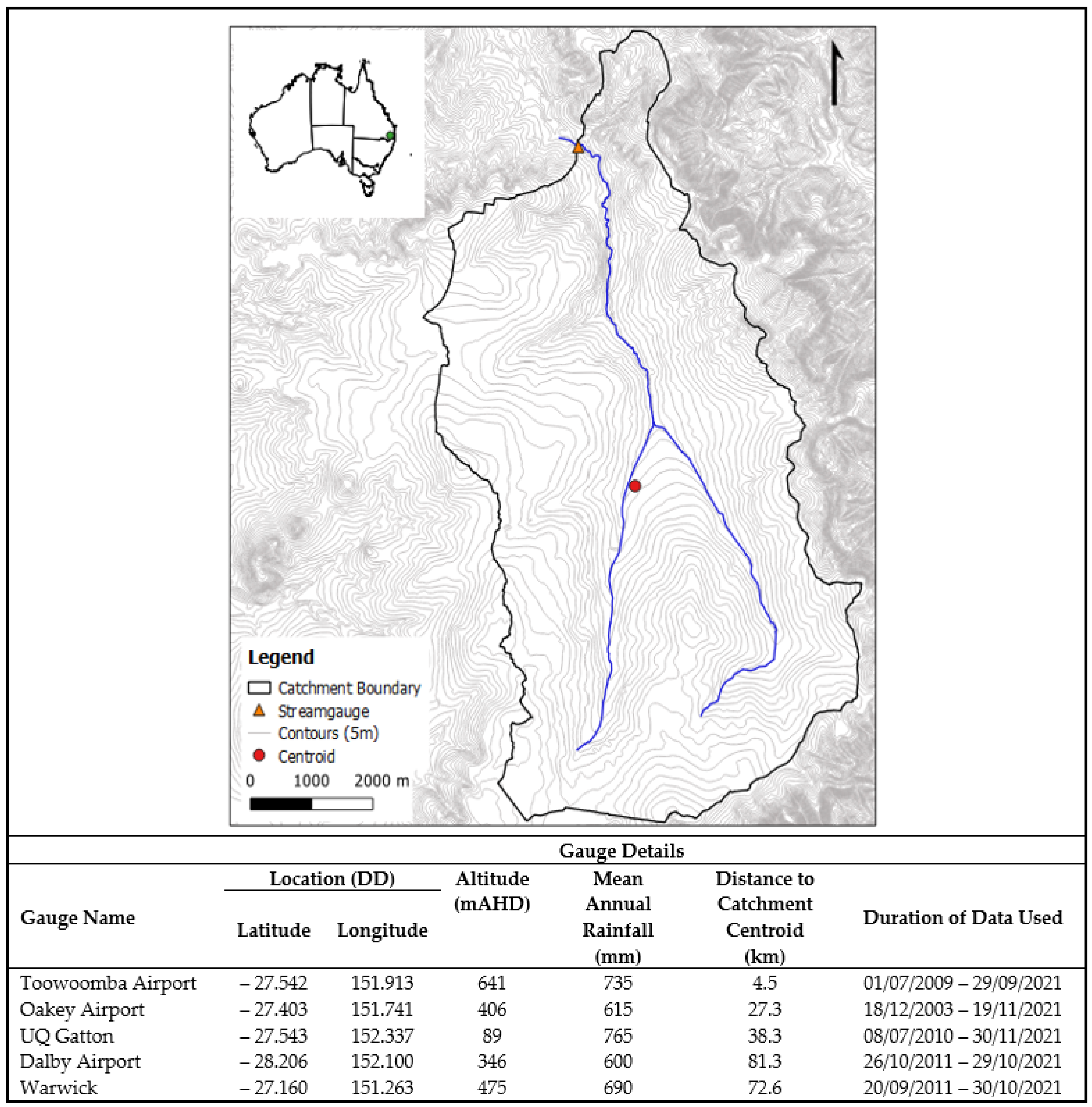
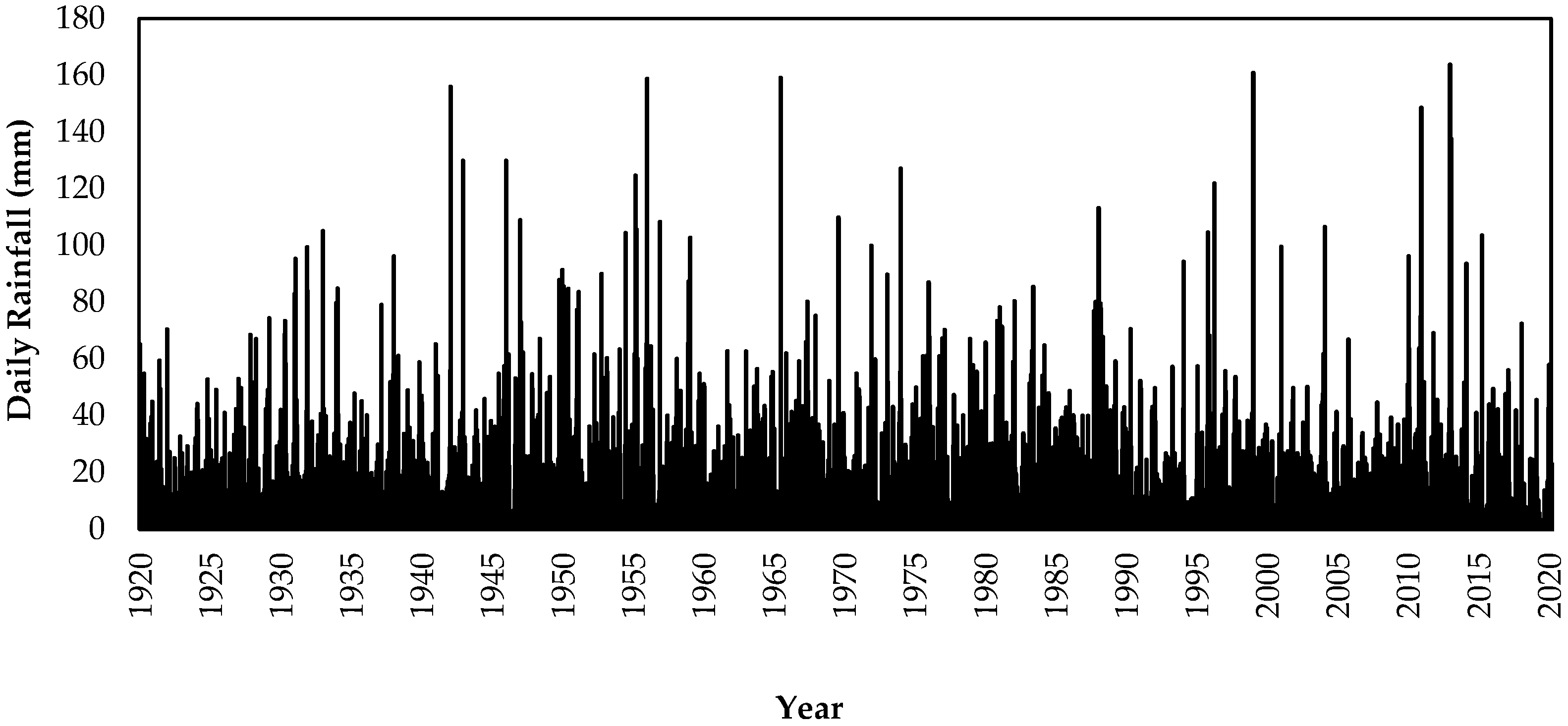
2.2. Daily Rainfall Data

Historical daily rainfall at the centroid of the catchment was sourced from SILO, a Queensland Government database containing continuous daily climate data for Australia from 1889 to the present day [24]. The 100 years of daily rainfall (year 1920 to 2020) used in this research are shown in Figure 2.

2.3. Sub-Daily Rainfall Data

A long, continuous series of historical sub-daily rainfall data with a timestep shorter than the intended disaggregated timestep is needed to disaggregate the daily rainfall using the MoF. Historical sub-daily rainfall data are, however, limited in Australia [20]. To extend the sub-daily rainfall data duration and allow a wider variety of storm temporal patterns to be used, shorter durations of data from multiple gauging stations surrounding the catchment were sourced and ‘stacked’ to create a single longer series. This approach was used by [23] and found to achieve similar results to adopting a single sub-daily rainfall dataset. For the Gowrie Creek catchment specifically, only 12 years of sub-daily rainfall data were available; therefore, data from rain gauges located outside the catchment were sourced. The location of the catchment and proximity and duration of the historical sub-daily rainfall were sourced from the Bureau of Meteorology and used in the rainfall disaggregation, as shown previously in Figure 1.

2.4. Daily Rainfall Disaggregation

2.4.1. Method of Fragments

The MoF approach used six major steps to disaggregate historical daily rainfall based on sub-daily rainfall data from multiple representative rainfall stations [23]. A key difference in this research was the exclusion of the need to only disaggregate daily rainfall using sub-daily storms that occur at a similar time of year or have similar rainfall on the day before or after the target day. The reasons for this are discussed further in Section 2.4.4.
The key steps adopted in this research to disaggregate historic daily rainfall from sub-daily rainfall were
  • Assign a storm class to both the historic daily and sub-daily rainfall series;
  • Assign a unique storm number to each historic sub-daily storm;
  • For a given day ‘x’ in the daily rainfall series, select a sub-daily storm with the same Storm Class;
  • Disaggregate the daily rainfall based on the pattern of the sub-daily storm.
  • Repeat Steps 3 and 4, ensuring the sub-daily storms are chosen uniformly to create an ensemble of disaggregated rainfall;
  • Repeat all steps multiple times to create multiple iterations of disaggregated rainfall to understand the uncertainty.

2.4.2. Storm Class

An important consideration when using the MoF is the storm class. The storm class defines how the daily and sub-daily rainfall data sets are related as the daily rainfall data are only disaggregated to storms within the same storm class. It was initially suggested that only four storm classes be selected based on the rainfall before and after the day of interest [26]. However, this has a number of limitations including the potential for not considering important storms based on their insignificant pre/post-day rainfall total. In addition, large daily rainfall totals could be disaggregated into high-intensity, short-duration, and low-depth storms based on the same pre/post-rainfall conditions, rather than basing them on the magnitude of rainfall on the day of interest. The latter issue is of particular interest if the disaggregated rainfall is to be used in a hydrological model.
As a result, dividing the rainfall data into a number of storm classes was subsequently suggested, with an interval of 5 mm being adopted [23]. This method was initially utilised in this research; however, there were too few storms available for less frequent/more extreme daily rainfall totals. It was evident that multiple storm class options had to be considered and evaluated to determine the best approach.

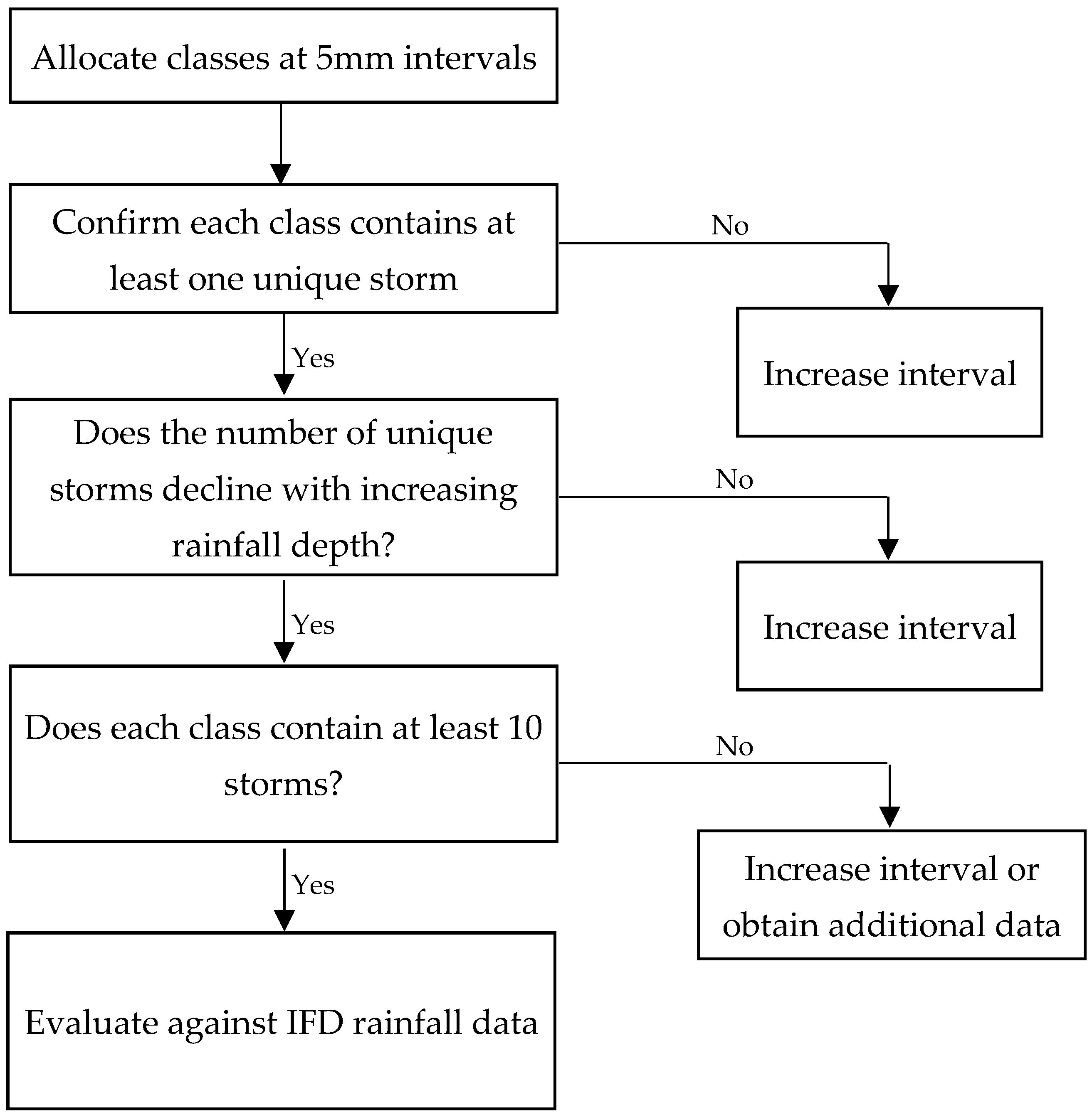
2.4.3. Determination of the Number of Storm Classes

To ensure that the MoF produced sub-daily rainfall data suitable for the hydrologic assessment, the results from three storm class options, presented in Table 2, were validated against the intensity-frequency-duration (IFD) data for the catchment. The IFD data represent design storm rainfall depths developed by the Australian Bureau of Meteorology and are commonly used in design event modelling. These storm class options were evaluated to validate the iterative approach presented in Figure 3, which was used in an attempt to optimise the number of storm classes within each option.
To directly evaluate the MoF results from the class options assessed, IFD data were developed from the generated sub-daily rainfall. The annual maximum series was first modelled to the Generalised Extreme Value (GEV) distribution, as per the Bureau of Meteorology methodology for generating IFD data from historical sub-daily rainfall data [37]. A direct comparison of the MoF-generated design rainfall depths to the Bureau of Meteorology-generated design rainfall depths for the same duration and annual exceedance probability for different storm class options is shown in Figure 4. From this comparison, it was clear that class option 2 produced the best fit due to its proximity to the 1 in 1 line and was subsequently used in this research. The results suggest when moderate (>25 mm/day) to extreme (>75 mm/day) rainfall depths are reached, the size of the class should be increased to allow a greater range of storms to be selected. Providing a larger number of smaller classes (class option 1) resulted in fewer storms to choose from, thereby decreasing the representation of moderate to extreme rainfall events, while a smaller number of larger classes (class option 3) resulted in moderate daily rainfall depths being associated with more extreme storm patterns.
As the disaggregated sub-daily rainfall covered the same time period as the recorded sub-daily rainfall, it was possible to directly compare the maximum rainfall from critical storm durations for the size of the catchment, namely those from 30 min to 360 min, for each year. While the MoF is not intended to replicate recorded sub-daily rainfall nor be used for hindcasting [38,39,40] and in turn unlikely to replicate recorded rainfall, comparing the disaggregated rainfall to the nearby Toowoomba Airport gauge for these critical storm durations (refer to Figure 5) showed that it was able to maintain key statistics, including the median and mean. This result provided additional support for the use of the MoF and the adoption of class option 2.

2.4.4. Seasonality

To best represent the range of storms possible and to understand the impact various storm patterns have on the catchment response to rainfall, it is important that a larger quantity of storms is available for use in the disaggregation. When reviewing the sub-daily rainfall data used in this research, it was clear that as the rainfall amount increased, the number of storms decreased significantly, as shown in Figure 6. Previous studies that used the MoF approach ([8,20,23]) constrained the storm selection by incorporating seasonality, whereby the range of storms available for disaggregation was limited to those within a preset window around the day of rainfall being disaggregated. These previous studies did not, however, use the disaggregated rainfall in a hydrology model nor did they compare the results to IFD data. If this was undertaken, they would likely have seen that the same storm patterns would have been chosen multiple times to disaggregate the more extreme daily rainfall totals, and therefore produced similar peak flows, volumes, and timing for multiple events, likely skewing any flood frequency analysis undertaken. To overcome this issue, this research excluded seasonality as a constraint on storm selection and instead adopted an approach whereby multiple iterations of disaggregated rainfall were simulated to better understand the uncertainty associated with storm selection.

2.5. Hydrologic Model Simulation

The calibrated continuous simulation hydrologic model developed by the authors [11] was used in this research. The hydrologic model was simulated for a period of 100 years (1920 to 2020) of disaggregated historical daily rainfall. Twenty iterations of the disaggregated rainfall were simulated to allow the uncertainty in the results to be determined. While the model run times made running additional iterations prohibitive, increasing the number of iterations would have minimal impact on the outcomes of the research due to the small number of unique iterations possible, in particular for larger daily rainfall totals (as presented in Figure 6). This issue is further explored in Section 3.3.

2.6. Determination of Threshold Value

To allow the peaks over threshold flood frequency analysis of the long series of flow rates determined via continuous simulation, a threshold value is required. The data series used to undertake the flood frequency analysis is the maximum monthly flows above the threshold value. A higher threshold value will result in fewer values in the data series, while a lower threshold value will result in the opposite. In this research, we proposed an alternate method where we graphically interrogated the peak monthly flow from the full 100 years of continuous flow ranked in ascending order to determine clear changes in trend. Figure 7 shows three clear changes in trend at 45 m3/s, 70 m3/s and 110 m3/s.
Adopting the higher value of 110 m3/s resulted in a 0.5m:1n ratio, which was considered a data series too small for a flood frequency analysis [14]. Adopting the lower value of 45 m3/s resulted in a 3.2 m:1 n ratio, significantly higher than those documented in the literature [14,15]. In addition, the trend change noted at 45 m3/s was not as clear as the other two changes in slope. Adopting the middle value of 70 m3/s resulted in a 1.2m:1n ratio, which is in line with those documented in the literature [14,15], and graphically represents a clear change in trend, suggesting the flows below 70 m3/s would have a very frequent recurrence interval.

3. Results

3.1. Flood Frequency Analysis

A flood frequency analysis of all 20 iterations of the continuous simulation model was undertaken on the peaks over threshold series using a Bayesian fit of the Log Pearson Type 3 (LPIII) distribution [1]. The same flood frequency analysis was also undertaken using the available stream gauge data with the combined results shown in Figure 8. As shown, all 20 simulations are within a relatively tight band. Given that all results are equally likely, we considered that the median would approximate the peak flow for a given Annual Exceedance Probability (AEP), with the range of possible results (or uncertainty bounds) being within the highest and lowest results of the simulation. This suggests that the 1-in-10-year AEP peak flow would be 166 m3/s ± 20 m3/s, while the 1-in-100-year AEP peak flow would be 333 m3/s ± 50 m3/s.
In addition to the main finding above, the performance of the simulated results is also supported by the proximity of the same flood frequency analysis undertaken on the stream gauge. While the stream gauge result is at the upper end of the range of simulated results, it is posited that the shorter length of available stream gauge data (52 years), in comparison to the model simulations (100 years), potentially skews the stream gauge results. If the flood frequency analysis of the simulated results was undertaken for the same period and length of available stream gauge data (refer to Figure 9), the simulated results would better reflect the stream gauge data. What is also evident, however, is that the range of possible solutions increases significantly. Using the same approach as above, the 1-in-10-year AEP peak flow increases to 172 m3/s ± 30 m3/s, while the 1-in-100-year AEP peak flow would increase to 360 m3/s ± 100 m3/s. In practice, it is recommended that at least 50 years of data be used in a flood frequency analysis [17]. This research indicates that data of this length may, however, overestimate the result and increase the uncertainty significantly.
While the length of available data is a well-discussed criterion when undertaking a flood frequency analysis [17], the period of data adopted is often neglected. This issue is particularly evident in catchments such as the Gowrie Creek catchment, which may be considered to have a sufficient length of gauged data but recently experienced a flood event significantly larger than any others recorded. The impact of adopting the minimum of 50 years of streamflows over differing time periods (1920–1970, 1930–1980, 1940–1990, 1950–2000, 1960–2010, and 1970–2020) was undertaken using one of the model simulations and is shown in Figure 10. These results show the impact that large floods (or the lack thereof) can have on the flood frequency analysis, with the 1-in-100-year AEP peak flow ranging from 308 m3/s to 432 m3/s.

3.2. Peaks over Threshold vs. Annual Maximum Series

As detailed in Section 1, the peaks over threshold method was used in this research to develop the data series for flood frequency analysis. However, the annual maximum series is still used by most practitioners, and it was therefore worth highlighting the impact of adopting the alternative option. The results presented in Figure 11 show that the annual maximum series results in significantly higher peak flows for AEPs less frequent than 1 in 5 years while also resulting in increased uncertainty in the result. For example, the 1-in-100-year AEP using the peaks over threshold approach was estimated to be 333 m3/s ± 50 m3/s, while using the maximum series approach, it was 427 m3/s ± 100 m3/s.

3.3. Impact of the Number of Disaggregated Rainfall Iterations

While the software used in this research was limited due to the number of disaggregated rainfall iterations that could be simulated in a reasonable timeframe, the results shown in Figure 12 support the previous hypothesis that increasing the number of simulations beyond 20 would not have a significant impact. When viewing the change in the median peak flow for the 1-in-100-year AEP with each new iteration, it can be seen that there is a small variation in the result (between 320 m3/s and 340 m3/s), with an even tighter range (between 320 m3/s and 330 m3/s) forming beyond 11 iterations. This is likely due to the range of the results plateauing after the same number of iterations, suggesting that the upper and lower bounds of the 1-in-100-year AEP peak flow was reached based on the rainfall data used. Adding new sub-daily storms based on additional data collected over time would likely change this result. However, it is unlikely to be significant based on the narrow range of median peak flows.

3.4. Comparison to Other Methods

Two previous hydrological assessments of the Gowrie Creek catchment were undertaken in the wake of the significant flooding in 2011. In 2013, the design event method was used to estimate the peak flow at the stream gauge for a range of AEPs from the 1-in-2-year to the 1-in-100-year AEPs (AECOM, 2013). An alternative approach to estimating peak flow was proposed by [41] who applied a Monte Carlo framework to the simplistic rational method (naming it the Rational Monte Carlo (RMC) method) to estimate peak flows for the same range. The results of these assessments in addition to the outcomes of this research are presented in Figure 13.
From this comparison, it is evident that the results of this research show a strong correlation with the design event method for all AEPs, while also showing good agreement with the RMC method for the 1-in-2 year and 1-in-5-year AEPs. It is noticeable, however, that there is a significant divergence from the RMC when the AEP becomes less frequent. This is likely due to the differing treatment of hydrologic losses, with this research adopting a dynamic loss model discussed in [11], while the RMC method adopts a simplistic runoff coefficient.

3.5. Review of an Individual Flood Event

While determining the peak flow for a given annual exceedance probability was the key outcome of this research, it was also interesting to compare the results of all scenarios simulated against the recorded streamflow for a given historical event. The major flooding that occurred in the Gowrie Creek catchment in January 2011 was an obvious candidate for comparison. The results shown in Figure 14 highlight that different rainfall temporal patterns were chosen to represent the same total daily rainfall. While the inconsistencies of the stream gauge during this event were documented by the authors [11]. It is still worth noting that all peak flows were less than the ~600 m3/s recorded by the stream gauge, with a concentration of scenarios around a peak of 400 m3/s. This suggests that a similar rainfall temporal pattern was chosen multiple times during the disaggregation process, which is consistent with the limited availability of large storm patterns as shown previously in Figure 6, and further supports the insignificant impact additional iterations would have on the result.

4. Conclusions

This research investigated the use of a calibrated continuous simulation model using the industry standard hydrology model XPRafts to estimate peak flows for a range of annual exceedance probabilities with uncertainty.
The need for a continuous series of sub-daily rainfall data for use in a continuous simulation model highlighted the requirement for a rainfall disaggregation model to disaggregate a long series of historic daily rainfall to a sub-daily scale. The use of a modified MoF that excluded seasonality and pre/post rainfall conditions allowed for a significant increase in the number of storms to be selected within a given class and allowed for the uncertainty to be better understood. The results of this method showed a strong correlation to the Bureau of Meteorology IFD design rainfall, justifying the use of this alternative method over those previously documented in the literature. This is a significant outcome, as it provides an alternate methodology to produce disaggregated rainfall better suited for continuous simulation modelling.
To understand the uncertainty in the result, 20 simulations of the calibrated hydrologic model with different disaggregated rainfall series were undertaken. A flood frequency analysis using the peaks over threshold method allowed the estimation of peak flows for different annual exceedance probabilities. The relatively tight range of results suggested there was limited uncertainty in the result, which is an important understanding when undertaking hydrologic modelling in an urban catchment.
This research further investigated the use of different flood frequency analysis methods and the use of different quantities and periods of streamflow data. When the flood frequency analysis of the model simulations (100 years of streamflow) was compared to the stream gauge (52 years of streamflow), it was evident that the stream gauge result was higher than all modelled results. If the flood frequency analysis of the model simulations was reduced to the same number of years and time period, the stream gauge result was close to the median of the modelled results. It was also shown that if 50 years of data were selected from differing time periods, the results of a flood frequency analysis could vary significantly. This result is of significance to practitioners who rely on flood frequency analyses of poorly gauged catchments to make informed decisions.
This research compared the peaks over threshold and the annual maximum series methods and showed that the use of the annual maximum series results in significantly more uncertainty in comparison to the peaks over threshold approach. Understanding the uncertainty of each method will assist practitioners who may seek to utilise alternative methods in evaluating the peak discharge in a catchment.
Finally, we were able to compare our result to other methods previously adopted for this catchment and found good agreement with the design event method. This result suggests the new methods being adopted within this research are comparable to other methods whilst also providing an improved understanding of the uncertainty. This research can be extended to extract hydrographs to determine the impact hydrologic uncertainty has on hydraulic modelling.

Author Contributions

Conceptualization, I.B.; methodology and investigation, I.B.; software, I.B.; validation, K.M., S.C. and M.J.A.; writing—original draft preparation, I.B.; writing—review and editing, K.M., S.C. and M.J.A.; supervision, K.M., S.C. and M.J.A.; funding acquisition, K.M. All authors have read and agreed to the published version of the manuscript.

Funding

This research was funded by the Toowoomba Regional Council.

Data Availability Statement

Data used or generated as part of this research will not be made publicly available due to licensing agreements.

Acknowledgments

The authors thank the Toowoomba Regional Council for the data supplied to complete this research. Their contribution allowed this research to be completed in a way that may offer significant community and industry benefits.

Conflicts of Interest

The authors declare no conflict of interest.

References

  1. Ball, J.; Babister, M.; Nathan, R.; Weeks, W.; Weinmann, P.E.; Retallick, M.; Testoni, I. A Guide to Australian Rainfall and Runoff; Commonwealth of Australia (Geoscience Australia): Canberra, Australia, 2016; Available online: http://hdl.handle.net/11343/119609 (accessed on 19 July 2022).
  2. Kastridis, A.; Theodosiou, G.; Fotiadis, G. Investigation of flood management and mitigation measures in ungauged natura protected watersheds. Hydrology 2021, 8, 170. [Google Scholar] [CrossRef]
  3. Segura-Beltrán, F.; Sanchis-Ibor, C.; Morales-Hernández, M.; González-Sanchis, M.; Bussi, G.; Ortiz, E. Using post-flood surveys and geomorphologic mapping to evaluate hydrological and hydraulic models: The flash flood of the Girona River (Spain) in 2007. J. Hydrol. 2016, 541, 310–329. [Google Scholar] [CrossRef]
  4. Hossain, S.; Hewa, G.A.; Wella-Hewage, S. A comparison of continuous and event-based rainfall-runoff (RR) modelling using EPA-SWMM. Water 2019, 11, 611. [Google Scholar] [CrossRef]
  5. Moges, E.; Demissie, Y.; Larsen, L.; Yassin, F. Review: Sources of hydrological model uncertainties and advances in their analysis. Water 2021, 13, 28. [Google Scholar] [CrossRef]
  6. Kastridis, A.; Kirkenidis, C.; Sapountzis, M. An integrated approach of flash flood analysis in ungauged Mediterranean watersheds using post-flood surveys and unmanned aerial vehicles. Hydrol. Process. 2020, 34, 4920–4939. [Google Scholar] [CrossRef]
  7. Kaffas, K.; Hrissanthou, V. Application of a continuous Rainfall-Runoff model to the basin of Kosynthos river using the hydrologic software HEC-HMS. Glob. NEST J. 2014, 16, 188–203. [Google Scholar]
  8. Pathiraja, S.; Westra, S.; Sharma, A. Why continuous simulation? The role of antecedent moisture in design flood estimation. Water Resour. Res. 2012, 48, 1–15. [Google Scholar] [CrossRef]
  9. Cameron, D.S.; Beven, K.J.; Tawn, J.; Blazkova, S.; Naden, P. Flood frequency estimation by continuous simulation for a gauged upland catchment (with uncertainty). J. Hydrol. 1999, 219, 169–187. [Google Scholar] [CrossRef]
  10. Borga, M.; Anagnostou, E.N.; Blöschl, G.; Creutin, J.D. Flash floods: Observations and analysis of hydro-meteorological controls. J. Hydrol. 2010, 394, 1–3. [Google Scholar] [CrossRef]
  11. Brown, I.W.; McDougall, K.; Alam, M.J.; Chowdhury, R.; Chadalavada, S. Calibration of a continuous hydrologic simulation model in the urban Gowrie Creek catchment in Toowoomba, Australia. J. Hydrol. Reg. Stud. 2022, 40, 101021. [Google Scholar] [CrossRef]
  12. Swetapadma, S.; Shekhar, C.; Ojha, P. Technical Note: Flood frequency study using partial duration series coupled with entropy principle. Hydrol. Earth Syst. Sci. 2021; 1–23, preprint. [Google Scholar]
  13. Karim, F.; Hasan, M.; Marvanek, S. Evaluating annual maximum and partial duration series for estimating frequency of small magnitude floods. Water 2017, 9, 481. [Google Scholar] [CrossRef]
  14. Jayasuriya, M.D.A.; Mein, R.G. Hydrology and Water Resources Symposium 1985: Preprints of Papers; Frequency Analysis Using the Partial Series; Institution of Engineers: Barton, Australia, 1985; pp. 81–85. [Google Scholar]
  15. McDermott, D.H.; Pilgrim, G.E. Design Flood Estimation for Small Catchments in New South Wales; Australian Water Resources Council Technical Paper no. 73; Australian Government Publishing Service: Canberra, Australia, 1982; p. 233.
  16. Dalrymple, T. Manual of Hydrology: Part 3. Flood-flow techniques. In Flood-Frequency Analyses; U.S. Government Printing Office: Washington, DC, USA, 1960; Volume 1543-A, p. 80. [Google Scholar]
  17. Kobierska, F.; Engeland, K.; Thorarinsdottir, T. Evaluation of design flood estimates—A case study for Norway. Hydrol. Res. 2018, 49, 450–465. [Google Scholar] [CrossRef]
  18. Linsley, R.K.; Crawford, N.H. Continuous simulation models in urban hydrology. Geophys. Res. Lett. 1974, 1, 59–62. [Google Scholar] [CrossRef]
  19. Lewis, E.; Fowler, H.; Alexander, L.; Dunn, R.; McClean, F.; Barbero, R.; Guerreiro, S.; Li, X.-F.; Blenkinsop, S. GSDR: A global sub-daily rainfall dataset. J. Clim. 2019, 32, 4715–4729. [Google Scholar] [CrossRef]
  20. Westra, S.; Mehrotra, R.; Sharma, A.; Srikanthan, R. Continuous rainfall simulation: 1. A regionalized subdaily disaggregation approach. Water Resour. Res. 2012, 48, 1–16. [Google Scholar] [CrossRef]
  21. Sun, Q.; Miao, C.; Duan, Q.; Ashouri, H.; Sorooshian, S.; Hsu, K.L. A Review of Global Precipitation Data Sets: Data Sources, Estimation, and Intercomparisons. Rev. Geophys. 2018, 56, 79–107. [Google Scholar] [CrossRef]
  22. Grimaldi, S.; Nardi, F.; Piscopia, R.; Petroselli, A.; Apollonio, C. Continuous hydrologic modelling for design simulation in small and ungauged basins: A step forward and some tests for its practical use. J. Hydrol. 2021, 595, 125664. [Google Scholar] [CrossRef]
  23. Li, X.; Meshgi, A.; Wang, X.; Zhang, J.; Tay, S.H.X.; Pijcke, G.; Manocha, N.; Ong, M.; Nguyen, M.T.; Babovic, V. Three resampling approaches based on method of fragments for daily-to-subdaily precipitation disaggregation. Int. J. Climatol. 2018, 38, e1119–e1138. [Google Scholar] [CrossRef]
  24. Jeffrey, S.J.; Carter, J.O.; Moodie, K.B.; Beswick, A.R. Using spatial interpolation to construct a comprehensive archive of Australian climate data. Environ. Model. Softw. 2001, 16, 309–330. [Google Scholar] [CrossRef]
  25. Svanidze, G. Osnovy Rascheta Regulirovaniia Rechnogo Stoka Metodom Monte-Karlo [Fundamentals for Computing Regulation of Runoff by the Monte Carlo Method]; Metsniereba: Tbilisi, Georgia, 1964. [Google Scholar]
  26. Westra, S.; Evans, J.; Mehrotra, R.; Sharma, A. A conditional disaggregation algorithm for generating fine time-scale rainfall data in a warmer climate. J. Hydrol. 2012, 14, 6970. [Google Scholar] [CrossRef]
  27. Chapman, T.G. Catchment Parameters for a Deterministic rainfall-Runoff Model. In Land Evaluation; Macmillan: Melbourne, Australia, 1968; pp. 312–323. [Google Scholar]
  28. Chapman, T.G. Optimization of a rainfall-runoff model for an arid zone catchment. In Symposium on the Results of Research on Representative and Experimental Basins; International Association of Science Hydrology: Wellington, New Zealand, 1970; pp. 126–144. [Google Scholar]
  29. Fleming, P.M. The Australian Representative Basins Programme. J. Hydrol. 1974, 13, 21–31. [Google Scholar]
  30. Laurenson, E.M. A Catchment Storage Model for Runoff Routing. J. Hydrol. 1964, 2, 141–163. [Google Scholar] [CrossRef]
  31. Dayaratne, S.T. Modelling of Urban Stormwater Drainage Systems Using Ilsax. Ph.D. Thesis, Victoria University of Technology, Melbourne, Australia, 2000; pp. 1–24. [Google Scholar]
  32. Broekhuizen, I.; Leonhardt, G.; Marsalek, J.; Viklander, M. Event selection and two-stage approach for calibrating models of green urban drainage systems. Hydrol. Earth Syst. Sci. 2020, 24, 869–885. [Google Scholar] [CrossRef]
  33. Dayaratne, S.; Perera, B. Calibration of urban stormwater drainage models using hydrograph modelling. Urban Water J. 2004, 1, 283–297. [Google Scholar] [CrossRef]
  34. Barbero, G.; Costabile, P.; Costanzo, C.; Ferraro, D.; Petaccia, G. 2D hydrodynamic approach supporting evaluations of hydrological response in small watersheds: Implications for lag time estimation. J. Hydrol. 2022, 610, 127870. [Google Scholar] [CrossRef]
  35. Gericke, O.J.; Smithers, J.C. Revue des méthodes d’évaluation du temps de réponse d’un bassin versant pour l’estimation du débit de pointe. Hydrol. Sci. J. 2014, 59, 1935–1971. [Google Scholar] [CrossRef]
  36. Talei, A.; Chua, L.H.C. Influence of lag time on event-based rainfall-runoff modeling using the data driven approach. J. Hydrol. 2012, 438–439, 223–233. [Google Scholar] [CrossRef]
  37. Green, J.; Xuereb, K.; Johnson, F.; Moore, G.; The, C. The Revised Intensity-Frequency-Duration (IFD) Design Rainfall Estimates for Australia—An Overview. In Proceedings of the 34th Hydrology and Water Resources Symposium, HWRS, Sydney, Australia, 19–22 November 2012; pp. 808–815. [Google Scholar]
  38. Müller, H.; Haberlandt, U. Temporal Rainfall Disaggregation with a Cascade Model: From Single-Station Disaggregation to Spatial Rainfall. J. Hydrol. Eng. 2015, 20, 04015026. [Google Scholar] [CrossRef]
  39. Acharya, S.C.; Nathan, R.; Wang, Q.J.; Su, C.H. Temporal disaggregation of daily rainfall measurements using regional reanalysis for hydrological applications. J. Hydrol. 2022, 610, 127867. [Google Scholar] [CrossRef]
  40. Vorobevskii, I.; Park, J.; Kim, D.; Barfus, K.; Kronenberg, R. Simulating sub-hourly rainfall data for current and future periods using two statistical disaggregation models-case studies from Germany and South Korea. Hydrol. Earth Syst. Sci. 2023; preprint. [Google Scholar] [CrossRef]
  41. Brodie, I.M. Rational Monte Carlo method for flood frequency analysis in urban catchments. J. Hydrol. 2013, 486, 306–314. [Google Scholar] [CrossRef]
Figure 1. Location of the Gowrie Creek catchment and details of the sub-daily rainfall data used in the rainfall.
Water 15 03355 g001
Figure 2. Graphical representation of the 100 years of daily rainfall data sourced for this research [24].
Water 15 03355 g002
Figure 3. Iterative approach to determining optimal number of storm classes.
Water 15 03355 g003
Figure 4. Comparison of the MoF generated rainfall depths with the Bureau of Meteorology generated rainfall depths for the same duration and annual exceedance probability for three storm class options. Class option 2 shows the best fit, with the 1 in 1 line representing a perfect fit.
Water 15 03355 g004
Figure 5. Comparison between the recorded rainfall at the Toowoomba Airport and the Disaggregated rainfall for the same time period (2009 to 2019) for key storm durations, highlighting that key statistics including the median and mean are preserved.
Water 15 03355 g005
Figure 6. Number of unique storms available for selection within each class ID for each class option. Ignoring seasonality from the disaggregation process allowed for a much larger number of storms available for selection when using the MoFs. Class option 2 satisfies the iterative approach presented.
Water 15 03355 g006
Figure 7. Peak monthly flow from 100 years of continuous flow ranked in ascending order with clear changes in trend highlighted by the red dots. A threshold value of 70 m3/s was used in this research based on this method.
Water 15 03355 g007
Figure 8. Flood frequency analysis of all 20 simulations (orange), with the median result shown in black and the same analysis of the stream gauge series shown in green. The simulated results show a relatively tight range suggesting there is limited uncertainty in the result.
Water 15 03355 g008
Figure 9. Flood frequency analysis of 52 years of all 20 simulations (orange) with the median result shown in black, and the same analysis of the stream gauge series shown in green. The simulated results show a relatively tight range, suggesting that there is limited uncertainty in the result.
Water 15 03355 g009
Figure 10. Flood frequency analysis of different 50-year time periods of one model simulation. The results show a significant difference in the estimated peak flows based on the period of data adopted.
Water 15 03355 g010
Figure 11. Flood frequency analysis of all 20 simulations using the peaks over threshold series (orange) and annual maximum series (blue). In general, the annual maximum series results in higher peak flows for the same AEP while also resulting in a wider range (or increased uncertainty) in the results.
Water 15 03355 g011
Figure 12. Change in median peak flow (red) and range (black) for the 1% AEP with an increase in the number of disaggregated rainfall iterations. There appears to be a trend change in both results after 11 iterations.
Water 15 03355 g012
Figure 13. Comparison of the results of this research (diamond) against the design event method (circle), the Rational Monte Carlo framework (cross), and a flood frequency analysis of the stream gauge. The comparison shows a good agreement between this research and the design event method [41].
Water 15 03355 g013
Figure 14. Hydrographs for all scenarios simulated (red) for the major January 2011 event in comparison to the recorded streamflow (black).
Water 15 03355 g014
Table 1. Calibrated ARBM loss model parameters for the Gowrie Creek catchment [11].
Parameter DescriptionCalibrated ParameterUnit
Storage Capacities
CAPIMPImpervious2mm
ISCInterception3mm
DSCDepression7mm
USCUpper Soil40mm
LSCLower Soil70mm
GSCGroundwater0mm
Infiltration
S0Dry Sorptivity10mm/min0.5
K0Hydraulic Conductivity0.3mm/min
LDFLower Soil Drainage Factor0.1-
KGConstant Groundwater Recession Rate0.94-
GNVariable Groundwater Recession Rate1.0-
EREvapotranspiration7.0mm/h
Table 2. Storm class options assessed.
Class IDOption 1Option 2Option 3
Min Rain (mm)Max Rain (mm)Min Rain (mm)Max Rain (mm)Min Rain (mm)Max Rain (mm)
10.110.110.11
21.151.151.16
35.1105.1106.111
410.11510.11511.116
515.12015.12016.119
620.12520.12519.124
725.13025.13524.136
830.13535.14536.168
935.14045.15568.1200
1040.14555.165
1145.15065.175
1250.15575.1100
1355.160100.1200
1460.165
1565.170
1670.175
1775.180
1880.1100
19100.1200
Disclaimer/Publisher’s Note: The statements, opinions and data contained in all publications are solely those of the individual author(s) and contributor(s) and not of MDPI and/or the editor(s). MDPI and/or the editor(s) disclaim responsibility for any injury to people or property resulting from any ideas, methods, instructions or products referred to in the content.

