Spatial and Temporal Analysis of Hydrological Modelling in the Beas Basin Using SWAT+ Model

Abstract

In this research, the SWAT+ model was employed to elucidate hydrological dynamics within the Beas Basin. The primary objectives encompassed the calibration of the SWAT model for accurate water balance quantification, annual simulation of salient hydrological components, and a decadal analysis of trends in fluvial discharge and sediment transport. The methodology encompasses simulating hydrological data with the SWAT+ model, followed by calibration and validation using flow data from Larji and Mahadev hydroelectric plants. The model’s efficacy in depicting streamflow and other hydrological components is corroborated by statistical measures such as the Nash–Sutcliffe efficiency and PBIAS. The water balance analysis delivers insights into the basin’s hydrological characteristics, including surface flow, water yield, and evapotranspiration. The temporal analysis exposes intricate seasonal and interannual variability in flow and sediment discharge, while spatial distribution highlights heterogeneity across the basin. These findings have practical implications for water resource management, including optimizing water allocation, hydroelectric power generation, irrigation, and environmental concerns. Limitations, such as data quality and model simplifications, are acknowledged, and future data collection and observations are recommended for improved model performance. In essence, these researches enhance understanding of the Beas Basin’s hydrology, setting a course for future investigations to integrate more data sources, refine model parameters, and consider climate and land-use changes for a richer comprehension of the basin’s hydrological dynamics.

1. Introduction

Water is the lifeline of every ecosystem, with hydrological processes being crucial determinants of ecosystem sustainability and productivity [1]. Understanding these processes is especially important in river basins, where they regulate ecosystem services, dictate the regional water balance, and significantly influence local livelihoods [2]. Spanning diverse topographies, hosting a variety of land use patterns, and being subjected to a broad spectrum of climatic conditions, the Beas Basin is a confluence of factors that contribute to a dynamic hydrological regime [3,4,5].

Over recent decades, the necessity of efficient water resource management has gained recognition, especially in complex environments like the Beas Basin [6]. Optimal water resource management rests heavily on a comprehensive understanding and precise prediction of several key hydrological elements [7,8]. These elements include, but are not limited to, surface flow, water yield, lateral flow, evapotranspiration, potential evapotranspiration, and percolation [9]. These parameters are paramount, as they inform water availability, usage, and conservation strategies, directly affecting the ecosystem’s sustainability and the livelihoods dependent on it [10].

In this endeavor, hydrological models such as Soil and Water Assessment Tool Plus (SWAT+) have proven to be indispensable [11]. These models, equipped with the capability to simulate a variety of hydrological elements, have emerged as potent tools for water management [12,13]. They not only aid in capturing the present state of hydrological processes but also facilitate predicting future scenarios under various conditions [14]. These predictive abilities can guide proactive water management policies and ensure the resilience of the ecosystem against potential threats such as climate change and anthropogenic pressures [15].

Considering this, our study aims to calibrate and utilize the SWAT+ model to estimate the water balance of the Beas Basin. We intend to model and analyze key hydrological elements annually to understand their spatial and temporal patterns. Our research focuses on deciphering the interannual variability of these elements, which are often overshadowed by long-term averages yet can significantly impact the basin’s hydrological processes. This study’s broader objective is to develop a comprehensive picture of the hydrological processes in the Beas Basin to contribute to its sustainable water resource management [16,17].

2. Materials and Methods

2.1. Study Area

The Beas River Basin, the focal point of this study, is embedded in the northern part of India and forms a key part of the Indus River system. Stretching across an area of roughly 20,303 square kilometers, the basin commences from the towering Himalayan ranges and courses through the states of Himachal Pradesh and Punjab, before merging with the Sutlej River [18]. The basin’s topography is characterized by its remarkable diversity, ranging from altitudes of approximately 450 m in the lower plains to over 6000 m in the glaciated upper regions [19]. This prominent altitudinal variation significantly affects the basin’s hydrology, ecology, and climate, engendering a mosaic of unique microenvironments [20]. The monsoon system predominantly governs the climate within the Beas Basin. However, it displays substantial variation due to the significant range in altitude. The upper reaches of the basin, home to the high-altitude glacial terrain, are subjected to a frigid alpine climate, with heavy snowfall commonly observed during winters [21]. This snow is a vital water source, melting and nourishing the river during the summer months. In contrast, the lower regions of the basin manifest a subtropical climate typified by hot summers and relatively cooler winters [22,23]. Rainfall in these regions follows a seasonal pattern, with most of the precipitation occurring during the Southwest monsoon season, spanning from June to September. The region also witnesses significant winter rainfall owing to the Western Disturbances, extratropical storms originating in the Mediterranean region. Figure 1 illustrates the location map of the study area, and Figure 2 shows the methodology flow chart for this study.

2.2. Data Collection

2.2.1. Topographic Data

The topographic data for the Beas basin were sourced from the ASTER Global Digital Elevation Model (GDEM). This dataset has a spatial resolution of 30 m, enabling detailed mapping of topographical features [24]. The DEM was used to define the slope and watershed delineation. Figure 3 shows the topography of the Beas basin.

2.2.2. Climate Data

In this research, from 1990 to 2022 daily, climatic variables such as maximum and minimum temperature, solar radiation, and relative humidity were sourced from the Global Weather Data for SWAT (GWDS) [25]. This dataset offers comprehensive, high-quality meteorological data on a global scale. Precipitation data, an essential input for hydrological modeling, were procured from the India Meteorological Department (IMD), ensuring an accurate representation of local rainfall conditions.

2.2.3. Land Use and Land Cover Data

The land use and land cover (LULC) data for the Beas basin were sourced from the European Space Agency Climate Change Initiative (ESA CCI) at a resolution of 10 m. These data provide a detailed overview of land use distribution across the basin, enabling the modeling of different land cover effects on hydrological processes. Our study area’s land use and land cover (LULC) analysis reveals nine significant categories: forest, shrubland, grassland, cropland, built-up, barren land, snow, water, and wetland. Dominating the LULC classification, forests cover an expansive area of 8759 sq km, significantly contributing to local climate regulation, biodiversity, and hydrological balance. In stark contrast, shrublands, constituting the smallest LULC class, span merely 67 sq km, yet they might harbor unique hydrological characteristics. Grasslands and croplands represent notable proportions of the study area, covering 2334 sq km and 2252 sq km, respectively, indicating significant roles for these ecosystems in local environmental and agricultural dynamics. Built-up areas, indicating urban or suburban zones, stretch across 189 sq km, potentially impacting local environmental conditions and water resources due to human activities. Barren lands, spanning 613 sq km, are likely characterized by minimal vegetation, impacting their hydrological behavior. The snow category, covering 166 sq km, contributes to the area’s hydrological balance through processes like meltwater runoff. Water bodies, represented across 303 sq km, play a crucial role in the region’s water balance. Despite covering only 8 sq km, wetlands are essential ecosystems for maintaining biodiversity and water purification. Figure 4 shows the LULC map of the study area and the statistical distribution of LULC is shown in

Table 1. Statistical distribution of LULC.

Class	Area in sq km
Forest	8759
Shrubland	67
Grassland	2334
Cropland	2252
Built-up	189
Barren land	613
Snow	166
Water	303
Wetland	8

.

2.2.4. Soil Data

In our study, an in-depth understanding of the soil composition within the Beas Basin was of utmost importance due to the pivotal role soil plays in hydrological processes. Comprehensive soil data for the region were obtained from the Food and Agriculture Organization’s (FAO) databases, a highly reputable and reliable source for global soil information [14]. The soil texture analysis revealed various soil types distributed across the basin, reflecting the area’s diverse topographical and climatic conditions. The observed soil textures included clay, loam, glacier, sandy loam, and silt.

Clay soils, known for their minimal permeability, can significantly impact water movement and retention in certain areas. In contrast, sandy loam soils, characterized by better drainage capabilities, could indicate areas with faster water percolation. Loam soils, a balanced mixture of sand, silt, and clay, are typically ideal for plant growth and might suggest areas of significant vegetation [26]. Glacier soil type refers to areas that are or were recently covered by glaciers, with unique hydrological characteristics and constraints. Finally, silt soils have intermediate characteristics between sand and clay and could denote zones with specific water retention and drainage patterns. The soil map of the Beas basin is shown in Figure 5.

2.2.5. Flow Data

Monthly streamflow data, sourced from 1994 for Larji and 2002 for Mahadevi hydroelectric plants, was utilized for model calibration and validation. This dataset accurately records historical flow patterns and is indispensable for evaluating the fidelity of the model’s streamflow forecasts.

2.3. Model Setup

The SWAT+ model, which operates as an extension of QGIS, integrates various geospatial datasets to characterize watershed attributes at the hydrologic response unit (HRU) level instead of a broader subbasin level. The model accounts for spatial variations in topography, land use, soil properties, and slope effects on a watershed’s hydrology by subdividing the region [27]. The Beas basin was segmented into 33 subbasins, each comprising 184 distinct landscape units and channels. SWAT+ is an advanced version of the Soil Water Assessment Tool (SWAT), specifically designed to efficiently evaluate the impacts of climate change and land use/land cover changes on surface and subsurface hydrologic processes. It computes and models hydrological components at the HRU level, encompassing varying land uses, soil types, and slopes. The model mainly utilizes land use and routing units to simulate hydrologic processes. In SWAT+, the hydrologic cycle and associated processes are calculated using the following water balance equation.

$$\mathrm{SWt} =\mathrm{SWo} +\sum \mathrm{t}\left(\mathrm{Rday},\mathrm{i} - \mathrm{Qsurf},\mathrm{i} - \mathrm{Ea},\mathrm{i} - \mathrm{Wseep},\mathrm{i} - \mathrm{Qgw},\mathrm{i}\right)$$

(1)

In this equation [28], several variables are defined to capture various aspects of the water cycle, where SWt is the final soil water content (mm H₂O), SWo is the initial soil water content on day i (mm H₂O), t is the time (days), Rday is the amount of precipitation on day i (mm H₂O), Qsurf is the amount of surface runoff on day i (mm H₂O), Ea is the amount of evapotranspiration on day i (mm H₂O), Wseep is the amount of water entering the vadose zone from the soil profile on day i (mm H₂O), and Qgw is the amount of return flow on day i (mm H₂O). This equation, in effect, captures the intricate dynamics of the hydrologic cycle in the context of a specific catchment or area, allowing for the simulation and understanding of critical processes that constitute the hydrologic framework.

2.4. Sensitivity Analysis, Calibration and Validation

Calibration and Validation Using SWAT Toolbox

For calibration and validation, the SWAT Toolbox was employed. This is a graphical user interface for SWAT that simplifies the model calibration process. The calibration process involved adjusting parameters to improve the agreement between simulated and observed streamflow data [29]. Streamflow data from the Larji hydroelectric plant were used for calibration, while the dataset from the Mahadev hydroelectric plant was used for validation to test the model’s predictive capability. The performance of the model was evaluated using standard statistical criteria, including the Nash–Sutcliffe efficiency (NSE), the coefficient of determination (R²), and the percent bias (PBIAS), as proposed by Moriasi, listed in

Table 2. Evaluation metrics employed for gauging the performance of the SWAT model on a monthly time scale.

Performance	PBIAS	NS
Very good	PBIAS < ±10	0.75 < NS ≤ 1.00
Good	±10 ≤ PBIAS < ±15	0.65 < NS ≤ 0.75
Satisfactory	±15 ≤ PBIAS < ±25	0.50 < NS ≤ 0.65
Unsatisfactory	PBIAS ≥ ±25	NS ≤ 0.50

.

One key statistical metric, the percent bias (PBIAS), demonstrates the extent to which the simulated values deviate from the observed data. Lower PBIAS values are indicative of satisfactory model performance [15]. The formula used to compute PBIAS is presented in Equation (2):

$$PBIAS=\left[\sum \left(obs\_i-sim\_i\right)/\sum obs\_i\right]\times 100$$

(2)

In this equation, obs signifies the observed or ground truth value, and sim denotes the simulated value. Another important performance metric is the Nash–Sutcliffe coefficient (NS), a normalized statistic that captures the proportional change in simulated data relative to observed data variance. It ranges from negative infinity to 1 [30,31]. The formula to calculate NS is depicted in Equation (3). These statistical metrics allow us to evaluate and compare the performance of the SWAT model in accurately simulating hydrological processes.

$$S=1-\left[\sum (obs\_i-sim\_i{)}^2/\sum (obs\_i-mean\_obs{)}^2\right]$$

(3)

3. Results

3.1. Model Calibration, Validations and Sensitive Analysis

The SWAT+ model can calibrate streamflow and assign priorities to parameters that influence flow, water balances, and primary hydrological components. The simulated water balance components like surface runoff, lateral flow, percolation rate, return flow, precipitation, and evapotranspiration are adjusted when observed flow is calibrated with simulated flow to assess the model’s performance. This suggests that sensitive parameters potentially influencing hydrological processes need to be prioritized and fitted accordingly.

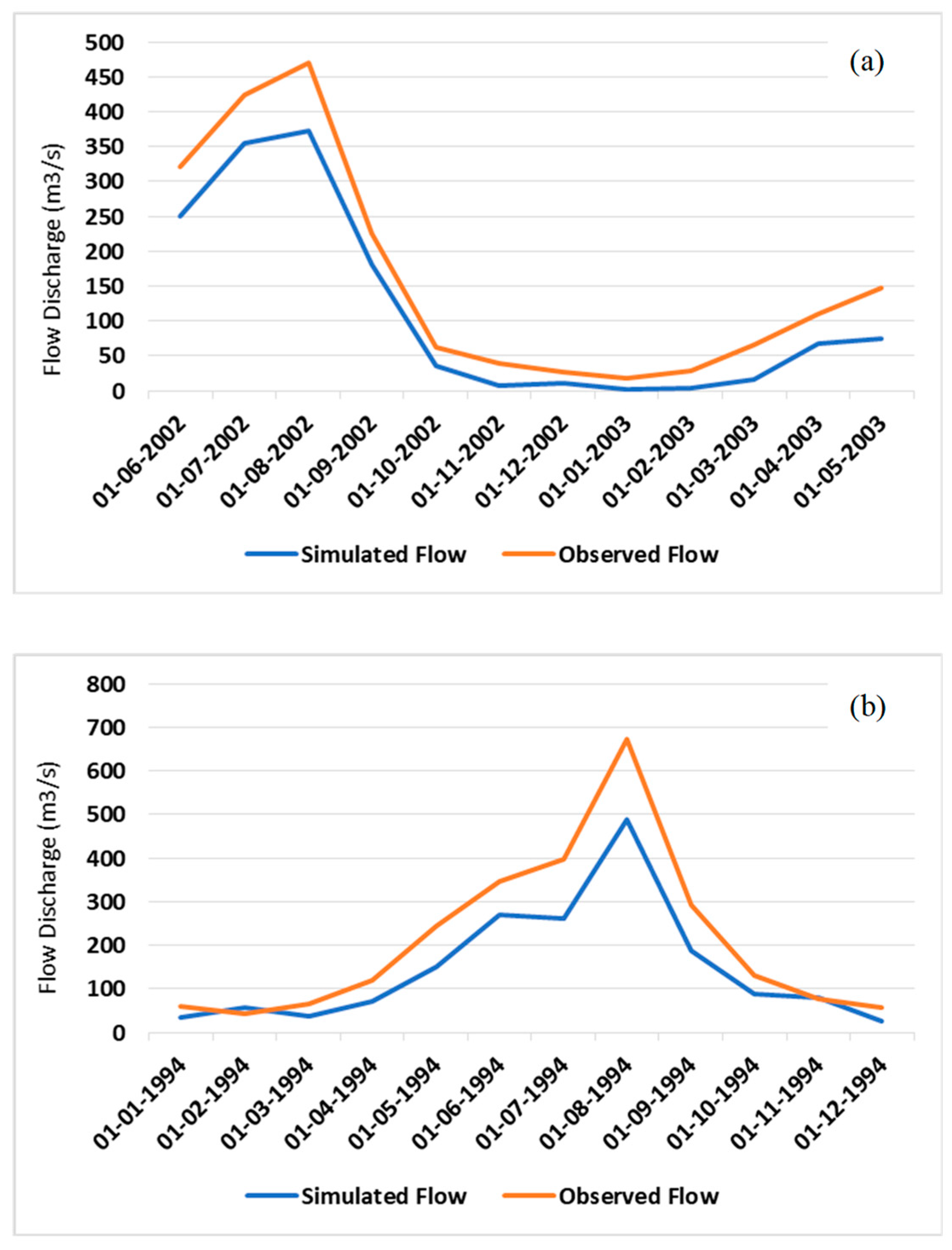
The SWAT+ model was calibrated using recorded streamflow at the Larji Hydroelectric Project outlet, identifying 12 parameters as the most sensitive ones affecting hydrological simulations. The calibrated streamflow and simulated flow in Figure 6 closely align the data with the observed flow throughout the period. Model performance was evaluated using statistical indices, demonstrating good agreement with an NSE of 0.88 and BIAS of 21.

The model validation revealed that the simulated and recorded data were closely aligned (NSE = 0.82, BIAS = 24).

The calibration process involved calibrating streamflow for monthly conditions through a trial-and-error method by adjusting the SWAT+ parameters’ values within their acceptable ranges to optimize the model. The calibration and validation process was conducted to predict annual water balance components like surface runoff, water yield, evapotranspiration, percolation rate, lateral flow, return flow, and daily precipitation.

The calibration and validation of the SWAT+ model for the Larji Hydroelectric Project have been significantly influenced by the sensitive parameters listed in

Table 3. Sensitive parameters.

Parameter Abbreviation	Value	Range
Base flow alpha factor ALPHA_BF	0.74	0–1
SCS runoff curve number for moisture condition II CN2	19.3%	35–95
Manning’s coefficient for channel CH N2	0.18	−0.01–0.3
Effective hydraulic conductivity in main channel CH K2	215	−0.01–500
Plant uptake compensation factor EPCO	0.80	0.01–1
Soil evaporation compensation factor ESCO	0.89	0.01–1
Surface runoff lag coefficient SURLAG	0.20	0–10
Groundwater revap coefficient GW_REVAP

. With the model yielding an NSE of 0.88 and 0.82 for calibration and validation, respectively, and BIAS values of 21 and 24, the importance of accurately determining sensitive parameters becomes evident. For instance, the surface runoff lag coefficient (SURLAG) stands at 0.74 within a range of 0–10, hinting at the watershed’s response time post-rainfall. Meanwhile, the groundwater revap coefficient (GW_REVAP) is 0.17, within its 0.02–0.2 range, offering insights into groundwater behavior. While not explicitly detailed in the table, other parameters, such as ALPHA_BF, CN2, CH N2, and CH K2, play fundamental roles in calibrating the hydrological behaviors. The alignment of observed and simulated data, shaped significantly by these sensitive parameters, emphasizes the SWAT+ model’s reliability for forecasting hydrological dynamics in the Larji Hydroelectric Project region.

The sensitivity analysis of the SWAT model based on the provided parameter data reveals valuable insights into the influence of each parameter on the model outputs. Among the parameters evaluated, the base flow alpha factor (ALPHA_BF) and the SCS runoff curve number for moisture condition II (CN2) show that significant sensitivity plays a crucial role in simulating base flow and affects the overall streamflow dynamics. The CN2 parameter exhibits sensitivity in the runoff simulation, reflecting the varying runoff potential for different moisture conditions.

Furthermore, the Manning’s coefficient for the channel (CH_N2), effective hydraulic conductivity in the main channel (CH_K2), plant uptake compensation factor (EPCO), soil evaporation compensation factor (ESCO), surface runoff lag coefficient (SURLAG), and groundwater revap coefficient (GW_REVAP) also contribute to the sensitivity of the SWAT model. These parameters, with their respective values falling within the specified ranges, impact the representation of channel roughness, hydraulic conductivity, plant water uptake, soil evaporation, surface runoff generation, and groundwater–surface water interactions.

Table 4. Simulated water balance components.

Hydrological Component	Annual Average
Surface Flow	231
Water Yield	236
Evapotranspiration	506
Potential Evapotranspiration	1839
Lateral Flow	4.95

shows simulated water balance components.

The Beas Basin, a crucial watershed area, is characterized by an intricate network of hydrological components. The simulation results highlight key features of the basin’s annual average hydrological behaviors. Surface flow emerges as a key component within the hydrological cycle of the basin, averaging 231 mm annually. This metric indicates the volume of water rapidly transported over the land surface to the nearest stream channel following a rainfall event. The significant surface flow is a testimony to the prevalent runoff-generating mechanisms within the watershed.

The water yield, another crucial element in the hydrological balance, is an annual average of 236 mm. Water yield represents the total amount of water the basin produces, including surface flow, groundwater flow, and any contribution from precipitation. This value reflects the capacity of the Beas Basin to provide water for various needs, including hydroelectric generation, irrigation, and ecological sustenance. Lateral flow, accounting for an average of 4.95 mm annually, suggests the presence of subsurface hydrological pathways. These subsurface flows can contribute significantly to streamflow, especially during dry periods.

Evapotranspiration (ET), which quantifies the amount of water transferred from the land to the atmosphere, averages 506 mm annually. This value encompasses water evaporated from the soil surface and transpired by plants, a significant component given the basin’s vegetative cover. This high ET value indicates the basin’s large demand for atmospheric moisture. Lastly, the potential evapotranspiration (PET), which signifies the amount of evaporation that would occur if a sufficient water source were available, is calculated to be 1839 mm annually. This value represents the climatic demand for water and underscores the important role of climatic factors in governing the basin’s hydrological processes.

3.2. Simulated Time Series of Flow Discharge and Sediment Flow

3.2.1. Flow Discharge

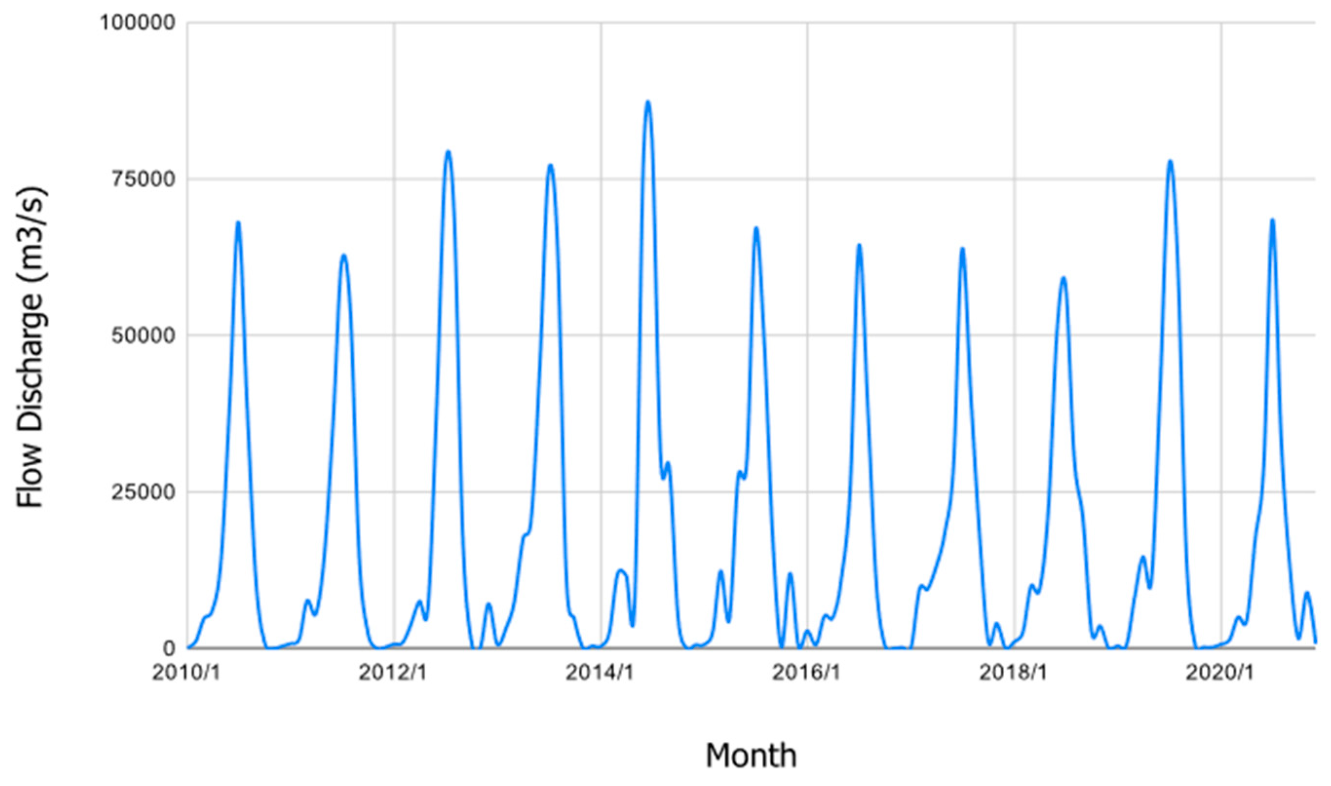
The temporal analysis of flow discharge in the Beas Basin (Figure 7), stretching from January 2010 to December 2022, reveals a complex interplay of seasonality and interannual variability. The analysis underlines a consistent pattern marked by pronounced seasonal oscillations.

During each year under review, the discharge pattern adheres to an annual rhythm. It is typically characterized by lower volumes during winter, particularly January and February. This is followed by a moderate increment in the spring months, notably in March and April. From May to August, the summer months witness a significant discharge surge due to the combined effect of snowmelt and monsoon precipitation, reaching an annual peak. Post-peak, the autumn months of September and October observe a reduction in discharge, which reaches its nadir during the subsequent winter months.

Certain years such as 2014 and 2020 showcased extreme discharge events. In June 2014, an unprecedented discharge value of 632 m³/s was recorded, potentially driven by exceptional precipitation or accelerated snowmelt. Similarly, July 2020 experienced a substantial peak discharge of 436 m³/s.

3.2.2. Sediment Discharge

Parallel to the flow discharge, the sediment discharge (Figure 8) also follows a similar annual rhythm. The sediment volumes tend to be lower during winter, followed by a gradual increase during spring. The summer months see a considerable increase in sediment discharge, primarily due to enhanced runoff from snowmelt and monsoon rains, marking the annual peak. The autumn months, however, witness a decline in sediment discharge, reaching the lowest point during the winter season.

In 2010, the sediment discharge initiated at a minimal 85.50 tons in January, and increased significantly, peaking at 68,100 tons in July. Following this peak, there was a consistent reduction, reaching a value of 334 tons by December. Comparable annual trends were observed in subsequent years, highlighting the consistent erosion–deposition cycle within the basin.

However, certain years, such as 2014 and 2020, demonstrated exceptional sediment discharge events. In June 2014, the sediment discharge reached an all-time high of 81,800 tons, potentially triggered by excessive precipitation or accelerated erosion. Similarly, July 2020 saw a substantial sediment discharge of 68,500 tons. In stark contrast, November 2021 registered virtually null sediment discharge, possibly due to reduced precipitation or erosion.

3.3. Spatial Distribution of Hydrological Component

3.3.1. Surface Runoff

Surface runoff is the water flow that occurs when excess stormwater, meltwater, or other sources of water flow over the Earth’s surface. The annual mean surface runoff for the entire basin reveals significant hydrological diversity inherent within this basin. A significant segment of the basin, accounting for a vast 7657 sq km and involving subbasins 7, 8, 9, 11, and 12, displays an annual mean surface runoff within the 44–128 mm range. This range suggests a relative consistency in the hydrological processes across this major part of the basin. Subbasins 3, 4, and 6 constitute another notable category, covering an area of 2799 sq km. In this region, the annual mean surface runoff rises, moving within a higher range of 129–471 mm. Subbasin 2 is particularly noteworthy due to its distinctive characteristics. Covering an area of 1419 sq km, this subbasin records a significantly higher annual mean surface runoff within the substantial range of 472–911 mm. The fact that this subbasin alone falls within this category indicates unique hydrological dynamics at work. Subbasins 1, 10, and 13 exhibit the least surface runoff on the other end. Spanning an area of 1619 sq km, these subbasins fall within the lowest range of 9–33 mm for the annual mean surface runoff.

The surface flow shown in

Table 5. Surface flow.

Subbasin	Surface Flow (in mm)
1	29.09
2	1164.47
3	225.16
4	258.84
5	43.16
6	471.12
7	82.96
8	67.22
9	74.57
10	8.82
11	88.46
12	127.83
13	9.23

, the direct water runoff on the surface, varies significantly across the subbasins. Subbasin 2 takes the lead with the highest surface flow, recording 1164.47 mm, signifying substantial surface runoff in this region. Subbasin 6 also demonstrates noteworthy surface flow, amounting to 471.12 mm, indicating its significant contribution to the hydrological dynamics of the watershed. Subbasin 3 follows closely with a surface flow of 225.16 mm, highlighting the importance of surface runoff in its hydrological processes. In contrast, Subbasin 10 exhibits the lowest surface flow among the subbasins, with a minimal 8.82 mm, emphasizing its limited role in surface runoff generation.

3.3.2. Water Yield

Water yield, a crucial component of the hydrological cycle, refers to the total amount of water that is produced from a catchment area. This typically includes all forms of surface and subsurface water flow that reach a particular point in a water body, often described as streamflow or runoff. Water yield is particularly significant for water resource management, as it provides essential information for applications such as irrigation planning, flood control, and the maintenance of ecological water requirements.

The analysis of water yield among the studied subbasins reveals significant variations. Subbasin 2 stands out with the highest water yield, recording a substantial runoff of 1182.32 mm, which suggests a region with significant surface water availability. Following closely is Subbasin 6, characterized by a water yield of 492.22 mm, reflecting its hydrologically active nature. Subbasin 3 also demonstrates a relatively high water yield of 229.27 mm, indicating its contribution to the overall runoff within the watershed. Conversely, Subbasin 10 exhibits the lowest water yield among the studied subbasins, with a mere 8.83 mm, indicating minimal surface runoff. This finding underscores potential water availability challenges in this particular area.

The spatial distribution of annual water yield shown in

Table 6. Water yield (in mm).

Subbasin	Water Yield (in mm)
1	29.62
2	1182.32
3	229.27
4	259.89
5	43.18
6	492.22
7	84.60
8	67.37
9	74.57
10	8.83
11	123.34
12	139.29
13	11.69

in the Beas Basin exhibits marked variation, falling within five distinct categories. The initial category ranges from 9 to 33 mm. This section, covering an area of 2799 sq km, records the minimum annual water yield among all categories. A significantly larger segment of the basin, spanning 7657 sq km, falls within the second category, which records an annual water yield of 33 to 139 mm. The third category is characterized by an annual water yield ranging from 140 to 260 mm. Collectively, these subbasins occupy an area of 1963 sq km, highlighting a moderate enhancement in the water yield. The fourth category is distinguished by an annual water yield ranging from 261 to 492 mm, which covers an area of 836 sq km. Lastly, the fifth category, spanning an area of 1419 sq km, presents a striking deviation from the rest of the basin, registering the highest annual water yield within the range of 493 to 1182 mm. The unique hydrological dynamics in this region underscore the potential for intensive water resource management.

3.3.3. Evapotranspiration

Evapotranspiration (ET) is the process through which water is transferred from the land to the atmosphere by evaporation from the soil and other surfaces and by transpiration from plants. Analyzing the spatial distribution of annual mean ET (

Table 7. Spatial distribution of mean annual ET.

Subbasin	Evapotranspiration (in mm)
1	679.48
2	273.17
3	710.57
4	614.64
5	641.13
6	440.62
7	460.15
8	418.10
9	656.40
10	621.65
11	519.55
12	478.12
13	431.59

) across our study area reveals distinct patterns reflecting the diverse hydrological phenomena within the basin.

The analysis of evapotranspiration, representing the combined water loss through evaporation and transpiration, reveals notable differences among the subbasins. Subbasin 2 reports the lowest evapotranspiration at 273.17 mm, indicating a substantial demand for water by both atmospheric and vegetative processes. Following closely, Subbasin 3 demonstrates significant evapotranspiration of 710.57 mm, underlining the area’s considerable water consumption by evapotranspiration. Subbasin 5 also experiences high evapotranspiration at 641.13 mm despite its relatively lower water yield, emphasizing the area’s significant atmospheric and vegetative water demand. In contrast, Subbasin 10 exhibits the lowest evapotranspiration among the studied subbasins, totaling 621.65 mm, suggesting a relatively lower demand for water by atmospheric and vegetative processes.

The analysis categorizes the basin into five primary groups based on the observed ET levels. One section of the basin, stretching over 6302 sq km and encapsulating a major part of our study area, shows an annual mean ET between 284 and 460 mm. This span suggests a steady level of evapotranspiration across this significant area. Meanwhile, the area spanning 1419 sq km presents an ET range of 273–283 mm. Although it covers a smaller section of the basin, this area holds a distinct hydrological character, manifesting relatively lower ET rates than other regions. In contrast, a high ET range of 657–711 mm is observed in the 2063 sq km area. This region, although not the largest, demonstrates significant evapotranspiration dynamics, potentially due to unique climatic and environmental conditions. An intermediate ET level, ranging from 461–520 mm, is observed in a 1283 sq km area, while a 3607 sq km section shows an ET range of 521–656 mm. These regions suggest different intensities of ET processes, highlighting the heterogeneity in the hydrological processes across the basin.

3.3.4. Lateral Flow

Lateral flow, or subsurface runoff, is a crucial aspect of the hydrological cycle. It denotes the horizontal movement of water in the soil layer, significantly shaping soil moisture distribution, nutrient transport, and the health of the wider watershed. Factors including rainfall intensity, soil properties, and land use patterns considerably influence lateral flow.

Spatial distribution of mean annual lateral flow (

Table 8. Spatial distribution of mean annual lateral flow.

Subbasin	Lateral Flow (in mm)
1	3.52
2	17.85
3	4.12
4	3.06
5	2.02
6	21.10
7	1.64
8	1.15
9	0.06
10	1.03
11	34.89
12	11.46
13	2.45

) reveals that lateral flow values are notably minimal in an area spanning 8438 sq km, ranging from 0 to 1 mm. This largest section of the studied region exhibits remarkable hydrological stability, which might result from factors such as lower rainfall intensity, high infiltration rates, or effective land management strategies that curtail excessive surface runoff. The next category is an area covering 2698 sq km, which exhibits slightly increased lateral flow rates, ranging from 2 to 4 mm. This increase may hint at distinct soil characteristics or heightened rainfall incidents. A region occupying 933 sq km presents lateral flow rates between 5 and 11 mm. This area might harbor specific hydrological attributes, such as denser vegetation cover or more clayey soil types, which tend to enhance lateral flows. A significantly larger lateral flow rate, falling between 12 and 21 mm, is observed in an area covering 2255 sq km. This increased rate might indicate higher rainfall or less permeable soil properties, favoring more horizontal water movement. The highest lateral flow levels, ranging from 22 to 35 mm, are evident in a smaller region of 350 sq km. Despite this region’s smaller size, its high lateral flow rate could be attributed to unique hydrogeological factors or regular occurrences of high-intensity rain events.

Lateral flow, the lateral movement of water within a subbasin, varies significantly among the subbasins. Subbasin 11 exhibits the highest lateral flow at 34.89 mm, indicating a significant lateral water movement within the subbasin. Subbasin 6 also shows considerable lateral flow at 21.10 mm, contributing to its hydrological complexity. Subbasin 1 has a moderate lateral flow of 3.52 mm, playing a minor role in its hydrological processes. In contrast, Subbasin 9 has the lowest lateral flow, with a mere 0.06 mm, suggesting limited lateral water movement within this region.

3.3.5. Soil Percolation

Percolation, the process by which water infiltrates the soil profile and replenishes groundwater resources, plays an essential role in the hydrological cycle. It influences soil moisture content and determines water availability for plant uptake and maintaining the water balance in a watershed. The spatial distribution of percolation (

Table 9. Spatial distribution of mean annual soil percolation.

Subbasin	Percolation (in mm)
1	12.46
2	573.28
3	171.35
4	22.68
5	0.74
6	46.57
7	15.52
8	14.97
9	3.30
10	0.39
11	202.05
12	149.18
13	28.67

) within the study area showcases substantial hydrological diversity. An area of 2878 sq km experiences minimal percolation rates, ranging from 0 to 3 mm. The limited percolation could be due to the prevalence of impermeable soils or minimal rainfall events, suggesting a hydrological balance in favor of surface or lateral flows over percolation.

The largest part of the study region, encompassing 7024 sq km, presents percolation rates between 4 and 29 mm. This substantial area could be characterized by soils with medium permeability or average rainfall events, balancing between runoff and percolation. A smaller region, covering 836 sq km, indicates elevated percolation rates within the range of 30 to 47 mm. Such a pattern might be a consequence of soil types with higher permeability or greater precipitation, potentially leading to increased groundwater recharge in this area. An area of 2517 sq km shows significantly higher percolation rates, between 48 and 202 mm. The highest percolation rates, ranging from 203 to 573 mm, are observed in a smaller area of 1419 sq km. These rates could suggest the presence of highly permeable soils or frequent intense rainfall events, leading to a predominance of percolation. The understanding of spatial percolation patterns is crucial in the management of soil water content, groundwater recharge, and overall watershed management. Such insights also offer significant value in predicting and mitigating the impacts of climate change on water availability.

Percolation, indicating the downward movement of water through the soil, exhibits variability among the subbasins. Subbasin 2 stands out with the highest percolation of 573.28 mm, suggesting substantial potential for groundwater recharge. Subbasin 4 also shows noteworthy percolation at 22.68 mm, contributing to groundwater replenishment in the area. Subbasin 6 demonstrates a substantial percolation of 46.57 mm, highlighting the role of subsurface water movement in its hydrological dynamics. In contrast, Subbasin 5 has the lowest percolation among the studied subbasins, with a minimal 0.74 mm, suggesting limited groundwater recharge potential in this region.

3.3.6. Potential Evapotranspiration

Potential evapotranspiration (PET) is a critical hydrological parameter that signifies the ability of the atmosphere to remove water from the surface through evaporation and plant transpiration processes. Variations in PET are influenced by factors such as temperature, humidity, wind speed, and solar radiation [7].

In the study area, the spatial distribution of PET (

Table 10. Spatial distribution of mean annual PET.

Subbasin	Potential Evapotranspiration (in mm)
1	2332.70
2	401.14
3	2192.26
4	2207.53
5	2389.30
6	624.84
7	1628.74
8	2264.62
9	2170.10
10	2456.67
11	1052.30
12	1216.18
13	1634.20

) is characterized by significant diversity, highlighting the different climatic and biophysical conditions present. A segment of the area, accounting for 2255 sq km, manifests a PET within the 401–625 mm range. This suggests an environment with relatively moderate atmospheric demand for water, likely driven by temperate climate conditions or specific vegetation characteristics. Another area, spanning 1283 sq km, exhibits a PET ranging from 626 to 1216 mm. This increase indicates a stronger atmospheric demand for water, possibly resulting from higher temperatures or lower humidity levels. The third category, covering an area of 1454 sq km, shows a PET within the range of 1217 to 1634 mm. Such elevated values suggest the presence of warm and dry climatic conditions, leading to a high demand for evaporation and transpiration. A significantly large portion of the study area, amounting to 7580 sq km, records a PET ranging from 1635 to 2265 mm. These high values indicate particularly warm and dry conditions, likely leading to intense evaporation and transpiration processes. Finally, an area of 2092 sq km exhibits the highest PET values, ranging from 2266 to 2457 mm. These exceptionally high values suggest extreme climatic conditions with a very high atmospheric demand for water.

The potential evapotranspiration, representing the maximum potential water loss to evaporation and transpiration under ideal conditions, varies notably among the subbasins. Subbasin 10 records the highest potential evapotranspiration, totaling 2456.67 mm, highlighting the area’s susceptibility to high water loss under ideal environmental conditions. In contrast, Subbasin 1 displays a substantial difference between actual evapotranspiration (679.48 mm) and potential evapotranspiration (2332.70 mm), signifying potential water stress conditions. Subbasin 3 demonstrates significant potential evapotranspiration of 2192.26 mm, underscoring the need to consider actual evapotranspiration to assess water availability accurately.

4. Discussion

The results presented in the previous sections provide valuable insights into the hydrological characteristics of the Beas Basin, as simulated by the SWAT+ model. The calibration and validation processes have demonstrated the model’s ability to accurately represent streamflow and other hydrological components, indicating a good performance. The statistical indices, such as the Nash–Sutcliffe efficiency (NSE) and BIAS, further confirm the model’s reliability in reproducing observed data. The sensitivity analysis of the model identified several key parameters that significantly influence the hydrological processes in the Beas Basin. Parameters related to base flow, runoff, channel characteristics, plant water uptake, soil evaporation, surface runoff lag, and groundwater–surface water interactions were particularly sensitive [32]. These findings highlight the importance of accurately estimating and prioritizing these parameters during model calibration to improve the representation of hydrological dynamics.

The detailed simulations and analysis of the SWAT+ model have unveiled the intricate hydrological dynamics prevailing within the Beas Basin. One of the standout aspects of this study is the model’s calibration using recorded streamflow at the Larji Hydroelectric Project outlet. This calibration has showcased the model’s precision and adaptability in recognizing and adjusting to sensitive parameters. Specifically, parameters such as the surface runoff lag coefficient (SURLAG) and groundwater revap coefficient (GW_REVAP) with values of 0.74 and 0.17, respectively, reveal the basin’s nuanced response mechanisms to various hydrological events, particularly precipitation [33].

We can quantitatively dissect the basin’s hydrological behavior by diving into the water balance components. For instance, the annual average surface flow of 231 mm, juxtaposed against the water yield of 236 mm, paints a quantitative picture of the balance between surface runoff and the total water available from the basin. This balance is paramount, serving various needs, from hydroelectric power generation to maintaining the basin’s ecological vitality. The lateral flow, albeit a smaller value of 4.95 mm, should not be overlooked, as it suggests potential subsurface pathways, crucial during periods of lower precipitation.

Evapotranspiration, a pivotal component in the water cycle, stands at an annual average of 506 mm in the Beas Basin. When we place this value against the potential evapotranspiration of 1839 mm, it becomes evident that the region has a massive climatic demand for water. This dynamic is further shaped by the basin’s vegetative cover, topography, and soil characteristics [34].

The temporal analysis, spanning 2010 to 2022, provides insights into the basin’s hydrological rhythm. While the seasonal oscillations are evident, anomalies like the extreme discharge events of 2014 and 2020 truly test the model’s predictive capabilities. These events, marked by discharges of 632 m³/s and 436 m³/s, respectively, suggest the model’s aptitude for capturing significant hydrological events based on historical data and sensitive parameter adjustments [35].

The spatial analysis further delves into the heterogeneity of the basin. Different subbasins, like subbasin 2 with its high surface flow of 1164.47 mm and water yield of 1182.32 mm, contrast starkly with subbasin 10, which exhibits minimal values. These variations are emblematic of the diverse hydrological, geological, and climatic conditions inherent within the basin. Furthermore, potential evapotranspiration values, such as the 2456.67 mm in subbasin 10, emphasize areas with pronounced atmospheric water demand. These insights are invaluable for future water resource planning, especially in the face of potential climatic shifts.

5. Conclusions

This study presents an in-depth exploration of the hydrological dynamics within the Beas Basin using the Soil and Water Assessment Tool (SWAT+), aiming to improve our understanding of the region’s hydrological characteristics and their implications for water resource management. The calibration and validation of the SWAT+ model demonstrated reliable performance in simulating the hydrological processes within the Beas Basin. The high Nash–Sutcliffe efficiency (NSE) values (0.88 for calibration and 0.82 for validation) and acceptable biases affirm the model’s robustness in reflecting the basin’s hydrological dynamics. The calibrated SWAT+ model facilitated an accurate simulation of crucial hydrological components, including surface runoff, water yield, evapotranspiration, potential evapotranspiration, and lateral flow. The annual averages of these components underline the Beas Basin’s intricate hydrological network and its responsiveness to climatic factors and terrain attributes. The temporal analyses of flow and sediment discharge revealed a predictable yet complex interplay of seasonality and interannual variability, emphasizing the basin’s susceptibility to extreme discharge events due to precipitation and snowmelt anomalies. The spatial distribution of surface runoff and water yield highlights the significant hydrological diversity within the Beas Basin. These spatial patterns can be associated with various factors, such as vegetation, soil properties, topography, and climatic conditions, which shape the hydrological behaviors in different basin parts. This study provides valuable insights into the hydrological regime of the Beas Basin, contributing to the broader understanding of the region’s water resource potential and sustainability. The findings could significantly influence water resource planning, flood control, agricultural management, and ecological conservation within the basin. This study also underscores the utility of tools like SWAT+ in hydrological assessment and water management strategies. The implications of this modeling exercise hold significant weight for water resource managers, especially in climate change. Through an in-depth analysis of the Beas Basin’s hydrological components using the SWAT+ model, calibrated and validated with sensitivity considerations, this study offers a nuanced comprehension of its intricate dynamics. This understanding translates into actionable benefits for managers, as it unveils tailored insights for resource allocation and management strategies in various subbasins. It also enhances decision-making accuracy through the spatial distribution of key water balance components. In the face of climate uncertainty, the model’s parameter sensitivity ensures continued reliability, enabling managers to formulate adaptive strategies that account for evolving climatic conditions. Ultimately, this modeling effort advances knowledge of the basin’s hydrology and equips managers with a potent tool to navigate climate-induced challenges, securing water resource sustainability and basin resilience. Future research can build upon this work to further explore other water cycle components, such as groundwater dynamics, soil moisture patterns, and their linkages with climate change scenarios.

References

1. Singh, A.P.; Bhakar, P. Development of groundwater sustainability index: A case study of western arid region of Rajasthan, India. Environ. Dev. Sustain. 2021, 23, 1844–1868. [Google Scholar] [CrossRef]
2. Kumar, P.; Avtar, R.; Dasgupta, R.; Johnson, B.A.; Mukherjee, A.; Ahsan, M.N.; Nguyen, D.C.; Nguyen, H.Q.; Shaw, R.; Mishra, B.K. Socio-hydrology: A key approach for adaptation to water scarcity and achieving human well-being in large riverine islands. Prog. Disaster Sci. 2020, 8, 100134. [Google Scholar] [CrossRef]
3. Shyam, M.; Meraj, G.; Kanga, S.; Farooq, M.; Singh, S.K.; Sahu, N.; Kumar, P. Assessing the Groundwater Reserves of the Udaipur District, Aravalli Range, India, Using Geospatial Techniques. Water 2022, 14, 648. [Google Scholar] [CrossRef]
4. Meraj, G. Assessing the Impacts of Climate Change on Ecosystem Service Provisioning in Kashmir Valley India. Ph.D. Thesis, Suresh Gyan Vihar University, Jaipur, India, 2021. [Google Scholar]
5. Meraj, G.; Singh, S.K.; Kanga, S.; Islam, M.N. Modeling on comparison of ecosystem services concepts, tools, methods and their ecological-economic implications: A review. Model. Earth Syst. Environ. 2021, 8, 15–34. [Google Scholar] [CrossRef]
6. Upadhyay, M.K.; Majumdar, A.; Barla, A.; Bose, S.; Srivastava, S. An assessment of arsenic hazard in groundwater–soil–rice system in two villages of Nadia district, West Bengal, India. Environ. Geochem. Health 2019, 41, 2381–2395. [Google Scholar] [CrossRef]
7. Galkate, R.V.; Yadav, S.; Pandey, R.P.; Negm, A.M.; Yadava, R.N. An Overview: Water Resource Management Aspects in India. Water Qual. Assess. Manag. India 2022, 16, 29–55. [Google Scholar]
8. Bera, A.; Meraj, G.; Kanga, S.; Farooq, M.; Singh, S.K.; Sahu, N.; Kumar, P. Vulnerability and Risk Assessment to Climate Change in Sagar Island, India. Water 2022, 14, 823. [Google Scholar] [CrossRef]
9. Singh, L.K.; Jha, M.K.; Chowdary, V.M. Assessing the Accuracy of GIS-Based Multi-Criteria Decision Analysis Approaches for Mapping Groundwater Potential. Ecol. Indic. 2018, 91, 24–37. [Google Scholar] [CrossRef]
10. Thapa, R.; Gupta, S.; Guin, S.; Kaur, H. Assessment of Groundwater Potential Zones Using Multi-Influencing Factor (MIF) and GIS: A Case Study from Birbhum District, West Bengal. Appl. Water Sci. 2017, 7, 4117–4131. [Google Scholar] [CrossRef]
11. Owolabi, S.T.; Madi, K.; Kalumba, A.M.; Orimoloye, I.R. A Groundwater Potential Zone Mapping Approach for Semi-Arid Environments Using Remote Sensing (RS), Geographic Information System (GIS), and Analytical Hierarchical Process (AHP) Techniques: A Case Study of Buffalo Catchment, Eastern Cape, South Africa. Arab. J. Geosci. 2020, 13, 1184. [Google Scholar] [CrossRef]
12. Tolche, A.D. Groundwater Potential Mapping Using Geospatial Techniques: A Case Study of Dhungeta-Ramis Sub-Basin, Ethiopia. Geol. Ecol. Landsc. 2021, 5, 65–80. [Google Scholar] [CrossRef]
13. Zghibi, A.; Mirchi, A.; Msaddek, M.H.; Merzougui, A.; Zouhri, L.; Taupin, J.D.; Chekirbane, A.; Chenini, I.; Tarhouni, J. Using Analytical Hierarchy Process and Multi-Influencing Factors to Map Groundwater Recharge Zones in a Semi-Arid Mediterranean. Water 2020, 12, 2525. [Google Scholar] [CrossRef]
14. Rather, M.A.; Meraj, G.; Farooq, M.; Shiekh, B.A.; Kumar, P.; Kanga, S.; Singh, S.K.; Sahu, N.; Tiwari, S.P. Identifying the Potential Dam Sites to Avert the Risk of Catastrophic Floods in the Jhelum Basin, Kashmir, NW Himalaya, India. Remote Sens. 2022, 14, 1538. [Google Scholar] [CrossRef]
15. Lahon, D.; Sahariah, D.; Debnath, J.; Nath, N.; Meraj, G.; Farooq, M.; Kanga, S.; Singh, S.; Chand, K. Growth of water hyacinth biomass and its impact on the floristic composition of aquatic plants in a wetland ecosystem of the Brahmaputra floodplain of Assam, India. PeerJ 2023, 11, e14811. [Google Scholar] [CrossRef] [PubMed]
16. Nath, N.; Sahariah, D.; Meraj, G.; Debnath, J.; Kumar, P.; Lahon, D.; Chand, K.; Farooq, M.; Chandan, P.; Singh, S.K.; et al. Land Use and Land Cover Change Monitoring and Prediction of a UNESCO World Heritage Site: Kaziranga Eco-Sensitive Zone Using Cellular Automata-Markov Model. Land 2023, 12, 151. [Google Scholar] [CrossRef]
17. Kanga, S.; Meraj, G.; Johnson, B.A.; Singh, S.K.; PV, M.N.; Farooq, M.; Kumar, P.; Marazi, A.; Sahu, N. Understanding the Linkage between Urban Growth and Land Surface Temperature—A Case Study of Bangalore City, India. Remote Sens. 2022, 14, 4241. [Google Scholar] [CrossRef]
18. Meraj, G.; Romshoo, S.A.; Yousuf, A.R.; Altaf, S.; Altaf, F. Assessing the influence of watershed characteristics on the flood vulnerability of Jhelum basin in Kashmir Himalaya. Nat. Hazards 2015, 77, 153–175. [Google Scholar] [CrossRef]
19. Sud, A.; Kanga, R.; Singh, S.K.; Meraj, G.; Kanga, S.; Kumar, P.; Ramanathan, A.L.; Sudhanshu, S.; Bhardwaj, V. Simulating Groundwater Potential Zones in Mountainous Indian Himalayas—A Case Study of Himachal Pradesh. Hydrology 2023, 10, 65. [Google Scholar] [CrossRef]
20. Fayaz, M.; Meraj, G.; Khader, S.A.; Farooq, M. ARIMA and SPSS statistics based assessment of landslide occurrence in western Himalayas. Environ. Chall. 2022, 9, 100624. [Google Scholar] [CrossRef]
21. Fayaz, M.; Meraj, G.; Khader, S.A.; Farooq, M.; Kanga, S.; Singh, S.K.; Kumar, P.; Sahu, N. Management of landslides in a rural–urban transition zone using machine learning algorithms—A case study of a National Highway (NH-44), India, in the Rugged Himalayan Terrains. Land 2022, 11, 884. [Google Scholar] [CrossRef]
22. Rehman, A.; Song, J.; Haq, F.; Mahmood, S.; Ahamad, M.I.; Basharat, M.; Sajid, M.; Mehmood, M.S. Multi-hazard susceptibility assessment using the analytical hierarchy process and frequency ratio techniques in the Northwest Himalayas, Pakistan. Remote Sens. 2022, 14, 554. [Google Scholar] [CrossRef]
23. Meraj, G.; Farooq, M.; Singh, S.K.; Islam, M.N.; Kanga, S. Modeling the sediment retention and ecosystem provisioning services in the Kashmir valley, India, Western Himalayas. Model. Earth Syst. Environ. 2022, 8, 3859–3884. [Google Scholar] [CrossRef]
24. Gad, M.; El-Safa, M.M.A.; Farouk, M.; Hussein, H.; Alnemari, A.M.; Elsayed, S.; Khalifa, M.M.; Moghanm, F.S.; Eid, E.M.; Saleh, A.H. Integration ofWater Quality Indices and Multivariate Modeling for Assessing Surface Water Quality in Qaroun Lake, Egypt. Water 2021, 13, 2258. [Google Scholar] [CrossRef]
25. Kahal, A.; El-Sorogy, A.S.; Alfaifi, H.; Almadani, S.; Ghrefat, H.A. Spatial distribution and ecological risk assessment of the coastal surface sediments from the Red Sea, northwest Saudi Arabia. Mar. Pollut. Bull. 2018, 137, 198–208. [Google Scholar] [CrossRef] [PubMed]
26. Saber, A.; Roohollah, N.; Mohammad, R.V.N.; Majid, H.; Salman, S.; Fardin, G.R.; Mohsen, M. Alarming carcinogenic and non-carcinogenic risk of heavy metals in Sabalan dam reservoir, Northwest of Iran. Environ. Pollut. Bioavailab. 2021, 33, 278–291. [Google Scholar]
27. Sehad, M.; Ameur, S. A multilayer perceptron and multiclass support vector machine based high accuracy technique for daily rainfall estimation from MSG SEVIRI data. Adv. Space Res. 2020, 65, 1250–1262. [Google Scholar] [CrossRef]
28. Kinouchi, T. Synergetic application of GRACE gravity data, global hydrological model, and in-situ observations to quantify water storage dynamics over Peninsular India during 2002–2017. J. Hydrol. 2021, 596, 126069. [Google Scholar]
29. Lazri, M.; Labadi, K.; Brucker, J.M.; Ameur, S. Improving satellite rainfall estimation from MSG data in Northern Algeria by using a multi-classifier model based on machine learning. J. Hydrol. 2020, 584, 124705. [Google Scholar] [CrossRef]
30. Belmahdi, F.; Lazri, M.; Ouallouche, F.; Labadi, K.; Absi, R.; Ameur, S. Application of Dempster Shafer theory for optimization of precipitation classification and estimation results from remote sensing data using machine learning. Remote Sens. Appl. Soc. Environ. 2023, 29, 100906. [Google Scholar] [CrossRef]
31. Castillo Botón, C.; Casillas Pérez, D.; Casanova- Mateo, C.; Ghimire, S.; Cerro-Prada, E.; Gutierrez, P.A.; Deo, R.C.; Salcedo Sanz, S. Machine learning regression and classification methods for fog events prediction. Atmos. Res. 2022, 272, 106157. [Google Scholar] [CrossRef]
32. Belghit, A.; Lazri, M.; Ouallouche, F.; Labadi, K.; Ameur, S. Optimization of One versus All-SVM using Ada Boost algorithm for rainfall classification and estimation from multispectral MSG data. Adv. Space Res. 2023, 71, 946–963. [Google Scholar] [CrossRef]
33. Goshime, D.W.; Haile, A.T.; Absi, R.; Ledésert, B. Impact of water resource development plan on water abstraction and water balance of Lake Ziway, Ethiopia. Sustain. Water Resour. Manag. 2021, 7, 36. [Google Scholar] [CrossRef]
34. Kim, S.; Yang, D.S.; Kim, Y.S. Distribution of metal contamination and grain size in the sediments of Nakdong River, Korea. Environ. Monit. Assess. 2020, 192, 502. [Google Scholar] [CrossRef] [PubMed]
35. Petrella, E.; Raimondo, M.; Chelli, A.; Valentino, R.; Severini, E.; Diena, M.; Celico, F. Processes and factors controlling the groundwater flow in a complex landslide: A case study in the Northern Italy. Hydrol. Process. 2023, 37, e14891. [Google Scholar] [CrossRef]
Figure 1. Location map of the study area. The colours represent the elevations ranging from 200 to 6000 m asl. More description is provided in Figure 2.
Water 15 03338 g001
Figure 2. Methodology flowchart.
Water 15 03338 g002
Figure 3. Topography of the Beas basin.
Water 15 03338 g003
Figure 4. LULC Map of Beas Basin.
Water 15 03338 g004
Figure 5. Soil texture of Beas Basin.
Water 15 03338 g005
Figure 6. Simulated vs. observed flow at (a) Larji Hydroelectric Plant (b) Mahadev Hydroelectric Plant.
Water 15 03338 g006
Figure 7. Simulated hydrograph from 2010 to 2020.
Water 15 03338 g007
Figure 8. Sedimentation discharge time series from 2010 to 2020.
Water 15 03338 g008