Operation and Maintenance Cost of Water Management Systems: Analysis and Optimization

Abstract

The analysis and optimization of the operational and maintenance costs of water management systems is one of the key issues of their exploitation. This article presents a general model, supported by specially designed software, able to process the analysis of exploitation costs of multistate renewable systems. The proposed model allows for the consideration of costs related to preventive inspections and repairs and additional reliability associated costs, such as costs of the system in a state of deteriorated reliability and financial losses related to reduced serviceability of the system or a lack of rendering of services. By means of a multistate approach to the reliability analysis, the model allows for the determination of the level corresponding to the appropriate reliability state that, if exceeded, should result in undertaking the repair of the system. In this study, the MATLAB 9.13 (R2022b) environment was used for simulation and estimation of the costs of system maintenance and repairs according to the proposed model. The article presents the results of the optimization of exploitation and repair costs of water management systems, allowing the estimation of the optimal period between regular inspections while maintaining the safe operation of the system. The model and software proposed can be of assistance in supporting the decision process of maintenance planning for water management systems.

1. Introduction and Literature Review

Water management systems are one of the essential infrastructures impacting civilian population livability [1,2]. Water demand generated by communities and industries keeps growing [3,4]; the growth of demand is additionally accelerated by the continuous expansion of urban centers [5]. The systems carry out a number of key tasks like providing adequate sanitary conditions, distributing drinking water of appropriate quality, drainage of urban areas, protection against flooding, supplying water for agriculture, and many others. The sustainability of water management systems is additionally impacted by the decline in freshwater sources caused by climate variability and recent changes in climate [3,6]; that is why effective administration is one of the crucial aspects determining their maintenance at the relevant level. Freshwater systems are also exposed to various external elements that interfere with their performance, like temperature fluctuations, pressure changes, and tectonic movements. Water supply systems, especially their underground components, are recognized as being unable to be appropriately resistant to critical external disruptions [7,8,9,10], which results in a continuous necessity for the implementation of innovative solutions. All entities involved in freshwater distribution are then forced to continuously develop and apply modern methods of management and maintenance of operational continuity [3,4]. The adoption of new solutions and technologies entails an increase in the technical complexity of the systems [5] and, consequently, increases the costs of their functioning and maintenance [11,12,13,14]. Water management systems, because of the continuous necessity for adapting to new challenges, require uninterrupted significant investments [5]. Therefore, one of the key issues in the management of water systems is ensuring their uninterrupted functional continuity, connected to proper efficiency and reliability, at the lowest possible operating costs.

There are several research initiatives worldwide related to ensuring the respective quality and reliability of water distribution systems. Research works concern both the predicted growth of the population’s demand for fresh water, especially in urban centers, and the simultaneous increase in water scarcity. The activities are carried out in numerous fields. A number of studies are related to the more efficient use of fresh water [3,15,16]. They focus mainly on reducing non-revenue water amounts, as it has been estimated that between 30 and 40% of the total water supply is non-revenue water [3,17]. Investigations in this field are concentrated on the conservation of water and appropriate water demand management [6]. Another important issue concerning improving the efficiency of water management systems is wastewater reuse [18,19]. There are investigations highlighting the reuse of wastewater as one of the most important topics within water management systems [20,21,22]. These investigations result in the construction of models of the water resource cycle and water pollutant flow. The models help to improve the quality of the water and water resource allocation and to evaluate water utilization and technologies for purification [23,24]. The optimization of water supply networks is a consequent research field aiming to reflect both design and operation problems, resulting in a flow and pressure distribution that satisfies customer demands and, on the other hand, minimizes operational costs [25]. There are also works aiming to include carbon emission costs in the design and operation of water networks [5]. The results are multiobjective models using objectives in the analysis of life cycle costs, consumption of energy, greenhouse gas emissions, and consumption of resources [26]. Algorithms for minimizing the costs of pumping are another study direction, as the costs of energy consumed by pumps are a significant segment of the overall operational costs of systems of water supply [11]. Works carried out on this topic cover optimization models for planning of pump operations, reflecting hydraulic restrictions together with other operational and physical constraints [27,28,29]. Other studies examine the transformation of existing water distribution systems in order to improve management of urban runoffs and rainwaters [7]. These transformations are leading to the implementation of systems that are able to deliver a wide range of environmental, socioeconomic, and ecological services and benefits, contributing crucially to the sustainability of urban areas [30,31,32,33]. Furthermore, there is research covering the integration of different sectors of water systems [1,34] aiming to project integrated urban water management systems. The works concern strategic decision-making, multicriteria decision analysis, sensitivity and uncertainty analyses, and exploration of alternative water supplies [35,36,37].

An important segment of research related to fresh water distribution systems is composed of studies on cost optimization of systems. A number of studies concern the cost–benefit analysis of the implementation of rainwater collection systems [38]. One of the issues of concern in this field is the analysis of the cost efficiency of such systems in urban areas of high density [39]. Other works concern investigating the balance between investment costs of system installation and the benefits accrued from collected rainwater use [38]. There are also studies on the analysis of the reliability and costs of rainfall collection systems carried out by investigating the performance of the systems and analysis of life-cycle costs [40]. The obtained outcomes estimate the reliability of the system using average yearly rainfall data at any location [41]. The cost–benefit analysis of the methods of leakage reduction is another field of water supply systems optimization. This optimization is carried out by means of sensitivity and uncertainty analyses leading to the determination of appropriate leakage reduction methods including district metering, reduction in pressure, and renovation of pipes [42]. Several investigations have also been carried out regarding multiobjective optimization of water management systems, taking into account total cost, reliability, and quality of the water [43]. Another issue in water supply infrastructure optimization is concerned with reducing costs and impact on the environment. This approach focuses on decreasing the amount of supplied influents and the consumption of resources and electricity [44]. Estimating economic benefits and costs of interventions that improve access to water distribution facilities is a successful approach to water supply system cost optimization by means of time saved due to improved access to sanitation and water services [45].

There are various approaches for determining the optimal strategy for system maintenance and repair. One of these approaches aims to maximize the system’s lifetime and its reliability at a particular operation time [46]. The aim of this approach is to determine the optimal reassignment time and strategy to ensure the balance of a system with multistate components for the entire operation time. There is also research focusing on maintenance optimization through minimization of the expected maintenance and repair cost for repairable systems [47,48,49]. Zhao et al., in [48], proposed an opportunistic maintenance strategy for a series system to minimize the expected average cost per time unit in the long run. Peng and Feng, in [49], used the Markov decision process for modelling condition-based maintenance. More specifically, the authors used the Gaussian process to describe the system condition and to model the state transition of a system. The objective of their research was to optimize the threshold of system condition that minimizes the maintenance cost for a nonrepairable system, considering corrective and preventive actions [49]. Other studies [50,51] concerned the management and planning of system maintenance and operating, stating that all additional reliability associated costs have to be included in the analysis of a system’s total life cycle costs. The problem of analysis of the total costs of system maintenance and its cost optimization is particularly complicated for multistate systems. Lisnianski et al. [50] indicated that reliability associated costs for repairable multistate systems usually are crucial in cost analysis of their maintenance and operation. For a certain type of multistate system, such as water management systems, reliability states are closely related to system performance and efficiency of system operation, and additional cost can be associated with the efficiency or the quality of services provided [52]. In this context, the problem of optimization of system maintenance and operation costs can be expressed as a function of system reliability and efficiency, where the objective is to find the system maintenance strategy that minimizes the total cost under uninterrupted and reliable system operation, providing high efficiency [53]. The authors of [54] highlighted the challenge presented by predicting the need for corrective and repair actions that reduce cost while maintaining the quality of systems and assets.

This paper presents a general model for water management system costs analysis and estimation along with software created for and dedicated to these purposes. We propose a multistate approach to the system degradation description that allows for the comparison of different strategies, including perfect and various kinds of imperfect repairs. The multistate approach to reliability analysis of technical systems, associated with the analysis of exploitation and repair costs of regularly inspected systems, is an innovative contribution to studies on analysis and optimization of system maintenance costs. The association, in the context of preventive and corrective maintenance, carried out during scheduled inspections, allows for the determination of the reliability state of the system which, if exceeded, results in conducting repairs during inspection. The analysis of the relations of the total exploitation and repair costs to various strategies of maintenance management and different inspections intervals allows for the determination of the optimal strategy of conducting repairs and maintenance (and the optimal interval time between inspections). In this manner, we can seek an optimal strategy that minimizes the cost of a system’s maintenance while satisfying safety requirements corresponding to the system’s reliability level. Such an approach has never been proposed for the purpose of optimization of the exploitation and repairs of multistate systems, in particular water management systems. To analyze and optimize the costs of system maintenance and repairs, an application was created in order to simulate the costs with use of the MATLAB environment.

The main purpose of this paper is to solve the problem of optimizing the costs of exploitation and repairs of a water management system by means of appropriate scheduling of preventive, corrective, and repair actions. The objective of our research is to find the optimal interval between inspections which can minimize the maintenance and repair cost for the system, assuming that it is a multistate system. The proposed simulation application is based on a maintenance and repair strategy provided by the user as input data. By using this application, it is possible to compare different repair strategies, as shown in Section 4. The presented approach to the analysis of maintenance and repair costs takes into account the degradation process of the system. This process has an influence on its maintenance strategy and repair planning. By means of taking into account the reliability parameters of the system and applying a multistate approach to describe its degradation, we decide whether at the moment of planned inspection the corrective actions should be carried out depending on the system’s predicted reliability state. Consequently, by comparing the cost of system maintenance and repair to different values of inspection intervals, the main goal of our approach is to find the optimal inspection interval that allows for the minimization of maintenance and repair costs per time unit. The proposed model, supported by the created application, is applied to analyze the operation and repair costs for the water management system and to determine a maintenance and repair strategy, minimizing its total costs.

Our model, by taking into consideration the so-called “static cost” for each system state, enables one to include, in addition to the basic costs of repairs and inspections, costs associated with the system remaining in a worse state, e.g., reduced system efficiency, performance, or safety. In particular, apparently lower inspection and repair costs within a certain exploitation period can generate other costs associated with exploitation of the system and emerging from its reduced efficiency. In such a situation, a completely different strategy of inspection and repair scheduling, and of the system’s maintenance in general, can appear as more beneficial. Enhanced discussion on how the various “static costs” can influence determining the appropriate strategy of repairs, minimizing the total costs of system exploitation and repairs per time unit, is introduced in Section 4.

2. Methodology

2.1. Description of Multistate Approach Model

We propose a multistate approach for the analysis of a system’s reliability and assume the system is degrading over time. We consider a multistate system in which the individual reliability states of the system and its components correspond to their levels of degradation and aging [55,56,57]. By “State 1”, we denote a state of full system reliability where the system can be described as “as good as new”, and subsequent states are marked with 2, 3, …, ω. Depending on the number of specified reliability states, we assume that “State ω” is a state of complete degradation (damage to the system) in which the system cannot function. In the proposed multistate approach, the system, after leaving the state of “as good as new”, generally has worse reliability parameters. Thus, time T(2), indicating that the system is in reliability State 2, can follow a different distribution than time T(1), indicating that a system is in the best reliability state. By T(j), we denote a random variable representing the lifetime of the system in reliability state j, where j = 1, 2, …, ω.

In this paper, we apply the proposed multistate approach to reliability analysis and maintenance optimization of a water management system. Further, assuming that this system, at the initial moment of analysis, is in the state of “as good as new”, we define random variables T_sub({1, 2, …, j}) representing the system’s lifetime in reliability state subsets {1, 2, …, j}, where j = 1, 2, …, ω − 1.

With these notations, T_sub({1}), T_sub({1,2}), and T_sub({1,2,3}) denote, respectively, the times of the system being in reliability state subsets {1}, {1,2}, and {1,2,3}. It can be observed that $T_{sub}\left(\left\{1\right\}\right){\le T}_{sub}\left(\left\{\mathrm{1,2}\right\}\right){\le \cdots \le T}_{sub}\left(\{\mathrm{1,2},\dots ,\omega -1\}\right)$, where T_sub({1, 2, …, ω − 1) represents the system’s lifetime, i.e., the time from the state of “as good as new” until total failure. These random variables can utilize different distributions, e.g., the Weibull distribution, and in the simulation program, we refer to that situation as the “Shock Degradation Mode” due to the possibility of transition from a given state to any worse reliability state, including the state of the system’s failure.

One of the basic reliability characteristics that characterizes a system’s degradation process is failure intensity. In the case of a multistate approach, intensities of departure from individual reliability states or reliability state subsets can be considered. In our proposed multistate approach model, the distribution of a system’s lifetimes in the reliability state subsets corresponds to intensities of departure from the subsets of reliability states. Consequently, the degradation intensity, denoted by λ_j, corresponds to the intensity of system departure from the subset of reliability states {1, 2, …, j}, where j = 1, 2, …, ω − 1.

De Jonge et al. [58] consider perfect repairs and assume that both corrective and preventive maintenance make the system “as good as new”. The authors model a system deterioration process using a homogeneous gamma process. Van der Weide and Pandey [59] present an analytical model for evaluating the maintenance cost of engineering systems, including periodic inspections and condition-based preventive maintenance. They evaluate the cost rate as a function of inspection cost, maintenance, and unavailability. The authors highlight differences in the approach to maintenance cost evaluation for systems characterized by latent failures and self-announced failures. In the reliability analysis of renewable systems, when modelling their maintenance and estimating maintenance costs, the characteristics of system failures and information about them are of key importance. That is, whether failures are automatically detected (so-called self-announced failures, allowing the immediate reparation of the system) or the information about failures is hidden. In the latter case, a failure is not immediately visible (so-called latent failures), and therefore the failures can only be detected and repaired during a system’s inspections. Such classification of failure type in terms of maintenance and repair planning for a system is illustrated in Figure 1.

In the proposed general model, we consider several aspects of a maintenance and repair strategy for multistate systems:

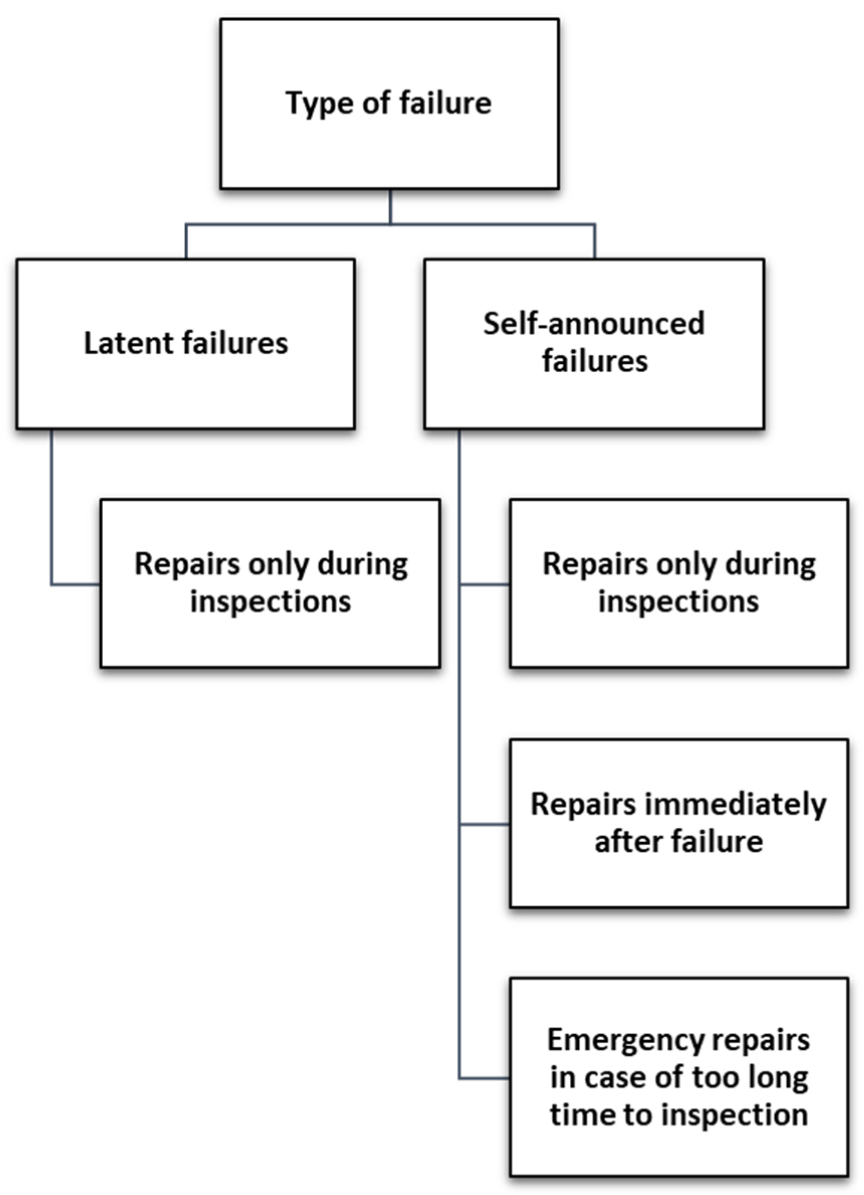
• Perfect/imperfect repairs: every repair leaves the system in the state of full reliability/it is possible to carry out a partial repair (leaving the system in a better state, but not necessarily “as good as new”).
• Always repair/custom repair objectives: every inspection finding the system in a state worse than State 1 results in a repair/for certain states; it is allowed to wait for further deterioration instead of implementing repair actions right away.
• Repairs only during inspections/possibility of emergency repairs: the state of the system is assessed only during scheduled inspections/after certain conditions are met; it is possible to request unscheduled emergency repair.

In particular, to make emergency repairs possible, it is crucial that a certain degree of deterioration is detectable without inspections (self-announced). If the system reaches such a state and the time before the next inspection is too long, an unscheduled repair can be conducted, possibly with a certain delay and additional costs. In this paper, we assume that only perfect repairs are possible and focus on minimizing the maintenance cost by optimizing the interval between inspections, adjusting the repair objectives and considering whether emergency repairs can be performed or not.

2.2. System Maintenance Cost and Its Optimization

In the model, we make several assumptions regarding the inspections. First, they occur at regular intervals. Second, they do not interfere with the system operation, and therefore their durations are negligible (or we can just include such duration as a part of the interval between inspections). For convenience, let us assume that the dividing point between two adjacent cycles is the end of the inspection at which the repair decision is made. Therefore, the length of each cycle can be expressed as an integer multiple of the interval duration between successive inspections.

We denote the number of production cycles by n. The length of the ith cycle, where i = 1, 2, …, n, can be expressed by formula

$$T_{C_i}=T_{R_F}+{\sum }_{j=1}^{\omega }{T}_{C_i}\left(j\right)=N_i{T}_B,$$

(1)

where $T_{R_F}$ is the recovery time from the state the system was in at the beginning of cycle to the state of “as good as new”, in the case of perfect repairs, or to another better reliability state in the case of imperfect repairs; $T_{C_i}\left(j\right)$ is the time during which the system was in the jth, j = 1, 2, …, ω, reliability state during the ith cycle, i.e., between the end of repair and the end of a given cycle, where i = 1, 2, …, n; $T_B$ is the length of the interval between successive inspections; and $N_i$ is the number of scheduled inspections during the ith cycle.

Note that depending on the repair objectives, some values of variables $T_{C_i}\left(j\right)$ representing the time of the system being in reliability states can equal zero. For example, if the system is repaired to State 2 and the next repair is undertaken in State 3, then, during this cycle, $T_{C_i}\left(4\right)=T_{C_i}\left(1\right)=0.$ Inequality $T_{C_i}\left(fin\right)<T_B$ always holds, where fin is the final reliability state of a system in a given cycle.

With some inputs, it may occur that $T_{R_F}>T_B$. In such cases, we cancel all inspections that would happen during repairs. Hence, the number of actually conducted inspections can be smaller than $N_i$ for each production cycle.

We assume that the system is in a state of “as good as new” (possibly brand new) at the beginning of the simulation, and hence, in the first cycle, we have $T_{R_F}=0.$ Other cycles begin when the inspection is completed and the decision to repair the system is made. In the latter case, the cycle begins with system repair. Repair time is included in the period between inspections, so that inspections take place at regular intervals. In a special case, if the repair takes a long time—exceeding the time between inspections—all inspections during the repair and their costs are automatically ignored.

The cost of maintaining the system during a single cycle is

$$C_{C_i}={C\left(\omega \right)T}_{R_F}+C_{R_F}+{\sum }_{j=1}^{\omega }C\left(j\right)T_{C_i}\left(j\right)+N_{Insp}^{\left(i\right)}{C}_{Insp},$$

(2)

where $C\left(j\right)$ is the cost of the system staying in the jth reliability state for a unit of time (we include here the cost of operating the system and financial losses related to reduced system performance, e.g., reduced profit caused by reduced production); $C_{R_F}$ is the repair cost of the system from the state it was in at the beginning of cycle; $N_{Insp}^{\left(i\right)}$ is the number of inspections conducted during the ith cycle, i = 1, 2, …, n; and $C_{Insp}$ is the cost of a single inspection.

During system repair, the system cannot function and perform its tasks, which is associated with additional costs. Hence, in the model, the system maintenance costs during the cycle are additionally supplemented with the costs of the system being out of order while carrying out the system repair $T_{R_F}$. Let us recall that the last state is the worst, in the reliability sense, i.e., State ω is a state of total system failure. Therefore, the cost of a system being out of order for a fixed time unit is denoted by C(ω). The cost and time of repair may depend on the system state at the moment of inspection and the decision about its repair. In addition, taking into account the possibility of incomplete repairs, this cost also depends on the state to which the system will be repaired. Taking the above into account, the formula allowing the estimation of the cost of the system’s repairs and maintenance during the ith cycle takes the following form:

$$C_{C_i}={C\left(\omega \right)T}_{R_F}\left(s_i,r\left(s_i\right)\right)+C_{R_F}\left(s_i,r\left(s_i\right)\right)+{\sum }_{j=1}^{\omega }C\left(j\right)T_{C_i}\left(j\right)+N_{Insp}^{\left(i\right)}{C}_{Insp}.$$

(3)

In Formula (3), $C_{R_F}\left(s_i,r\left(s_i\right)\right)$ represents the cost of repair from reliability state $s_i$to state $r\left(s_i\right)$. As mentioned before, the overall cost can be increased depending on the time of repair-related shutdown $T_{R_F}\left(s_i,r\left(s_i\right)\right)$. If such a repair does not require the shutting down of the system, we assume that $T_{R_F}\left(s_i,r\left(s_i\right)\right)=0.$ By $s_i$ we denote the state of the system at the moment of making the decision to repair the system during the ith cycle. States $r\left(s_i\right)$ are specified by the chosen repair strategy. The proposed model and the corresponding application allow the comparison of the total cost of a system’s repairs and maintenance under different repair strategies.

For certain types of systems, it is reasonable to assume that repairs to a better state, in terms of its reliability, are more expensive. In such cases, the following condition holds:

$$C_{R_F}\left(j,k\right)\ge C_{R_F}\left(j,k+1\right), \mathrm{where} j>k+1, k\ge 1.$$

(4)

Similarly, we assume that repairs to the same reliability state are more expensive in the case of repair from the worse reliability state, with formal notation of this condition:

$$C_{R_F}\left(j,k\right)\le C_{R_F}\left(j+1,k\right), \mathrm{where} j>k, k\ge 1.$$

(5)

However, in special cases, the transition of a system from the state of total failure ω to the state of “as good as new” means replacing the system with a new one, which may turn out to be cheaper and faster than system renovation to some better state in terms of reliability, e.g., $\omega -1$ or $\omega -2$. Such a situation may occur due to high repair costs as well as additional costs concerned with the system being out of order. The proposed model and computer program can be applied in both situations described above.

In the application, we also include the possibility of emergency repair. That is, when the system reaches a certain self-announcing state $s_E$ and the time left until the next inspection is longer than $T_E$, the emergency crew is called for (at the cost of $C_E$), arriving with delay of $T_D$, and conducting an inspection and repair for standard costs. The periodicity of standard inspections remains unperturbed. We decide to omit the related general formulas for the sake of clarity.

Next, we can estimate the total cost of a system’s maintenance and repairs during the observation time:

$$TotalCost={\sum }_{i=1}^n{C}_{C_i},$$

(6)

where cost during the ith cycle $C_{C_i}$ is provided by Formula (3).

We formulate the optimization problem as the task of minimizing the total cost of system operation, maintenance, and repair by adjusting the inspection interval and taking into account the repair objectives that can refer to ensuring an appropriate level of system operation and availability of services. Therefore, the objective function takes the form of

$$\underset{T_B,\mathit{r}\left(·\right)}{\min }\left\{TotalCost\right\},$$

(7)

where $T_B$ is the length of the interval between successive inspections and r(·) denotes the repair pattern, i.e., the set of instructions on whether to repair each state and to what extent.

We illustrate the changes in the reliability state over time in Figure 2, referring to the water management system analyzed in the following sections. As the system is considered as a four-state system, in the exemplary illustration, we refer to such a situation, assuming that the system is repaired after transition to State 3, and that actions are carried out that return the system to State 1 of full ability. Consequently, repairs are carried out if during inspection, the system is in the reliability State 3 or worse in the reliability sense, i.e., State 4.

As shown in Figure 2, the system’s transition between successive inspections from State 2 to State 4 can take place in a short time. In such situations, the system’s repair while it is in State 3, before its failure, is impossible. Moreover, we also consider sudden system failure without transition through intermediate states.

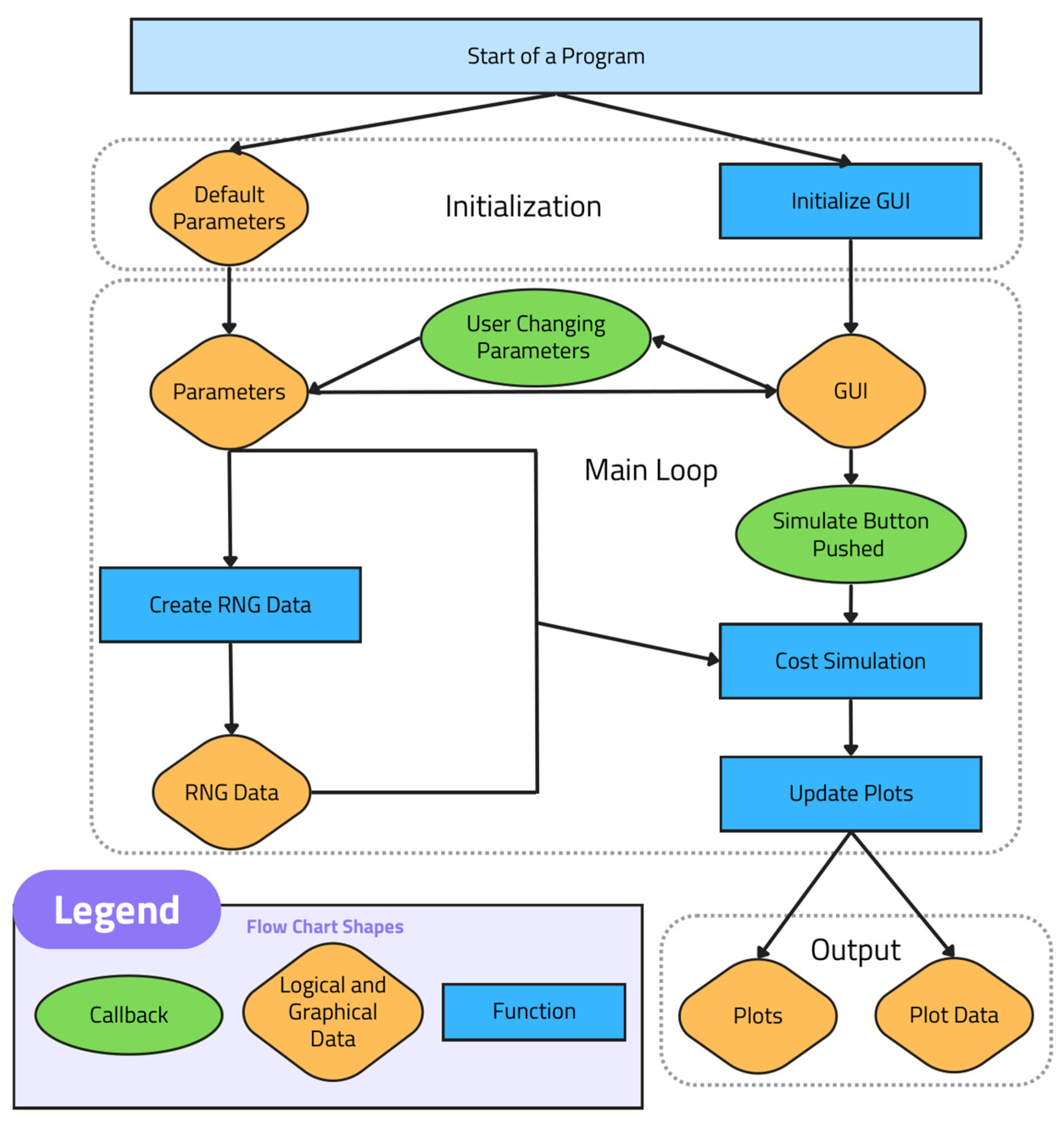
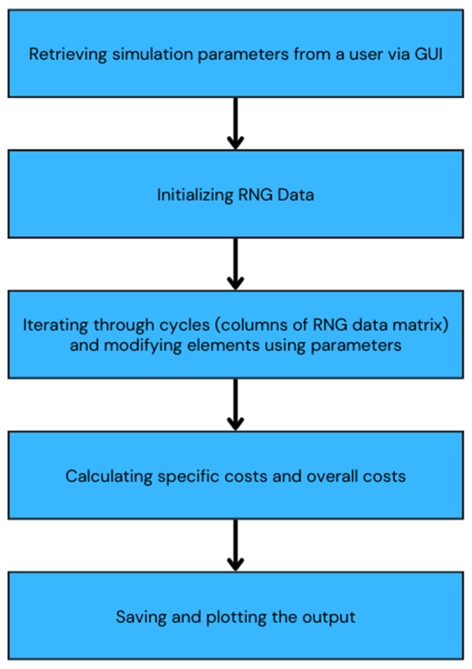
2.3. Simulation of System Maintenance Cost

The authors developed an application for simulating and estimating the costs of system maintenance and repairs in the MATLAB 9.13 (R2022b) environment using additional MATLAB libraries such as the Optimization Toolbox and Statistics Toolbox. Figure 3 displays a flowchart of the program, with layers labeled as Initialization, Main Loop, and Output. The application is versatile and allows for cost analysis of renewable systems by implementing the aforementioned model.

The procedure steps required for cost analysis with the use of the proposed application are presented below:

• First, the user enters data in the presentation layer and the communication layer of the application. Section 3 provides a detailed description of the parameters required to perform the simulation.
  • Determine the number of system reliability states and parameters of each of these states.
  • Define the maintenance and repair strategy and set the repair objectives for a system, i.e., decide whether repair actions are carried out in a given state and, if so, to what state the system is repaired, taking into account the possibility of perfect and imperfect repairs.
  • Determine the cost and the duration of repairs for the system to reach individual reliability states from other, worse states.
  • Determine the remaining necessary parameters for the operation and repair of the system. Such parameters include the operational costs of running and servicing the system in individual reliability states and the costs of inspections.
  • Decide whether emergency repairs are possible and input the related parameters such as delay, additional cost, and trigger conditions.
• The entered data related to the application is stored and managed in the data layer. These data are then processed by the application to estimate costs through a simulation. An illustration of cost simulation function is shown in the flowchart (Figure 4). Further description of the application is provided in Section 3.2 and Section 3.3. Again, for the sake of clarity, we do not include the steps related to emergency repair.
• The cost simulation application allows for the estimation of total costs of system maintenance and repair as well as comparison of different inspection and repair objectives. The results are graphically illustrated in the presentation layer with the possibility of analyzing the cost structure. To standardize the results of simulations, costs are normalized and provided per time unit. The simulation results for a water management system are described in Section 3 and discussed in Section 4.

3. Simulation Model and Its Application to a Water Management System

3.1. Water Management System Reliability States

Reliability states of technical systems are usually divided into two main categories: states of fitness (also referred to as ability/safety/reliability states) and states of unfitness (inability/failure/unreliability states) [60,61,62,63]. States of fitness represent a system’s readiness to process its operational tasks and ability to maintain its functional capabilities [64,65]. States of unfitness represent, in general, a system’s failures, meaning its inability to fulfil its operational characteristics and loss of functional ability, fully or partially [66,67]. The literature also includes a number of examples of intermediate states, illustrating system functionality between states of entire reliability and of total inability. The intermediate states are generally denominated as “Emergency” [61,62,68] or “Under Threat” [69,70,71]. In general, the emergency or under-threat states represent a situation when system operation is disrupted by unintentional events, but the system is partially able to process its operational tasks or incompletely maintain its functional capabilities.

For the purposes of this article, four reliability states of water management systems are determined, reflecting costs generated by the system operating at a certain reliability state (previously described as “state costs”):

• State 1: state of entire ability—representing a situation when the water management system is fully processing its operational tasks at minimal state cost.
• State 2: state of restricted ability—appearing when disruptions of unintentional events interfere with system functionality. The system is still able to process its operational tasks and is fully able to maintain its functional capabilities; however, this state is associated with a rise in operational costs.
• State 3: state of emergency—disruptions within the system result in its restricted ability to process operational tasks; the system’s functional capabilities are also decreased. Simultaneously, state cost is significantly higher.
• State 4: state of total inability—emerging when the system stops operating and is unable to maintain its functional capabilities.

3.2. Application Parameters and Assumptions

In order to simulate operation of the system and calculate its maintenance cost, our application requires the user to provide several parameters. We present them in this section along with assumptions regarding the water management system.

3.2.1. System Parameters and Assumptions

As our optimization problem focuses on determining a maintenance and repair strategy, in a simulation program, we normalize cost-related parameters and obtain total costs per time unit. We include the following parameters in the simulation:

• Inspection Objectives—the objectives of the inspection have to be defined in the case of a multistate system; for each imperfect state of the system, we declare whether it should be repaired to a perfect state, to some improved imperfect state, or not repaired at all; for the water management system, we assume that only perfect repairs (to the state of entire ability) are carried out (perfect repair can also mean replacing a system component with a new one). However, since State 2, of restricted ability, allows the operation of the system, we consider and compare two cases: “always repair” (repair when either of States 2, 3, or 4 is detected) and “repair from State 3” (that is, repair if a state of emergency or system failure is detected, and leave State 2 unrepaired);
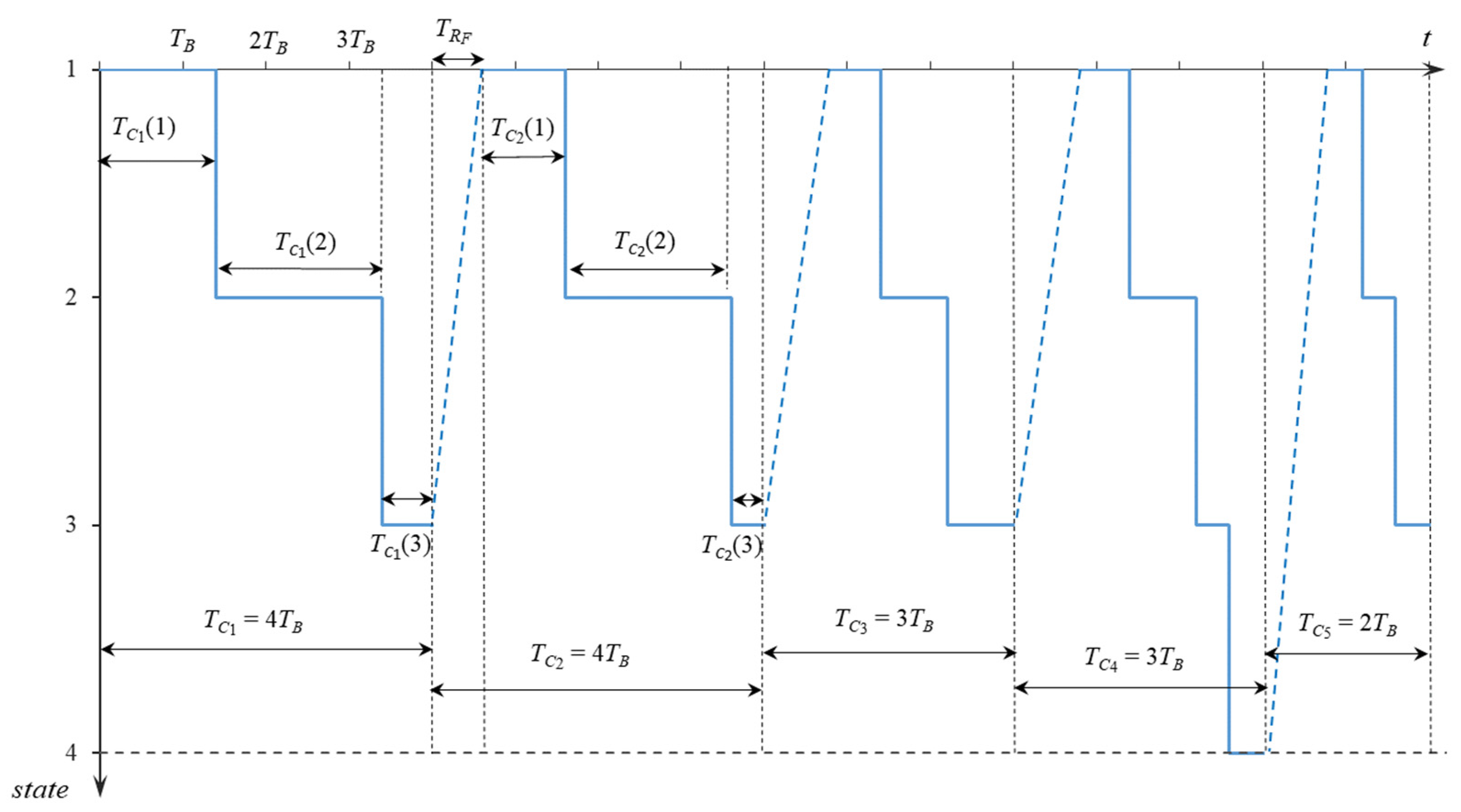
• Emergency Repair Option—additional option of conducting repairs between scheduled inspections at extra cost. In the case study, we assume the emergency crew can be called immediately if the system reaches State 4 (the system operation stops) and no inspection is scheduled within the next 5 days. They arrive 2 days later (assumed delay), carry out the inspection and repair at usual costs, and charge an additional five units of cost for the unplanned repair. We also consider the possibility of calling them in State 3 (assuming that deterioration to the state of threat is self-announced);
• Repair Cost—direct costs related to the repair, such as the cost of repairs or replacement of components/subassemblies and the costs of labor of the servicing crew. For a multistate system, these costs may differ depending on the desired repair effect. For the case study, we assume the perfect repair costs two units of cost from State 2, three units from State 3, and ten units from State 4;
• Repair Time—the time required to perform a given variant of repair during which the system becomes shut down, resulting in additional operational costs. For the case study, we assume that repair from State 4 takes 4 days. As the repair from State 2 and State 3 in the considered system does not require a shutdown, we consider zero to be their Repair Time value;
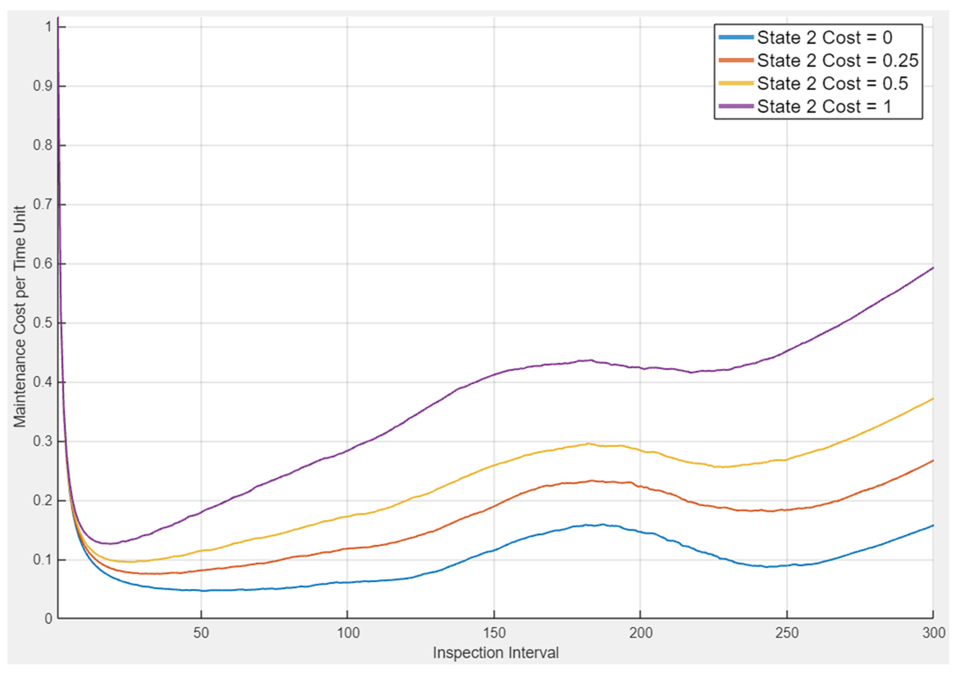
• State Cost—all additional reliability associated costs per time unit; these costs are provided for each reliability state of the system as they are generated by the system operating in that state; apart from regular costs related to operation, it may also include the loss of profit (for example, due to the hydroelectric plant working at reduced efficiency). In the case study, the state cost (daily cost of the system being in imperfect state) is 0.5 of cost unit for State 2, 2 units for State 3, and 10 for State 4;
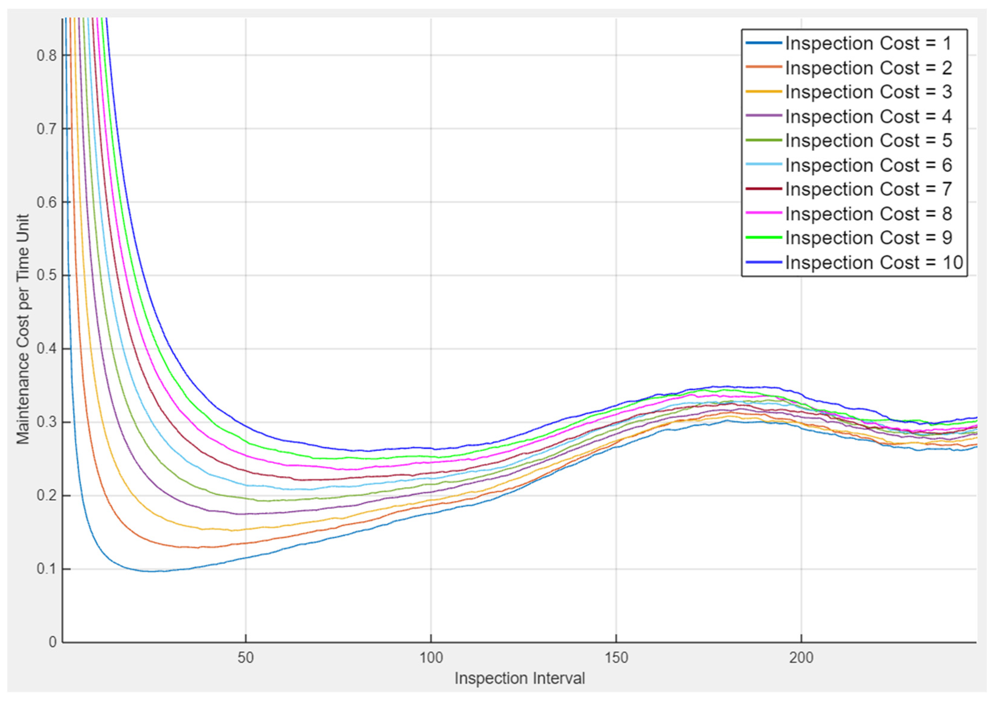
• Inspection Cost—a fixed cost of each inspection performed, regardless of whether it results in performing a repair or not; inspections occur periodically and are called off only when they happen during an ongoing repair. We assume that an inspection either does not require the shutdown of the system or that the time of such shutdown is negligible and, in that case, the cost of the shutdown should be included as a part of the Inspection Cost parameter. For the case study, we assume it equals one unit of cost.

In the version of the computer application presented, we assume that the times of the system being in reliability states or in reliability state subsets follow Weibull distributions with shape and scale parameters provided by a user. The model that is proposed is a general one and can be applied for various system reliability distributions. It is possible to use any other distributions with a slight modification of the code.

We recall that the probability density function of Weibull distribution with scale α and shape β is provided by

$$f_{\alpha ,\beta }\left(x\right)=\left\{\begin{array}{c}\frac{\beta }{\alpha }{\left(\frac{x}{\alpha }\right)}^{\beta -1}{e}^{-{\left(\frac{x}{\alpha }\right)}^{\beta }}, x \ge 0\\ 0, x<0\end{array}\right.,$$

(8)

and the cumulative probability function is

$$F_{\alpha ,\beta }\left(x\right)=1-e^{-{\left(\frac{x}{\alpha }\right)}^{\beta }}.$$

(9)

In the literature, lifetimes of a system and its components often follow such distributions [72,73]. Waghmode and Sahasrabudhe [72] used a stochastic point process to describe the reliability of a repairable system and Weibull distribution to model system lifetime. The approach proposed in [72] is applied to a typical repairable system such as an industrial pump. In [73], Weibull distribution was applied to describe the reliability of multistate components of wind farm infrastructure. Debón et al. [74] applied the Weibull model and analyzed the risk of failure for water supply networks by using Weibull distribution. Liuzzo et al. [38] used the Weibull distribution to describe water demand in order to provide reliability analysis of a rainwater harvesting system. Kossieris and Makropoulos [75] applied the Weibull distribution to model residential water demand for efficient water system management. In this paper, we use the Weibull distribution to describe the reliability of a water management system; more precisely, to model the times of a system being in reliability state subsets.

In the simulation program, for the assumed Weibull distribution, we have to provide its parameters, i.e., the Weibull shape and scale parameters. These parameters are provided for the times of the system being in reliability states in the Gradual Degradation Mode and for the times of the system being in reliability state subsets in the Shock Degradation Mode. For a water management system, we consider the possibility of unexpected system failure from any reliability state; hence, we refer to the second of the above cases.

We consider a water management system as a four-state system with reliability states defined in Section 3.1. Consequently, the cumulative probability functions corresponding to a system’s lifetimes in reliability state subsets are provided. The values of scale parameters are estimated per year. For the time of a system’s being in the state of entire ability $T_{sub}\left(\left\{1\right\}\right)$, i.e., State 1, it takes the following form:

$$F\left(t, T_{sub}\left(\left\{1\right\}\right)\right)=1-e^{-{\left(\frac{t}{0.4597}\right)}^4}.$$

(10)

The cumulative probability function for time $T_{sub}\left(\left\{\mathrm{1,2}\right\}\right)$of a system being in a state subset {1, 2}, i.e., in a state of entire or restricted ability, is

$$F\left(t, T_{sub}\left(\left\{\mathrm{1,2}\right\}\right)\right)=1-e^{-{\left(\frac{t}{1.1033}\right)}^4}.$$

(11)

Finally, the cumulative probability function for system lifetime $T_{sub}\left(\{\mathrm{1,2},3\}\right)$, corresponding to the time until a system’s total loss of function, is

$$F\left(t, T_{sub}\left(\{\mathrm{1,2},3\}\right)\right)=1-e^{-{\left(\frac{t}{1.7206}\right)}^3}.$$

(12)

3.2.2. Simulation Parameters

The application requires that the following parameters are set before the simulation is run:

• Production Cycles—this parameter determines the supposed duration of the run of the simulation. In general, the higher the number of production cycles, the more stable the results of the simulation. Each production cycle ends exactly at the beginning of a new repair, which happens at the start of the next cycle. If the system reaches the state of total loss of function and the inspection objective for that state is “do not repair”, it cannot be repaired ever again. In that unordinary case, the production cycle is terminated at the time of the nearest inspection.
• Min/Max Interval—these values identify the minimal/maximal inspection interval considered in the simulation.
• Step—the fixed difference between two consecutive inspection intervals considered in the simulation. For example, if our intention is to generate the plot for intervals 10, 15, 20, …, 100, we set Min Interval = 10, Max Interval = 100, and Step = 5.
• Run … Times—if this box is checked, the simulation runs the chosen number of times. Then, in the Cost Plot tab, three curves are displayed, depicting the maximal, minimal, and average values obtained for each inspection interval. In the current version of the application, this checkbox does not alter the way other plots are generated.
• Hold The Data—if the box is checked, a new Cost Plot is added on top of previously drawn plots without removing them. This is useful for comparisons.

3.3. Application Description and Results

Upon the launch of the application, a GUI is initialized and default parameters are loaded. The Cost Simulation function is then executed using these parameters, and initial plots are drawn. From this point on, the user can change the parameters in the GUI and execute the simulation by clicking the “Simulate” button. The plots are automatically drawn after the calculations are completed. The flowchart of cost simulation, illustrating the application’s operation and individual stages of data processing, is presented in Figure 4.

The cost simulation application we created allows the analysis of the structure of total cost by distinguishing direct cost of repairs, cost of all inspections, and operational cost. State Structure Plot allows the comparison of the percentage of a system being in certain reliability states and in repair. Since the overall time of the system running within the simulation depends both on the initial parameters and on the random values sampled from the Weibull distributions, Total Cost by itself is not a good variable when it comes to further analysis. It requires normalization; we divide it by the total time of the system running in order to estimate the cost per single unit of time.

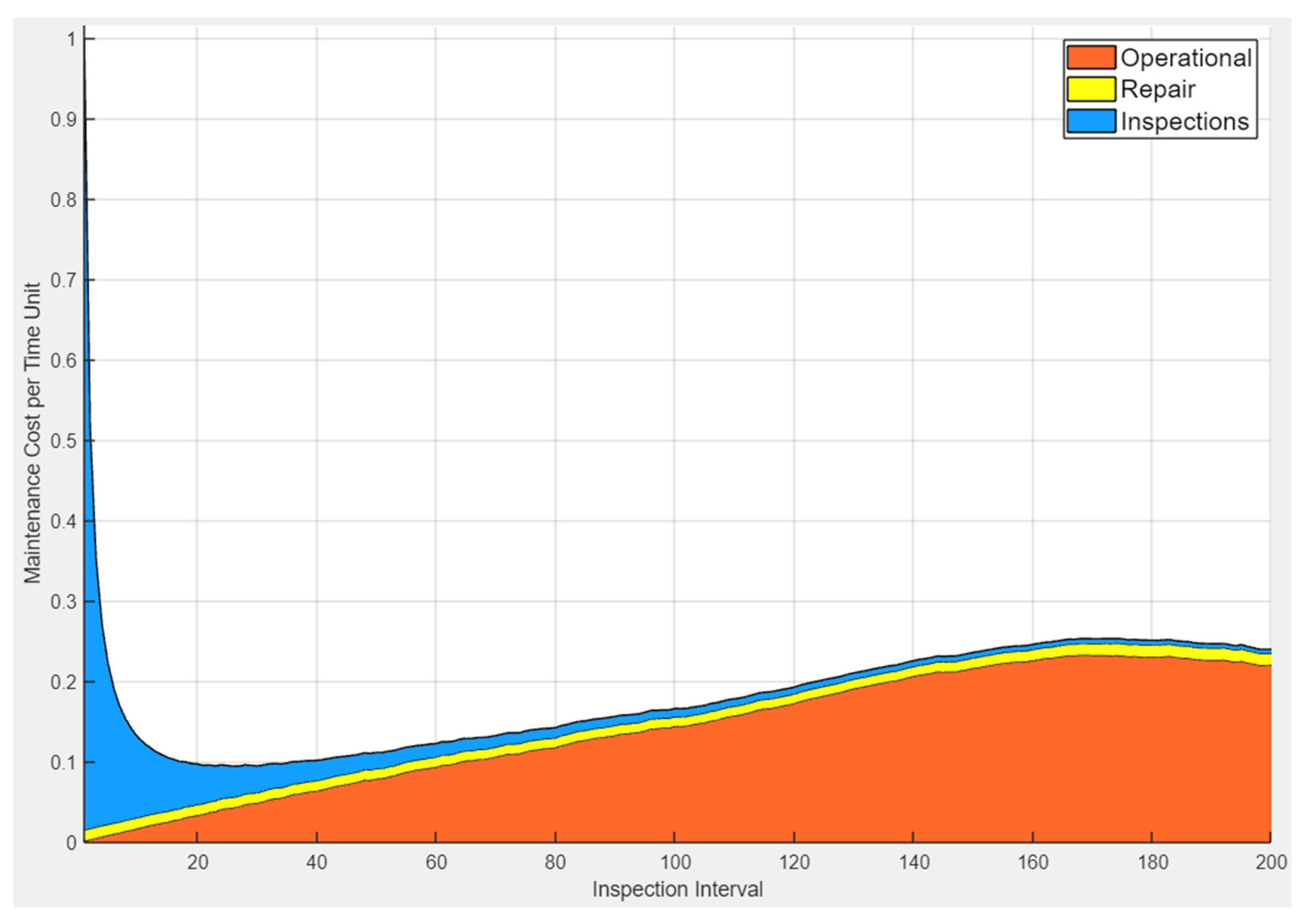
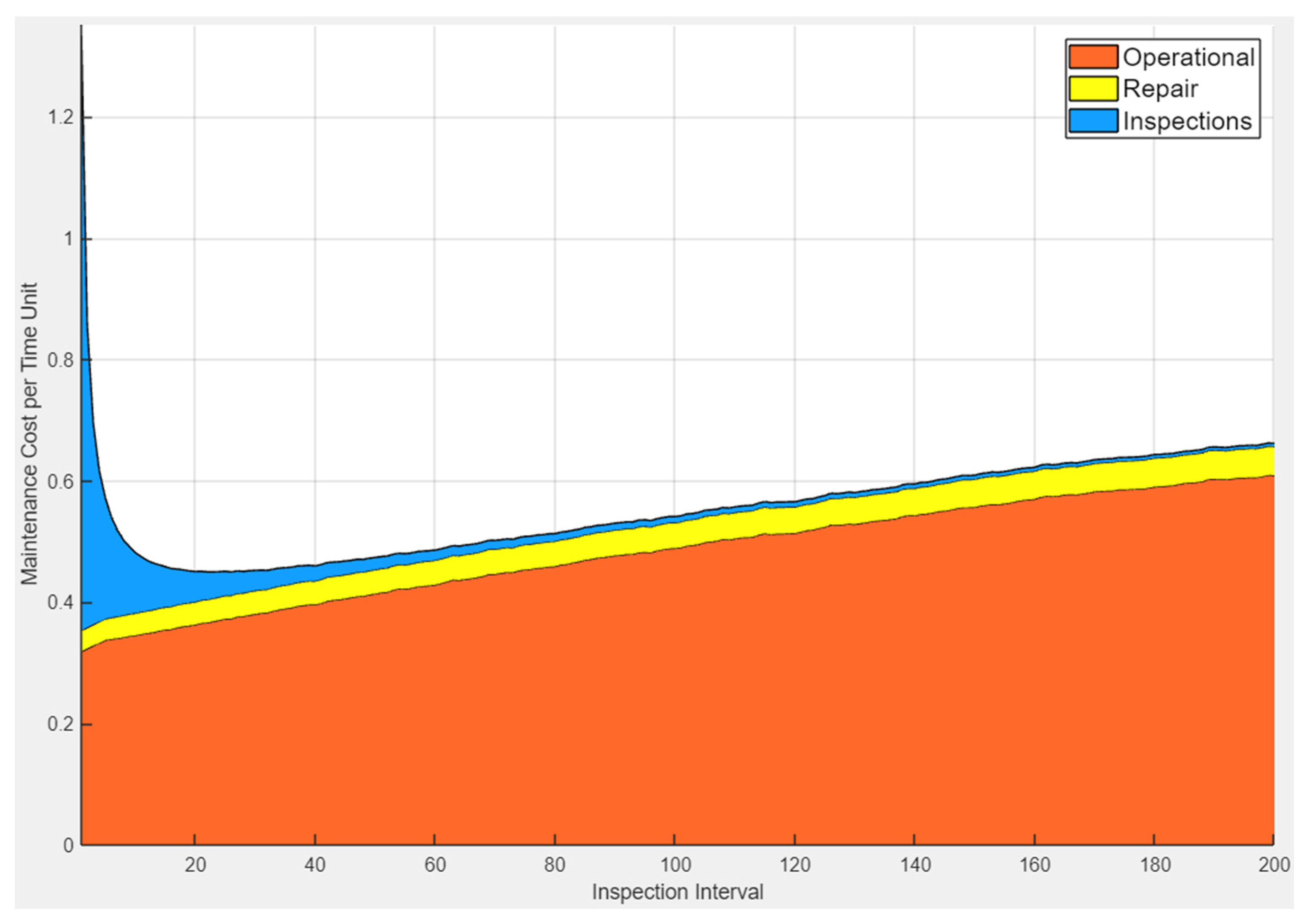
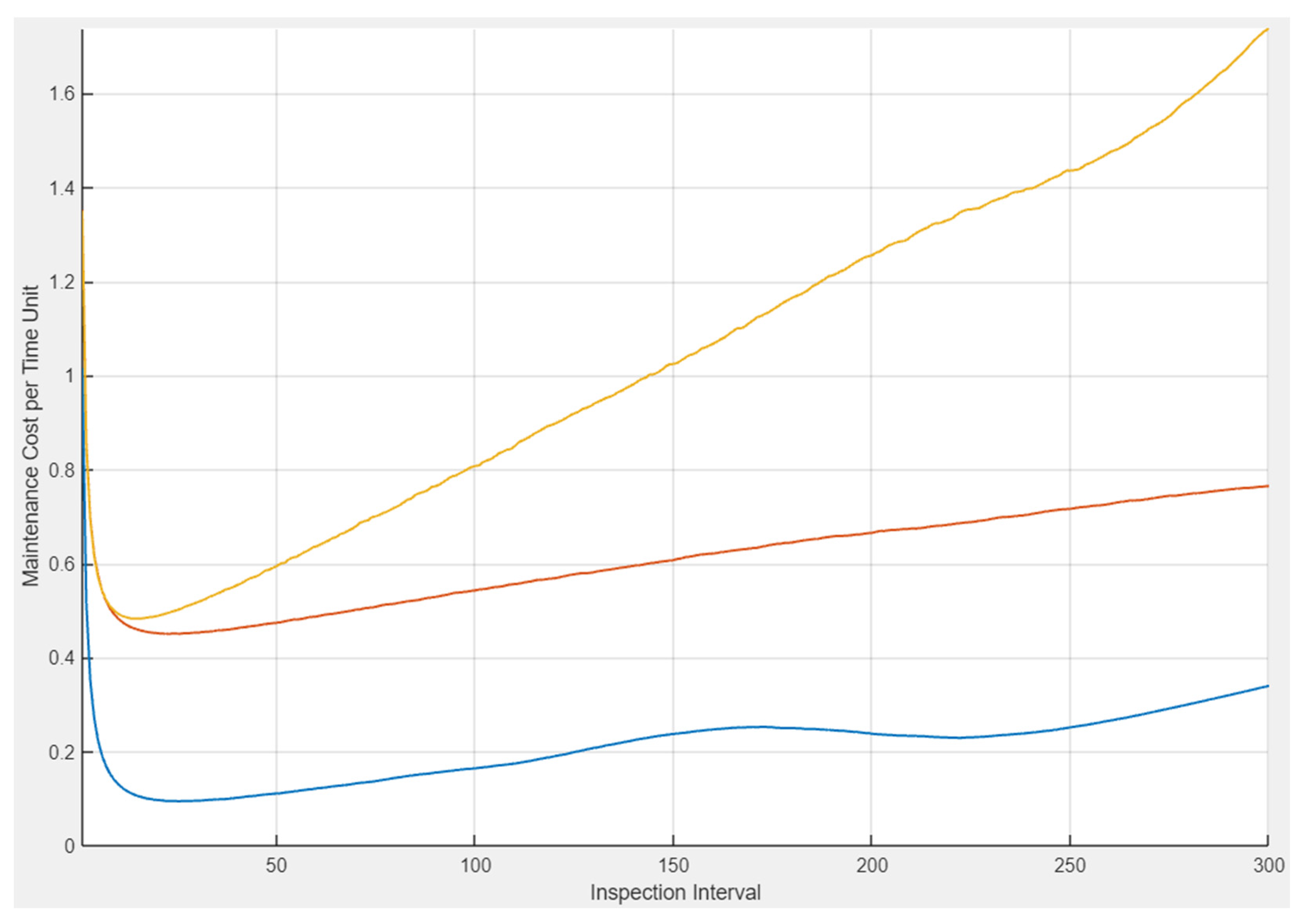
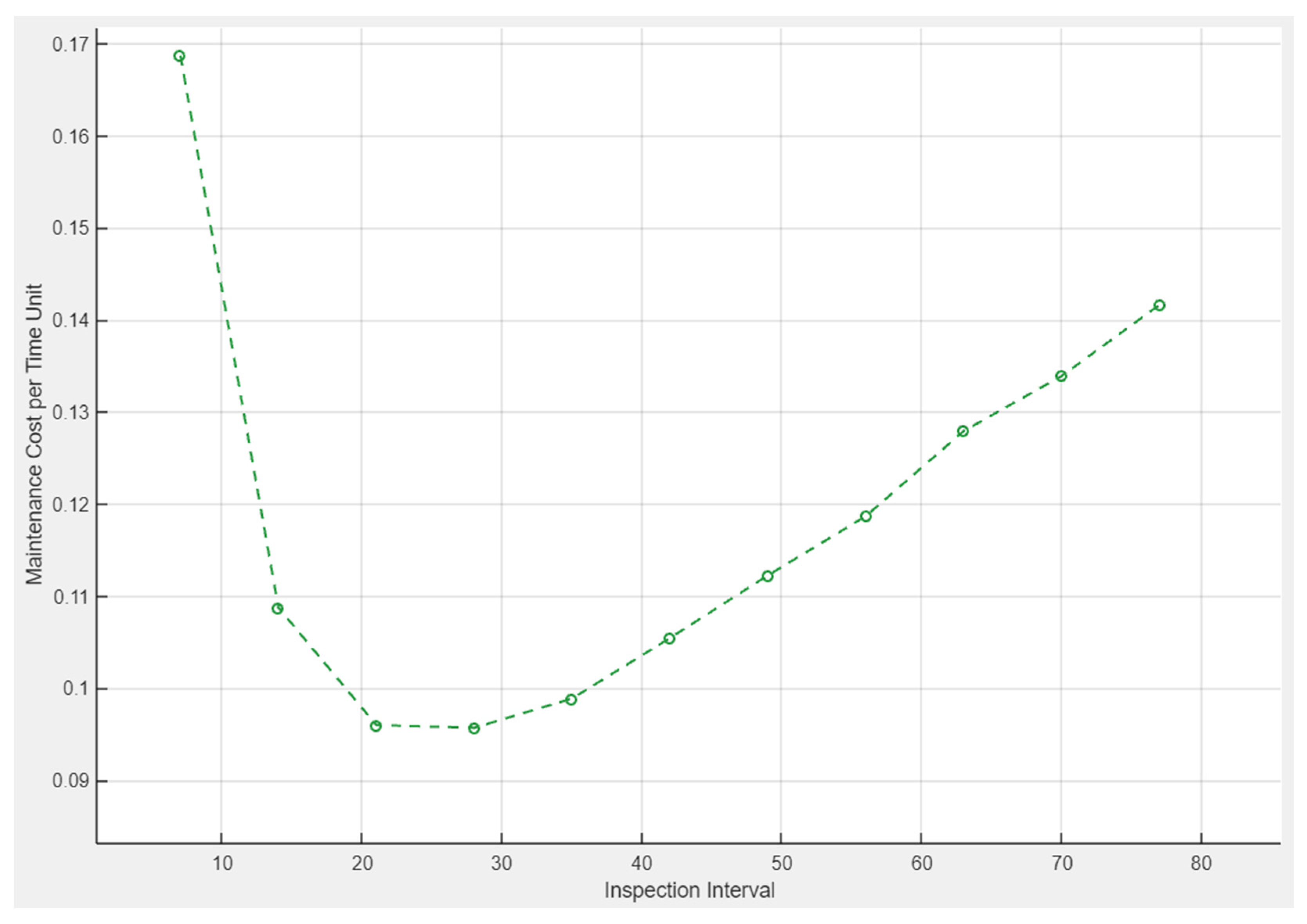
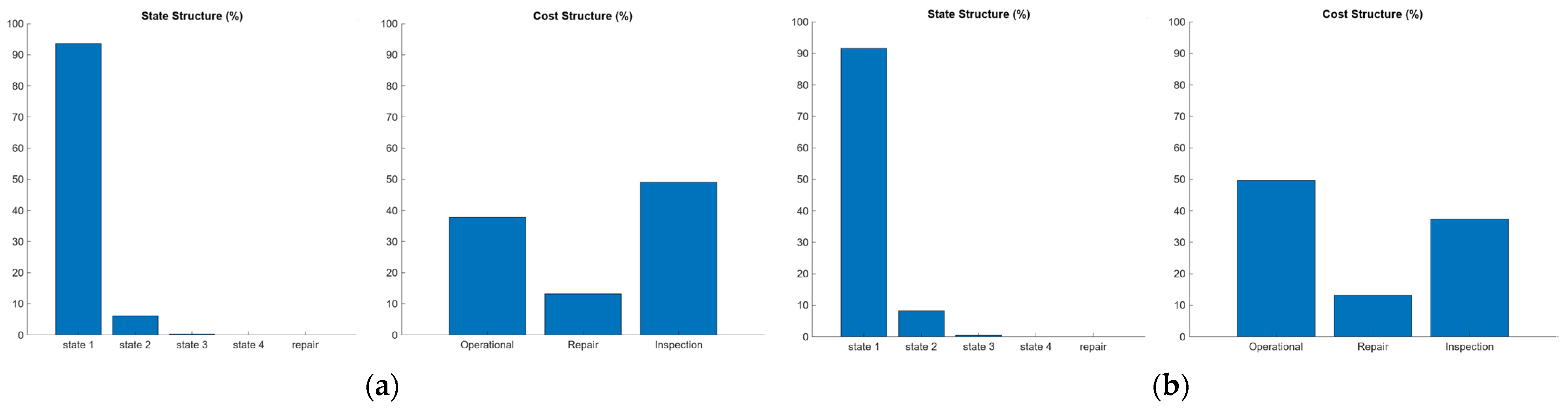
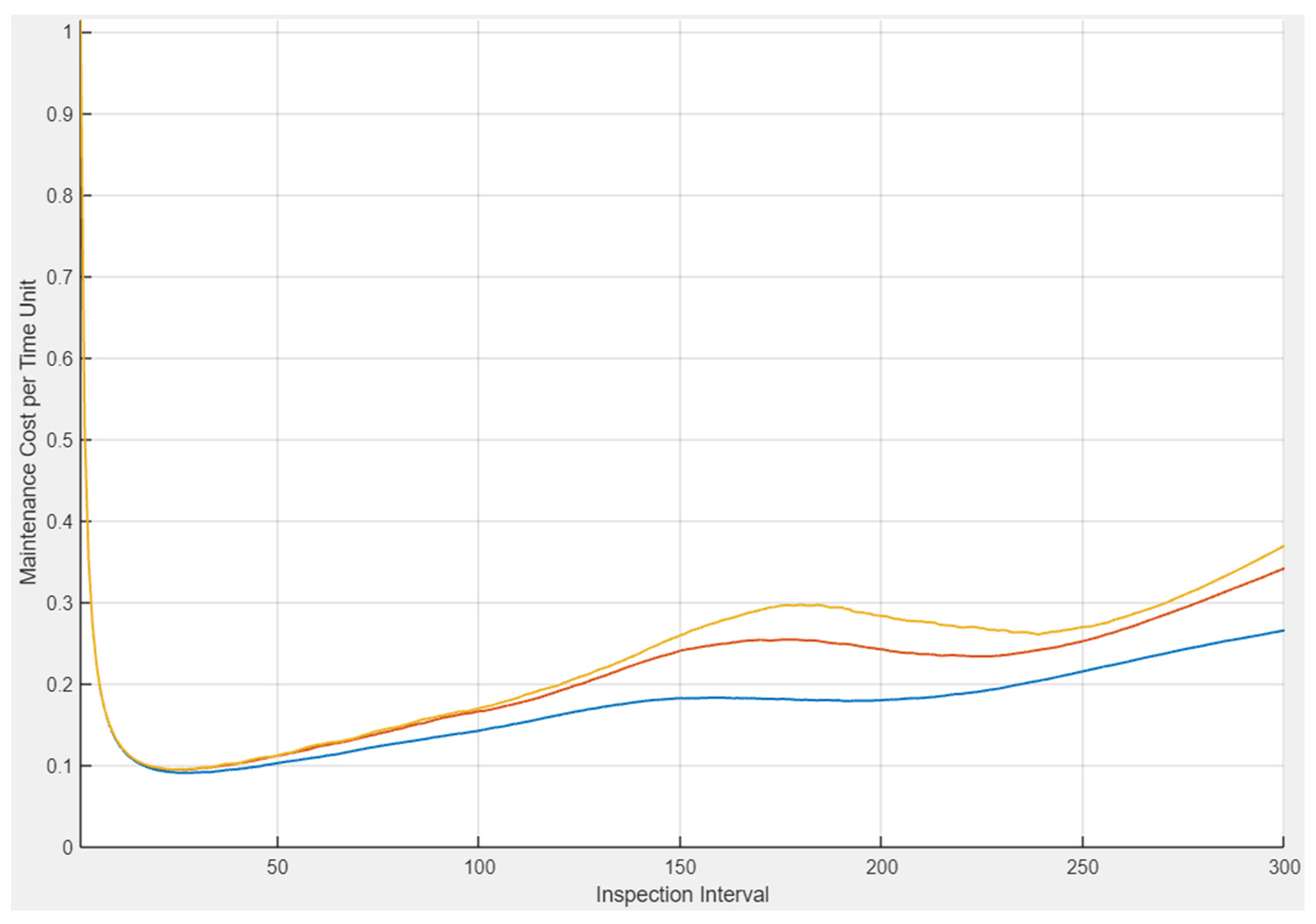
3.4. Case Study Results

This subsection presents the analysis of the operation and the maintenance cost of a water management system, obtained from a simulation program created in the MATLAB environment. The application is described in Section 2.3 and Section 3.3 of this paper. The analysis is conducted under assumptions provided in Section 3.2, according to the methodology presented in Section 2. As a result of simulation, we obtain the total operation and maintenance costs normalized per unit of time, calculated for different values of inspection intervals T_B. Cost simulation by the application allows for the analysis of total cost structure and indicates the optimal value of inspection interval that minimizes total cost under the assumed maintenance strategy. Moreover, the simulation application allows the comparison of results for various parameters and inspection objectives, reinforcing the decision-making process of choosing the optimal maintenance strategy.

Figure 5 and Figure 6 show operation and maintenance cost of the system under a maintenance policy in line with the assumptions provided in Section 3.2.1. Figure 5 refers to the case of conducting repairs if the system, at the moment of inspection, is in State 2 (restricted ability) or worse. This strategy is hereinafter referred to as the “always repair” policy. Figure 6 presents results in the case of conducting repairs if the system is in State 3 or State 4, and we hereafter refer to this policy as “repair from State 3”. In both cases, we assume the possibility of conducting repairs between scheduled inspections at extra cost (referred as “emergency repair”) in the case that the system stops operating.

Figure 5 and Figure 6 additionally show the structure of total operation and maintenance costs, indicating the share of individual cost types, i.e., operational (state costs), repair (with repair associated costs), and inspection costs.

As expected, both in Figure 5 and Figure 6, it is apparent that when inspections happen too frequently, most of them encounter the system in State 1, and these unnecessary inspections generate high costs. On the other hand, when too much time elapses between inspections, the system spends more time in deteriorated states, generating higher operational costs. The inspection interval for which the minimal cost is reached equals 25 days for “always repair” and 23 days for “repair from State 3”. Further graphical comparison of these cases is presented in Figure 7.

The blue plot in Figure 7 highlights the importance of the early recognition of slight damages. For any particular inspection interval, the “always repair” strategy generates less costs than “repair from State 3”. Therefore, as long as it is feasible, the former is a more beneficial strategy for the system’s maintenance. With an optimal inspection interval of approximately 25 days, we achieve maintenance cost reduction of around four times compared to the scenario without early damage recognition. Due to the emergency team’s response time being relatively low, it is evident that an emergency repair strategy is crucial for minimizing costs for longer inspection intervals, whereas its influence on maintenance cost or optimal maintenance interval is of less importance.

For practical reasons, it is often convenient for periodic inspections to always be scheduled on the same weekday. In that case, we consider only inspection intervals of 7, 14, 21 days, etc. (Figure 8). Results presented in Figure 8 refer to the maintenance strategy named “always repair”, without the emergency repair option.

As can be seen, the daily cost reaches the minimum of circa 0.95 both for the inspection interval of 21 days (every 3 weeks) and 28 days (every 4 weeks). In order to make the decision on which option is preferable, it is convenient to analyze the state and cost structure in each of these cases.

In the structural plots from Figure 9, we observe a decrease in inspection costs and an increase in the operational cost contribution to the overall cost structure when changing the inspection interval from 21 days to 28 days. There is also a slight increase in the participation of State 3, but the change in State 4 participation is negligible. In this example, the choice between either of the two minima does not affect the overall state structure (and system reliability). However, the differences in cost structure are more evident, helping the company to decide which interval to pick depending on its priorities.

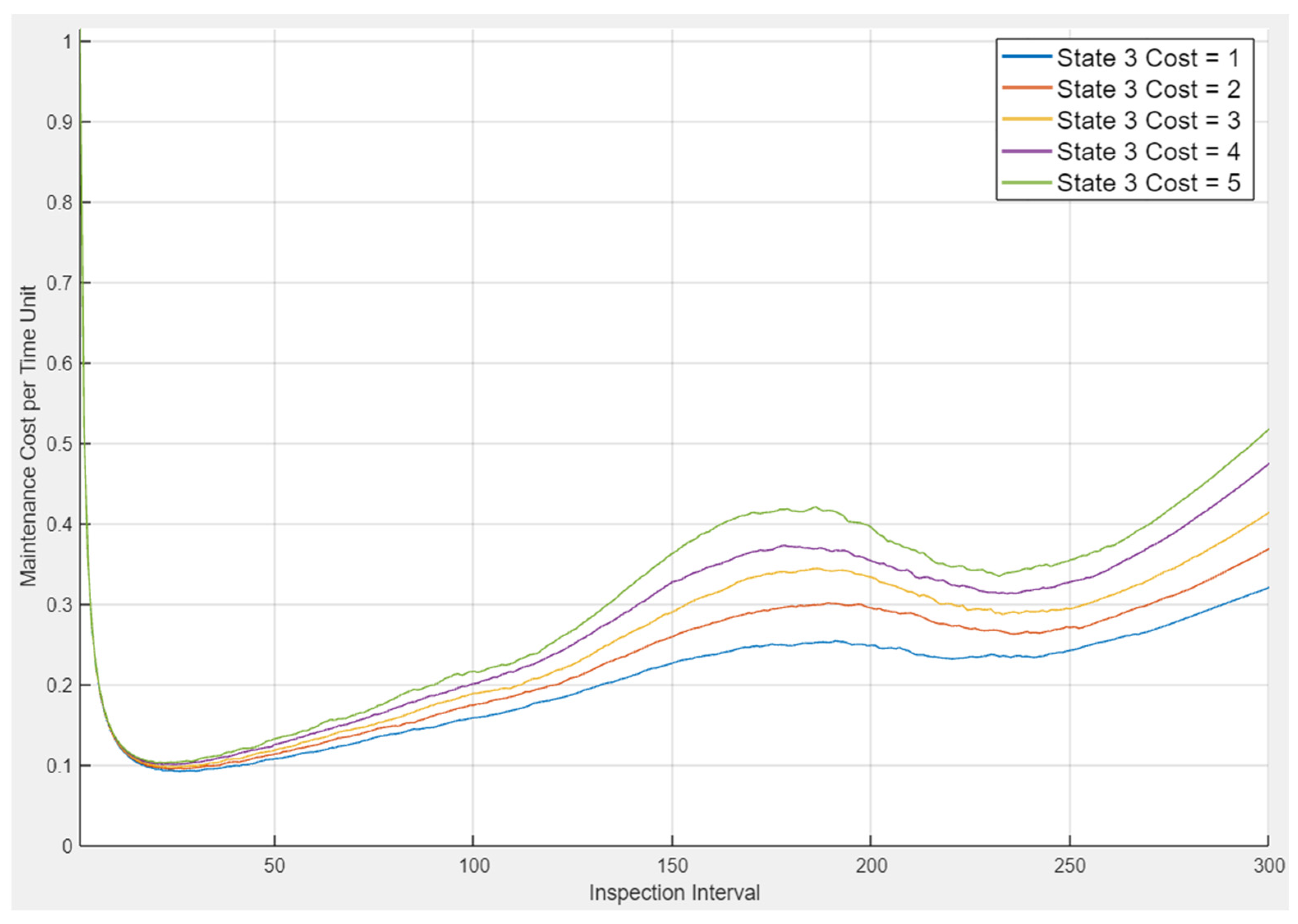
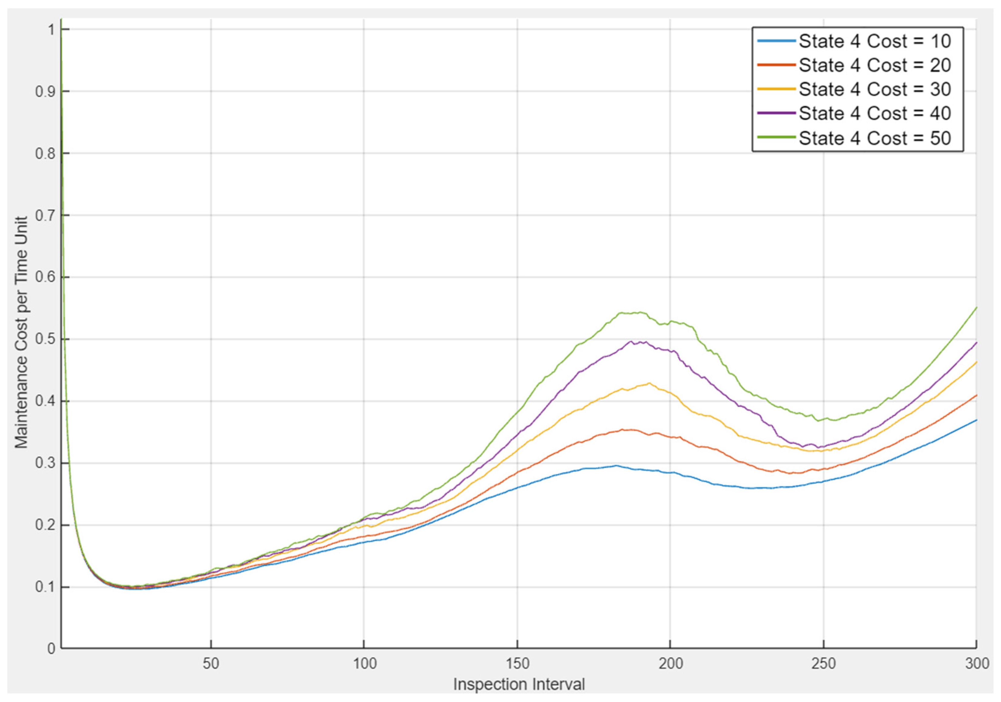
4. Sensitivity Analysis of Cost Parameters and Discussion of Maintenance Strategies

Another aspect that can be adjusted in order to optimize maintenance cost is the set of conditions under which the emergency crew would be called. According to Figure 10, it is generally better to call them as soon as the system reaches State 3 instead of limiting their role to repairing from State 4, that of total loss of function. However, the differences are not very large, proving the effectiveness of the “always repair” policy by itself. In particular, for small inspection intervals, the differences are almost unnoticeable (the frequent inspections are sufficient to keep the system in good condition, making emergency repairs very occasional).

In this plot, we observe the impact of emergency repair conditions on maintenance cost. This influence becomes apparent as the inspection interval length increases, and the most significant difference is observed between emergency actions taken for State 3 and State 4. When the inspection intervals range from 1 to 110, the difference between emergency actions in State 4 and no emergency repairs is negligible. If the emergency team is not readily available, it is advisable to schedule inspections within this mentioned interval range to mitigate potential risks.

The aim of the conducted study is to analyze the results of the total costs for various system maintenance and repair strategies in order to select the best cost–benefit option.

Table 1. Total maintenance costs under “always repair” policy without emergency repair option, estimated per year and referring to a single inspection cost as a unit.

Inspection Interval	Average Yearly Costs (Structure)			Total Yearly Costs
	Operational	Repair	Inspection
10	6.54 (14%)	4.86 (10%)	36.70 (76%)	48.09
15	9.68 (25%)	4.82 (12%)	24.39 (63%)	38.89
20	12.92 (36%)	4.70 (13%)	18.26 (51%)	35.88
25 1	15.67 (45%)	4.69 (13%)	14.63 (42%)	34.99
30	18.89 (53%)	4.64 (13%)	12.17 (34%)	35.70
35	21.94 (59%)	4.54 (12%)	10.45 (28%)	36.93
40	24.65 (64%)	4.52 (12%)	9.16 (24%)	38.34

Note: ¹ optimal value of inspection interval.

presents the results of average yearly costs in the case of an “always repair” policy, assuming that repairs or preventive and corrective actions are carried out only during scheduled inspections without an emergency repair option (referred further as “no emergency opt.”). Total costs, presented in Table 1 and

Table 2. Total maintenance costs under “always repair” policy without emergency repair and with emergency repair option in State 3, estimated per year and referring to a single inspection cost as a unit.

Inspection Interval	Total Yearly Costs		Possible Savings
	“No Emergency Opt.”	“Emergency in State 3”
10	48.09	47.66	0.44 (0.9%)
15	38.89	38.15	0.74 (1.9%)
20	35.88	34.75	1.13 (3.2%)
25	34.99 1	33.55	1.44 (4.1%)
30	35.70	33.35 1	2.35 (6.6%)
35	36.93	33.99	2.94 (8.0%)
40	38.34	35.18	3.16 (8.2%)

Note: ¹ minimal total cost for optimal inspection interval.

, are estimated by using a single inspection cost as a unit. In addition to total repair and maintenance costs, Table 1 illustrates cost structure by separating operational costs related to system exploitation, costs related to the repairs carried out, and inspection costs. Additionally, total cost components (operational, repair, and inspection costs) are provided as a percentage of total yearly costs.

Table 2 compares the total maintenance and repair costs estimated per year in the case of an “always repair” system policy assuming “no emergency opt.”, provided in Table 1, to the results with an emergency repair option in State 3 (referred as “emergency in State 3”).

In further analysis of total system maintenance costs, we consider the “always repair” strategy without an emergency repair option to analyze the sensitivity of results depending on other cost parameters.

Figure 11 features 10 plots depicting system maintenance cost for inspection ranging from 1 to 10 units. System reliability parameters and other cost components do not change. It can be observed that the differences in total costs are significant with regard to frequent inspections. When the intervals between inspections are longer, the differences decrease because of the alternative structure of costs and lower contribution of inspection costs in the total exploitation costs of the system.

In the case of small water structures, the inspection cost can become significant compared to potential daily failure costs or costs associated with reduced efficiency. In such cases, it becomes apparent that the optimal inspection interval increases rapidly for inspection costs ranging from 1 to 5. As the inspection cost increases further, the plots become flatter near the minima. In such a case, we gain more flexibility in choosing an inspection interval without changing the overall maintenance cost.

Table 3. Optimal inspection intervals, minimizing total maintenance costs, for inspection cost ranging from 1 to 10 units.

Inspection Cost 1	Optimal Inspection Interval (in Days)
1	25
2	37
3	46
4	49
5	56
6	67
7	65
8	77
9	84
10	83

Note: ¹ Inspection Cost is expressed in fixed cost unit.

indicates the changes in the optimal length of interval between inspections, minimizing total exploitation and maintenance costs in relation to the cost of a single inspection.

Figure 12 depicts the impact of various operational costs related to the state of restricted ability on the total maintenance cost. When the cost of State 2 is equal to zero, we can consider entering this state as the activation of an early warning system with no influence on the overall system output. It is evident that as the costs generated by State 2 increase, maintenance cost increases and the optimal inspection interval decreases rapidly.

The sensitivity analysis, due to differences in operational costs related to exploitation of the system in State 3, is shown in Figure 13. The costs are expressed by certain units for one day of exploitation, and thus, their share in total exploitation and repair costs of the system depends also on the time of the system staying in this state. It can be noted that the differences in the total costs are low at relatively short inspection intervals. The optimal values of these intervals, with exploitation costs in State 3 increasing from one to five per day, slowly decrease from 27 days to 23 days. However, overall cost remains similar for these five cases. This follows from the fact that frequent inspections result in rapid detection of any fluctuations in the system, and consequently the time of the system staying in State 3 is short. The analysis of sensitivity of the total system maintenance costs, associated with increase in costs related to the system being in State 4, is very similar (Figure 14).

5. Conclusions

One of intended objectives of water management systems, including water supply and water distribution systems, which are critical municipal infrastructures, is ensuring communities and industries receive an uninterrupted supply of safe and clean (within certain parameters) water, while taking into account its ever-increasing demand. In this context, the planning of maintenance and repair of the system leading to its undisrupted and possibly low-cost performance is a crucial and tangible issue. Concerning the cost–benefit analysis of such systems, it is important to minimize total cost while simultaneously ensuring the system’s uninterrupted operation and maintenance of its functional capabilities. The proposed model and software, constructed on this basis, allows to the conduction of analysis of the maintenance and repair costs of systems for various repair objectives and inspection intervals. As a result, we can determine a maintenance and repair strategy that minimize the total cost. Moreover, the proposed multistate approach to degradation description allows to the setting of the rules regarding conducting repairs, depending on the system condition, corresponding to a certain reliability state. In this way, we can look for the most cost-effective strategy for the system’s upkeep while satisfying safety requirements corresponding to the system’s reliability level. Estimated cost does not have to be interpreted as purely financial, as one can also adjust the cost parameters to reflect incalculable risks and consequences. The structure of maintenance costs and reliability states allows the monitoring of whether a given strategy guarantees fulfilling additional requirements. Therefore, the simulation application can support the decision-making process of choosing a maintenance strategy for water management systems.

The assumption of the analysis and optimization of the system maintenance cost proposed in the manuscript considers the system as a single unit and does not take into account its reliability structure. Our future research will also take into account the system’s reliability structure and the reliability of its components considering eventual dependencies among them or subsystems that the system is built of. In this context, we plan to conduct deep analysis of systems related to water supply for societies and water treatment systems, both in terms of optimization of their exploitation and repairs, and analysis of their reliability and availability, taking into account their structure. One of the system types that can be analyzed and optimized in this way is membrane-based point-of-use water treatment systems. This has become a revolutionary technique in water treatment technologies and is widely analyzed in [76].

References

1. Cole, J.; Sharvelle, S.; Grigg, N.; Pivo, G.; Haukaas, J. Collaborative, Risk-Informed, Triple Bottom Line, Multi-Criteria Decision Analysis Planning Framework for Integrated Urban Water Management. Water 2018, 10, 1722. [Google Scholar] [CrossRef]
2. Larsen, T.; Gujer, W. The concept of sustainable urban water management. Water Sci. Technol. 1997, 35, 3–10. [Google Scholar] [CrossRef]
3. Masia, O.A.; Erasmus, L.D. Smart metering implementation for enabling Water Conservation and water demand management: An investigation in Gauteng, South Africa. In Proceedings of the 2013 Africon, Pointe aux Piments, Mauritius, 9–12 September 2013. [Google Scholar] [CrossRef]
4. Stewart, R.A.; Willis, R.; Giurco, D.; Panuwatwanich, K.; Capati, G. We-based knowledge management system: Linking smart metering to the future of urban water planning. Aust. Plan. 2010, 47, 66–74. [Google Scholar] [CrossRef]
5. Marques, J.; Cunha, M.; Savi´c, D.A. Multi-objective optimization of water distribution systems based on a real options approach. Environ. Model. Softw. 2015, 63, 1–13. [Google Scholar] [CrossRef]
6. Bithas, K. The sustainable residential water use: Sustainability, efficiency and social equity. The European experience. Ecol. Econ. 2008, 68, 221–229. [Google Scholar] [CrossRef]
7. Esmail, B.A.; Suleiman, L. Analyzing Evidence of Sustainable Urban Water Management Systems: A Review through the Lenses of Sociotechnical Transitions. Sustainability 2020, 12, 4481. [Google Scholar] [CrossRef]
8. Marlow, D.R.; Moglia, M.; Cook, S.; Beale, D.J. Towards sustainable urban water management: A critical reassessment. Water Res. 2013, 47, 7150–7161. [Google Scholar] [CrossRef]
9. Cettner, A.; Söderholm, K.; Viklander, M. An adaptive stormwater culture? Historical perspectives on the status of stormwater within the Swedish Urban Water System. J. Urban Technol. 2012, 19, 25–40. [Google Scholar] [CrossRef]
10. Quezada, G.; Walton, A.; Sharma, A. Risks and tensions in water industry innovation: Understanding adoption of decentralised water systems from a socio-technical transitions perspective. J. Clean. Prod. 2016, 113, 263–273. [Google Scholar] [CrossRef]
11. Bagirov, A.M.; Barton, A.F.; Mala-Jetmarova, H.; Al Nuaimat, A.; Ahmed, S.T.; Sultanova, N.; Yearwood, J. An algorithm for minimization of pumping costs in water distribution systems using a novel approach to pump scheduling. Math. Comput. Model. 2013, 57, 873–886. [Google Scholar] [CrossRef]
12. Van Dijk, M.; van Vuuren, S.J.; van Zyl, J.E. Optimising water distribution systems using a weighted penalty in a genetic algorithm. Water SA 2008, 34, 537–548. [Google Scholar] [CrossRef]
13. Lopez-Ibanez, M.; Devi Prasad, T.; Paechter, B. Ant colony optimization for optimal control of pumps in water distribution networks. J. Water Resour. Plan. Manag. 2008, 134, 337–346. [Google Scholar] [CrossRef]
14. van Zyl, J.E.; Savic, D.A.; Walters, G.A. Operational optimization of water distribution systems using a hybrid genetic algorithm. J. Water Resour. Plan. Manag. 2004, 130, 160–170. [Google Scholar] [CrossRef]
15. Pamidimukkala, A.; Kermanshachi, S.; Adepu, N.; Safapour, E. Resilience in Water Infrastructures: A Review of Challenges and Adoption Strategies. Sustainability 2021, 13, 12986. [Google Scholar] [CrossRef]
16. Mwendera, E.J.; Hazelton, D.; Nkhuwa, D.; Robinson, P.; Tjijenda, K.; Chavula, G. Overcoming constraints to the implementation of water demand management in southern Africa. Phys. Chem. Earth 2003, 28, 761–778. [Google Scholar] [CrossRef]
17. Gupta, A.D.; Pandey, P.; Feijóo, A.; Yaseen, Z.M.; Bokde, N.D. Smart Water Technology for Efficient Water Resource Management: A Review. Energies 2020, 13, 6268. [Google Scholar] [CrossRef]
18. Xiang, N.; Sha, J.; Yan, J.; Xu, F. Dynamic Modeling and Simulation of Water Environment Management with a Focus on Water Recycling. Water 2014, 6, 17–31. [Google Scholar] [CrossRef]
19. Xuan, X.J.; Xu, H. Use of Reclaimed Water in China: Management issues and strategies. Manag. Sci. Eng. 2009, 3, 17–25. [Google Scholar] [CrossRef]
20. Angelakis, A.N.; Bonoux, L.; Lazarova, V. Challenges and prospective for water recycling and reuse in EU countries. Water Sci. Technol. 2003, 3, 59–68. [Google Scholar] [CrossRef]
21. Asano, T.; Cotruvo, J.A. Groundwater recharge with reclaimed municipal wastewater: Health and regulatory considerations. Water Res. 2004, 38, 1941–1951. [Google Scholar] [CrossRef]
22. Global Water Partnership–Technical Advisory Committee (GWP-TAC). Integrated Water Resources Management; Background Paper No. 4; Global Water Partnership, Technical Advisory Committee: Stockholm, Sweden, 2000. [Google Scholar]
23. Beck, M.B. Water quality modeling: A review of the analysis of uncertainty. Water Resour. Res. 1987, 23, 1393–1442. [Google Scholar] [CrossRef]
24. Young, P. Data-based mechanistic modelling of environmental, ecological, economic and engineering systems. Environ. Model. Softw. 1998, 13, 105–122. [Google Scholar] [CrossRef]
25. D’Ambrosio, C.; Lodi, A.; Wiese, S.; Bragalli, C. Mathematical programming techniques in water network optimization. Eur. J. Oper. Res. 2015, 243, 774–788. [Google Scholar] [CrossRef]
26. Dennison, F.J.; Azapagic, A.; Clift, R.; Colbourne, J.S. Life cycle assessment: Comparing strategic options for the mains infrastructure d part I. Water Sci. Technol. 1999, 39, 315–319. [Google Scholar] [CrossRef]
27. Cohen, D.; Shamir, U.; Sinai, G. Optimal operation of multi-quality water supply systems-II: The Q-H model. Eng. Optim. 2000, 32, 687–720. [Google Scholar] [CrossRef]
28. Ostfeld, A.; Shamir, U. Optimal operation of multiquality networks. I: Steady-state conditions. J. Water Resour. Plan. Manag. 1993, 119, 645–662. [Google Scholar] [CrossRef]
29. Ostfeld, A.; Shamir, U. Optimal operation of multiquality networks. II: Unsteady conditions. J. Water Resour. Plan. Manag. 1993, 119, 663–684. [Google Scholar] [CrossRef]
30. Deak, J.; Bucht, E. Planning for climate change: The role of indigenous blue infrastructure, with a case study in Sweden. Town Plan. Rev. 2011, 82, 669–685. [Google Scholar] [CrossRef]
31. Cettner, A.; Ashley, R.; Viklander, M.; Nilsson, K. Stormwater management and urban planning: Lessons from 40 years of innovation. J. Environ. Plan. Manag. 2013, 56, 786–801. [Google Scholar] [CrossRef]
32. Echols, S. Artful rainwater design in the urban landscape. J. Green Build. 2007, 2, 101–122. [Google Scholar] [CrossRef]
33. Brown, R.R.; Farrelly, M.A.; Loorbach, D.A. Actors working the institutions in sustainability transitions: The case of Melbourne’s stormwater management. Glob. Environ. Chang. 2013, 23, 701–718. [Google Scholar] [CrossRef]
34. Rathnayaka, K.; Malano, H.; Arora, M. Assessment of Sustainability of Urban Water Supply and Demand Management Options: A Comprehensive Approach. Water 2016, 8, 595. [Google Scholar] [CrossRef]
35. Hering, J.G.; Waite, T.D.; Luthy, R.G.; Drewes, J.E.; Sedlak, D.L. A changing framework for urban water systems. Environ. Sci. Technol. 2013, 47, 10721–10726. [Google Scholar] [CrossRef]
36. Brown, R. Local institutional development and organizational change for advancing sustainable urban water futures. Environ. Manag. 2008, 41, 221–233. [Google Scholar] [CrossRef]
37. Lebel, L.; Grothmann, T.; Siebenhuner, B. The role of social learning in adaptiveness: Insights from water management. Int. Environ. Agreem. 2010, 10, 333–353. [Google Scholar] [CrossRef]
38. Liuzzo, L.; Notaro, V.; Freni, G. A Reliability Analysis of a Rainfall Harvesting System in Southern Italy. Water 2016, 8, 18. [Google Scholar] [CrossRef]
39. Campisano, A.; Modica, C. Optimal sizing of storage tanks for domestic rainwater harvesting in Sicily. Resour. Conserv. Recycl. 2012, 63, 9–16. [Google Scholar] [CrossRef]
40. Rahman, A.; Keane, J.; Imteaz, M.A. Rainwater harvesting in Greater Sydney: Water savings, reliability and economic benefits. Resour. Conserv. Recycl. 2012, 61, 16–21. [Google Scholar] [CrossRef]
41. Hajani, E.; Rahman, A. Reliability and Cost Analysis of a Rainwater Harvesting System in Peri-Urban Regions of Greater Sydney, Australia. Water 2014, 6, 945–960. [Google Scholar] [CrossRef]
42. Ahopelto, S.; Vahala, R. Cost–Benefit Analysis of Leakage Reduction Methods in Water Supply Networks. Water 2020, 12, 195. [Google Scholar] [CrossRef]
43. Farmani, R.; Walters, G.; Savic, D. Evolutionary multi-objective optimization of the design and operation of water distribution network: Total cost vs. reliability vs. water quality. J. Hydroinform. 2006, 8, 165–179. [Google Scholar] [CrossRef]
44. Lim, S.-R.; Suh, S.; Kim, J.-H.; Park, H.S. Urban water infrastructure optimization to reduce environmental impacts and costs. J. Environ. Manag. 2010, 91, 630–637. [Google Scholar] [CrossRef]
45. Hutton, G.; Haller, L.; Bartram, J. Global cost-benefit analysis of water supply and sanitation interventions. J. Water Health 2007, 5, 481–502. [Google Scholar] [CrossRef] [PubMed]
46. Wang, S.; Zhao, X.; Tian, Z.; Zuo, M.J. Optimum component reassignment for balanced systems with multi-state components operating in a shock environment. Reliab. Eng. Syst. Saf. 2021, 210, 107514. [Google Scholar] [CrossRef]
47. Hu, J.; Xu, A.; Li, B.; Liao, H. Condition-based maintenance planning for multi-state systems under time-varying environmental conditions. Comput. Ind. Eng. 2021, 158, 107380. [Google Scholar] [CrossRef]
48. Zhao, X.; Lv, Z.; He, Z.; Wang, W. Reliability and opportunistic maintenance for a series system with multi-stage accelerated damage in shock environments. Comput. Ind. Eng. 2019, 137, 106029. [Google Scholar] [CrossRef]
49. Peng, S.; Feng, Q. Reinforcement learning with Gaussian processes for condition-based maintenance. Comput. Ind. Eng. 2021, 158, 107321. [Google Scholar] [CrossRef]
50. Lisnianski, A.; Frenkel, I.; Ding, Y. Multi-State System Reliability Analysis and Optimization for Engineers and Industrial Managers, 1st ed.; Springer: London, UK, 2010; pp. 237–272. [Google Scholar] [CrossRef]
51. Dhillon, B.S. Design Reliability: Fundamentals and Applications, 1st ed.; CRC Press: Boca Raton, FL, USA, 1999. [Google Scholar] [CrossRef]
52. Babiarz, B. Aspects of Heat Supply Security Management Using Elements of Decision Theory. Energies 2018, 11, 2764. [Google Scholar] [CrossRef]
53. Guze, S.; Neumann, T.; Wilczyński, P. Multi-Criteria Optimisation of Liquid Cargo Transport According to Linguistic Approach to the Route Selection Task. Pol. Marit. Res. 2017, 24, 89–96. [Google Scholar] [CrossRef]
54. Zonta, T.; da Costa, C.A.; da Rosa Righi, R.; de Lima, M.J.; da Trindade, E.S.; Li, G.P. Predictive maintenance in the Industry 4.0: A systematic literature review. Comput. Ind. Eng. 2020, 150, 106889. [Google Scholar] [CrossRef]
55. Blokus, A. Multistate System Reliability with Dependencies, 1st ed.; Elsevier Academic Press: London, UK, 2020. [Google Scholar]
56. Blokus, A.; Dziula, P. Relations of Imperfect Repairs to Critical Infrastructure Maintenance Costs. Sustainability 2021, 13, 4917. [Google Scholar] [CrossRef]
57. Neumann, T. Automotive and telematics transportation systems. In Proceedings of the 2017 International Siberian Conference on Control and Communications (SIBCON), Astana, Kazakhstan, 29–30 June 2017. [Google Scholar] [CrossRef]
58. De Jonge, B.; Teunter, R.; Tinga, T. The influence of practical factors on the benefits of condition-based maintenance over time-based maintenance. Reliab. Eng. Syst. Saf. 2017, 158, 21–30. [Google Scholar] [CrossRef]
59. Van der Weide, J.A.M.; Pandey, M.D. Stochastic analysis of shock process and modelling of condition-based maintenance. Reliab. Eng. Syst. Saf. 2011, 96, 619–626. [Google Scholar] [CrossRef]
60. Tchórzewska-Cieślak, B.; Pietrucha-Urbanik, K. Water System Safety Analysis Model. Energies 2023, 16, 2809. [Google Scholar] [CrossRef]
61. Cox, D.R.; Miller, H.D. The Theory of Stochastic Processes; Chapman& Hall/CRC: Boca Raton, FL, USA, 1996. [Google Scholar]
62. Grabski, F. Reliability and maintainability characteristics in semi-Markov model. J. Pol. Saf. Reliab. Assoc. 2016, 7, 79–85. [Google Scholar]
63. Blokus, A.; Dziula, P. Safety analysis of interdependent critical infrastructure networks. TransNav Int. J. Mar. Navig. Saf. Sea Transp. 2019, 13, 781–787. [Google Scholar] [CrossRef]
64. Valis, D.; Forbelská, M.; Vintr, Z. Forecasting study of mains reliability based on sparse field data and perspective models. Maint. Reliab. 2020, 22, 179–191. [Google Scholar] [CrossRef]
65. AL-Washali, T.; Sharma, S.; AL-Nozaily, F.; Haidera, M.; Kennedy, M. Modelling the Leakage Rate and Reduction Using Minimum Night Flow Analysis in an Intermittent Supply System. Water 2019, 11, 48. [Google Scholar] [CrossRef]
66. Młyński, D.; Bergel, T.; Młyńska, A.; Kudlik, K. A study of the water supply system failure in terms of the seasonality: Analysis by statistical approaches. AQUA Water Infrastruct. Ecosyst. Soc. 2021, 70, 289–302. [Google Scholar] [CrossRef]
67. Tchórzewska-Cieślak, B. Methods for Analyzing and Assessing the Risk of Failure of the Water Distribution Subsystem; Rzeszów University of Technology Publishing House: Rzeszow, Poland, 2011. [Google Scholar]
68. Grabski, F. Stochastic Systems Availabity Models. In Materials of the XXXVI Winter School of Reliability; Warsaw University of Technology, Polish Academy of Sciences: Warsaw, Poland, 2008; pp. 112–128. [Google Scholar]
69. Stark, M.R. Mathematical Foundations for Design; McGraw-Hill Book Company: New York, NY, USA, 1972. [Google Scholar]
70. Papciak, D.; Domoń, A.; Zdeb, M.; Skwarczyńska-Wojsa, A.; Konkol, J. Optimization of Quantitative Analysis of Biofilm Cell from Pipe Materials. Coatings 2021, 11, 1286. [Google Scholar] [CrossRef]
71. Tchórzewska-Cieślak, B.; Pietrucha-Urbanik, K.; Kuliczkowska, E. An Approach to Analysing Water Consumers’ Acceptance of Risk-Reduction Costs. Resources 2020, 9, 132. [Google Scholar] [CrossRef]
72. Waghmode, L.Y.; Sahasrabudhe, A.D. Modelling maintenance and repair costs using stochastic point processes for life cycle costing of repairable systems. Int. J. Comput. Integr. Manuf. 2012, 25, 353–367. [Google Scholar] [CrossRef]
73. Blokus-Dziula, A.; Soszyńska-Budny, J. Condition-based maintenance and availability analysis of wind farm infrastructure. J. Infrastruct. Syst. 2022, 28, 05022001. [Google Scholar] [CrossRef]
74. Debón, A.; Carrión, A.; Cabrera, E.; Solano, H. Comparing risk of failure models in water supply networks using ROC curves. Reliab. Eng. Syst. Saf. 2010, 95, 43–48. [Google Scholar] [CrossRef]
75. Kossieris, P.; Makropoulos, C. Exploring the Statistical and Distributional Properties of Residential Water Demand at Fine Time Scales. Water 2018, 10, 1481. [Google Scholar] [CrossRef]
76. Labhasetwar, P.K.; Yadav, A. Membrane Based Point-of-Use Drinking Water Treatment Systems, 1st ed.; IWA Publishing: London, UK, 2023. [Google Scholar] [CrossRef]
Figure 1. Classification of failure types in systems and the corresponding repair planning options.
Water 15 03053 g001
Figure 2. Illustration of changes in the system’s reliability state over time.
Water 15 03053 g002
Figure 3. Application outline.
Water 15 03053 g003
Figure 4. Flowchart of cost simulation function.
Water 15 03053 g004
Figure 5. Cost structure in the case of “always repair” policy and emergency repair in State 4.
Water 15 03053 g005
Figure 6. Cost structure in the case of “repair from State 3” policy and emergency repair in State 4.
Water 15 03053 g006
Figure 7. Comparison of total maintenance costs. The blue plot indicates “always repair” policy with emergency repair option (depicted earlier in Figure 5); the orange one indicates “repair from State 3” policy with emergency repair option (the case from Figure 6); the yellow one indicates “repair from State 3” policy without emergency repair.
Water 15 03053 g007
Figure 8. Total maintenance cost under “always repair” policy with inspections always on a given weekday.
Water 15 03053 g008
Figure 9. State structure and cost structure under “always repair” policy: (a) for inspection interval of 21 days; (b) for inspection interval of 28 days.
Water 15 03053 g009
Figure 10. Total maintenance cost under “always repair” policy with three different conditions of calling the emergency crew (blue—call in State 3, orange—call in State 4, yellow—never call; the minimal cost is reached for inspection interval of 28, 26, and 25 days, respectively).
Water 15 03053 g010
Figure 11. Comparison of total maintenance costs for inspection cost ranging from 1 to 10 units.
Water 15 03053 g011
Figure 12. Comparison of total maintenance costs depending on the daily cost related to State 2: 0, 0.25, 0.5, 1 units.
Water 15 03053 g012
Figure 13. Comparison of total maintenance costs depending on the daily cost related to State 3: 1, 2, 3, 4, 5 units.
Water 15 03053 g013
Figure 14. Comparison of total maintenance costs depending on the daily cost related to State 4: 10, 20, 30, 40, 50 units.
Water 15 03053 g014