1. Introduction
In the past, unsteady gravity flows occurring in sewers were simulated via numerical solutions for one-dimensional equations of momentum and continuity. To describe an incompressible flow on a nearly horizontal free surface under the effect of gravity, shallow water equations (SWEs) are used, assuming that the vertical acceleration component can be neglected. Compared with the Navier–Stokes equations, the computational solutions of SWEs require much less computational work while maintaining highly accurate flow physical characteristics. This hyperbolic, quasilinear system has been studied extensively in fluid dynamics, and its solutions have wide applications, such as in simulating tsunamis, river floods, and storm surges.
The numerical solutions of SWEs have been of interest to engineers and researchers for a long time. As a result, many efforts have been made to improve the accuracy and efficiency of SWE numerical solutions, such as developing high-order numerical schemes or coupling them with other models to account for complex physical processes. Due to the development of numerical schemes for the Euler equations in aerodynamics over the past 30 years, many numerical schemes used to solve one-dimensional gas-phase problems have been applied to the numerical simulations of hydraulic open-channel flows. For example, Fennema and Chaudhry [
1] successfully applied the MacCormack scheme [
2] to the numerical simulation of one-dimensional dam-break problems. Glaister [
3] simulated shallow water flow using an approximate Riemann solver. Garcia-Navarro et al. [
4] applied an explicit finite-difference TVD-MacCormack scheme to the numerical simulation of a one-dimensional open-channel flow. Savic and Holly [
5] simulated a critical flow using the Godunov-type scheme. Hu, Yinying, et al. [
6] simulated a free-surface transient flow based on a Godunov-type scheme with unsteady friction.
The presence of fluid discontinuities leads to Riemann problems in shallow water models. To deal with these shocks, there are well-established Riemann solvers used in numerical simulations, such as exact or approximate solutions and the linearized Roe method [
7]. Among the most widely used methods for shallow water flows are the flux difference splitting (FDS) and flux vector splitting (FVS) methods [
8], which are highly efficient and simple to implement. These methods have the advantage of providing sharp resolutions for discontinuities, but they can sometimes produce unwanted numerical oscillations. Researchers have proposed different techniques, such as limiters, slope limiters, and flux limiters, to mitigate these unwanted oscillations and attain more accurate solutions.
In 1965, Glimm [
9] introduced a particular class of schemes as a critical component of a constructive proof of the existence of solutions for a set of nonlinear systems known as hyperbolic conservation laws. The scheme called the random choice method (RCM) is particularly noteworthy for its ability to effectively manage intricate wave interactions that include various forms of discontinuities, such as shock waves and material interfaces [
10]. Because of these advantages, the RCM has been improved and applied in various fields. Su, Ying-Chin, et al. [
11] developed a stable, extended RCM for conservation laws, and they successfully applied it to solve the compressible Euler equations in a transonic flow. Z. Wang and Q. Zhang [
12] investigated a more general result in p-system, using an adapted RCM approach in the BV space. Recently, Olivier Hurisse [
13] applied the RCM to solve the specific issue of advection in an indicator function and effectively expanded its application into two-dimensional domains. Based on the concepts utilized in the RCM, Gallout, T., and Hurisse, O., [
14] proposed a two-step approach involving convection and projection for simulating front advection. They successfully extended this method to a multidimensional problem. P. Yun and Y.Q. Zhang [
15] developed the random choice method to investigate the issue of the shape of a wedge in a planar, steady, supersonic potential flow. Xue et al. [
16] applied the RCM technique to the field of transient mixed flows and found that this scheme effectively suppresses oscillation issues at the interface of flow state transitions.
In this work, an accurate numerical model is proposed for one-dimensional open-channel flows with changing widths and bed profiles. To discrete the hyperbolic part of the system, a two-step upwind scheme utilizing the random choice method is presented. The second-order scheme is used to handle the source term of the system. The proposed model is subjected to thorough examination and validation via numerical and experimental tests. The structure of this paper is as follows: (1) the governing equations of one-dimensional open-channel flows with varying topographies are presented; (2) an HLL Riemann solution for a conservational term and a two-step upwind scheme with the RCM are presented; (3) the stability constraints for the source term, discretized using the second-order Runge–Kutta method, are formulated; and (4) the model undergoes validation through a series of numerical simulations and practical experiments. Ultimately, the findings are consolidated and presented in a concise manner.
2. Mathematical Formulation
The geometry of the open-channel flow model is shown in
Figure 1. Considering the assumptions that vertical movements have minimal impact, the water is incompressible, and the river channel features a gentle slope [
17], one-dimensional unsteady flows in open channels can be expressed in a vector conservational form. The formulation is as follows:
in which
where
U represents the conserved variables in the form of a vector;
is a function of the space and water surface elevation, which are predetermined and arbitrary, representing the cross-sectional area of the channel;
Q is the flow discharge;
F denotes the flux in the
x direction;
g is the gravitational acceleration;
and
are integral terms that are related to the hydrostatic pressure forces caused by the varying channel breadth;
is the water surface elevation;
denotes the bottom elevation;
is the channel width;
S represents the source terms;
represents the inclination or gradient of the channel bed; and
Sf denotes the inclination or gradient of the energy line within the channel.
The terms in the momentum equation can be written as follows:
where the approximation comes from the simplified assumption of a rectangular cross-section of varying width
and the water depth gives
.
In source terms, the bottom slope gives
and the friction term
may be estimated using an empirical formula such as Manning’s equation, namely:
where
is the hydraulic radius and
is the Manning coefficient.
Based on this, the momentum equation can be rewritten by introducing a pressure term
[
18].
Compared with Equations (1)–(3), the formulation reads as follows:
For a rectangular cross-section of a varying width
, the unsteady shallow water Equation (7) may be rewritten as
3. Riemann Solver
The Jacobian Matrix of the flux vector
) in Equation (8) is expressed as
set
and
u is the velocity components in
x direction. The eigenstructure
provides
The Riemann problem is the specific initial value problem of a non-linear hyperbolic system. The homogeneous conservation system yield the following:
The HLL approximate Riemann Solver was adopted in this paper, providing an approximation solution of the intercell numerical variables
according to following equations:
and the intercell numerical flux
is as follows:
where (
) and (
) are the solution and the flux vector at
respectively. The wave speeds
and
represent the speed of the discontinuity at the two sides of the Riemann problem. For an open-channel flow, they are written as
where the velocity (
,
) and the wave celerity (
,
) are the flow variables of the left and right states,
, respectively. Using the Roe averaged method [
19],
and
are given by the following:
The HLL approach provides a straightforward method for handling dry fronts, effectively addressing the challenges associated with regions of zero or near-zero flow velocities in which one of the data states has no water. If a dry bed exists, there is only one depression wave present in the Riemann system, which causes a loss of strict hyperbolicity. For the depression wave, namely, a single rarefaction wave, the head or toe speeds of the two characteristic waves are significant. The right dry bed state Riemann solution is given as
where the rarefaction wave solution at a point (
x,
t) is
Also, for the case of left dry bed one has
and
4. Numerical Methodology
Equation (8) is discretized on a spatial grid over the interval [0; L]. The discretization grid divides the x-axis into space interval segments and the t-axis into intervals of duration . The ith control volume is positioned at the center and spans from i to i.
The RCM scheme is based on an existence proof by Glimm [
9] and was first successfully implemented by Chorin [
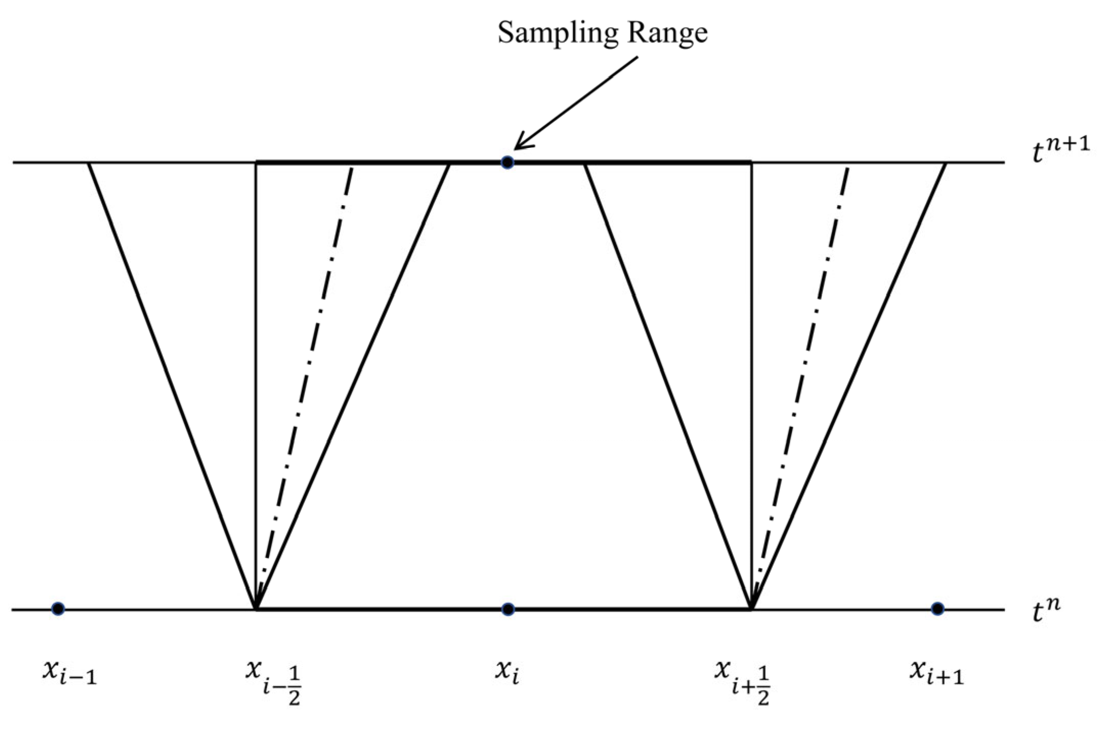
20]. This method selects an x-position of random sampling and obtains Riemann solutions of the next time level, illustrated in
Figure 2. To represent the value of
at the next time level, given the constant variables
of a cell
i at a time step
n, we can employ the following two steps:
Step I. Obtain the Riemann solutions and of the Riemann problems RP () and RP () at a general point (x, t).
Step
II. Perform a random sampling of solutions in the cell
i to obtain a state at time level
. The selected state is determined based on a random or quasi-random number
, which falls within the range of [0, 1].
Here, the van der Corput sequences are used to sample the solution [
21], and were found to provide the best results [
22].
One variation of the RCM involves a staggered grid and implements a two-step procedure. The non-linear systems’ solutions are obtained through the following two steps:
Step
I. Solve the local Riemann problems
and
, which are defined by the constant states
,
and
. These Riemann problems are solved to determine the intermediate states for each cell interface.
Randomly select local Riemann states; the solutions at time
are calculated and mapped onto a secondary grid. This secondary grid serves as a mid-point grid or an intermediate grid where the numerical calculations take place as follows:
Step II. Random-sample the Riemann problem defined by the data and , on the staggered grid. Subsequently, the solution is allocated to a new position at the time level , aligning with the position it occupied at time .
The final solution is written as
Based on the RCM mentioned before, a two-step scheme is introduced which enables the scheme to reach second-order accuracy in space. Using the framework of the finite difference method, in the first step, calculate the Riemann problems RP (
) and RP (
) to find the respective solutions,
,
. After that, random-sample the solutions at time
in a similar manner as in the RCM with a modified random number
, where
is the sequence of pseudo-random numbers in
. Next, with the solutions of
, the boundary fluxes of the cell i can be obtained, and
is advanced to
via the upwind scheme.
Therefore, this higher-order random choice method can be considered a random generalization of the two-step Richtmeyer form of the Lax–Wendroff scheme. Here, the Lax–Friedrichs scheme is replaced by the classical random choice method, and the second leap-frog type step is identical to the Lax–Wendroff scheme.
5. Discretization of Source Terms and Stability Constraints
The source term associated with the geometry in this study is incorporated into the solution via a time-splitting process, employing a second-order Runge–Kutta discretization which culminates in the ensuing explicit method.
Update with the source term by
:
Re-update with the source term by
:
where the evaluation of the source term
, which appears in Equation (8), requires the definition of the variable width and bottom, namely,
and the grid energy line slope
, which may be obtained from Manning’s equation, is as follows:
where
is the hydraulic radius and
is the Manning roughness coefficient.
The stability constraint of the model includes two parts: the Courant–Friedrichs–Lewy (CFL) criterion and the source term constraint. The CFL constraint criterion is provided here.
where
is he maximum Courant number at the time level
n. From Equation (30), the permissible time step for the convective part is given by
It can also be shown that the permissible time step for the source term is given by the following [
23]:
where the ratio of vectors
is defined as
. Since the same time step
must be used for the convective part and the source term,
must be used instead of
. Finally, the maximum permissible time step including the convective part and the source term will be given by
6. Numerical Validations and Discussion
This section describes the validation of the present model against various open-channel flow tests with different widths/bottom topographies. The gravitational acceleration used in all tests was 9.81 m/s2, and the Courant number value was 0.8. The model was tested against a range of scenarios to evaluate its ability to accurately simulate open-channel flows and to ensure its suitability for future applications.
6.1. Dam Break Tests
In this test, the accuracy of the presented model was evaluated via dam break (dry and wet beds) simulations without friction. The first test scenario involved simulating the sudden opening of a sluice gate separating two pools of still water. The two pools are located at different depths with a 1000 m long frictionless, horizontal channel. Two ends of the pools are closed borders which can be calculated via a reflection boundary in the entire numerical simulation. The initial conditions provide the following:
Figure 3 illustrates a comparison of the simulation results of the present and Godunov-type scheme (GTS) models, with the exact solution corresponding to the specified Courant number and grid size. The results of the simulation indicate that the present model has a great ability to handle discontinuities, particularly in case of the shock wave, where the resolution is more distinct compared to the Godunov-type scheme (GTS). For the rarefaction wave, the present model also shows a high level of accuracy, but wave oscillation appeared at the tail of the rarefaction wave.
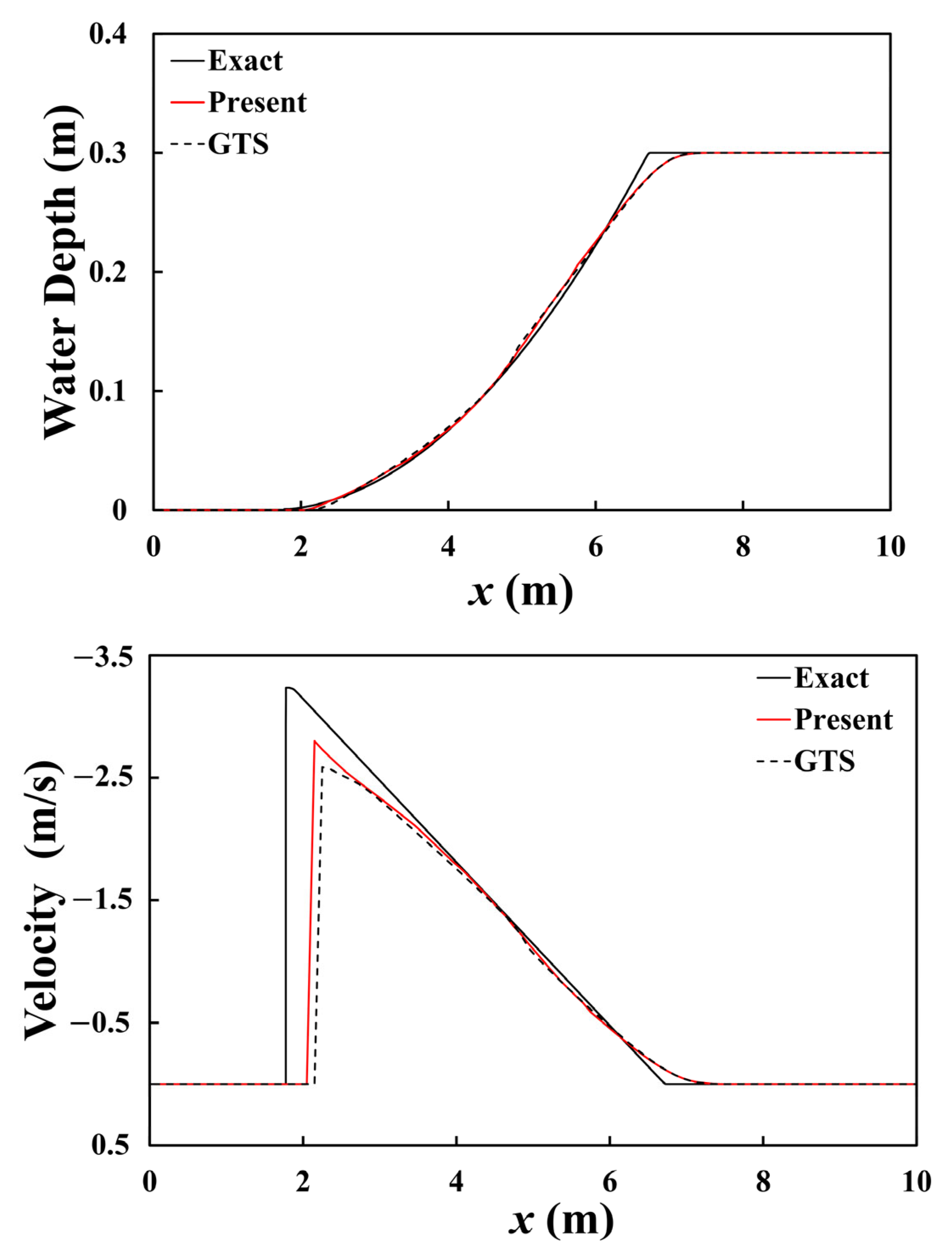
To evaluate the accuracy of the model for dam break flows in dry bed scenarios, we considered a specific test case. In this analytical case, there is a frictionless horizontal channel measuring 10 m in length. The computational domain is divided into two halves: the right half has an initial water depth (
h) of 0.3 m, while the left half represents a dry bed. At the beginning of the simulation, the water in the entire domain is in its initial state, with no motion. A Riemann solution of the dry bed in a shallow water flow is given in Equations (16)–(19). The water depth and velocity profiles at
t = 1 s with a given Courant number and grid size are shown in
Figure 4, respectively. As can be seen from the figures, the velocity profiles generated by the present model demonstrate good simulation capabilities at the dry–wet interface compared to the GTS. Actually, this demonstrates the advantages of the numerical scheme with the RCM currently employed. It allows for more accurate simulation results, especially when dealing with dry–wet interfaces.
6.2. Lobovsky et al.’s Dam Break ExperimentA
The second case in this section is about an experimental test, and a schematic of the experiment by Lobovsky et al. [
24] is presented in
Figure 5. The gray square area in
Figure 5 represents still water at the initial moment, and the left side of the region is a dry bed. The points labeled H1, H2, H3, and H4 indicate the specific locations at which the water level was measured. These points serve as reference points for monitoring and analyzing the behavior of the water level at different positions along the tank. More details on the experimental configuration and the apparatus utilized can be found in Lobovsky et al. [
24]. A comparison of the simulation results of the present model and the measurement data is shown in
Figure 6. The water depths were standardized by referencing the initial water depth
h = 0.3 m, and the time measurement on the
x-axis was adjusted by scaling it according to (
g/h)
1/2.
Compared with the scale of the experiment, the grid size selected here is relatively dense (
= 100). Based on the observations from
Figure 6, the simulation results are quite aligned with the measured values for the current model. The performance of the proposed model in this test is satisfactory, especially at the second peak of the four locations where very steep simulation results were achieved.
6.3. Laboratory Experiment of a Dam Break Flow over a Triangular Obstacle
A varying bed elevation is considered in this case. This test comes from the Concerted Action on Dam-break Modeling project (CADAM) [
25], which presents effective benchmarks for verifying dam break flow simulations. As depicted in
Figure 7, the experimental arrangement comprised a reservoir, a dam, and a rectangular channel measuring 38 m in length and 1.75 m in width. The dam separates the reservoir from a linear channel spanning 22.5 m in length. A symmetrical triangular elevation, measuring 0.4 m in height and extending 6 m in length, is located 28.5 m away from the upstream end. The channel is initially a dry bed with a constant Manning coefficient of
= 0.0125. In this test, the upstream end is assumed to be solid, and a chute is imposed downstream as a boundary condition.
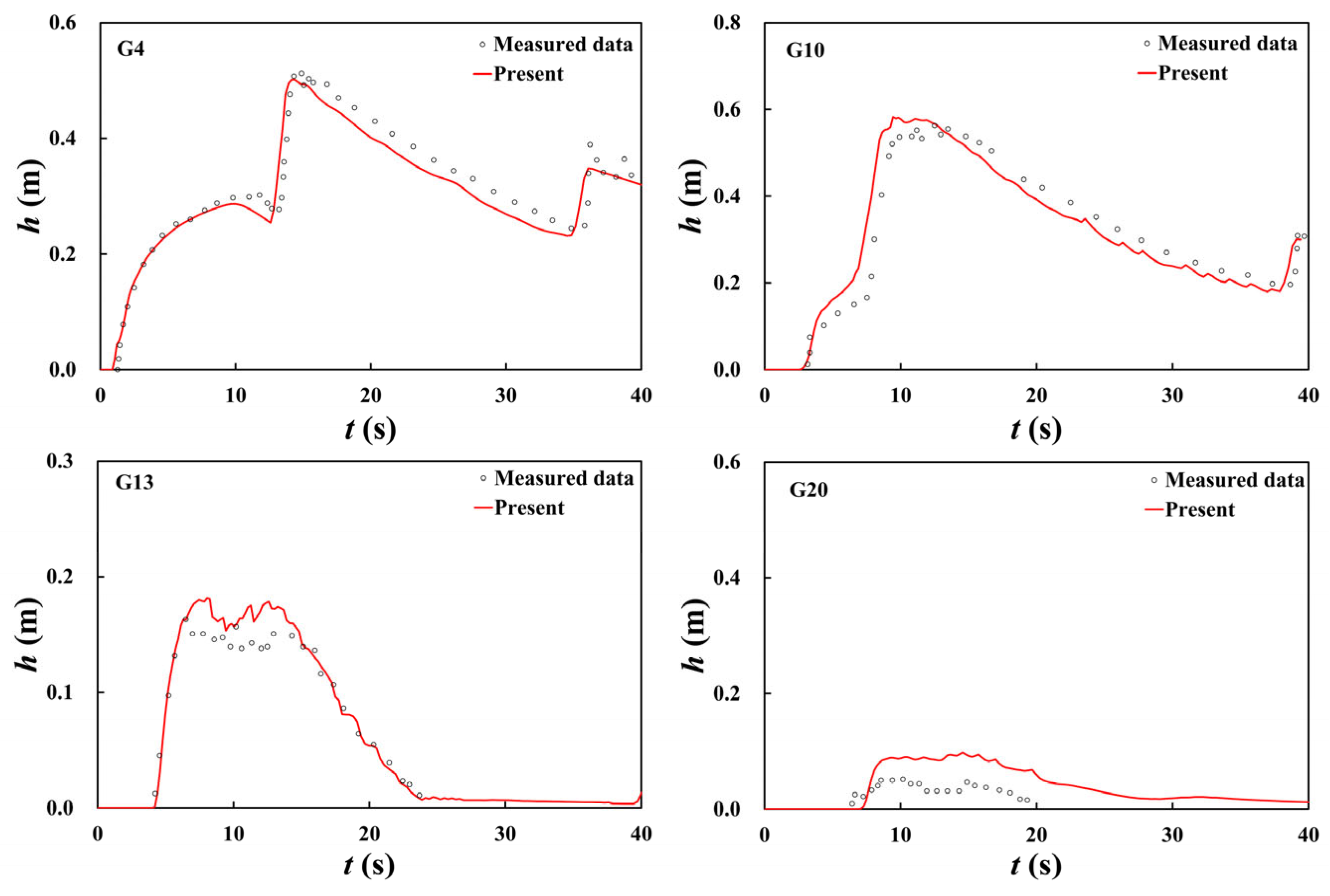
At the instant of the initial time, the dam experiences a sudden breach, causing the initially stagnant water in the reservoir to rapidly flow onto the floodplain downstream. As shown in
Figure 8, comparisons of the simulation results and experimental measurements were made at four gauges (G4, G10, G13, and G20). Several flow patterns can be observed in this test, like shock front propagation, a wet–dry front, partial reflections, and hydraulic jumps. The wet–dry front reaches location G4 about
t = 1 s after the dam breaks. At
t = 12 s, an increase in the incident water depth can be observed due to the shock wave. After that, a shock wave moving upstream forms because of the interaction between the incoming flow and the bump. As a result, a second increase in water depth can be observed at
t = 35 s. At the same time, a rarefaction wave is generated and propagates downstream, leading to a reduction in the water level above the hump.
It is proved in this figure that the comparison between the numerical predictions of the present model and the measurements yields satisfactory results at the gauge locations, and the transitions between dry and wet conditions are simulated with high precision. The current model produces oscillation issues; however, it accurately predicts the timing and maximum peak value of each of the two hydraulic surges. This confirms the effectiveness of the current method in dealing with a complex channel flow with non-uniform bed topography.
6.4. Dam Break Flow onto a Channel with a Local Constriction
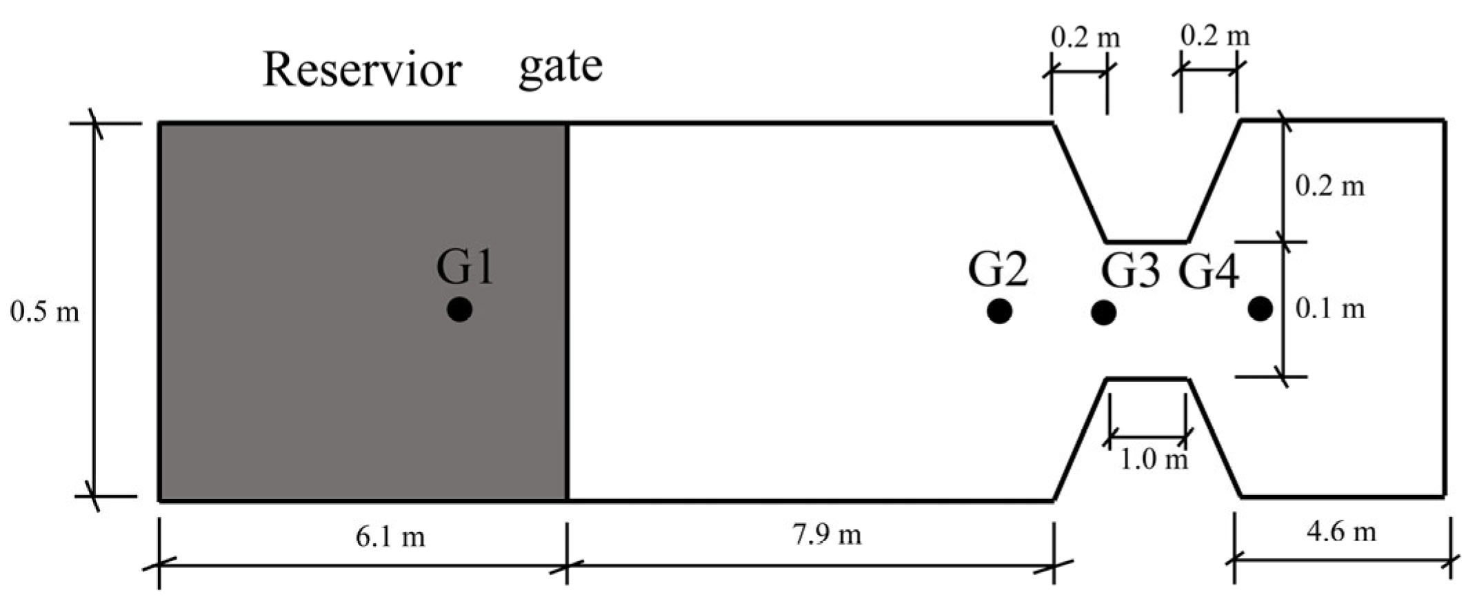
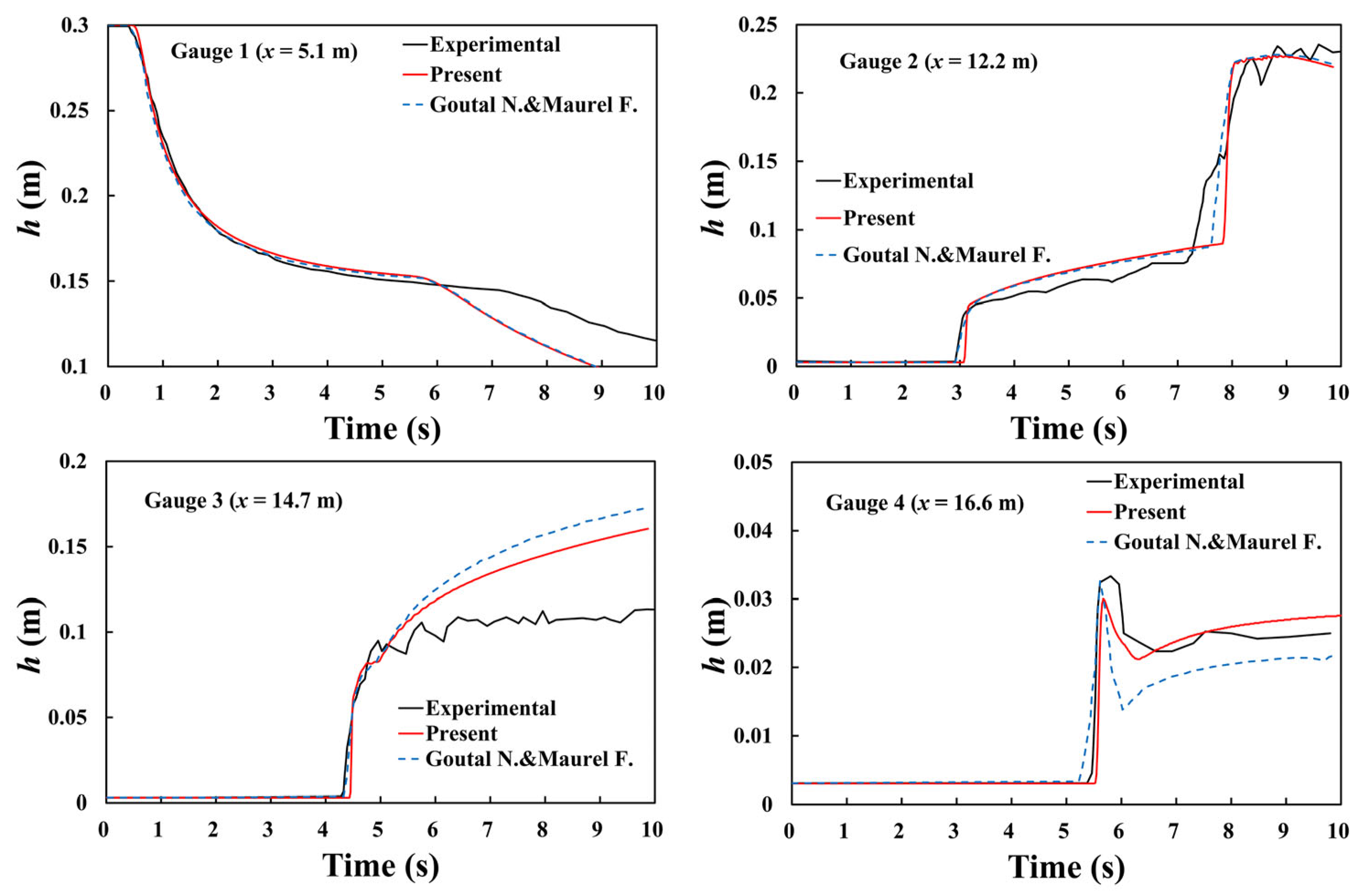
Figure 9 depicts the layout of a channel featuring a gate positioned at a distance of 6.1 m from the initial end of the upstream. At a starting point of 7.9 m beyond the gate, the channel, which is 0.5 m in width, gradually narrows down to a width of 0.1 m over a stretch of 0.2 m. The channel then sustains this width of 0.1 m for an extent of 1 m before returning to its primary width over a span of 0.2 m. The initial static water depths located upstream and downstream of the gate are noted as 0.3 m and 0.003 m, respectively.
In this test, the number of grid cells is set to 50, and a Manning coefficient of 0.01 is employed. The upstream boundary is assumed to be close, while the downstream boundary is set to be transmissive. The simulation was executed for a duration of 10 s following the collapse of the dam.
Figure 10 illustrates a comparison between the forecasted water depth profiles at four designated measurement points with experimental data from the laboratory tests and the corresponding numerical outcomes generated by Goutal, N., and Maurel, F. [
18].
The measuring points are positioned along the central axis of the waterway, as indicated in
Figure 9.
Gauge 1: 1.00 m upstream from the dam;
Gauge 2: 6.10 m downstream from the dam;
Gauge 3: 8.60 m downstream from the dam;
Gauge 4: 10.50 m downstream from the dam.
After the dam breaks, a surge of water is discharged downstream, propagating as a shock wave. Upstream of the dam, a rarefaction wave develops, resulting in a decrease in the water level, as depicted in
Figure 10 at Gauge 1. Gauge 2 experiences a sudden surge in water depth when the shock front arrives after approximately 3 s. At
t = 8 s, another abrupt change in depth is observed when the reflected shock from the narrow passage reaches the gauge. Inside the narrow passage at Gauge 3, only one sudden increase in water depth occurs. Downstream of the narrow passage at Gauge 4, the water level experiences a sudden increase caused by the incoming pressure surge, after which it drops to a relatively stable level.
The present model and the predictions made by Goutal, N., and Maurel, F., are quite similar. Especially at Gauge points 3 and 4, the predicted water depth ofthe present model after 7 s is more consistent with the experimental data than the results from Goutal, N., and Maurel, F.. Overall, this test validates the model in dealing with a complex channel flow with a varying width.
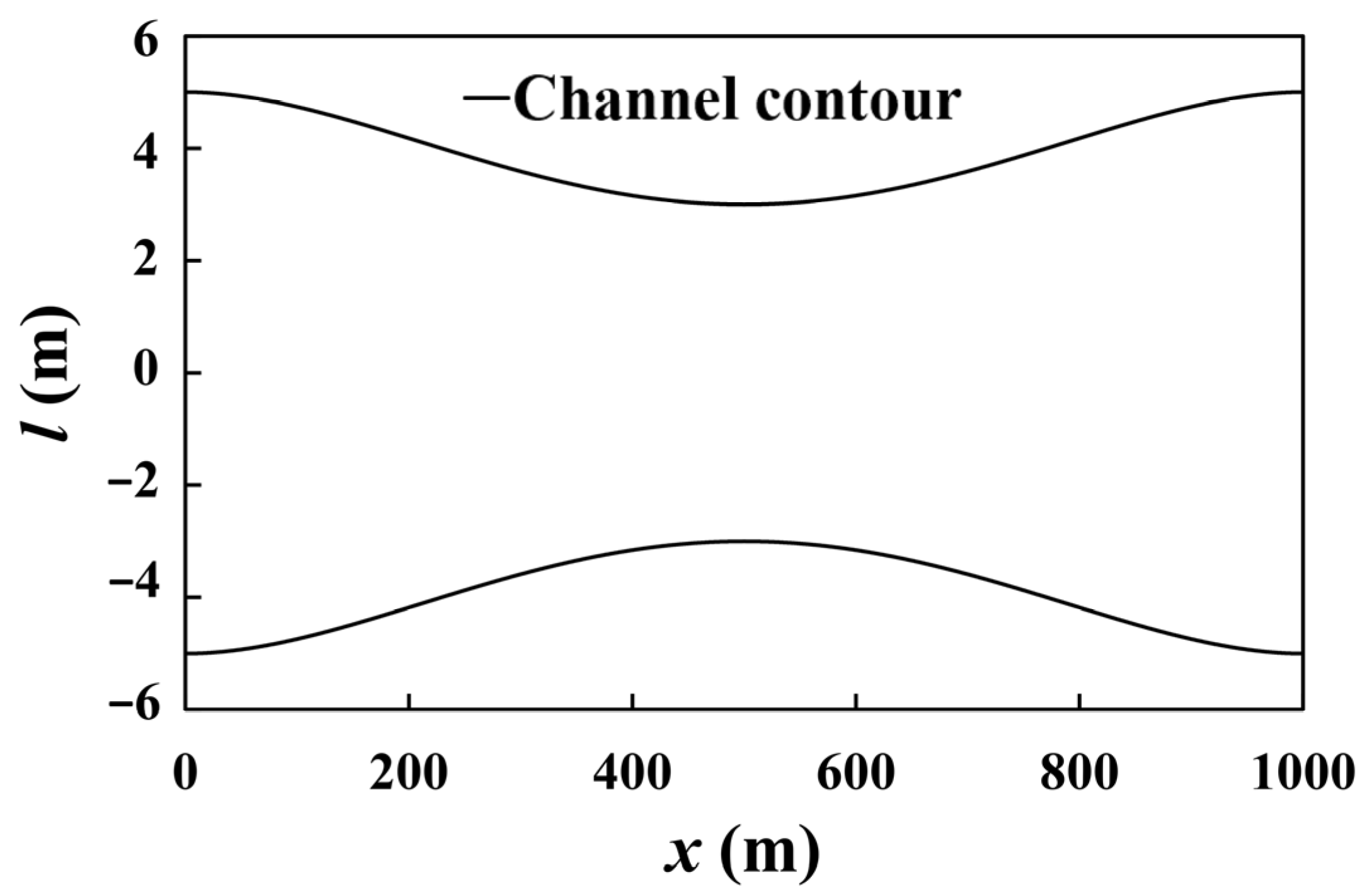
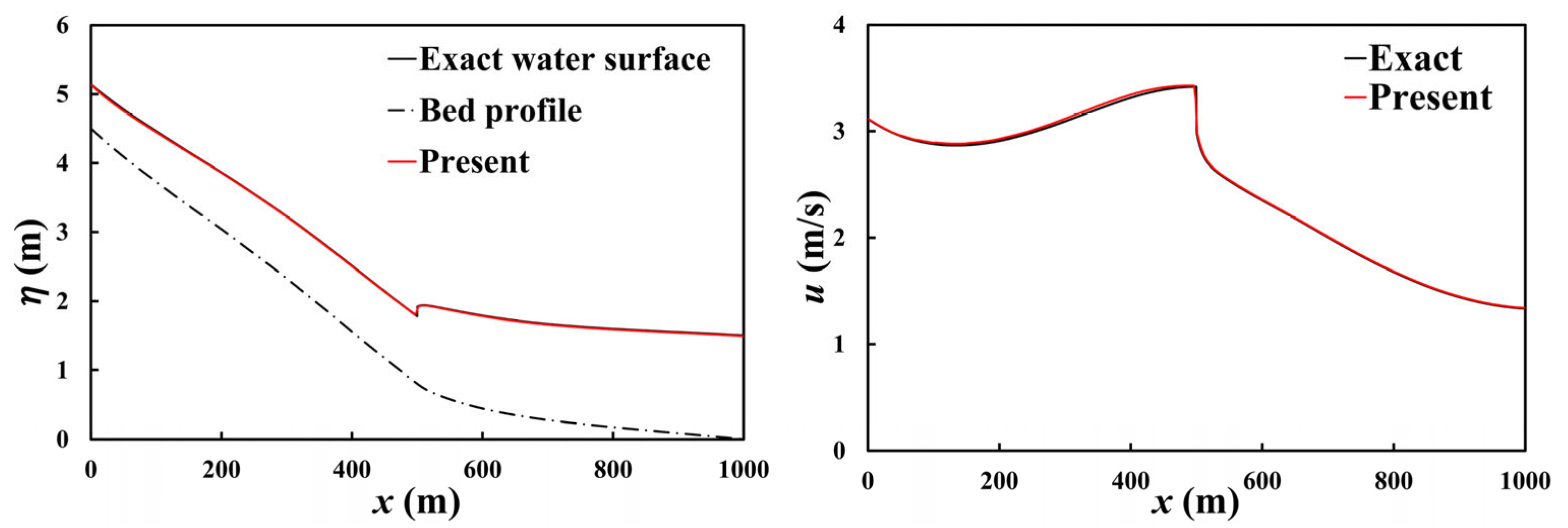
6.5. Channel Contraction Test Problem
To validate the numerical schemes, simulations were conducted to replicate a set of steady flows in domains with changing topographies. This specific quasi-equilibrium flow issue was introduced by MacDonald et al. [
26] and is widely recognized as a benchmark for assessing numerical schemes. It involves all source terms described by Equation (8), which includes diverse channel widths, changing bed elevations, and frictional effects.
The flow occurs in a channel with a length of 1000 m and exhibits specific analytical characteristics. The depth variation features a hydraulic jump located at the mid-point of the channel and is expressed as a function of the horizontal coordinate
x.
where
,
= −0.230680,
= 0.248267, and
= −0.228271.
As shown in
Figure 11, variable channel width is given by
And the friction term
is
The particular data for this test case include a Manning resistance coefficient of
and the physical boundary conditions for this simulation include an upstream discharge of 20 m
3/s and a downstream water depth of 1.5 m. The discretization of the channel is accomplished using a uniform grid spacing of
= 2.5 m. The simulation was initialized using these specific boundary and initial conditions, and the simulation ran until a steady state was reached. The exact bed elevation, water surface level, and velocity profiles obtained from the numerical simulation are plotted in
Figure 12, and they show a good agreement with the expected analytical profiles. The evaluation of numerical and analytical profiles is an essential step in validating the precision of the numerical approach used in the simulation. The predicted free surface level matches the analytical profiles, indicating that the current model has achieved a satisfactory level of accuracy for simulating steady flows.
7. Conclusions
In this paper, a novel model was proposed for simulating a 1D open-channel flow with a changing width and bed profile. For the hyperbolic problems in the homogeneous system, a higher-order RCM in the framework of an upwind scheme was used by sampling a local Riemann solution state at random with an HLL Riemann solver. The Runge–Kutta scheme was introduced for the discretization of the source term of the system to achieve second-order accuracy and ensure accurate numerical simulations.
To test the proposed model, five specific tests were carried out. These tests encompassed dam break flow tests and different configurations involving variable widths, bottom elevations, and frictions. The first test focused on the simulation of an unsteady dam break flow in a flat bed channel under both dry and wet downstream conditions for which the presented model was evaluated compared to the Godunov-type scheme and the exact solutions. The second, third and fourth tests were unsteady dam break tests that considered the source term, and the calculation results of the presented model were compared with the experimental data. The last test was a steady flow test including a varying channel width, changing bed elevation, and friction, which was used to verify the stability of the model. The main findings of the proposed model can be summarized as follows:
(1) The present model has a great ability to handle discontinuities, especially in the shock wave or the dry–wet interface, which exhibits a higher level of resolution compared to the Godunov-type scheme (GTS). For the rarefaction wave, the present model also shows a high level of accuracy, but wave oscillation appeared.
(2) By comparing the experimental results, the performance of the proposed model is found to be satisfactory, particularly in accurately simulating dry-to-wet transitions. The presented model produces oscillation issues but achieves accurate predictions for the timings and maximum peak values of the hydraulic surges. These confirm the effectiveness of the current method in presence of source term discretization.
(3) The simulated free surface level matches precisely with the analytical profiles while maintaining satisfactory accuracy for steady discharge solutions in the steady flow test. This demonstrates the ability of the presented model to handle source terms and to maintain equilibrium for a steady flow.
The proposed model is inherently accuracy and stable, and it deserves further research and application.


