Probabilistic Analysis of Floods from Tailings Dam Failures: A Method to Analyze the Impact of Rheological Parameters on the HEC-RAS Bingham and Herschel-Bulkley Models

Abstract

The difficulty in determining the rheological characteristics of tailings inside reservoirs as well as their intrinsic variability adds uncertainty to tailings dam failures in flood studies. Uncertainty propagation in non-Newtonian hydrodynamic models stands as a great scientific challenge. This article explores the sensibility of tailings dam breach flood mapping to rheological parameters in Bingham and Herschel-Bulkley (H-B) models. The developed approach was based on the probabilistic Latin Hypercube Sampling of rheological parameters. It was automated to propagate uncertainty throughout multiple hydrodynamic simulations using the HEC-RAS v.6.1 software. Rheological parameter ranges and distributions were based on a broad bibliographic review. Bingham models were revealed to be more sensitive than H-B in terms of simulated min-max area values: for Bingham, flood areas, maximum depths, and arrival times varied by 17.9%, 9.3%, and 8.2%, respectively; for H-B, variations were 25.7%, 5.1%, and 3.9%. However, Bingham was less sensitive in terms of hydrodynamically associated probability: high probability ratios were related to a small range of simulated areas in Bingham, while H-B presented great variability. Finally, for each model, the parameters that affect uncertainty the most were identified, reinforcing the importance of determining them properly. Furthermore, the identified parameter ranges for both models should be valuable for defining variable value boundaries for flood sensitivity tests on specific tailings materials for other case studies. The automated algorithm can be used or adapted for specific tests with other hydrodynamic simulations.

1. Introduction

Failures of tailings dams occur at a significantly higher frequency compared to those of water storage dams [1]. Recent incidents have highlighted the immense destructive potential associated with tailings inundations [2,3]. Forecasting and mapping flood hydrodynamics are crucial for implementing effective risk mitigation measures. Different uncertainties may impact flood risk assessments. During the last decade, the simulation of floods resulting from tailings dam failures has commonly been performed using Newtonian models. However, the tailings comprise a combination of fine materials and water, and depending on the proportions in terms of solid concentration, their properties can resemble non-Newtonian fluids (hyper-concentrated), which brings uncertainty to dam-break studies.

Rheology investigated the flow and deformation behavior of fluids in different contexts [4,5]. Rheological parameters are obtained and analyzed through rheological tests conducted on various materials over time [6,7,8]. Several factors can influence the variability of rheological parameters, including shear rate, solid concentration, pH, and temperature [9]. The effects of physical and geotechnical parameters on rheological properties were also evaluated [10]. Different models have been employed for simulating hyper-concentrated flows for decades [11,12,13].

The term “hyper-concentrated flow” commonly refers to natural mudflows or debris flows [14]. Numerous investigations have delved into the influence of rheological parameters on the natural flow of mud, particularly debris flow [15,16,17,18,19,20,21,22]. These studies yielded good results when compared to recorded events. However, for predictive applications, it is widely recognized that the difficulties in determining representative rheological parameters, along with their considerable spatial variability, remain significant sources of uncertainty in this type of model [17,23,24]. Notably, the authors in [24] conducted a sensitivity analysis of non-Newtonian hydrodynamic modeling of debris flow with regards to rheological parameters, highlighting the relevance of these parameters in hydrodynamics.

Over the course of time, numerous in-depth investigations have been undertaken to explore various dimensions of this uncertainty. Specifically, the author in [25] investigated the uncertainties inherent in physical and rheological parameters during the numerical simulation of non-Newtonian flow phenomena. The authors in [26] focused on the examination of uncertainties pertaining to input parameters employed in the modeling of natural soil landslides within steep terrains. Moreover, the authors in [27] evaluated the parameter variability concerning the uncertainties associated with rheological characterization. These studies highlighted the relevance of rheological characterization for hydrodynamic analyses.

Sensitivity analyses have also been applied in the study of rheology, with methods such as the Monte Carlo Method (MCM) being used to investigate various scenarios, including mudflow and natural debris events [26,28] and pipeline and pump flows associated with tailings transportation [29]. The studies encompassed the utilization of Bingham models [26,28,30] and the Voellmy model [26]. In contrast, the authors in [24] uniquely conducted a global sensitivity analysis of the Quadratic model in FLO-2D software, employing Latin hypercube sampling (LHS), to evaluate the impact of rheological parameters on natural mudflows.

Despite the numerous studies that have focused on these parameters in the context of debris flows, limited attention has been given to their investigation in the context of tailings dam failures. Studies that performed sensitivity assessments of the rheological parameters linked to tailings dam failure, the specific subject of this article, have not been found. Despite the potential similarity in behavior between flood wave propagation in tailings dam failures and debris flows, there is currently a lack of studies specifically focusing on the propagation of uncertainties in the hydrodynamic modeling of tailings dam failure floods. In this context, the significance of the pronounced variability of rheological parameters is underscored among the challenges associated with the modeling of tailings dam failure floods. With the purpose of filling this scientific gap, this article explores rheology uncertainty in the context of dam-break studies.

Currently, several hydrodynamic models allow for the simulation of hyper-concentrated flow and are already being used for dam-break studies, such as FLO-2D [15,24,31,32], RIVERFLOW2D [33], and FLWAV [34]. Recently, the widely used and freely available program HEC-RAS has also incorporated non-Newtonian flow modeling. However, sensitivity studies of HEC-RAS to rheological parameters in the modeling of hyper-concentrated flow, particularly for tailings dam failures, have not been performed.

In order to assess the effects of rheology uncertainty and to explore the applicability of the HEC-RAS model for practical purposes related to mapping floods with hyper-concentrated flow, this study seeks to address the following question: How does the rheological variability of stored materials impact the results of modeling floods caused by mining tailings dam failures? To address this question, this article presents a probabilistic method to analyze the sensitivity of flood maps to input parameters of the HEC-RAS Bingham [35] and Herschel-Bulkley [36] rheological models, which are the most adapted rheological models for hyper-concentrated flow simulations [9,27,37]. Within this context, the developed research compares the influence of rheological characterization in both models, raising the question of the suitability of these models for dam-break analysis regarding uncertainty boundaries. For this purpose, ranges of variation for rheological parameters were explored based on an extensive literature review and through a case study probabilistic analysis. Thus, this study demonstrates the importance of rheological characterization in dam-break studies and introduces a probabilistic method to assist in the analysis of rheological parameter uncertainties due to the heterogeneity of tailings materials.

2. Materials and Methods

The sensitivity analysis proposed in this research is based on four main steps: (1) definition of test parameters; (2) literature review of parameter ranges and probabilistic sampling; (3) automated downstream propagation simulations of the rupture wave; (4) compilation and analysis of results.

The Bingham and Herschel-Bulkley models were tested, and the Latin Hypercube Sampling (LHS) technique was used to randomly sample the rheological parameters under investigation based on a comprehensive literature review. The sensitivity analysis is applicable to any deterministic hydrodynamic model developed using the HEC-RAS framework, that encompasses the propagation of wave rupture in tailings dam scenarios. Similar to the existing approach [24], the impact on flood extent and maximum depth was also assessed. Additionally, the analysis encompassed the examination of flood wave arrival times, considering the significant importance of this parameter in studies concerning impacts and loss of life [38,39]. The automated repetition of these steps is determined by the parameters being tested and the sampling approach. The developed sensitivity analysis was applied to the conceptual case study conceived and analyzed in [40], proposed by the International Commission on Large Dams (ICOLD).

2.1. Mathematical Rheological Models and Parameterization

Given the nonlinear relationships between shear stress and strain rate, several mathematical models were developed to represent the behavior of non-Newtonian fluids [14,35,36,41,42]. Laboratory experimental results [43] cited in the study [4] confirmed that under deformation rates observed in the field, fluids with high concentrations of fine particles exhibit plastic behavior resembling Bingham fluids. In this context, the rheological models commonly used to represent the flow resulting from the rupture of ore tailings dams are the Bingham and Herschel-Bulkley models [9,24,27,37].

The Bingham model, applied to plastic fluids, was developed in 1922 based on its conceptualization of the yield limit phenomenon, where a residual shear stress value must be exceeded for the material to flow. The Bingham plastic model tends to remain undeformed under the application of small shear stresses [44], represented by the sum of yield and viscous stresses, as given by Equations (1) and (2) [35].

$${\mathsf{\tau }=\mathsf{\tau }}_{\mathrm{y}}+\mathsf{\mu }\frac{{\mathrm{dv}}_{\mathrm{x}}}{\mathrm{dz}}{,\mathsf{\tau }>\mathsf{\tau }}_{\mathrm{y}}$$

(1)

$$\frac{{\mathrm{dv}}_{\mathrm{x}}}{\mathrm{dz}}{=0,\mathsf{\tau }<\mathsf{\tau }}_{\mathrm{y}}$$

(2)

where τ is the shear stress; τ_y is the yield stress or limit stress; µ is the dynamic viscosity of the mixture or dynamic viscosity; and dv_x/dz is the strain rate or velocity gradient.

Pseudoplastic fluids with yield stress can be represented by the Herschel-Bulkley model. This model, also known as the “generalized Bingham model”, was developed based on the Bingham and Power-Law models, aiming to incorporate the non-linear flow curve for stresses higher than the yield stress τ_y [45]. In this model, the shear stress and strain rate exhibit a non-linear relationship, serving as a generalized proposition of the Bingham plastic fluid. This relationship is described by Equations (3) and (4), indicating the sum of yield and viscous/turbulent stresses [46].

$${\mathsf{\tau }=\mathsf{\tau }}_{\mathrm{y}}+\mathrm{K}{\left(\frac{{\mathrm{dv}}_{\mathrm{x}}}{\mathrm{dz}}\right)}^{\mathrm{n}}{,\mathsf{\tau }>\mathsf{\tau }}_{\mathrm{y}}$$

(3)

$$\frac{{\mathrm{dv}}_{\mathrm{x}}}{\mathrm{dz}}{=0,\mathsf{\tau }<\mathsf{\tau }}_{\mathrm{y}}$$

(4)

The relationship between shear stress and strain rate depends on the dimensionless exponent n, which is specific for each fluid and determined experimentally [44]. This coefficient is the same as the behavior index in the Power Law model. In addition to the flow behavior index n, the consistency index K in the Herschel-Bulkley model is also an empirical parameter [6].

HEC-RAS has four rheological models in its structure [46]: the Bingham model, which is standard for hyperconcentrated flows; the O’Brien (Quadratic) and Generalized Herschel-Bulkley models for mud and debris flows; and the Clastic-Grain Flow model (Mohr-Coloumb geotechnical model) for clastic flows.

In this research, the test parameters were defined according to the input data of the non-Newtonian fluid modeling in HEC-RAS for the Bingham and Herschel-Bulkley rheological models. The following parameters were defined for the Bingham model: volumetric concentration of solids (C_v); maximum volumetric concentration of solids (Max C_v); and the coefficients a and b of the exponential yield stress curve. These parameters were determined in view of the predefined HEC-RAS approaches. For the Herschel-Bulkley model, the following parameters were defined: the yield stress (τ_y), the consistency index (K), and the behavior index (n). In this case, the predefined approach of the exponential curve, i.e., the calibration parameters a and b, was not used since these parameters are usually adjusted based on the yield stress (τ_y) of the Bingham model. Thus, Herschel-Bulkley yield stress (τ_y) values obtained from previous studies were used.

2.2. Parameter Intervals and Sampling

To conduct the sensitivity tests in this study, parameter value ranges for the equations were determined based on an extensive literature review related to mining tailings [2,7,8,9,10,14,27,37,38,47,48,49,50,51,52,53]. The tailings studied by these authors included coal, copper, iron, lithium, base metal, nickel, gold, pyrophyllite, uranium, and zinc, as well as synthetic and theoretical materials, and the obtained values are listed in Appendix A. Although there are limited studies on tailings rheology analysis, the identified intervals served the purpose of constituting a sample space that allowed for the variation of values and the evaluation of their influence.

The establishment of physically plausible value ranges for the rheological parameters of interest was performed (

Table 1. Value ranges of rheological parameters defined for the sensitivity assessment of HEC-RAS using Bingham and Herschel-Bulkley models.

Rheological Model	Varied Parameters	Literature Value Ranges	Adopted Interval
Bingham	Cv (%)	9.3–65.0	20.0–60.0
	Max Cv (%)	49.9–76.5	49.0–61.5
	a (Pa)	0.0000001–3.45	0.067–3.450
	b	1.2–40.0	1.2–10.359
Herschel-Bulkley (H-B)	Cv (%)	20.0–60.0
	τy (Pa)	0.6–251.9
	K (Pa∙sn)	0.008–130.0
	n	0.192–1.5

) based on the provided literature review (Appendix A).

In the case of the Bingham model, the parameters C_v, Max C_v, a, and b were subject to variation. The decision to employ independent random sampling for these parameters is justified by the inherent limitation of HEC-RAS, which utilizes a fixed C_v value. Consequently, the resulting values of yield stress (τ_y) and dynamic viscosity (μ) remain constant when C_v is employed in their calculation. Additionally, to ensure physically meaningful parameter combinations, the value ranges and relationships between the parameters were adjusted to yield τ_y and μ values within the ranges documented in the literature (Table 1), following a similar approach [24].

To encompass the classification of flow types proposed by the authors [54], the interval for solid volume concentration (C_v) in the context of hyperconcentrated flow was defined as 20% to 60%. This interval was chosen to cover a range of flow conditions, including floods, mudflows, and hyperconcentrated flows. Based on the literature, the study [54] suggested a C_v range of 20% to 50% for floods and mudflows, while [54] proposed a C_v range of 30% to 60% specifically for hyperconcentrated flows.

In relation to the maximum volumetric concentration parameter (Max C_v), the chosen interval considered a maximum value of 61.5%, which corresponds to the value reported in [53]. This value is pre-defined in HEC-RAS [46], and since it exceeds the upper limit of the adopted interval for solid volume concentration (C_v of 60%), it was established as the maximum value for the Max C_v interval.

The values of C_v and Max C_v were independently sampled, along with the parameters a and b in the Bingham model. Subsequently, the sampled values of Max C_v were reorganized to ensure that within each parameter set, the value of Max C_v was always greater than C_v. Another criterion in combining these parameters was to adhere to the limits of dynamic viscosity (μ) reported in the literature, with a minimum μ of 0.002 Pa∙s [9] and a maximum μ of 100.0 Pa∙s [38]. In brief, the Max C_v samples were rearranged, based on the C_v samples, in such a way that the relationship between the parameters satisfied two criteria: Max C_v > C_v, and the relationship between Max C_v and C_v in the calculation of μ using the Maron and Pierce method [46] yielded values within the range of 0.002–100.0 Pa∙s.

The values of a and b in the yield stress curve were adjusted to ensure that the combination of parameters yielded values within the range of 0.085 Pa [49] to 1726.33 Pa [48]. The value of 2396.53 Pa presented in Appendix A as the maximum value from the study [48] is related to a C_v of 65% in the slump test. In accordance with the C_v range of 20% to 60% adopted in this study, the value of 1726.33 Pa was considered the maximum value for τ_y, also obtained in the slump test for a C_v of 60%.

The parameters that varied in the Herschel-Bulkley (H-B) model were C_v, τ_y, K, and n. For this test, the ranges defined in the literature review (Table 2) were maintained, as the parameters K and n are calibration parameters of the H-B model and do not have a direct relationship that allows for evaluating or limiting their ranges. The range of solid volume concentration (C_v) was kept from 20% to 60% [14,54].

Similarly, the range of τ_y values in the H-B model remained the same as observed in previous studies. Although they share the same name, the yield stresses of the Bingham and H-B models have different values for the same fluid. Thus, the adopted yield stress range considers only the values adjusted according to the H-B model.

The random sampling of parameters using Latin Hypercube Sampling (LHS) was performed independently with the aim of analyzing the sensitivity of HEC-RAS to the parameters within their variability intervals. A total of 1000 parameter sets were selected for the simulations of each model, as the random sampling conducted by LHS allows for a reduced number of samples compared to the Monte Carlo method [55]. To achieve convergence in the Monte Carlo simulation, other authors have employed 5000 [26,29] and 10,000 [25] realizations, respectively. LHS is a statistical method [56] that generates a quasi-random sample of parameter values from a multidimensional distribution. In LHS, each variable set is divided into equal intervals, and one value is obtained for each stratum [56]. Assuming these variables are independent, the sample sets are randomly combined with each other, forming a multidimensional sample [56].

To obtain a set of samples generated by the LHS, it is necessary to adopt a probability distribution for each parameter to be varied. Few studies have evaluated the best-fit distributions for the variations in rheological parameter values. The research in [25] and the more recent work [30] considered that the dynamic viscosity (μ) follows a normal distribution. The probability distribution of the volumetric concentration of solid particles (C_v) in tailings was compared to the normal distribution using measured data [57]. The authors in [27] fitted normal, lognormal, gamma, and beta statistical distributions for rheological parameter sets. Due to the scarcity of studies and data used in fitting probability distributions in the literature for these parameters, the approach in [24] was adopted in this paper, which used a uniform distribution to account for the variation of all rheological parameters tested.

2.3. Automation of Sensitivity Analysis in HEC-RAS

To conduct probabilistic analysis, it was necessary to automate the modeling processes due to the repetitive nature of sampling and simulation. The automation of simulations in HEC-RAS was based on the principles exposed in [58] and achieved using HEC-RASController v.6.1, which is part of the model’s programming interface and consists of a collection of subroutines and functions in Visual Basic [59]. HEC-RASController can be used with Visual Basic for Applications (VBA), but according to [60], this programming language has limited usage, albeit highly useful. Consequently, other languages such as MATLAB and Python have been implemented in the HEC-RASController [60,61,62]. In this investigation, the automation of the four methodological steps: (1) sampling parameters with LHS and uniform distribution using the SCIPY.STATS library; (2) changing rheological parameters by editing the file “unsteady flow” (.u01) in text format; (3) simulation via HEC-RASController; and (4) Storing the results of flooded area, maximum depths, and arrival times using the H5PY library, was implemented using Python based on the same principles exposed by [58] to achieve a probabilistic full 2D and complete hydrodynamic model propagation algorithm.

Following the proposed methodology for sensitivity analysis, the developed computational routine (code provided in Appendix B) begins with Step 1, generating the sampling for each parameter to be varied. Contrary to [58], the developed algorithm for sampling was performed using the Latin Hypercube Sampling (LHS) method, similar to [24]. These tests with associated probability distributions (uniform) were performed using the SCYPY.STATS library in Python.

For achieving Step 2, the parameterization of the hydrodynamic model is done by modifying the “unsteady flow data” file (extension .u01), which stores input data, including the rheological parameters, as a text file.

After modifying the parameter set, simulations (Step 3) are performed using functions from HEC-RASController, opening and running the project with the altered parameters. Following each simulation, in Step 4, the results of the flooded area, maximum depths, and arrival times in each cell of the 2D model are stored using the H5PY library in HDF files, which allow for the organization and storage of large amounts of numerical data (such as matrix data).

Finally, upon completion of each simulation, the Python code generates the following outputs: the extent of the flooded area in a vector file, which is utilized to determine the flooded areas; maximum depths and arrival times derived from the “unsteady flow analysis” file (extension .p01) of HEC-RAS, encompassing the results for each cell of the model; relative errors in volume balance to assess potential instabilities in the simulations that could influence the results and consequently should be disregarded. With these results, it is possible to assess the sensitivity of the hydrodynamic model by observing the impacts caused by varying each rheological parameter. All Python codes developed are provided in Appendix B and can be used or adapted for other studies where automation is feasible.

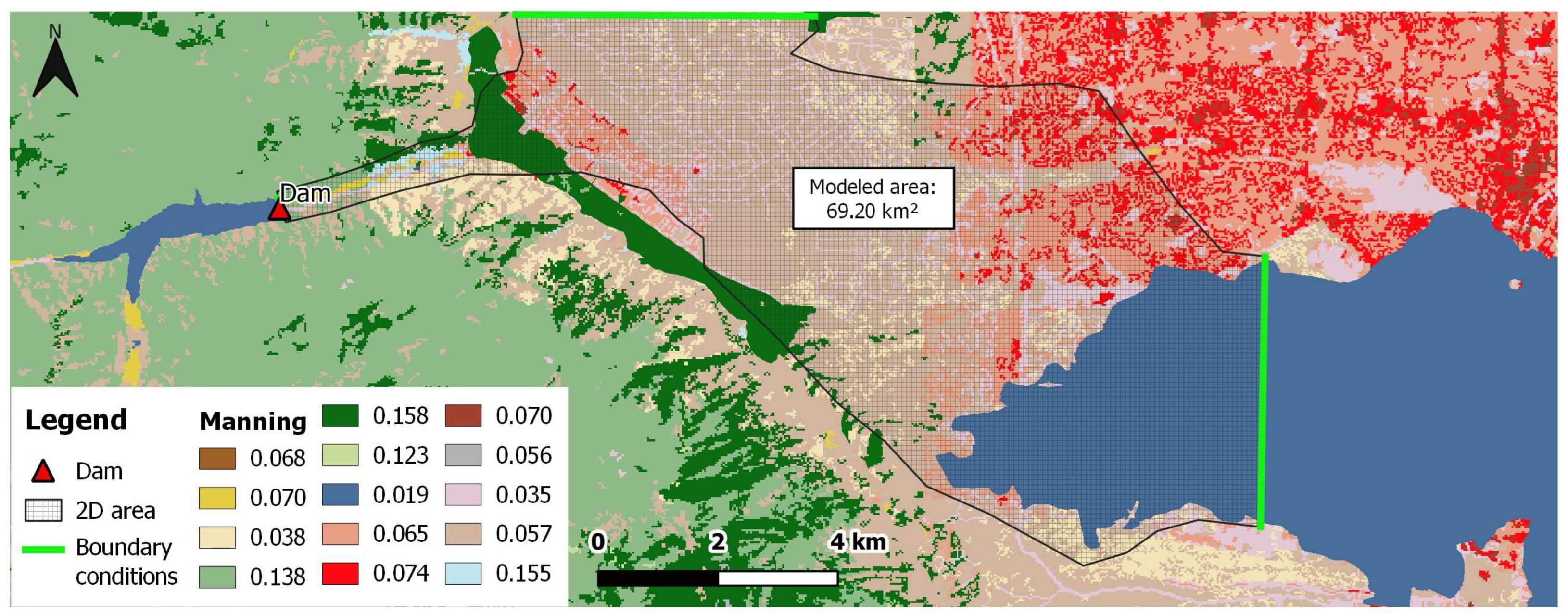
2.4. Case Study: The Hydrodynamic Model

The sensitivity analysis methodology developed in this study was applied to the ICOLD case study, which involves a hypothetical dam presented by [40], and was adapted here for the proposed testing purpose. This fictional dam is implemented in a virtual environment and has undergone extensive testing in a study conducted by the International Commission on Large Dams (ICOLD), which was presented at the 12th International Benchmark Workshop on Numerical Analyses of Dams. Eight studies evaluating the risks associated with the dam’s failure under different methodologies were published, and these studies were compiled by [40]. More recently, other studies have conducted dam failure analyses using the same case study [58,63]. None of these studies focused on rheological aspects, which is a novelty promoted by the present study.

The fictional dam has a height of 61 m (Elevation 272 m), upstream and downstream slopes of 3:1, a base width of 416 m, and a crest width of 24 m. The crest length is 360 m, forming a reservoir with a capacity of 38 × 10⁶ m³. It is located in a virtual mountainous terrain, with a confined V-shaped downstream valley along the first 3.6 km and a flat-floored urban area valley ending in a lake along approximately 17.6 km. It should be noted that for this study, it was assumed that the dam is an earth dam storing undefined mining tailings.

The Digital Elevation Model (DEM) used has a horizontal resolution of 9.5 m. The classification of land use and land cover, along with the assignment of Manning’s roughness coefficient values, is based on 14 typologies (Figure 1): open water (0.019); low-intensity open space developed areas (0.065); medium-intensity open space developed areas (0.074); high-intensity open space developed areas (0.070); barren land (0.056); deciduous forest (0.138); evergreen forest (0.158); mixed forest (0.123); shrubs (0.057); grass (0.038); pasture (0.070); cultivated land (0.068); and wetlands with shrubs (0.155) [40].

Table 2. Breach parameters calculated based on Froehlich.

Parameters	Data	Froehlich [64]
Failure Mode		Overflow
Total volume (Vw) (1.000 m3)	38,276.34
Average breach width (Bm) (m)		116.27
Minimum breach width (m)		55.27
Elevation of the dam crest (m)	272.00
Elevation of the base of the dam (m)	211.00
Elevation of the bottom of the breach (m)	211.00
Dam height (m)	61.0
Height of the breach (Hb) (m)	61.0
Time of breach formation (h)		0.54
Left Lateral Slope (H:1V)		1.0
Right Side Slope (H:1V)		1.0
Mode of progression		Sine Curve

Table 2. Breach parameters calculated based on Froehlich.

Parameters	Data	Froehlich [64]
Failure Mode		Overflow
Total volume (Vw) (1.000 m3)	38,276.34
Average breach width (Bm) (m)		116.27
Minimum breach width (m)		55.27
Elevation of the dam crest (m)	272.00
Elevation of the base of the dam (m)	211.00
Elevation of the bottom of the breach (m)	211.00
Dam height (m)	61.0
Height of the breach (Hb) (m)	61.0
Time of breach formation (h)		0.54
Left Lateral Slope (H:1V)		1.0
Right Side Slope (H:1V)		1.0
Mode of progression		Sine Curve

The computational domain of the developed model in HEC-RAS covers an area of 69.8 km². The computational mesh consists of cells with dimensions of 50 × 50 m, with a refinement of 40 × 40 m in the downstream thalweg of the confined valley, and cells of 100 × 100 m in the lake area. The downstream boundary conditions are defined as normal depth in two sections, with a slope of 0.005 m/m for the thalweg and 0.0001 m/m for the downstream lake. The computational time step used in the simulations was one second, satisfying the Courant condition with a maximum value of unity. The shallow water equations (SWE) were employed to perform the simulations.

The flood hydrograph used in the analysis was obtained using the parametric model proposed by Froehlich [64], which is widely applied for defining dam failure debris flow. No considerations were made for breach formation and mobilized volume parameter variations. The theoretical failure mode assumed the complete opening of a breach with a height equal to the height of the dam. The calculated parameters can be observed in Table 2.

After the parameter calculation, the obtained values were integrated into the HEC-RAS software to derive the rupture hydrograph, representing the flow characteristics ensuing from breach initiation and subsequent reservoir discharge. The analysis yielded a peak flow rate of 37,826.19 m³/s.

3. Results

The sensitivity evaluation was performed according to the results of each simulation. A total of 2000 simulations were performed, 1000 with the Bingham model and 1000 with the Herschel-Bulkley (H-B) model.

The results obtained were evaluated in terms of flooded area, maximum depths, and arrival times. To analyze the results of the 2000 simulations, percentage coefficient of variation (COV), Spearman’s rank correlation coefficient, and histograms were used. The details of these results are presented in the following sections: A summary for each model with the computational specifications of interest for the probabilistic simulations is presented in Appendix C. Complementary exhaustive result sets analyzed in relation to their variability, their correlations with the input parameters, and their probability distributions with histograms are presented in Appendix D.

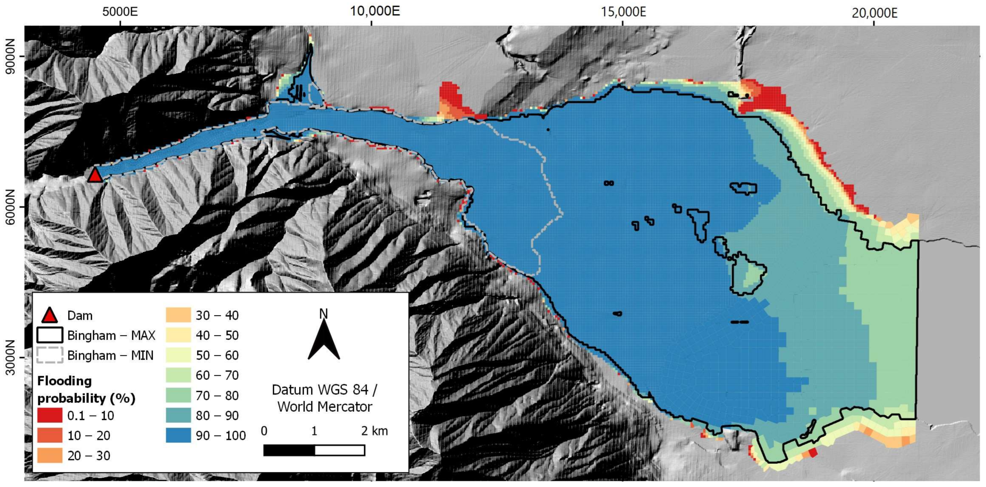
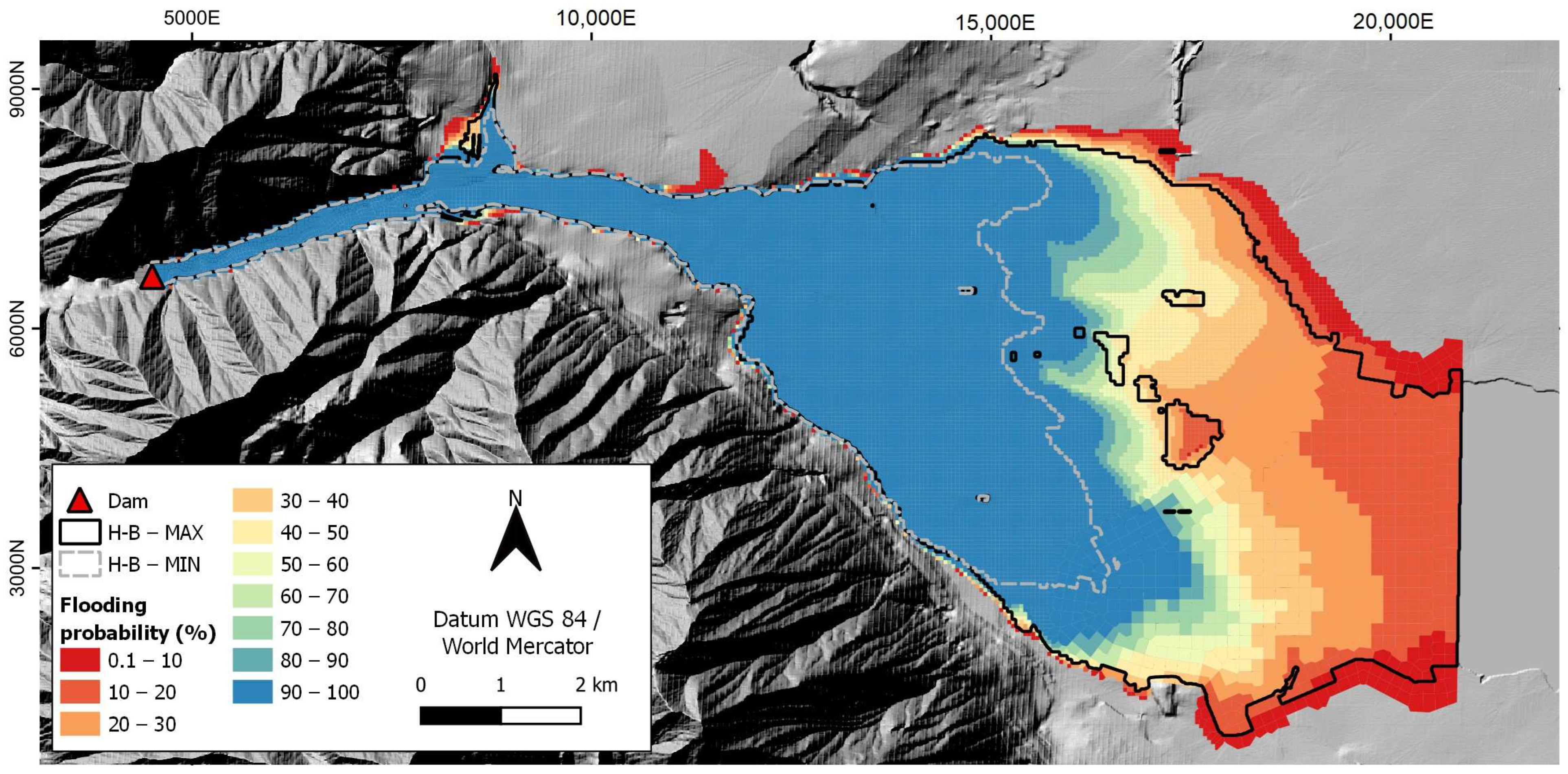
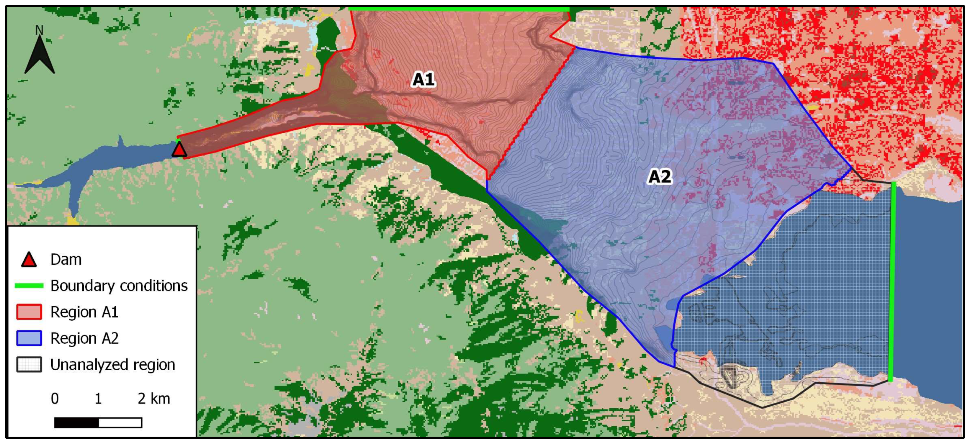
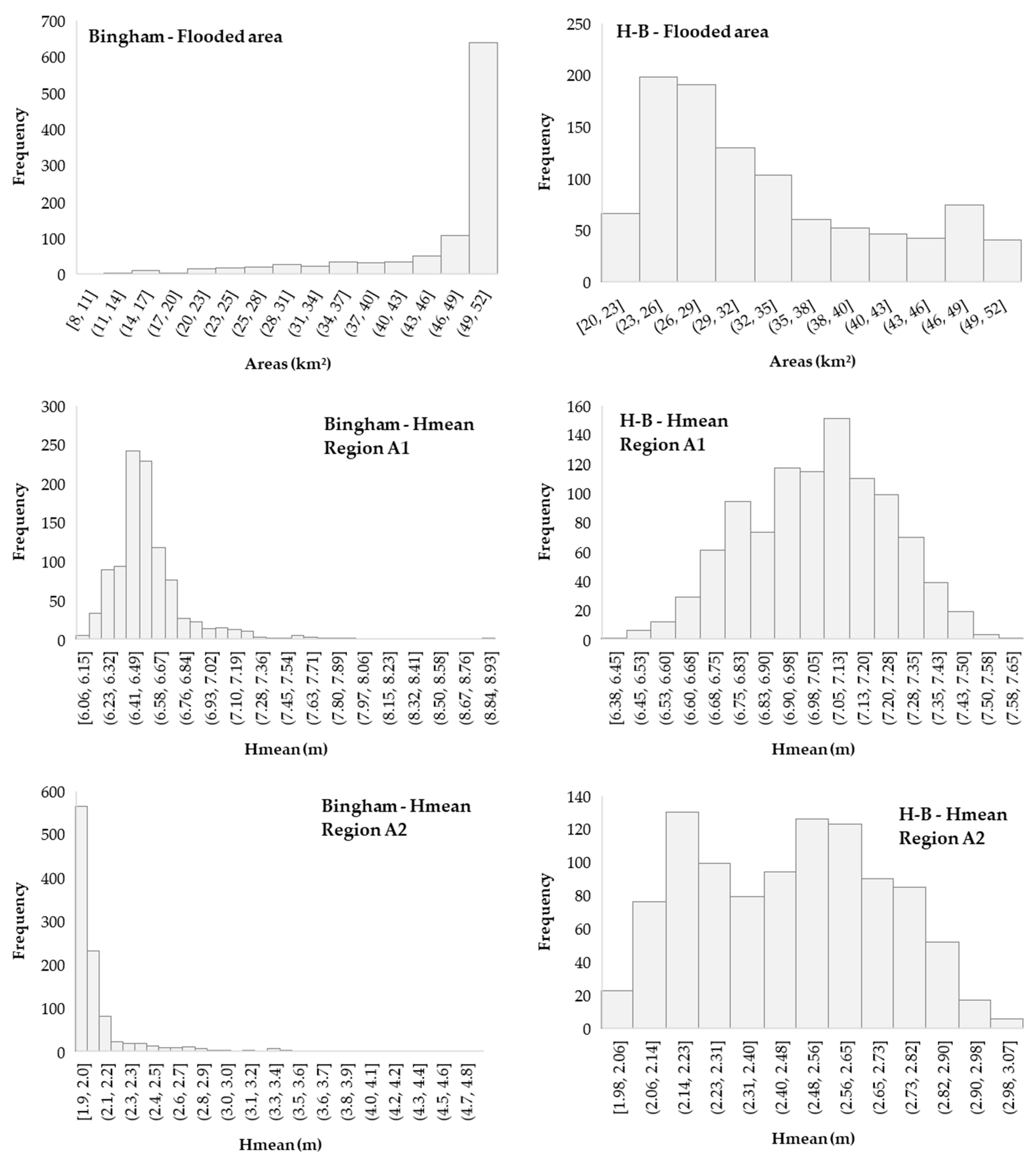
3.1. Probabilistic Maps Related to Flooded Areas

Probabilistic maps were generated by manipulating the maximum depth outcomes from each simulation and transforming these results into binary data indicating whether or not each cell area was flooded during each simulation: the value of one was assigned to flooded cells, and zero was assigned to non-flooded cells [58,61]. The flooding probabilities for each model cell were calculated using Equation (5) presented by [58].

$${\mathrm{P}}_{\mathrm{flood}}=\frac{\mathrm{NUMBER}\mathrm{OF}\mathrm{SCENARIOS}\mathrm{WITH}\mathrm{FLOODED}\mathrm{CELL}}{\mathrm{TOTAL}\mathrm{NUMBER}\mathrm{OF}\mathrm{SIMULATED}\mathrm{SCENARIOS}}$$

(5)

For both the Bingham (Figure 2) and H-B models (Figure 3), the influence of the variation of the rheological parameters on the inundation area occurs mainly in the extension of the simulated area, i.e., the downstream flood wave extent.

Within the ranges of simulated parameter values for the model, the H-B (Figure 3) presented a greater discretization of simulated areas according to the flood probabilities. Regarding the flood extent, only the maps obtained from flood probabilities between 0.1 and 20% reached the model output, and the other probability range maps indicate that the material was retained upstream. In the Bingham model (Figure 2), the flooded areas with a probability of occurrence between 50 and 80% extended to the border of the model.

Taking as a reference the area relative to the cells that were flooded in all simulations, the extent of the flooded area varied between 15.5 km (100% probability flooded) and 17.6 km (border of the simulated area) in the Bingham model. In the H-B model, the difference in flood extent was greater, about 3.2 km (from 14.3 km to 17.6 km). However, the associated probabilities were significantly lower at the border of the model for the H-B model. The Bingham model showed greater variation regarding the minimum and maximum simulated areas, with flood extents varying from 10.1 km to 17.6 km (extent difference of 7.5 km). The H-B model simulations resulted in a maximum difference in extent of 3.6 km, varying from 14.0 km to 17.6 km.

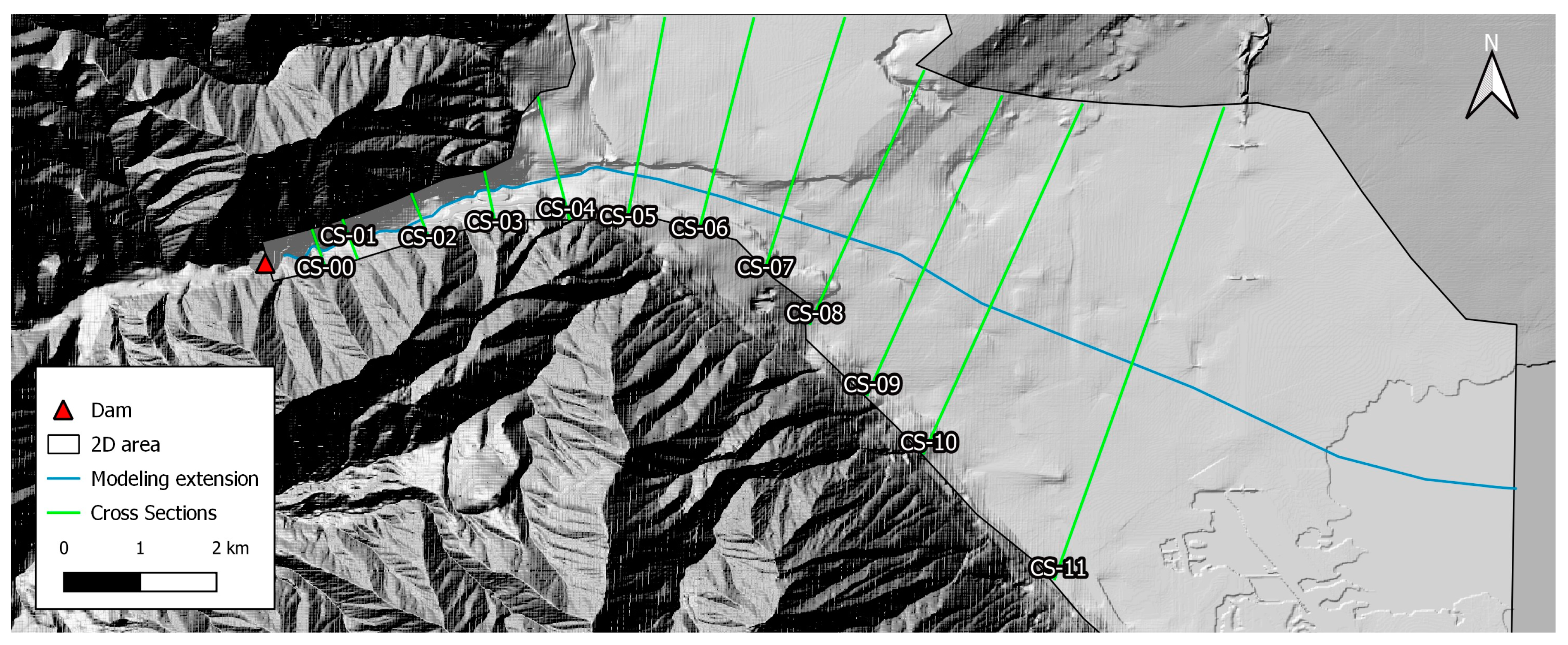
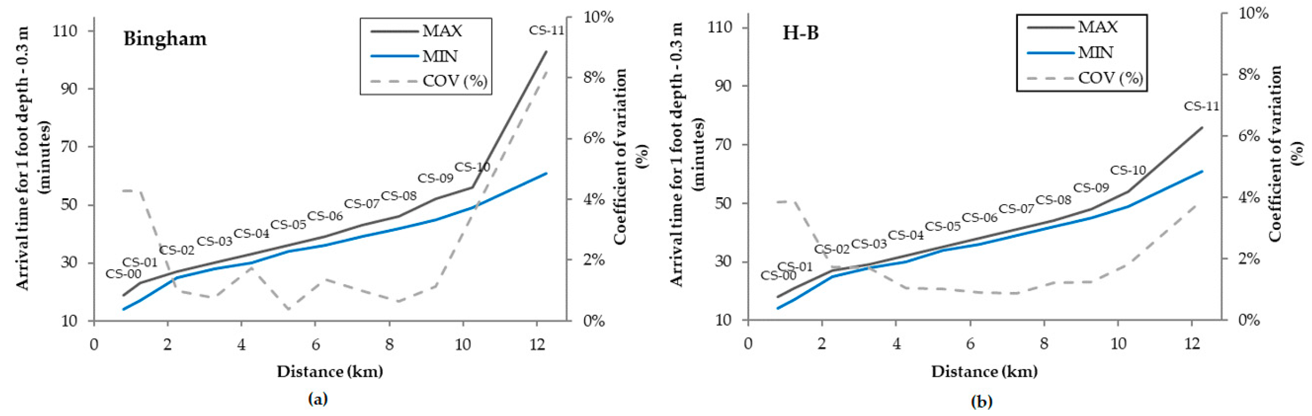
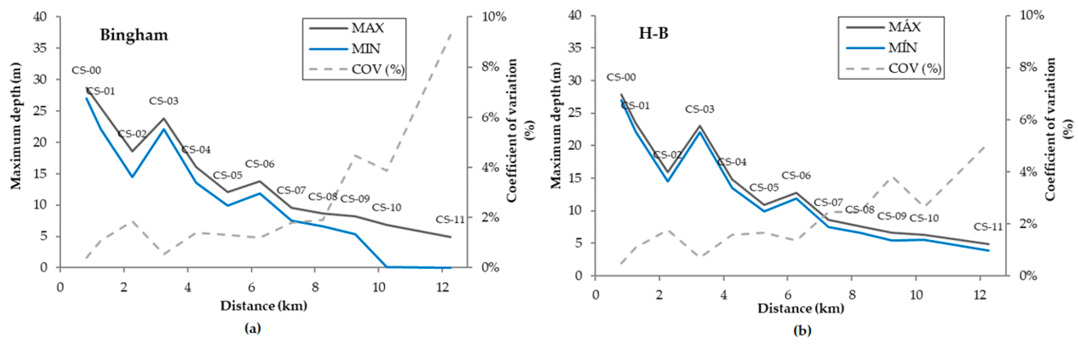
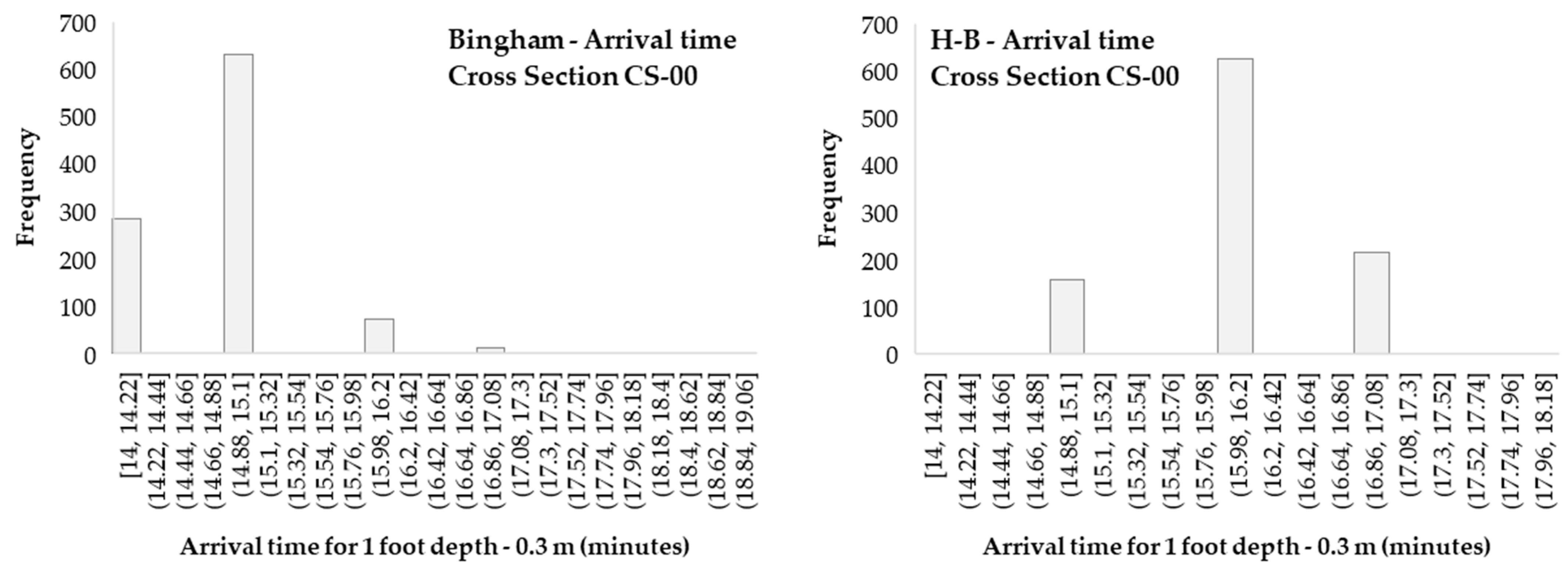
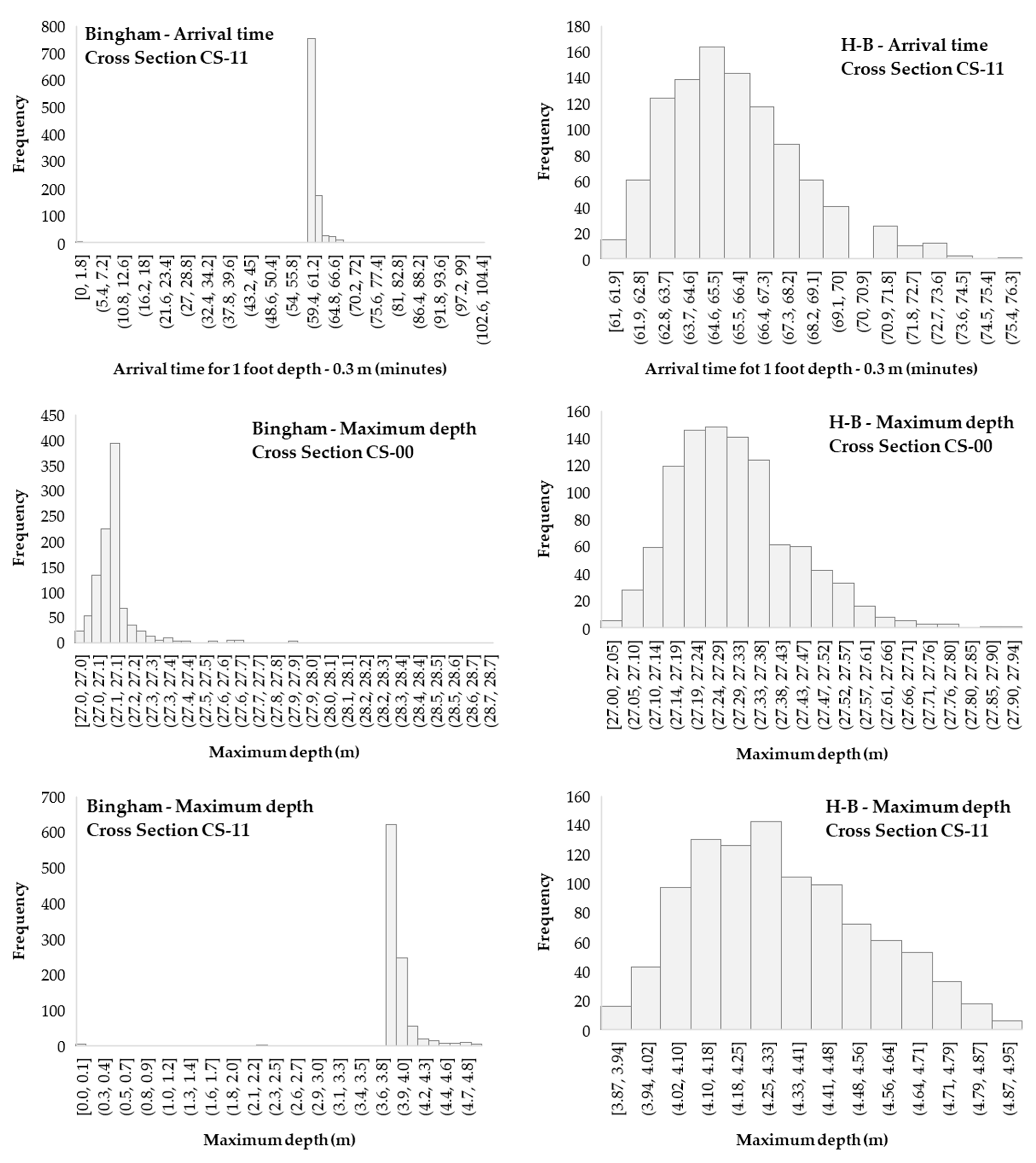
3.2. Arrival Times and Maximum Depth Variation along the Valley

To understand the impact on the dynamics of the flood event along the valley, 12 cross-sections (CS) were used for extracting and analyzing the simulation results (Figure 4): CS-00 to CS-10 (1 km of distance from each section) and CS-11, located 2 km from CS-10.

The arrival time was calculated for each CS, considering the time from the beginning of the event to the moment the depth of 0.3 m (1 foot) is reached, following the standard approach in [65]. The results presented include the maximum and minimum values and the coefficient of variation (COV %) of the arrival times comparing the 1000 simulations for both rheological models at the 11 cross-sections (Figure 5).

In general, arrival times varied between 2 and 7 min in the Bingham simulations, except for the last section, where a range of 42 min (variation from minimum to maximum values) was observed. For H-B, we observed arrival times varying from 1 to 5 min in the simulations for CS-01 to CS-10. For the last section (CS-11), a range of 15 min was observed.

For the Bingham model (Figure 5a), the greatest variation (8.2%) occurred in the last section of the model (CS-11), where the wave arrival time for the 0.3 m depth varied between 61 and 103 min; the smallest variation occurred in section CS-05 (between 34 and 36 min) with a COV equal to 0.4%. The CS-05 is located at the transition between the V-shaped valley and the flat-floored valley. In the H-B model (Figure 5b), the largest variation (3.91%) also occurred in the downstream section CS-11, where the wave arrival time for the 0.3 m depth varied between 61 and 76 min; the smallest variation occurred in section CS-07 (0.88%), which is located in the transition region between the embedded shaped valley and the flat-floored area, similar to what was observed in the Bingham model.

Regarding the depth variations simulated with the Bingham model, it can be seen that between sections CS-00 and CS-09, the maximum depths varied from a minimum of 1.8 m (CS-00) to a maximum of 4.1 m (CS-02) (Figure 6a). In the downstream sections, the variations of simulated maximum depths were higher: from 0.14 m to 6.84 m and from 0 m to 4.93 m in sections CS-10 and CS-11, respectively. These higher influences in downstream areas may be related to upstream volume retention caused by rheology parameter assumptions related to smaller flow velocities for more viscous materials. The highest COV value, 9.3%, was observed in the last downstream section, CS-11, and the lowest, 0.4%, in the most upstream section, CS-00, indicating that changes in rheological parameters were more expressive in the depths further from the dam. Although the coefficients of variation obtained are less than 10%, it is observed that the variations are relevant in absolute values of maximum depth since depths above 0.3 or 0.61 m already have significant associated risks [65].

In the H-B model, the maximum depths obtained in the analysis sections experienced the greatest variation in section CS-11 (5.1%), ranging from 3.9 m to 4.9 m (Figure 6b). The least variation in simulated maximum depths occurred in section CS-00 (0.5%), from 27.0 m to 27.9 m. Overall, the variation in maximum depths in the sections was small, ranging between 0.8 m and 1.5 m from changes in the rheological parameters of the H-B model. The qualitative variation was similar when comparing the H-B model and the Bingham one regarding the effect of the distance along the valley, with increasing variations from upstream to downstream sections.

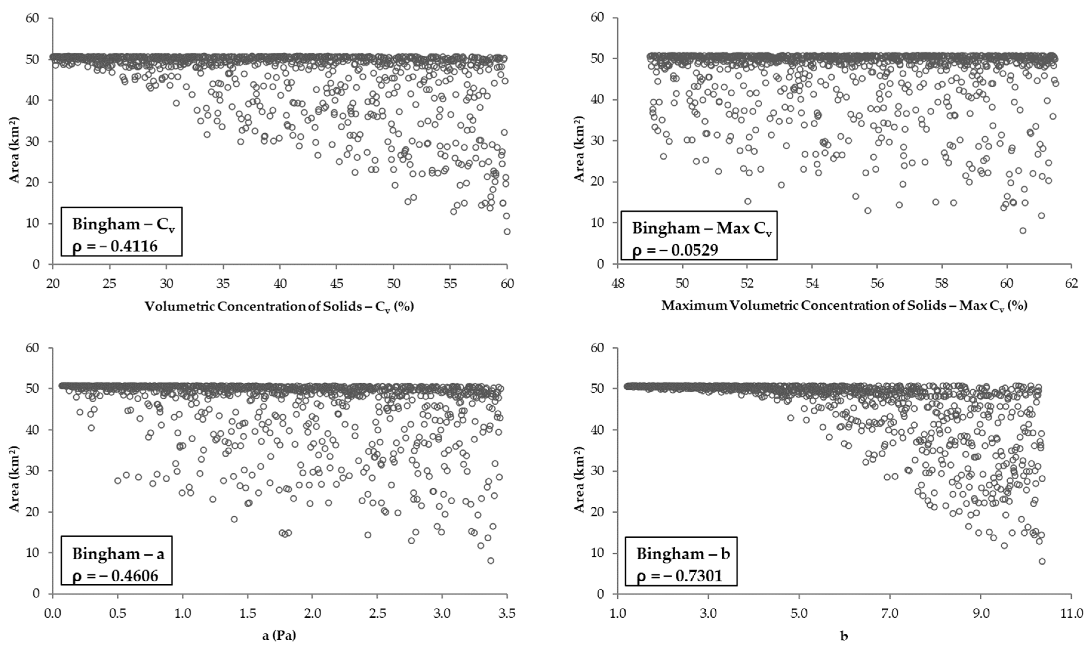
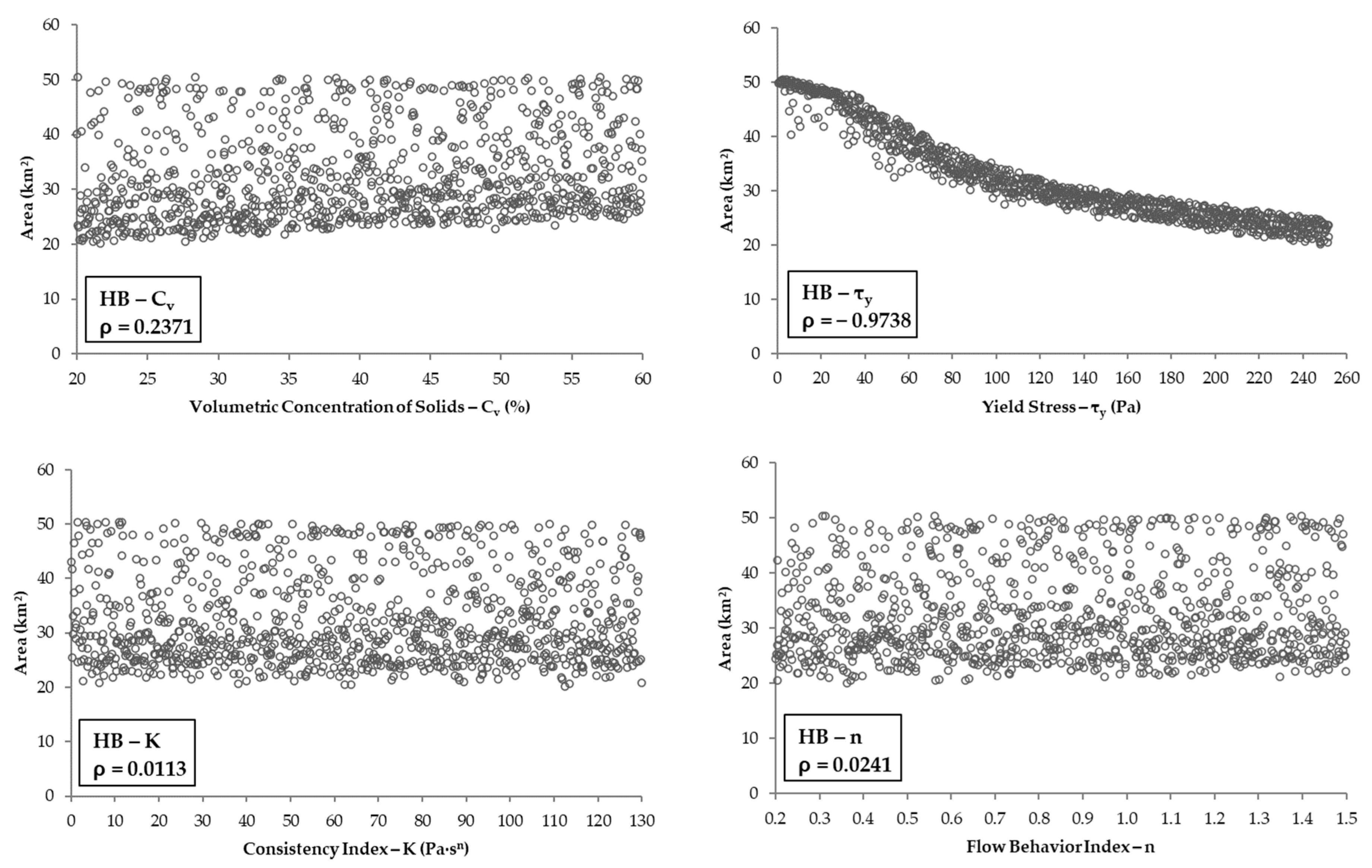
3.3. Rheological Parameters vs. Simulated Areas

With Bingham, the minimum and maximum simulated areas were 8.1 km² and 50.8 km² (Figure 7), respectively, and the area results showed a COV of 17.9%. It is observed that most simulations returned values close to the maximum one: about 68% of the simulations resulted in flooded areas within a 5% variation from the maximum simulated area (from 48.2 km² to 50.8 km²). It revealed that most sets of rheological parameters resulted in higher flooded area values. The relationships of the four parameters (C_v, Max C_v, a and b) with the flooded area indicated a tendency toward reduction in the flooded area with the increase of these input parameters, as indicated by the Spearman correlation coefficient (negative). This influence was most noticeable between the flooded area and the values of b, the exponent of the yield stress curve, which indicated the strongest correlation (ρ = −0.7301) (Figure 7). The parameters C_v and a showed moderate correlation with the flooded area, with Spearman’s correlation coefficients equal to −0.4116 and 0.4606, respectively. The parameter Max C_v showed a weak correlation with the flooded area (ρ = −0.0529). Thus, the simulations that returned smaller flooded areas are mainly related to the increase in the value of the parameter b.

In the H-B model (Figure 8), the flooded areas ranged from 20.1 km² to 50.4 km², with a coefficient of variation of 25.7%. A very strong correlation (ρ = −0.9738) is observed between the increase in yield stress (τ_y) and the reduction in flooded area (Figure 8). The variation of the parameter C_v showed a weak correlation with the flood-simulated areas (ρ = 0.2371), and the parameters K and n showed no correlation (respectively, ρ = 0.0113 and ρ = 0.0241).

Both models reached the maximum flooded area threshold of approximately 50 km². It is observed that this maximum flooded area threshold refers to physical limitations related to the terrain, roughness, runoff volume, or different sets of rheological parameters, which were defined by the modeler and considered for the different scenarios. The results showed that, in these conditions, both models were able to represent the worst-case scenario with different sets of rheologically assigned variables.

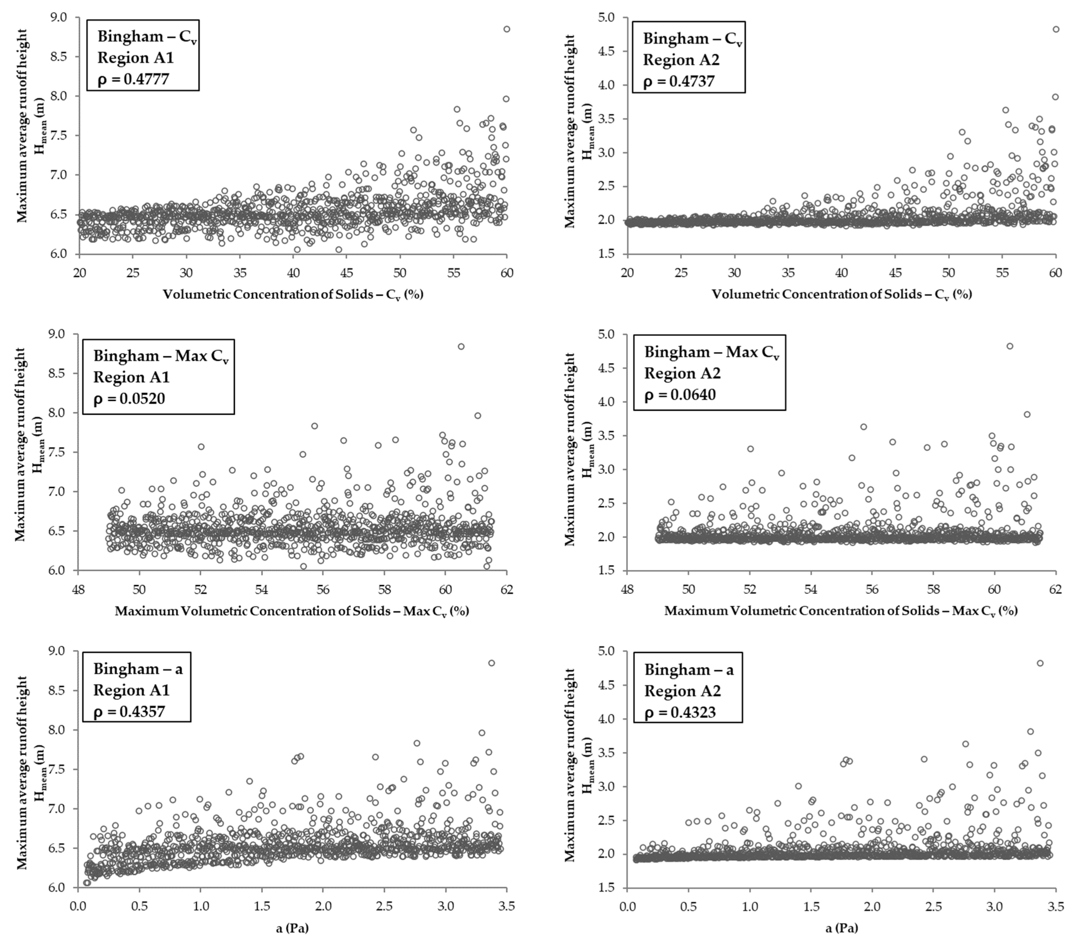
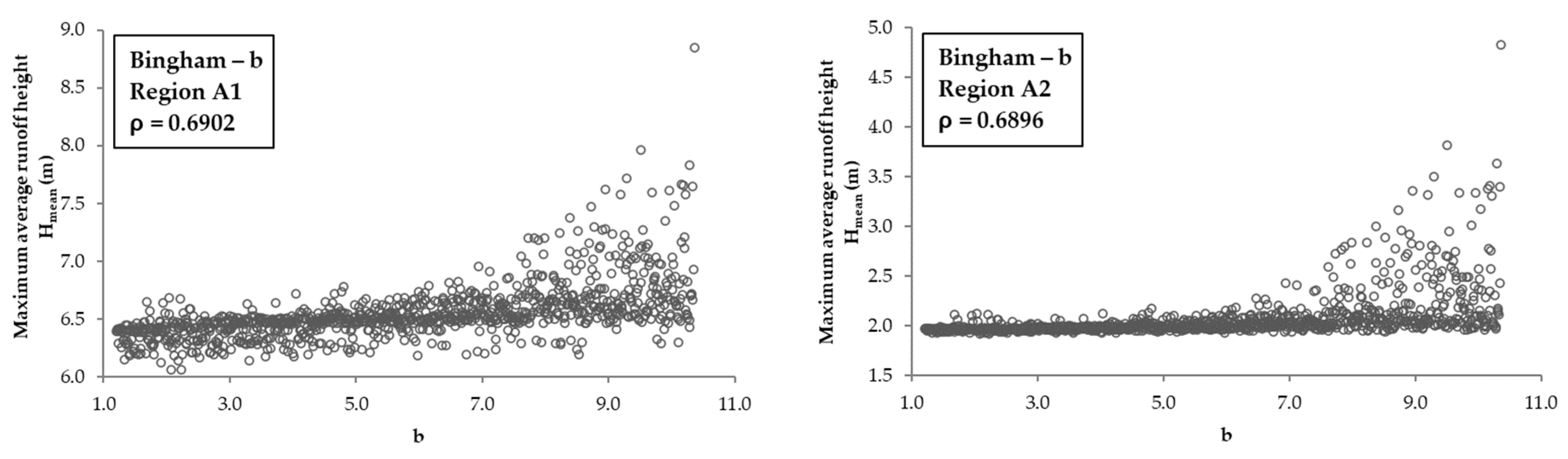
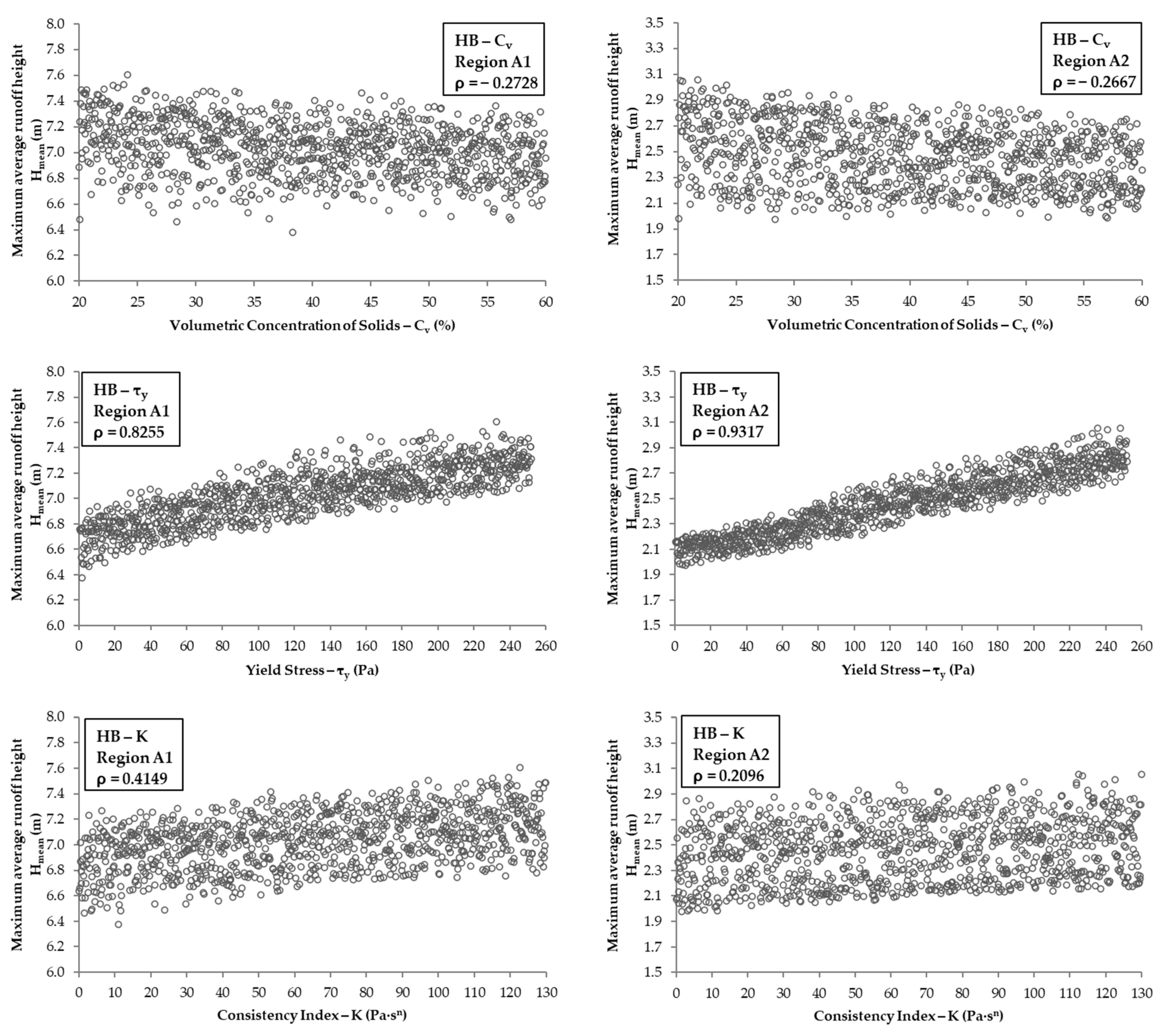
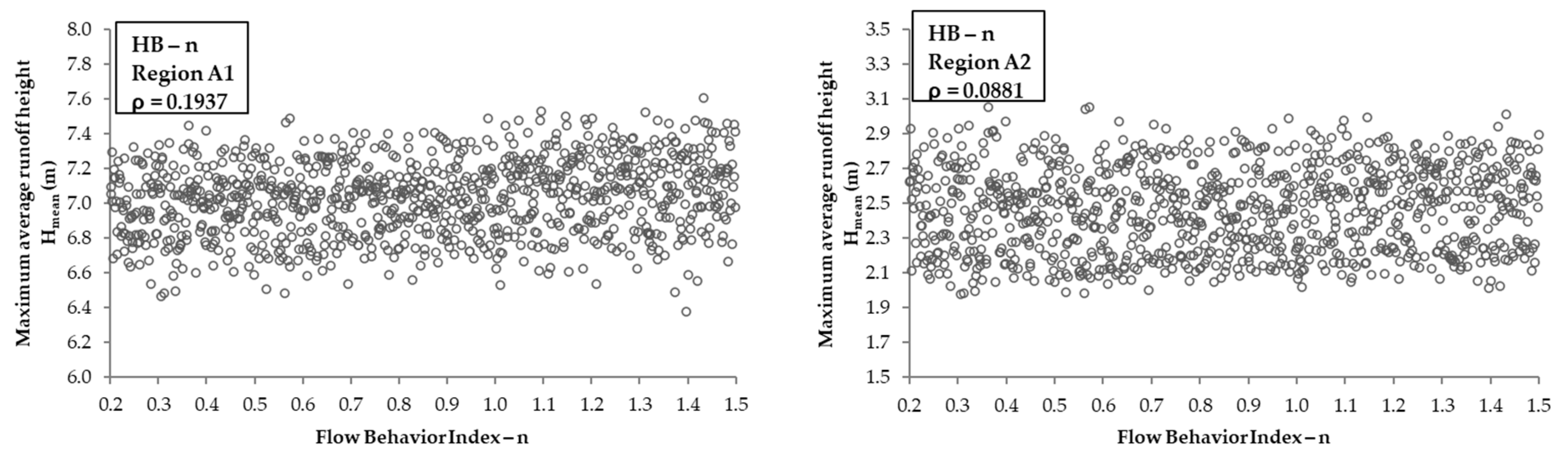
3.4. Rheological Parameters vs. H_mean

For a more general sensitivity assessment, the study area was discretized into two areas for evaluating the maximum depth variations in function of the rheological parameter determination: A1 and A2 (Figure 9).

The results of maximum depths (H_max) in the computational mesh cells for the areas of interest (A1 and A2) (Figure 9) were evaluated according to Equation (6). This equation calculates the maximum average runoff height (H_mean) for each area by summing up the maximum flow depth (H_max) in each flooded cell (H > 0) within each area and dividing the result by the total number of flooded cells (N_WC) for each area [24].

$$H_{\mathrm{mean}}={\displaystyle \sum }_{j=0}^{N_{\mathrm{WC}}}{H}_{max}\left(j\right)/N_{WC}$$

(6)

where j is the cell index; N_WC is the total number of flooded cells (h > 0); and H_max is the maximum flow depth.

The relationships between H_mean and each parameter were obtained for each area of interest for the Bingham model (Figure 10) and for the H-B model (Figure 11).

For the Bingham model, in region A1 (Figure 10), the simulated depths were greater due to the valley confinement condition immediately downstream of the dam, with average maximum depths in the cells ranging between 6.1 m and 8.8 m and a coefficient of variation equal to 3.8%. The depths reduced in the A2 region due to the spreading of the non-Newtonian fluid on the floored-shaped valley floodplain, ranging between 1.9 m and 4.8 m (COV equal to 11.8%). These results highlighted that the variation of rheological parameters has more influence on the simulated depths over the flatter region, further downstream of the dam (A2).

In region A1 (Figure 11), the resulting maximum average runoff height ranged from 6.4 m to 7.6 m and indicated a coefficient of variation of 3.0%. In the A2 region (Figure 11), the depth was reduced from upstream to downstream, ranging from 2.0 m to 3.1 m, with a COV of 9.8%. Thus, like the Bingham model, changes in the rheological parameters of the H-B model had a greater impact on the depths in the section further downstream of the simulated model, in flatter areas (A2).

For the Bingham model, in

Table 3. Spearman’s rank correction coefficients between rheological parameters and H_mean.

Results/Parameters		Bingham				Herschel H-B
		Cv	Max Cv	a	b	Cv	τy	K	n
Hmean	Region A1	0.4777	0.052	0.4357	0.6902	−0.2728	0.8255	0.4149	0.1937
	Region A2	0.4737	0.064	0.4323	0.6896	−0.2667	0.9317	0.2096	0.0881

, it is noted that Spearman’s correlation coefficient is approximately 0, i.e., an almost null correlation between maximum average runoff height and Max C_v in regions A1 and A2 (0.0520 and 0.0640, respectively). Between H_mean and b, it is verified that in both regions, A1 and A2, the larger values of b led to higher values of H_mean, with strong correlations in region A1 (0.6902) and in region A2 (0.6896).

For the H-B model (Table 3), the increase of τ_y led to the increase of H_mean, with Spearman correlation strong in region A1 (0.8255) and very strong in region A2 (0.9317). Spearman’s correlation between parameter n and depths shows a weak correlation for both regions, equal to 0.1937 and 0.0881, respectively. By the formulation of the H-B model, a more evident effect of the parameters K and n on the results was expected; therefore, the parameter ranges may have evidenced the impact of the yield stress (τ_y) on the results. Therefore, in this scenario, the parameter τ_y was the one that caused the most noticeable effect on the flooded area and the maximum average runoff height results.

4. Discussion

The Bingham and Herschel-Bulkley (H-B) models presented the same minimum arrival time simulated values along the valley (among the 1000 simulations of each model). However, when evaluating the frequency distribution of arrival times (Appendix D), the Bingham model proved to be more conservative once it presented lower values for arrival times (critical risk conditions) compared to the H-B model. With respect to the maximum arrival time values, the Bingham model indicated an extreme value in the furthest downstream section of the model. The Bingham model showed a larger coefficient of variation (variability of the data in relation to the mean) than H-B. Considering both models, the arrival times experienced greater variations further downstream of the dam, highlighting that the further downstream, the more uncertain the predictions related to this variable. Furthermore, the frequency distribution of the results in the last section shows that the Bingham model returned in most simulations arrival times close to the minimum simulated value (more conservative results), while the H-B model returned more distributed arrival times, presenting the Gamma distribution as the best fit.

Regarding the results of maximum depths along the simulated reach, the Bingham model also exhibited larger coefficients of variation in the downstream sections compared to the H-B model. The Bingham model resulted in greater depths than H-B, considering the maximum values of all simulations carried out. Nevertheless, most of the simulations with the Bingham model returned shallower depth values compared to H-B. The maximum depth results indicated the best fit to the exponential and normal distributions, in sections CS-00 and CS-11, respectively, in the Bingham model. And in the H-B model, the best fit occurred in the normal and lognormal distributions to the results of maximum depths, in sections CS-00 and CS-11. This differs from what was presented in [26], where the Gamma distribution was the best fit to the results of maximum depths and velocities in the sensitivity analysis of the MassaMov2D dynamic model to Bingham and Voellmy rheological parameters.

As for the flooded areas, the Bingham model presented a smaller coefficient of variation than the H-B model, even though the Bingham model presented a larger amplitude between the maximum and minimum values of the simulated area. The Bingham model resulted, in most simulations, in values close to the maximum value of the simulated area, once again more conservative without presenting a good fit to the probability distributions. The H-B model, on the other hand, presented more distributed flooded area values in the set of results obtained, with the best fit to the exponential distribution. For comparison purposes, the eight studies [40] that applied this same case study considering a water dam evaluated sensitivities and uncertainties related to erodibility coefficients, breach parameters, and propagation methods and models. In these studies, the simulated areas ranged from 27 km to 47 km, with a COV of 18.6%. This demonstrates how the rheological parameters have significant relevance in flood modeling since the flooded areas of the Bingham model showed COV equal to 17.9% and H-B equal to 25.7%.

The Bingham model resulted in a greater maximum average runoff height than the H-B model and showed greater coefficients of variation. The maximum average runoff height results suggest a normal and exponential distribution, respectively, in regions A1 (confined valley close to the dam) and A2 (flatter areas further from the dam) for the Bingham model. With the H-B model, in region A1, the H_mean frequency distribution showed a normal distribution of this result, and in region A2, the results were uniformly distributed.

In the Bingham model, the parameter b of the yield stress curve showed greater correlation with the results of flooded area and depths, and the parameter Max C_v was the one that showed less correlation. In the H-B model, the yield stress (τ_y) was the parameter that showed greater correlation with the variation of results, and the behavior index (n) expressed less correlation. In the results obtained by [24], it was observed that the FLO-2D model (Quadratic rheological model) is mainly sensitive to the parameter β₁ that composes the rheological curve of the dynamic viscosity, affecting mainly the results of the simulated flow depth. The study presented in [66] indicates that the results of maximum debris flow depths were more affected by the variation of the turbulent coefficient and the friction coefficient of the Voellmy rheological model in the 2D dynamic modeling with the RAMMS v.1.3.16 (Rapid Mass Movements) software. It is noticed that different hydrodynamic models have different sensitivities, which could justify future comparative tests using different approaches from this perspective.

Finally, the H-B model proved to be more sensitive to rheological parameter changes since the results varied considerably in the 1000 simulations performed. This sensitivity was expected by the H-B model formulation due to the variation of the flow behavior index (n), as pointed out in [37], although it was not the most sensitive parameter in the actual study. However, the changes in rheological parameters caused more significant impacts on the results with the Bingham model in terms of the amplitude (extreme values) of the results obtained. In this perspective, these results may indicate agreement with the conclusions presented in [8], considering that the Bingham model may be applied as a first approximation for modeling non-Newtonian flow as it presents conservative results. For a better understanding of the probabilistic variability of the simulations, it is indeed suitable to perform simulations considering the H-B model. The present study extended this understanding to dam-break analysis, leading to the same conclusions related to arrival time simulations.

5. Conclusions and Recommendations

Following the methodology developed, it was possible to bring considerable elements of answers to the main question raised within this article: “How does the rheological variability of the stored materials impact the results of the modeling of flooding caused by mining tailings dam ruptures?”.

This article demonstrated the importance of determining rheological parameters since their variability brings relevant discrepancies in terms of simulated areas, depths, and arrival times. The Bingham model was shown to be more sensitive than the H-B model in terms of maximum and minimum values of simulated areas. Furthermore, in probabilistic terms, the Bingham model was shown to be much less sensitive, tending to represent higher simulated area values, while Herschel-Bulkley showed great variability of areas as a function of the probabilities associated with the rheology parameters. Bingham was considered, on the one hand, more uncertain since it can lead to considerably lower flooded area values and, on the other hand, more conservative since, in probabilistic terms, it tends to higher area results. Therefore, the use of this model within a deterministic scheme could bring significant uncertain results. In this context, the Herschel-Bulkley model proved to be more efficient for probabilistic analysis, presenting a smaller range of uncertainties with a better distributed probability distribution, which enables a better appreciation for risk management purposes.

This article also provided contributions related to the broad bibliographic survey carried out on the ranges of values for mining tailings rheological parameters. This literature review demonstrates the great variability of these parameters and may be valuable for establishing boundaries for sensitivity analysis in other case studies. The proposed automated methodology proved robust for the evaluation of uncertainties concerning the rheological parameters in the HEC-RAS. The evaluation considers, in probabilistic terms, the flooded areas, the maximum depths reached, and the arrival times of the flood wave. Finally, the algorithm developed in Python allows for automated estimation of uncertainty in the simulation results in probabilistic terms. It is available and can be adapted for other applications in further studies.

As suggestions and recommendations for future work, it is important to evaluate the impact of the sample space of the parameters in the evaluation of the sensitivity of hydrodynamic models. The application of global sensitivity analysis [24] is a relevant alternative, as it allows a complete and complex analysis, indicating the sensitivity as a function of different indicators. In addition, since there are several sources of uncertainty in these dam failure models, the inclusion of the variation of failure breach parameters, mobilized volumes, and Manning coefficient, together with rheological parameters, would be of great importance to understanding the significance of each parameter in the results of these models in a global analysis. This type of global uncertainty analysis may provide more robustness in the study of floods and associated risks.

Furthermore, it was stated that probabilistic methods can help in defining the rheological parameters due to the high heterogeneity of the material as well as quantifying the uncertainty in the risk assessment results, which is critical to assisting planning and decision-making in more comprehensive risk analyses. Consequently, the use of this probabilistic approach in real case studies could be an interesting direction for future studies searching for a better understanding and validation of different methods.

References

1. Davies, M.P. Tailings Impoundment Failures: Are Geotechnical Engineers Listening? Geotech. News 2002, 20, 31–36. [Google Scholar]
2. Robertson, P.K.; de Melo, L.; Williams, D.J.; Wilson, G.W. Report of the Expert Panel on the Technical Causes of the Failure of Feijão Dam I. Available online: http://www.b1technicalinvestigation.com/ (accessed on 19 February 2022).
3. Morgenstern, N.R. et al Fundão Tailings Dam Review Panel. Available online: https://pedlowski.files.wordpress.com/2016/08/fundao-finalreport.pdf (accessed on 5 February 2022).
4. Julien, P.Y. Erosion and Sedimentation; Cambridge University Press: Cambridge, UK; New York, NY, USA, 1995; ISBN 978-0-521-44237-4. [Google Scholar]
5. Mezger, T. The Rheology Handbook: For Users of Rotational and Oscillatory Rheometers. In The Rheology Handbook; Vincentz Network: Hannover, Germany, 2020; ISBN 978-3-7486-0370-2. [Google Scholar]
6. O’Brien, J.S.; Julien, P.Y. Laboratory Analysis of Mudflow Properties. J. Hydraul. Eng. 1988, 114, 877–887. [Google Scholar] [CrossRef] [Green Version]
7. Faitli, J.; Gombkötő, I. Some Technical Aspects of the Rheological Properties of High Concentration Fine Suspensions to Avoid Environmental Disasters. J. Environ. Eng. Landsc. Manag. 2015, 23, 129–137. [Google Scholar] [CrossRef]
8. Jeong, S.-W. Shear Rate-Dependent Rheological Properties of Mine Tailings: Determination of Dynamic and Static Yield Stresses. Appl. Sci. 2019, 9, 4744. [Google Scholar] [CrossRef] [Green Version]
9. Zengeni, B.T. Bingham Yield Stress and Bingham Plastic Viscosity of Homogeneous Non-Newtonian Slurries. Ph.D. Thesis, Cape Peninsula University of Technology, Cape Town, South Africa, 2016. [Google Scholar]
10. Wang, X.; Wei, Z.; Li, Q.; Chen, Y. Experimental Research on the Rheological Properties of Tailings and Its Effect Factors. Environ. Sci. Pollut. Res. 2018, 25, 35738–35747. [Google Scholar] [CrossRef]
11. Jeyapalan, J.K.; Duncan, J.M.; Seed, H.B. Investigation of Flow Failures of Tailings Dams. J. Geotech. Eng. 1983, 109, 172–189. [Google Scholar] [CrossRef]
12. Yu, D.; Tang, L.; Chen, C. Three-Dimensional Numerical Simulation of Mud Flow from a Tailing Dam Failure across Complex Terrain. Nat. Hazards Earth Syst. Sci. 2020, 20, 727–741. [Google Scholar] [CrossRef] [Green Version]
13. Yang, S.-H.; Pan, Y.-W.; Dong, J.-J.; Yeh, K.-C.; Liao, J.-J. A Systematic Approach for the Assessment of Flooding Hazard and Risk Associated with a Landslide Dam. Nat Hazards 2013, 65, 41–62. [Google Scholar] [CrossRef]
14. O’ Brien, J.S.; Julien, P.Y. Physical Properties and Mechanics of Hyperconcentrated Sediment Flows; Bowles, D.D., Ed.; Delineation of Landslide, Flash Flood, and Debris-Flow Hazards in Utah; Utah Water Research Laboratory: Logan, UT, USA, 1985; pp. 260–279. [Google Scholar]
15. D’Agostino, V.; Tecca, P.R. Some Considerations On The Application Of The FLO-2D Model For Debris Flow Hazard Assessment. In Monitoring, Simulation, Prevention and Remediation of Dense and Debris Flows; WIT Press: The New Forest, UK, 2006; Volume 90, pp. 159–170. [Google Scholar]
16. Naef, D.; Rickenmann, D.; Rutschmann, P.; McArdell, B.W. Comparison of Flow Resistance Relations for Debris Flows Using a One-Dimensional Finite Element Simulation Model. Nat. Hazards Earth Syst. Sci. 2006, 6, 155–165. [Google Scholar] [CrossRef] [Green Version]
17. Sosio, R.; Crosta, G.; Frattini, P. Field Observations, Rheologucal Testing and Numerical Modeling of a Debris-Flow Event. Earth Surf. Process. Landf. 2007, 32, 290–306. [Google Scholar] [CrossRef]
18. Rickenmann, D.; Laigle, D.; McArdell, B.W.; Hübl, J. Comparison of 2D Debris-Flow Simulation Models with Field Events. Comput Geosci 2006, 10, 241–264. [Google Scholar] [CrossRef] [Green Version]
19. Cesca, M.; D’Agostino, V. Comparison between FLO-2D and RAMMS in Debris-Flow Modelling: A Case Study in the Dolomites. In Monitoring, Simulation, Prevention and Remediation of Dense Debris Flows II; WIT Press: The New Forest, UK, 2008; Volume 60, pp. 197–206. ISBN 978-1-84564-118-4. [Google Scholar]
20. Lin, J.-Y.; Yang, M.-D.; Lin, B.-R.; Lin, P.-S. Risk Assessment of Debris Flows in Songhe Stream, Taiwan. Eng. Geol. 2011, 123, 100–112. [Google Scholar] [CrossRef]
21. Hungr, O. A Model for the Runout Analysis of Rapid Flow Slides, Debris Flows, and Avalanches. Can. Geotech. J. 1995, 32, 610–623. [Google Scholar] [CrossRef]
22. Arattano, M.; Franzi, L.; Marchi, L. Influence of Rheology on Debris-Flow Simulation. Nat. Hazards Earth Syst. Sci. 2006, 6, 519–528. [Google Scholar] [CrossRef]
23. Coussot, P.; Meunier, M. Recognition, Classification and Mechanical Description of Debris Flows. Earth-Sci. Rev. 1996, 40, 209–227. [Google Scholar] [CrossRef]
24. Zegers, G.; Mendoza, P.A.; Garces, A.; Montserrat, S. Sensitivity and Identifiability of Rheological Parameters in Debris Flow Modeling. Nat. Hazards Earth Syst. Sci. 2020, 20, 1919–1930. [Google Scholar] [CrossRef]
25. Iaccarino, G. Quantification of Uncertainty in Flow Simulations Using Probabilistic Methods. In Proceedings of the Non-Equilibrium Gas Dynamics from Physical Models to Hypersonic Flights, Rhode St. Genèse, Belgium, 8 September 2008. [Google Scholar]
26. Cepeda, J.; Quan Luna, B.; Nadim, F. Assessment of Landslide Run-out by Monte Carlo Simulations. In Proceedings of the Landslides, Risk & Reliability, Paris, France, 2 September 2013; pp. 2157–2160. [Google Scholar]
27. Contreras, S.; Castillo, C.; Olivera-Nappa, Á.; Townley, B.; Ihle, C.F. A New Statistically-Based Methodology for Variability Assessment of Rheological Parameters in Mineral Processing. Miner. Eng. 2020, 156, 106494. [Google Scholar] [CrossRef]
28. Kameda, J.; Okamoto, A. 1-D Inversion Analysis of a Shallow Landslide Triggered by the 2018 Eastern Iburi Earthquake in Hokkaido, Japan. Earth Planets Space 2021, 73, 116. [Google Scholar] [CrossRef]
29. Stowe, J.; Farrell, I.; Wingeard, E. Tailings Transport System Design Using Probabilistic Methods. Min. Metall. Explor. 2021, 38, 1289–1296. [Google Scholar] [CrossRef]
30. De La Rosa, Á.; Ruiz, G.; Castillo, E.; Moreno, R. Calculation of Dynamic Viscosity in Concentrated Cementitious Suspensions: Probabilistic Approximation and Bayesian Analysis. Materials 2021, 14, 1971. [Google Scholar] [CrossRef]
31. Quan Luna, B.; Blahut, J.; van Westen, C.J.; Sterlacchini, S.; van Asch, T.W.J.; Akbas, S.O. The Application of Numerical Debris Flow Modelling for the Generation of Physical Vulnerability Curves. Nat. Hazards Earth Syst. Sci. 2011, 11, 2047–2060. [Google Scholar] [CrossRef] [Green Version]
32. Wu, Y.-H.; Liu, K.-F.; Chen, Y.-C. Comparison between FLO-2D and Debris-2D on the Application of Assessment of Granular Debris Flow Hazards with Case Study. J. Mt. Sci. 2013, 10, 293–304. [Google Scholar] [CrossRef]
33. Pasculli, A.; Cinosi, J.; Turconi, L.; Sciarra, N. Learning Case Study of a Shallow-Water Model to Assess an Early-Warning System for Fast Alpine Muddy-Debris-Flow. Water 2021, 13, 750. [Google Scholar] [CrossRef]
34. Fallas Salazar, S.; Rojas González, A.M. Evaluation of Debris Flows for Flood Plain Estimation in a Small Ungauged Tropical Watershed for Hurricane Otto. Hydrology 2021, 8, 122. [Google Scholar] [CrossRef]
35. Bingham, E.C. Fluidity and Plasticity.; McGraw-Hill: New York, NY, USA, 1922. [Google Scholar]
36. Herschel, W.H.; Bulkley, R. Konsistenzmessungen von Gummi-Benzollösungen. Kolloid-Z. 1926, 39, 291–300. [Google Scholar] [CrossRef]
37. Ligier, P.-L. Implementation of Non-Newtonian Rheological Models in TELEMAC-2D. In Proceedings of the 2020 TELEMAC-MASCARET, Online, 15 October 2020; pp. 14–25. [Google Scholar]
38. Lumbroso, D.; Davison, M.; Body, R.; Petkovšek, G. Modelling the Brumadinho Tailings Dam Failure, the Subsequent Loss of Life and How It Could Have Been Reduced. Nat. Hazards Earth Syst. Sci. 2021, 21, 21–37. [Google Scholar] [CrossRef]
39. Da Silva, A.; Eleutério, J. Effectiveness of Dam-Breach Flood Alert in Mitigating Life-Losses—A Spatiotemporal Sectorisation Analysis in a High-Density Urban Area in Brazil. Water, 2023; under review. [Google Scholar]
40. Zenz, G.; Goldgruber, M. ICOLD Proceeding, 12th International Benchmark Workshop on Numerical Analysis of Dams. In Proceedings of the ICOLD Proceedings, Gerald Zenz and Markus Goldgruber, Graz, Austria, 2 October 2013; Volume 12, p. 210. [Google Scholar]
41. Waele, A. Viscometry and Plastometry; Oil and Colour Chemists’ Association: Manchester, UK, 1923. [Google Scholar]
42. Ostwald, W. Ueber die Geschwindigkeitsfunktion der Viskosität disperser Systeme. II. Kolloid-Z. 1925, 36, 157–167. [Google Scholar] [CrossRef]
43. Qian, N.; Wan, Z. A Critical Review of the Research on the Hyperconcentrated Flow in China; International Research and Training Centre on Erosion and Sedimentation: Beijing, China, 1986. [Google Scholar]
44. de Ferreira, F.O. Abordagem Matemática de Roll Waves em Escoamentos Hiperconcentrados Com Superfície Livre. Mater’s Thesis, Universidade Estadual Paulista, Faculdade de Engenharia de Ilha Solteira, Ilha Solteira, Brazil, 2007. [Google Scholar]
45. Tarcha, B.A. Desafios na Medição da Tensão Limite de Escoamento de óleos Parafínicos. Mater’s Thesis, Universidade Federal do Espírito Santo, Centro Tecnológico, Vitória, Espírito Santo, Brazil, 2014. [Google Scholar]
46. USACE (U. S. Army Corps of Engineers) HEC-RAS Mud and Debris Flow: Non-Newtonian User’s Manual. Available online: https://www.hec.usace.army.mil/confluence/rasdocs/rasmuddebris (accessed on 5 June 2022).
47. Fitton, T.G.; Seddon, K.D. Relating Atterberg Limits to Rheology. In Proceedings of the Paste 2012, Australian Centre for Geomechanics, Perth, Australia, 16 April 2012; pp. 273–284. [Google Scholar]
48. Ribeiro, V.Q.F. Proposta de Metodologia para Avaliação do Efeito de Rupturas de Estruturas de Contenção de Rejeitos. Master’s Thesis, Universidade Federal de Minas Gerais, Belo Horizonte, Brazil, 2015. [Google Scholar]
49. Machado, N.C. Retroanálise da propagação decorrente da ruptura da barragem do fundão com diferentes modelos numéricos e hipóteses de simulação. Master’s Thesis, Universidade Federal de Minas Gerais, Belo Horizonte, Brazil, 2017. [Google Scholar]
50. Gitari, W.M.; Thobakgale, R.; Akinyemi, S.A. Mobility and Attenuation Dynamics of Potentially Toxic Chemical Species at an Abandoned Copper Mine Tailings Dump. Minerals 2018, 8, 64. [Google Scholar] [CrossRef] [Green Version]
51. Mahmood, A.A.; Elektorowicz, M. An Investigation of the Porosity Dependent Strength and Leachability of Mine Tailings Matrices Containing Heavy Metals. Cogent Environ. Sci. 2020, 6, 1743626. [Google Scholar] [CrossRef]
52. Gibson, S.; Moura, L.Z.; Ackerman, C.; Ortman, N.; Amorim, R.; Floyd, I.; Eom, M.; Creech, C.; Sánchez, A. Prototype Scale Evaluation of Non-Newtonian Algorithms in HEC-RAS: Mud and Debris Flow Case Studies of Santa Barbara and Brumadinho. Geosciences 2022, 12, 134. [Google Scholar] [CrossRef]
53. Bagnold, R.A. Experiments on a Gravity-Free Dispersion of Large Solid Spheres in a Newtonian Fluid under Shear. Proc. R. Soc. Lond. A 1954, 225, 49–63. [Google Scholar] [CrossRef]
54. Rickenmann, D. Hyperconcentrated Flow and Sediment Transport at Steep Slopes. J. Hydraul. Eng. 1991, 117, 1419–1439. [Google Scholar] [CrossRef]
55. Olsson, A.; Sandberg, G.; Dahlblom, O. On Latin Hypercube Sampling for Structural Reliability Analysis. Struct. Saf. 2003, 25, 47–68. [Google Scholar] [CrossRef]
56. McKay, M.D.; Beckman, R.J.; Conover, W.J. A Comparison of Three Methods for Selecting Values of Input Variables in the Analysis of Output from a Computer Code. Technometrics 1979, 21, 239–245. [Google Scholar] [CrossRef]
57. Pirouz, B.; Javadi, S.; Seddon, K. Thickener Performance Variability: Underflow Solids Concentration and Flowrate. In Proceedings of the Paste 2017, University of Science and Technology Beijing, Beijing, China, 16 June 2017; pp. 29–40. [Google Scholar]
58. Bezerra, R.; Eleutério, J. A Novel Full 2D Probabilistic Hydrodynamic Approach to Model and Map Floods from Dam Failures Considering Breach Parameters Uncertainty. Water, 2023; under review. [Google Scholar]
59. Goodell, M.C.R. Breaking the HEC-RAS Code: A User’s Guide to Automating HEC-RAS, 1st ed.; H2ls: Portland, OR, USA, 2014; ISBN 978-0-9908918-0-2. [Google Scholar]
60. Dysarz, T. Application of Python Scripting Techniques for Control and Automation of HEC-RAS Simulations. Water 2018, 10, 1382. [Google Scholar] [CrossRef] [Green Version]
61. Papaioannou, G.; Vasiliades, L.; Loukas, A.; Aronica, G.T. Probabilistic Flood Inundation Mapping at Ungauged Streams Due to Roughness Coefficient Uncertainty in Hydraulic Modelling. Adv. Geosci. 2017, 44, 23–34. [Google Scholar] [CrossRef] [Green Version]
62. Hamouda, T. Impact of Micro-Topography and Bathymetry Modification on Inundation Modelling with Different Magnitudes Based on SRTM Data. Master’s Thesis, UNESCO-IHE Institute for Water Education, Delft, The Netherlands, 2018. [Google Scholar]
63. Da Silva, A.Â.C.L.; Eleutério, J.C. Identifying and Testing the Probability Distribution of Earthfill Dam Breach Parameters for Probabilistic Dam Breach Modeling. J. Flood Risk Manag. 2023, e12900. [Google Scholar] [CrossRef]
64. Froehlich, D. Empirical Model of Embankment Dam Breaching. In Proceedings of the River Flow 2016, St. Louis, MO, USA, 11–14 July 2016; CRC Press: Boca Raton, FL, USA, 2016; pp. 1821–1826. [Google Scholar]
65. FEMA (Federal Emergency Management Agency). Federal Guidelines for Inundation Mapping of Flood Risks Associated with Dam Incidents and Failures; FEMA: Washington, DC, USA, 2013; p. 145.
66. Hussin, H.Y. Probabilistic Run-out Modeling of a Debris Flow in Barcelonnette, France. Thesis, ITC: Faculty of Geo-Information Science and Earth Observation, Enschede, The Netherlands, 2011. Available online: http://essay.utwente.nl/84877/ (accessed on 30 July 2023).
67. Wooster, J.K.; Dusterhoff, S.R.; Cui, Y.; Sklar, L.S.; Dietrich, W.E.; Malko, M. Sediment Supply and Relative Size Distribution Effects on Fine Sediment Infiltration into Immobile Gravels. Water Resour. Res. 2008, 44. [Google Scholar] [CrossRef] [Green Version]
Figure 1. Two-dimensional model of the ICOLD case study used in the simulations with HEC-RAS.
Water 15 02866 g001
Figure 2. Probabilistic mapping of the Bingham model.
Water 15 02866 g002
Figure 3. Probabilistic map of the Herschel-Bulkley (H-B) model.
Water 15 02866 g003
Figure 4. Results analysis sections.
Water 15 02866 g004
Figure 5. Variation of arrival time along the downstream talweg for simulations using the (a) Bingham model and (b) Herschel-Bulkley (H-B) model.
Water 15 02866 g005
Figure 6. Variation of maximum depths along the downstream talweg for the (a) Bingham and (b) H-B models.
Water 15 02866 g006
Figure 7. Relationship between flooded areas and Cv, Max Cv, a, and b in 1000 simulations with the Bingham model.
Water 15 02866 g007
Figure 8. Relationship between inundated areas and Cv, τy, K, and n in 1000 simulations with the H-B model.
Water 15 02866 g008
Figure 9. Discretized areas for sensitivity evaluation.
Water 15 02866 g009
Figure 10. Relationships between maximum average runoff height (Hmean) and the parameters Cv, Max Cv, a, and b in the areas of interest, A1 and A2—Bingham Model results.
Water 15 02866 g010aWater 15 02866 g010b
Figure 11. Relationships between the maximum average runoff height (Hmean) and the parameters Cv, τy, K, and n in the areas of interest, A1 and A2—H-B model results.
Water 15 02866 g011aWater 15 02866 g011b