Article

Evaluating Urban Stream Flooding with Machine Learning, LiDAR, and 3D Modeling

by
Madeleine M. Bolick
1,*,
Christopher J. Post
1,
M. Z. Naser
2,
Farhang Forghanparast
2 and
Elena A. Mikhailova
1
1
Department of Forestry and Environmental Conservation, Clemson University, Clemson, SC 29634, USA
2
School of Civil and Environmental Engineering and Earth Sciences, Clemson University, Clemson, SC 29634, USA
*
Author to whom correspondence should be addressed.
Water 2023, 15(14), 2581; https://doi.org/10.3390/w15142581
Submission received: 16 May 2023 / Revised: 4 July 2023 / Accepted: 10 July 2023 / Published: 14 July 2023

Abstract

:
Flooding in urban streams can occur suddenly and cause major environmental and infrastructure destruction. Due to the high amounts of impervious surfaces in urban watersheds, runoff from precipitation events can cause a rapid increase in stream water levels, leading to flooding. With increasing urbanization, it is critical to understand how urban stream channels will respond to precipitation events to prevent catastrophic flooding. This study uses the Prophet time series machine learning algorithm to forecast hourly changes in water level in an urban stream, Hunnicutt Creek, Clemson, South Carolina (SC), USA. Machine learning was highly accurate in predicting changes in water level for five locations along the stream with R2 values greater than 0.9. Yet, it can be challenging to understand how these water level prediction values will translate to water volume in the stream channel. Therefore, this study collected terrestrial Light Detection and Ranging (LiDAR) data for Hunnicutt Creek to model these areas in 3D to illustrate how the predicted changes in water levels correspond to changes in water levels in the stream channel. The predicted water levels were also used to calculate upstream flood volumes to provide further context for how small changes in the water level correspond to changes in the stream channel. Overall, the methodology determined that the areas of Hunnicutt Creek with more urban impacts experience larger rises in stream levels and greater volumes of upstream water during storm events. Together, this innovative methodology combining machine learning, terrestrial LiDAR, 3D modeling, and volume calculations provides new techniques to understand flood-prone areas in urban stream environments.

1. Introduction

Urban stream flooding causes structural and property damage, and its frequency increases as urbanization and development grow [1]. Urban watersheds are characterized by having a large percentage of impervious surfaces, such as roads, parking lots, buildings, and sidewalks, that do not allow water to percolate into the soil. Instead, water flows rapidly off these impervious surfaces into the nearest waterbody source, which can cause rapid increases in water levels, leading to flooding [2]. This runoff also brings pollution into the stream channels by carrying trash, bacteria, and petroleum products from impervious surfaces into the streams, negatively impacting the stream’s water quality [3]. Climate change is predicted to cause more extreme precipitation events, resulting in more frequent and extreme flood events in urban areas [4,5].
Due to the impervious surfaces and development in urban watersheds, the hydrology of these systems differs from natural areas that have vegetation [6]. Urbanization contributes to more rapid transitions from base flow to high flow conditions during a storm, more variable streamflow levels throughout the day, increased occurrences of high-water levels, and lower frequencies of low base flows [7]. These differences in streamflow patterns and frequent changes need to be acknowledged and addressed to combat the negative impacts of urban stream flooding [8]. Therefore, new techniques need to be developed that focus on these urban streams and consider the hardened structures present in the systems, like culverts and metal pipes, that redirect stream flow or replace natural stream channel areas.
Traditional flood forecasting or flood modeling uses HEC-RAS software from the U.S. Corps of Engineers [9,10]. For example, Kolakovic et al. [11] used terrestrial LiDAR-derived stream channel models in HEC-RAS to produce hydraulic flood modeling for the Danube River in Southeast Europe. A recent study used HEC-RAS to identify flood-prone areas for different rainfall scenarios in the Prosa basin in Brazil [12]. While HEC-RAS is a useful tool for hydrology and flood modeling, it requires large amounts of input data such as stream geometry, flow data, and flow regime information [13]. Much of this stream characterization information may not be available for urban stream areas for flood risk analysis. Therefore, researchers and stream managers may need to use other flood forecasting methodologies that can utilize the available stream information. Additionally, HEC-RAS software is designed to model flood events with specific, more extreme return periods, such as 20, 50, or 100 years [13], rather than forecasting future flood events based on commonly occurring conditions at the stream location.
Water level and flood forecasting have shifted in recent years to machine learning techniques because the algorithms can predict changes in water level based on stream conditions more quickly and with less input data than HEC-RAS [14,15,16]. In machine learning, computer models are trained with water quality and water quantity variables to teach an algorithm to make predictions [16]. Machine learning is often a faster, more efficient way to forecast flooding and can produce highly accurate results with smaller amounts of input data [17]. For example, Sahoo et al. [18] used a long short-term memory recurrent neural network machine algorithm to forecast periods of low flow in the Mahanadi River basin in India. A newly developed machine learning time series algorithm, Prophet, has recently been applied to hydrology problems, such as predicting streamflow from precipitation and temperature data [19]. Machine learning has also been used to develop flood warning systems that can predict the possibility of flooding in the future based on information, such as precipitation levels [20,21,22]. These machine learning prediction techniques can be helpful for stream and risk managers to help prepare for future flooding events.
Being able to forecast water levels in urban areas is particularly important due to the greater impact of flooding on infrastructure and developments. Applying machine learning to urban stream water levels can alert managers to potential flood events, and they can take action to prevent catastrophic damage. A recent study in Fuzhou City, China used long short-term memory (LSTM) machine learning strategies to forecast river water levels using only upstream water level measurements [23]. In the Shibuya River Basin in Tokyo, researchers used a time series vector autoregressive machine learning model to predict water levels to act as an evacuation warning system [24]. This model used water level data and average rainfall data to make water level predictions twenty minutes in advance of flood events [24]. In the Dorim stream basin in Seoul, deep learning was used to forecast flooding under extreme rainfall conditions using only forecasted rainfall information [25]. These studies represent a more recent focus on the importance of studying urban areas.
In addition to machine learning, other technologies can assist researchers in understanding the flood potential of urban watersheds. LiDAR (Light Detection and Ranging) is a technique used in remote sensing where laser light is used to measure topography. LiDAR sensors measure how the light emitted from the sensor bounces off the surrounding land, which then allows the user to recreate the scanned area as a point cloud [26]. This point cloud can then be translated into digital elevation models (DEMs) that illustrate the bare earth ground elevations, digital surface models (DSMs) that represent the tops of vegetation and buildings above the ground, and 3D models [27]. LiDAR data can be collected from aerial sensors that are mounted on airplanes or helicopters, which can measure large areas of topography, but the resolution of the LiDAR data is lower for aerial sensors because there are fewer laser pulses per meter [28]. LiDAR data can also be collected using terrestrial sensors that are mounted on things like moving vehicles or backpacks [29]. Because these terrestrial LiDAR units are closer to the ground and move more slowly when collecting data, the resolution of the point clouds is higher, resulting in higher-resolution DEMs and DSMs [28,30].
Many studies have found that terrestrial LiDAR scanning provides high-resolution data that enables accurate modeling of stream channels and the surrounding riparian area that can be useful for vegetation analysis [31], sediment erosion [32], and flood analysis [33]. Higher resolution DEMs and 3D models are necessary to correctly analyze flooding and water level increases in urban streams because microtopography features influence flow paths, flow velocity, and the resulting flood intensity [34]. For example, Costabile et al. [33] used terrestrial LiDAR scanning to create 0.5 m resolution DEMs and detailed 3D models of riparian areas to create flood hazard maps for risk managers.
New methods are needed to analyze urban stream watersheds to learn how the system responds to storms and what actions can be taken to mitigate the negative impacts of rapid water level rise and flooding. This study combines the predictive power of machine learning to forecast water levels. The study then translates these values into 3D visualizations and volume calculations to understand the flood potential in an urban stream, Hunnicutt Creek, located in Clemson University’s campus in Clemson, South Carolina, USA. Machine learning predictions for water level rise are helpful warning alerts to times of increased water levels, but the forecasting alone does not provide a full picture of the flooding potential in the watershed. Therefore, this study also uses terrestrial LiDAR to gather dense point clouds to create high-resolution DEMs and 3D stream channel models and calculates changes in water volume in the upstream catchment areas. Using this high-resolution LiDAR data and DEMs, along with the water volume information, allows for a detailed analysis of stream channels and provides insights into the flooding capacity of Hunnicutt Creek by showing specifically how different water level increases correspond to water in the stream channel. This study demonstrates a new methodology to evaluate and understand flood scenarios in urban settings where water levels can rise rapidly in short time periods.

2. Materials and Methods
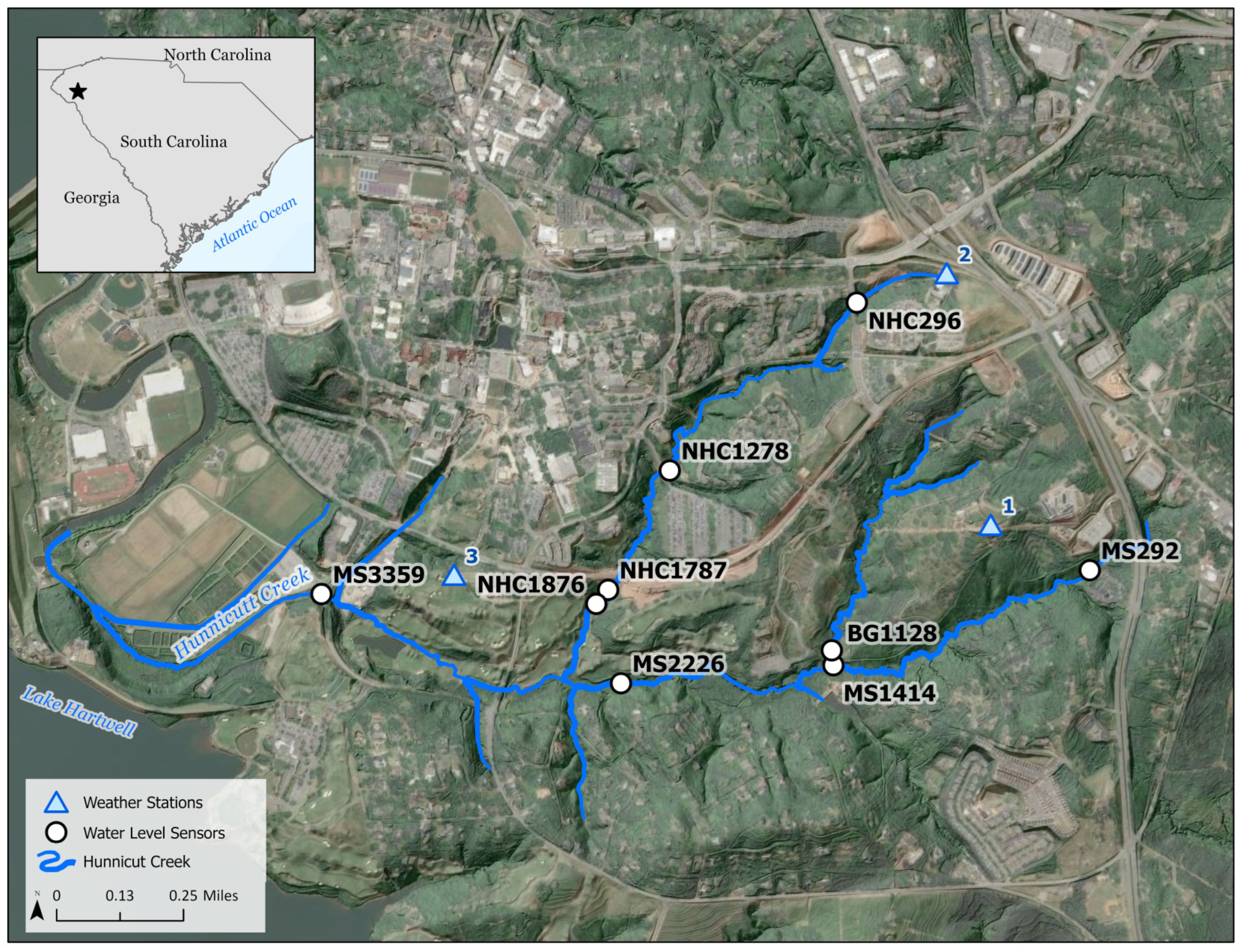
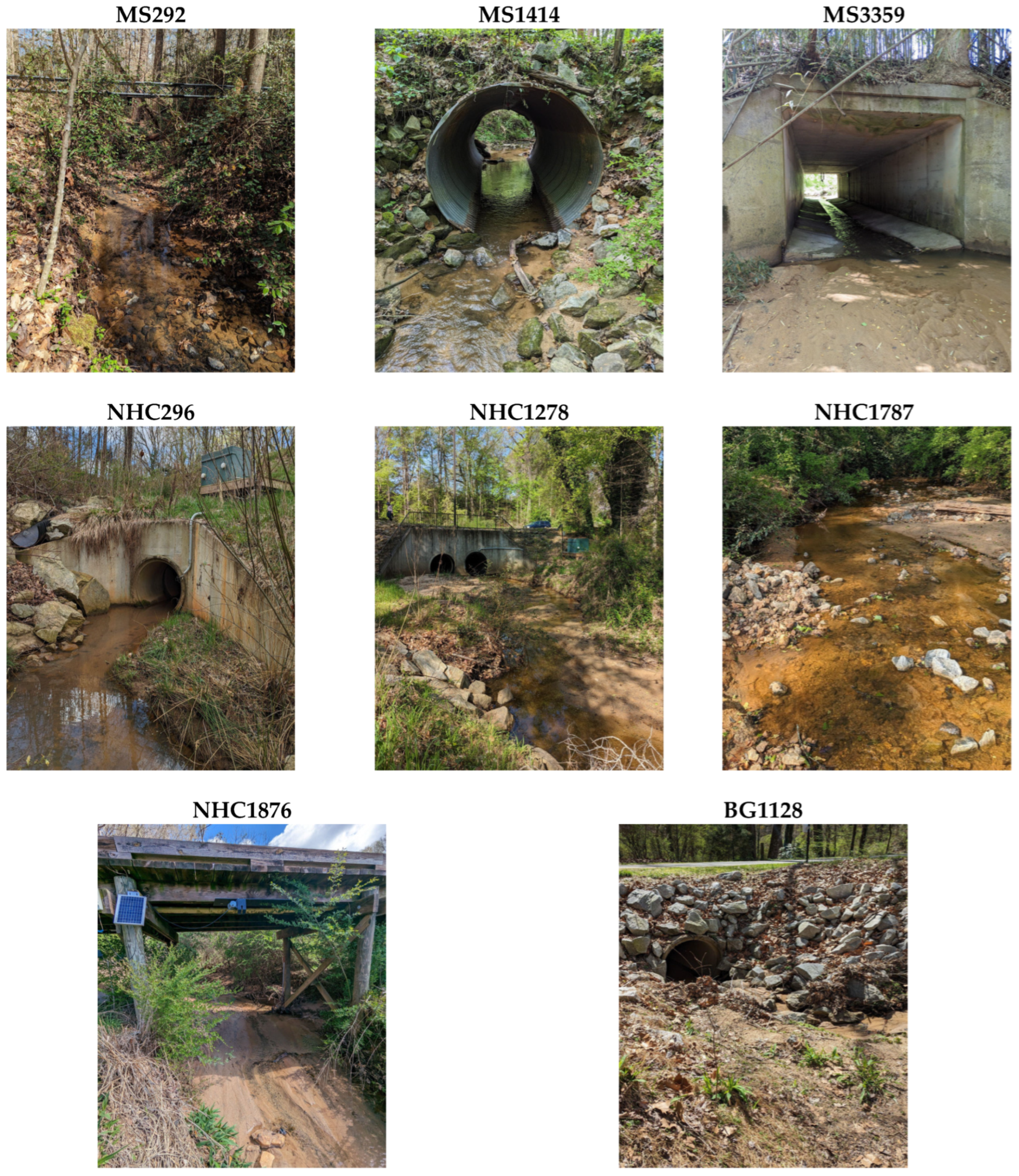
2.1. Study Area

Hunnicutt Creek is approximately a two-square-mile urban watershed in the Seneca River Watershed in Clemson, SC, United States (HUC code 03060101). The stream is 4.5 km long and begins outside of campus west of U.S. Route 76 and flows through the Clemson University campus to the west, where it ends at a U.S. Army Corps of Engineers pump station directing flow into Lake Hartwell. A recent water quality study of Hunnicutt Creek calculated the overall land cover for the watershed and found the area comprises 0.2% water, 21.6% low vegetation, such as grass and bushes, 53% tree canopy, and 25.2% impervious surfaces [35], illustrating that the watershed comprises a mix of natural and impervious areas. The study area is in Pickens County, which receives an average of 53.44 inches of rain per year, and temperatures range from 47 °F in the winter to 72 °F in the summer [36].
Hunnicutt Creek is monitored by a series of water quality and water level sensors throughout the watershed as part of the Intelligent River® project [37] at specific station locations (Figure 1). Station locations are named based on the branch of Hunnicutt Creek they are placed on. For example, the stations along the main stem of Hunnicutt Creek have a name that starts with ‘MS’, stations that are along the northern branch of Hunnicutt Creek start with ‘NHC’, and stations that are along the branch of Hunnicutt Creek that passes through the South Carolina Botanical Gardens begin with ‘BG.’ The numbers that follow the Hunnicutt Creek branch abbreviation represent how many meters the location is from the headwaters of that stream branch. For example, station NHC1278 means that the sensor is located along the northern branch of Hunnicutt Creek, 1278 m from the creek’s origin. The water level sensors in the stream measure the distance from the sensor to the water level in millimeters. They are spaced throughout the stream to understand how water levels change in different watershed areas. Some of these sensors are placed in areas of the stream with natural sandy bottoms, while others are placed in hardened structures, such as stormwater pipes, to understand how conditions may differ depending on the area of the urban stream (Figure 1).
Each station location along Hunnicutt Creek is unique due to the mix of urban and natural areas around the stream (Figure 2). Station MS292 is a natural area with undisturbed stream banks and a rocky upstream channel. Station MS1414 is located in the South Carolina Botanical Gardens inside a 70-inch metal corrugated pipe directing Hunnicutt Creek under a small land bridge. Station MS3359 is at the end of a large concrete culvert directing stream flow under a road. Station NHC296 is located downstream of a recently restored area of Hunnicutt Creek, where the floodplain was widened to accommodate rises in stream flow, allowing water to disperse in the floodplain and prevent campus flooding. This location’s (NHC296) water level sensor is inside a 42-inch reinforced concrete pipe. Station NHC1278 has the sensor inside a 60-inch reinforced concrete pipe, and the upstream area is in more natural condition. Station NHC1787 is located in a natural stream length in Hunnicutt Creek along a golf course. Stream flow upstream of this site is directed through a concrete pipe. Station NHC1876 is slightly downstream from NHC1787 and is located under a wooden bridge in the golf course. Station BG1128 is located in the Botanical Gardens inside of a 47-inch concrete pipe, and the upstream area has been reinforced with large rocks.
In addition to the water level stations, three weather stations are also placed throughout the Hunnicutt Creek watershed, numbered 1-3, and collect precipitation (mm), air temperature (°C), and relative humidity (%) measurements every 5–6 min.
During storm events, some rainwater can permeate the areas of vegetation and grass, but the water that falls on impervious surfaces is either redirected via stormwater infrastructure to Hunnicutt Creek or becomes surface runoff that ultimately reaches Hunnicutt Creek. During large precipitation events, Hunnicutt Creek’s water level can quickly rise, overflow its banks, and flood onto roads (Figure 3). Flooding in the watershed has led to dangerous driving conditions and sinkholes.

2.2. Machine Learning

2.2.1. Data Preparation

The data from the Intelligent River® sensors and the weather station data were downloaded from the program’s private online database for the available data during 2022. Depending on the site location, different water quality, quantity, or weather information was available (Table 1). Station locations MS1414, MS3359, NHC296, NHC1286, and NHC1876 were used for the machine learning analysis. Since the water level sensors measure the sensor location to the water level, these values were converted to a change in water level value by finding the largest distance reading (which corresponds to the lowest water level or base flow level) and subtracting each row’s distance measurement from this number. The resulting number indicates how much the water level increases in millimeters from base flow conditions.
The time at which each measurement is recorded also varies for each station, and each sensor takes measurements typically every 11–13 min. The data were converted into 1 h intervals to allow consistency across all sites. For instance, the average of turbidity, dissolved oxygen, relative humidity, air temperature, water temperature, and change in water level were calculated in 1 h increments. If the sensor recorded multiple readings for one hour, the average of the readings was taken. Precipitation was treated differently, and these values were summed to obtain the total amount of precipitation during each 1 h period. This is because it is important to know the total precipitation amount instead of an average precipitation amount, which would not accurately depict the storm event.
Each 1 h interval dataset was evaluated for outliers, which were removed. All missing values (NAs) for changes in water level were also removed. The change in water level serves as the dependent variable, so the log of this variable was taken to minimize the large fluctuations in this value to improve machine learning performance.
The water quality and quantity 1 h interval datasets were combined with the closet weather station dataset by matching the date and time of the 1 h increments. The weather data at each station included the variables air temperature (°C), precipitation (mm), and relative humidity (%). Finally, all rows with no precipitation were removed to focus on the changes in water level during storm events.

2.2.2. Prophet Algorithm

The time series machine learning algorithm, Prophet [38], was used to predict the change in water level in Hunnicutt Creek at the different station locations. Prophet is an open-source custom time series regression algorithm designed originally to forecast a variety of Facebook data, such as platform usage and growth, and it can be used in both Python and R [38]. The algorithm was designed to be flexible to work with a wide variety of data types and to be simple to implement with easy-to-understand parameters [38]. Prophet uses a time series model [39] and adds trend, seasonality, and holidays to the equation described in Equation (1).
y t = g t + s t + h t + t
The trend function g(t) models value changes in the input time series data, s(t) is the seasonal period changes in the data, h(t) is the effect holidays may have on the data over one or more days, and ∈(t) is the error term that captures changes the model does not account for [39]. The holiday effect was not utilized when applying this equation to this study’s water level data change.
While originally designed for business time series data with yearly, seasonal, monthly, daily, or hourly trends, a variety of recent studies have explored the Prophet algorithm’s potential with hydro-environmental time series data. For example, Prophet outperformed two other algorithms, ARIMA, and ThymeBoost, in predicting monthly precipitation data in India [40]. Xiao et al. [41] found that Prophet improved runoff model simulations in the Zhou River Basin. However, to our knowledge, no study has applied Prophet to predicting changes in water levels in streams or rivers.
The Prophet algorithm was applied to each of the five Hunnicutt stations. Twenty percent of the data for each station was reserved for testing and forecasting purposes, following similar hydrology machine learning methodologies [42,43,44].
The variables used in the Prophet algorithm at each station location were driven both by the data already being collected by the Intelligent River® project and the physical relationship between the dependent variables and the change in water level.
Increased turbidity is associated with heavy rainfall and, therefore, rises in water level because precipitation entering the stream directly and via runoff disturbs the streambed, stirring up suspended solids [45]. Air temperature, as a measure of evaporation, can capture the impact of seasonal variations, and in warmer seasons of the year, water levels and water flow tend to be lower [46,47]. In addition, warmer air temperatures increase stream temperature [48,49]. Precipitation causes clear increases in water level changes because the water enters the stream directly and from surface-level runoff. In each watershed, there will be a different time lag between the precipitation event and the resulting change in water level due to land cover and stream channel morphology features [50]. Relative humidity can serve as a proxy for precipitation because it measures the amount of water vapor in the air [51]. When relative humidity is high, it can indicate precipitation, which then results in increases in water level. Dissolved oxygen has an inverse relationship with water temperature, meaning dissolved oxygen is higher when water temperatures are lower due to oxygen solubility [52]. Colder water temperatures from precipitation entering the stream, causing water levels to rise, could cause increases in dissolved oxygen. In warmer months, precipitation could travel over hot impervious surfaces, increase in temperature, and enter the stream, causing the water temperature to increase and, therefore, decrease dissolved oxygen. Furthermore, dissolved oxygen can increase when there is more churning and water turbulence, which can be caused by runoff entering the stream and causing water levels to rise [53]. Since conductivity measures the amount of dissolved inorganic compounds in the river, conductivity tends to increase with rises in water level because of the surface water runoff carrying ions and pollutants into the stream, particularly in urban watersheds [54].
It is important to note that while these variables are all related physically, they may not be linearly related when examined mathematically. Machine learning can identify these more complex, hidden relationships between variables that are common in hydrologic processes [55].

2.2.3. Performance Analysis

The following metrics were calculated to evaluate the performance of the time series algorithm in correctly predicting future changes in water level:
The root-mean-squared error (RMSE) is the square root of the algorithm’s prediction errors. The RMSE ranges from 0 to ∞, and lower values indicate fewer errors between the model predictions and the actual values [56]. It is calculated using Equation (2), where n is the number of data points, Oi is the measured change in water level values, and Pi is the model’s predicted change in water level values.
R M S E = i = 1 n   ( O i P i ) 2 n
The mean absolute error (MAE) is the difference between the true and predicted values. The values range from 0 to ∞, and lower values indicate less error in model predictions [57]. The MAE is calculated using Equation (3), where n is the number of data points, Oi is the measured change in water level values, and Pi is the model’s predicted change in water level values.
M A E = i = 1 n |   P i O i   | n
The coefficient of determination (R2) measures how well the algorithm can make predictions and is valuable for understanding model performance. This value can range from −∞ to 1, with values closer to 1 indicating more accurate predictions [58]. R2 is calculated by Equation (4), where Pi is the models’ predicted change in water level value, Oi is the observed change in water level value, and y is the mean of the observed change in water level values.
R 2 = 1 i ( P i O i ) 2 i O i y ) 2
Feature importance was also evaluated for each station’s algorithm to understand what predictor variables had the greatest influence on the change in water level prediction. Examining feature importance is a common technique in machine learning to understand how each dependent variable impacts the model’s prediction [49]. A higher score indicates that the dependent variable has a larger impact on the model’s prediction, while a lower score indicates a smaller impact on the prediction [59]. Feature importance can inform feature selection where dependent variables with lower feature importance scores could be removed from the model to make a more parsimonious, simple model [59]. Furthermore, feature importance can reduce the ‘black box’ phenomenon common in machine learning by clarifying which variables influence the final predictions.
In this study, since each station had different sensors that measured different weather and water quality metrics, calculating the feature importance of each input predictor variable provides more information about the factors that influence change in water level. Feature importance was calculated by first evaluating the algorithm’s performance using all available predictor variables for that site. Then, each input variable was removed from the algorithm, and the degradation in performance was calculated to understand how the algorithm’s ability to accurately predict the change in water level decreased with the removal of that input variable. Predictor variables that greatly contribute to accurate change in water level predictions have high feature importance scores meaning that when that variable was removed, the prediction performance of the algorithm greatly decreased. If the feature importance is low, it means that the removal of that predictor variable does not cause as much of a decrease in prediction accuracy and, therefore, does not have a strong relationship with the change in water level.
For each station location, the Prophet algorithm was tested with all available variables given in Table 1. The algorithm was also tested with the variable with the lowest feature importance score removed to see how the model performance would change with less information.

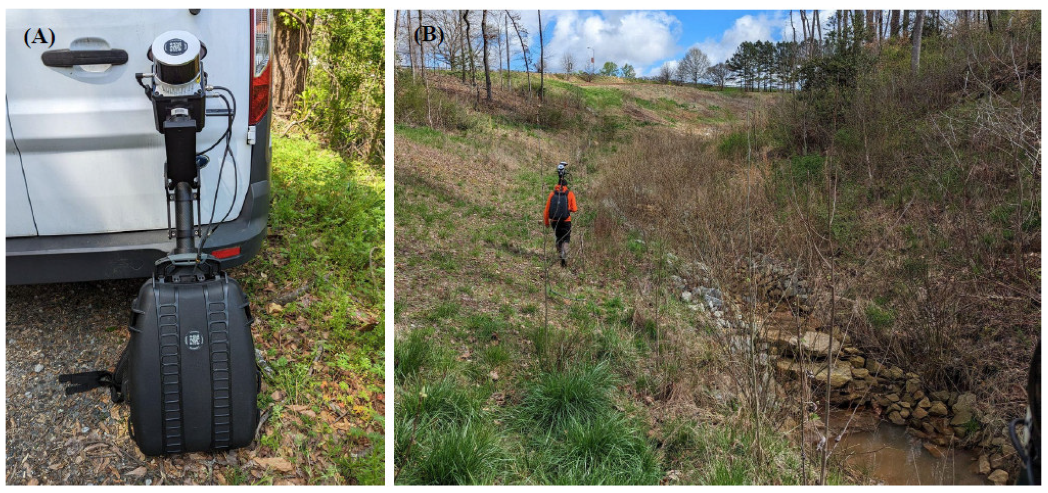
2.3. Terrestrial LiDAR and 3D River Channel Modeling

LiDAR data were collected at each station location using a backpack-mounted Surveyor 32-channel laser by LiDAR USA (Figure 4). This sensor is equipped with Snoopy GNSS IMU with a position accuracy of 0.01–0.005 m and can capture up to 1,280,000 points per second [60]. The sensor was connected to a GPS unit to ensure proper geolocation of the LiDAR datasets collected. Then, the data collector walked up and down the stream channel at the station locations with the backpack unit. The LiDAR point cloud data was post-processed to improve position accuracy.
The resulting LiDAR datasets were classified into ground or non-ground points using LAStools [61] using a step size of 1, a bulge value of 2, a spike of 1, a down spike of 1, an offset of 0.05, and ‘extra’ detail. These specifications help the program determine what points are ground and not ground and were determined to produce the most accurate point classification for the study area. The classified group points were converted into a DEM surface representing the stream channel ground using a cell size that was double the LiDAR point spacing for each file [62]. The DEMs were clipped only to include the upstream area of the water level sensor. The DEM surfaces were visualized in ArcScene 10.8.1 [63] using a custom base height to illustrate the elevation and stream channel morphology.
Water level planes were created to represent visualizations of different water level heights at each station location. These water level planes were created by making a raster the size of the station’s DEM and giving the raster a single elevation measurement. This raster could then be visualized along with the station’s 3D stream channel to represent what areas of the stream channel would be filled with water because of the chosen elevation for the water level.
The DEMs created from the LiDAR data were also evaluated for their overall mean slope to better understand the morphology of the stream channel sections.

2.4. Upstream Volume Calculations

The volume of water upstream of each sensor location was calculated to translate the 3D visualization models into data that can provide more information to hydrologists and stream managers. Water volume was calculated for each station location using ArcPro version 3.1, a popular geospatial analysis software [63] at a typical base-level flow scenario and a high water level scenario using the station’s DEM. These base level and high water level values were determined by examining the 2022 datasets to understand the largest change in water level for each site. A base level flow is the average water level for the station outside of storm events and illustrates the amount of flow typically present in the stream channel. The high water level scenarios were selected from each station’s change in water level data from 2022 and represented the average highest water level observed by the sensor at that station. Some station locations have water level sensors placed inside stormwater pipes with a fixed known diameter. When examining the maximum change in water level at each location, none of the changes seen in 2022 exceeded the pipe diameters, so the volume calculations represent the actual volume seen at each location. However, it is possible that in past years or future years, the water levels could rise above the pipe diameters, which would go beyond the range of the water level sensor. Water levels could rise higher than the sensor in the pipe, but the sensor would only be able to measure a maximum distance.
Changes in water volume for base flow and high water levels were also calculated for 2-foot cross-sectional areas around the water level sensor location. The DEMs for each station location were trimmed to only include one foot of width on either side of the sensor and extended horizontally across the entire stream width, forming a skinny cross-sectional area. Then, the volume in this 2-foot cross-section area was calculated for base flow and high water levels. By focusing on the 2 feet surrounding the sensor, the change in water level value derived from the machine learning analysis could be converted into the corresponding volume directly at the sensor area.

3. Results

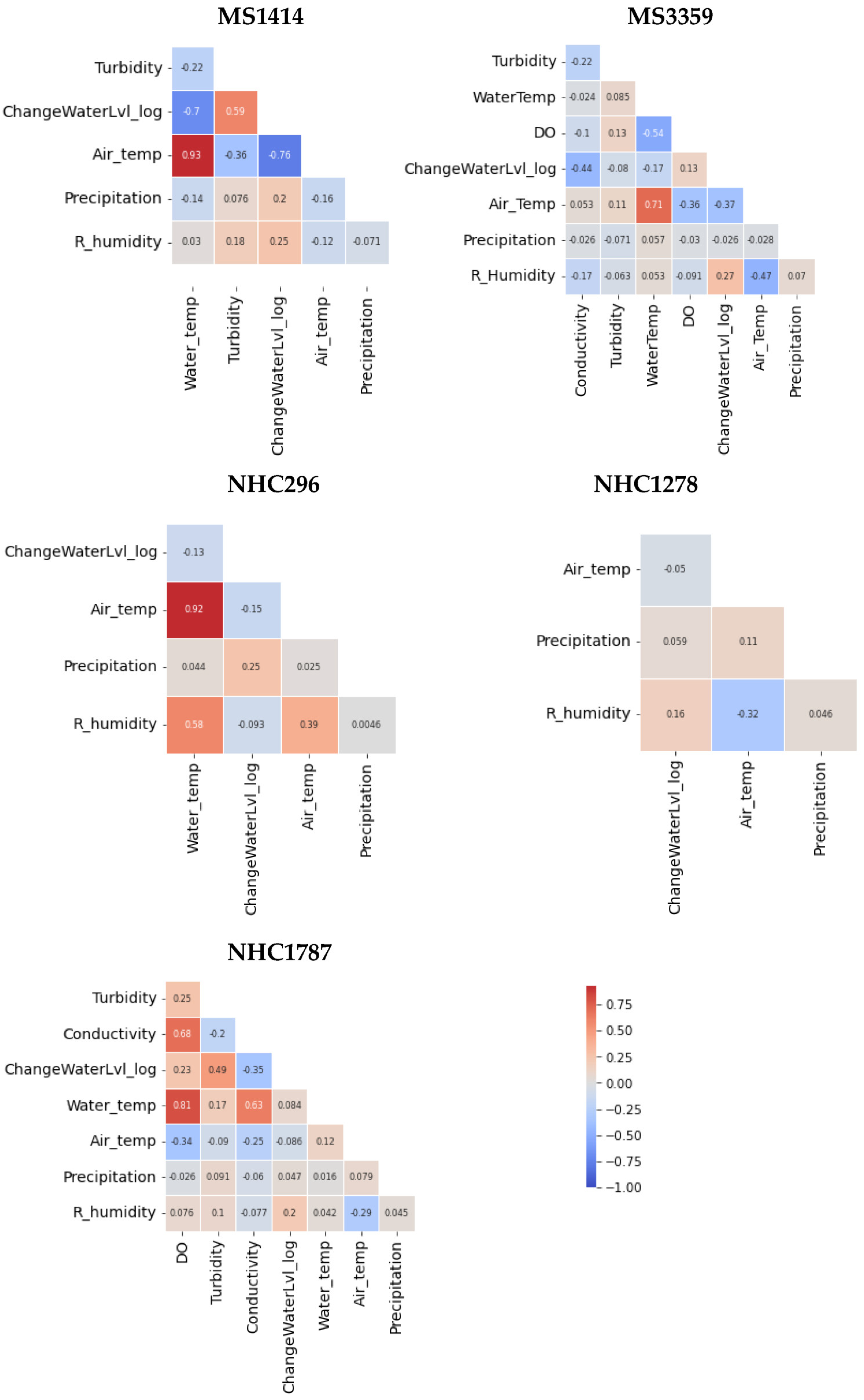
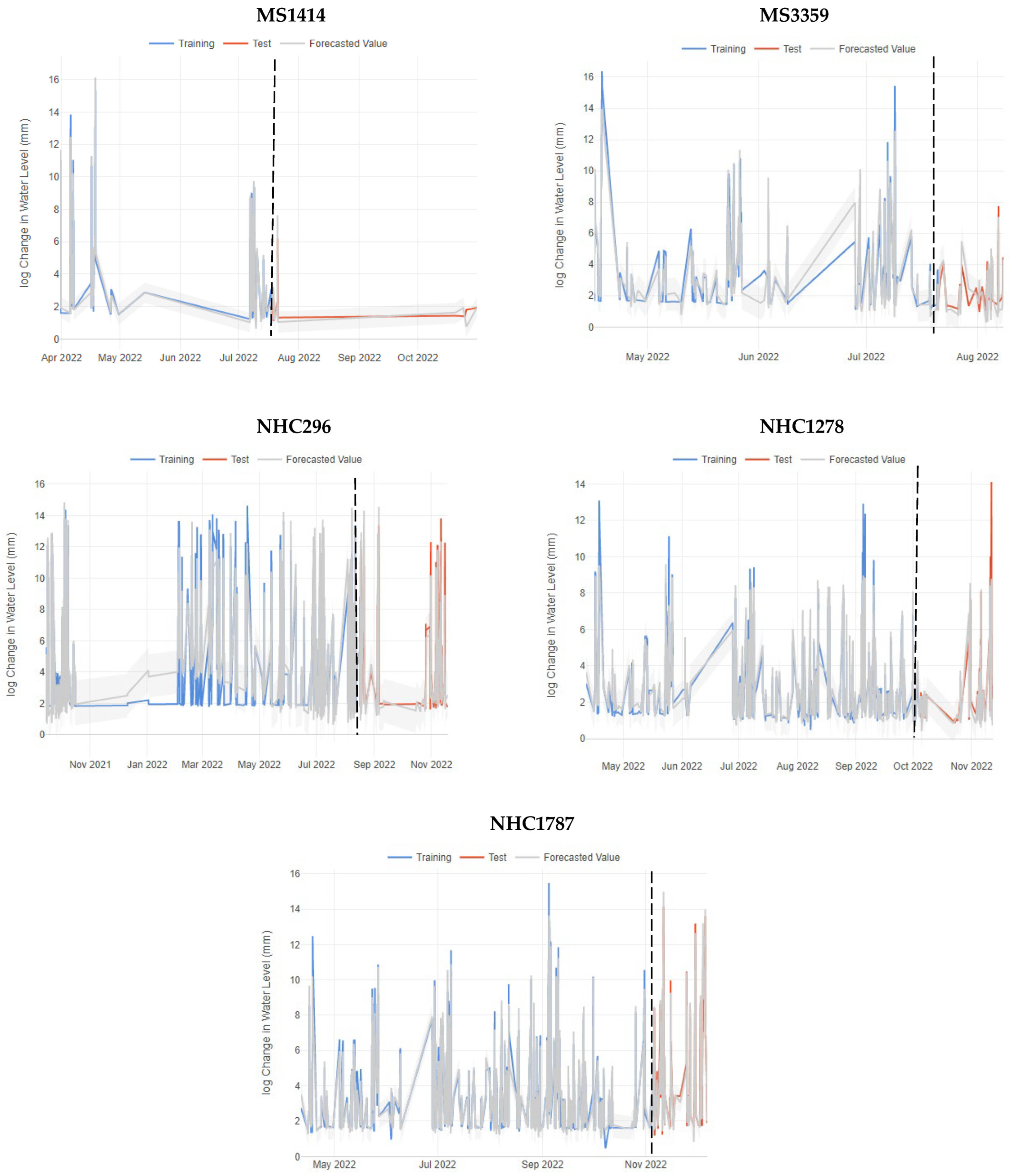
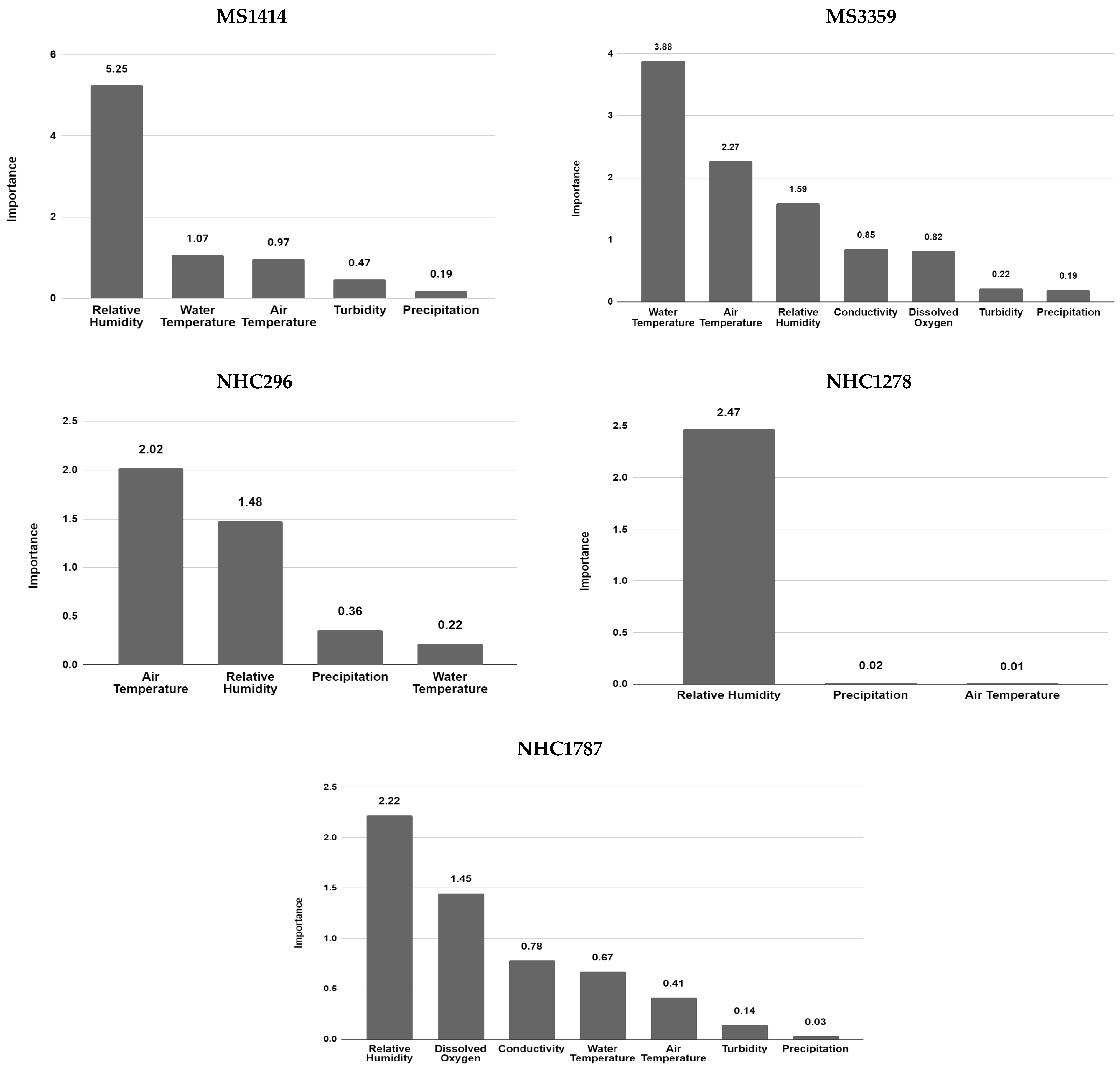
3.1. Machine Learning

Each station location in Hunnicutt measures a different combination of water quality and quantity variables due to the sensors placed at these locations. Some stations have sensors that capture many variables, and some stations only capture changes in water level. Examining the correlations of the datasets for each location tests to see if any of the variables have linear relationships (Figure 5). However, it is common for there to be a lack of strong linear relationships between hydrologic datasets because the interactions between variables are complex and not always directly related [64].
At station MS1414, the strongest positive data correlation was between air temperature and water temperature (0.93), followed by the correlation between the change in water level and turbidity (0.59). There was a moderate negative correlation between the change in water level and water temperature (−0.7) and between the change in water level and air temperature (−0.76). This is likely because air and water temperature may decrease during storm events, which causes water levels to increase. At station MS3359, the strongest positive correlation is also between the air and water temperature (0.71). A moderate negative correlation exists between dissolved oxygen and water temperature (−0.54), which is a natural phenomenon because colder water can hold more dissolved oxygen. The change in water level at this site has a moderate negative correlation with conductivity (−0.44). At station NHC296, air temperature and water temperature are strongly correlated (0.92), and water temperature is moderately correlated with relative humidity (0.58). The change in water level at this station only has weak correlations with the weather predictor variables and water temperature. Station NHC1286 only has weather station variables, which are weakly correlated with changes in water level.
Overall, this site has negligible correlations between any of the variables. At station NHC1876, conductivity correlates with dissolved oxygen (0.68) and water temperature (0.63). The change in water level moderately correlates with turbidity (0.49) and negatively with conductivity (−0.35).
The lack of strong correlations between change in water level and the other variables indicates that the relationships are nonlinear. This indicates that it is necessary to use a nonlinear regressor machine learning algorithm to predict changes in water level. Despite a lack of a clear relationship between dependent variables and changes in water level, a nonlinear regressor algorithm can still detect mathematical relationships in the data that are not described by physical mechanisms, illustrating the advantage of applying machine learning to complicated phenomena, such as hydrology problems [64,65].
Prophet is a nonlinear time series machine learning, and it successfully predicted future changes in water level at the hourly level for the selected station locations, evidenced by R2 scores greater than 0.9 at all stations (Table 2). Station MS1414 has the highest R2 score and lowest RMSE and MAE scores, meaning the time series algorithm had the most accurate change in water level predictions (Figure 6). The algorithm for station MS1414 used five variables to predict the change in water level. However, this site had the shortest time for data availability due to sensor outages at this location, meaning there was a smaller amount of testing data, which could contribute to an inflated accuracy.
Station MS3359 had seven input variables, which resulted in high R2 (0.944) and low RMSEs (0.535) and MAEs (0.433). The algorithm for station NHC296 had four input variables and the most data available over the longest period of time. This station had the highest RMSE and MAE values, meaning there was a greater difference between the predictions and true change in water level values, which could be because of frequent increases and decreases in water levels at this station compared to the other stations.
The algorithm at station NHC1278 had the lowest R2 scores, most likely due to only having three predictor variables coming from the weather station data and no data from the water quality at the water level station itself. There are fewer data inputs at this site because the sensor placed here is only calibrated to capture changes in water level and not the other water quality metrics seen at other sites. This could also be why the RMSE score is higher than most of the other stations (0.813).
The algorithm at site NHC1787 performed well with a high R2 score (0.964) and had seven predictor variables, like MS2259. The RMSE score was a little higher (0.729), and Figure 6 indicates that the model had trouble predicting some of the largest increases in water level.
There were slight differences between the five station locations due to the data available at each site, but overall, the Prophet algorithm was able to predict the changes in water level accurately. For all station locations, the variable with the lowest feature importance score was removed from the model, and the performance metrics were compared to those using all available variables. For all stations, removing the variable with the lowest feature importance decreased the R2 values slightly and increased the error metrics, meaning that despite low feature importance, the variable still contributed some information to enable the model to predict change in water level scores.
Examining the feature importance for each station provides information about what input variables had the greatest impact on the model’s change in water level predictions (Figure 7). At station MS1414, relative humidity had the greatest feature importance for the model, followed by air temperature. Air temperature had a high negative correlation with the change in water level, so this variable helped predict the future changes in water level at this station. This is likely because air temperatures tend to decrease during storm events, resulting in increased water levels. Interestingly, for four of the five station locations, precipitation had the lowest feature importance contributing to the model’s ability to predict changes in water level. However, when the precipitation variable was removed from the algorithms at each site, the model performance decreased, indicating that precipitation still plays a small role in helping the model predict future changes in water level.
At station MS2259, the water temperature had the greatest feature importance for predicting the change in water level despite the low correlation between the two variables. Water temperature also had the greatest feature importance at station NHC296, while air temperature had the lowest feature importance. Relative humidity had the greatest feature importance at station NHC1278. Dissolved oxygen and conductivity had the greatest feature importance for the model at station NHC1876. These values indicate that different water quality dynamics are at play at each station location throughout Hunnicutt Creek, so it is important to consider each location independently.

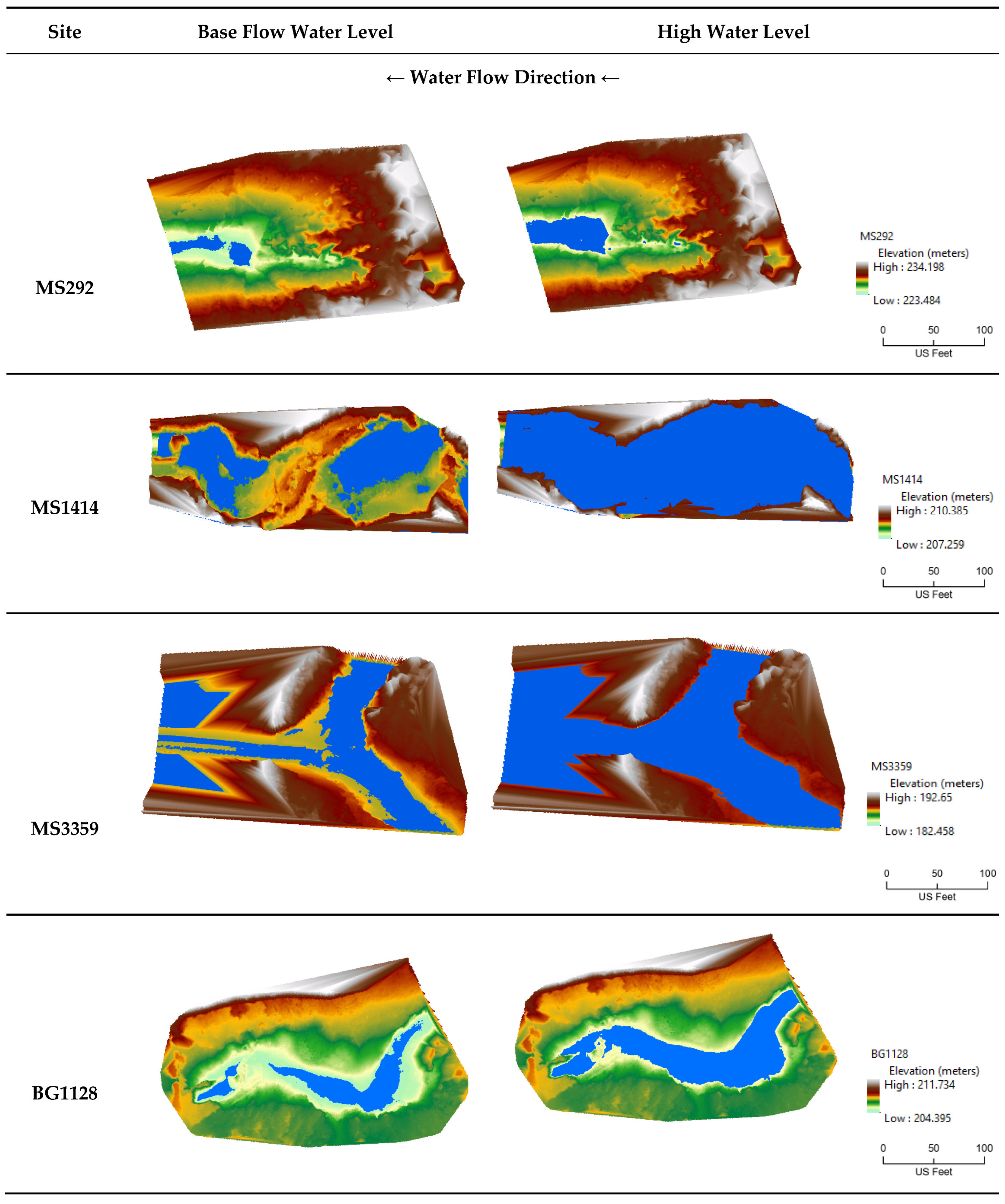
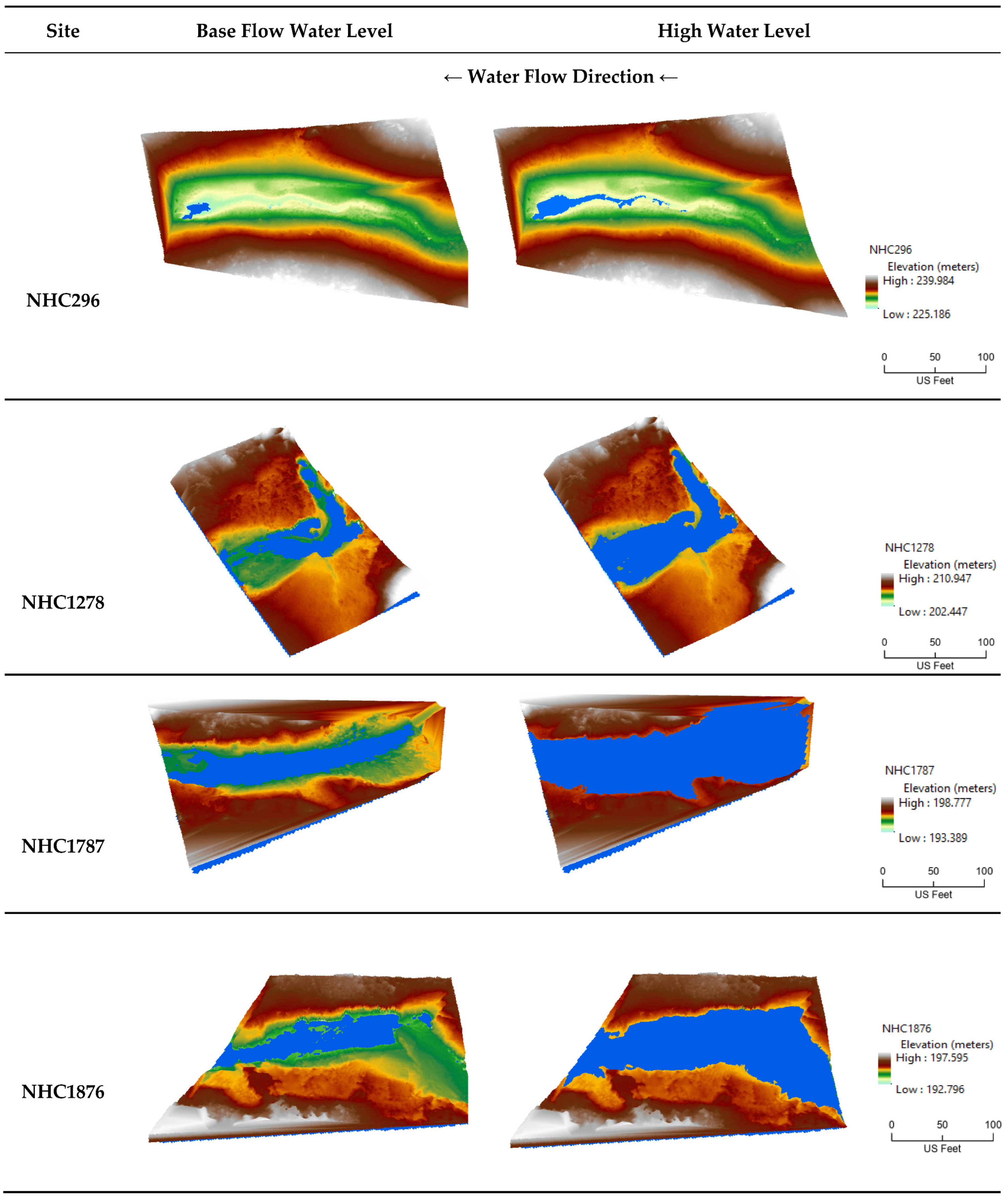
3.2. LiDAR 3D Models and Upstream Volume Calculations

The LiDAR sensor captured high-resolution data with point spacing ranging from 0.004 to 0.001, representing the average linear distance between points (Table 3). The point density for each LiDAR dataset is the number of points per square meter and is calculated by 1/(Point spacing)2, and this ranged from 10,000 to 62,500. This high level of detail from the LiDAR datasets then produced very precise DEMs with cell sizes ranging from 18 to 3 cm, providing highly detailed 3D surfaces representing the stream channels. These DEMs are much higher resolution than the previously generated DEMs for this area using aerial-flown aerial LiDAR, which had a resolution of 5 m per pixel.
Terrain analysis for each stream channel area was calculated to better understand the area’s morphology. The site’s mean slope indicates the steep elevation changes for that area. The mean slope percentages ranged from the lowest slope (26.5%) at station NHC1787 to the largest slope (36.5%) at site MS292.
The 3D DEMs showing the elevation changes and stream bank morphology provide useful visualizations to understand different water levels at a particular location (Figure 8 and Figure 9). Base flow and high-water levels that are typical for each site were used at each location to see which areas of the stream channel hold water during storm events and remain dry. The 3D terrain models can be rendered with different water levels to illustrate different conditions before, during, and after a storm. For instance, a change in water level prediction from the machine learning algorithm could be visualized in 3D for that site so stream managers could visually see the impact of the water level rise in the stream channel. The translation of the machine learning predictions to a 3D rendering helps non-machine learning experts make informed management decisions. To accompany these visualizations, water volume calculations were also determined at these sites to better understand how much water is present (Table 4).
Since station MS292 is upstream of an undisturbed, forested area, this station location typically does not experience water level rises greater than 0.63 m. A change in water level of this magnitude would result in an increase in upstream water volume of 39.59 m3. When just considering a two-foot cross-section at the water level sensor’s location, the water volume increases by 1.1145 m3, which gives more information about what is occurring at this particular location in the watershed.
The greatest increase in water level at station MS1414 was an 0.77 m increase, resulting in a 178.72 m3 increase in water volume. There was a 2.12 m3 increase in volume at the two-foot sensor location cross-section. The upstream area from the water level sensor placed in the wide metal pipe is a natural area, often with debris, sticks, and leaves that are visible when water levels are at base flow. During high water levels, the 3D stream channel model showed that these debris becomes submerged, and the whole stream channel filled with water, which then flows into the pipe.
Station MS3359 consists of a large concrete culvert, and the water level can increase by 1.05 m, resulting in an increase of 583.66 m3 of water volume in this concrete tunnel or 2.51 m3 at the two-foot cross-sectional area. This station has the largest increase in water volume seen in Hunnicutt Creek. During normal flow conditions, there is a constant flow of water through the concrete channel, and when the water level rises, the water expands further and higher in this channel, covering a larger surface area.
Station BG1128 is along a small section of Hunnicutt Creek, so the rise in water level at this site is typically lower at 0.4 m, which increases to 40.75 m3 in upstream water volume or 0.2 m3 in the two-foot cross-section area. Large rocks surround the mouth of this sensor (on the left), and during normal flow conditions, these are not submerged. However, when the water levels rise, the 3D model of the stream showed that the area becomes submerged.
At station NHC296, the water level can typically rise 1 m, causing an increase in upstream water volume of 38.64 m3 in the entire area or 2.21 m3 in the cross-sectional area around the sensor location. Despite this larger increase in water level, the 3D channel model illustrated that the channel is deep because there is no drastic change in the water in the channel. This area of Hunnicutt Creek was restored to have a more natural flow regime, illustrating that this area can accommodate a large quantity of water before the water rises to a high level in the downstream pipe outfall.
Station NHC1278 experienced water level rises of 0.43 m, resulting in an upstream volume increase of 74.41 m3 or 1.24 m3 in the two-foot cross-sectional area. The 3D model of this stream section showed that the sandy area in front of the two concrete pipes is typically dry, but during high water levels, the area is wide, and the water level rises to cover these sand banks before flowing into the pipes (to the left).
Station NHC1787 is a natural section of Hunnicutt Creek and has seen the water level rise 1.06 m, resulting in a water volume increase of 326.85 m3 in the upstream catchment and 4.3 m3 in the two-foot cross-section around the sensor. This area has a wide channel that allows water levels to spread out when more water volume is present.
Station NHC1876 is shortly downstream NHC1787 and is another natural area that typically experiences rises in water level of 0.9 m, which results in an increase of 99.72 m3 in water volume of the catchment area or 2.44 m3 in the two-foot cross-section area. This area also has a wide bank, so water is able to spread out in the channel.

4. Discussion

This methodology illustrates that the engineered, hardened channels of Hunnicutt Creek are more prone to flooding and high water levels than the more natural areas surrounded by vegetation. The station location with the most human impact at MS3359 with the wide hardened stream channel had the greatest observed increase in water levels and the change in volume due to storm events. The concrete culvert with hardened sides and bottom restricts the rise of Hunnicutt Creek, and, therefore, the water can rise rapidly when precipitation occurs. The larger increase in water volume at site MS3359 can also be attributed to its position in the Hunnicutt stream network because it is the most downstream site. More upstream water flow converges to this site location, causing larger increases in water level and, therefore, water volume.
In contrast, the location with the smallest change in upstream water volume during storm events is NHC296. Although the water level sensor at this location is placed in a concrete outfall pipe that captures the flow from upstream, this section of Hunnicutt was restored to have a wider, more natural floodplain. As seen in the 3D model for this site, the 0.9 m increase in water level causes the water in the stream channel to spread out and illustrates that the floodplain of the channel still has a large capacity to hold more water during a storm. The site with the second lowest change in upstream water volume during a storm event is MS292, located in a heavily wooded and undisturbed section of Hunnicutt Creek. Since this area of the stream is surrounded by tree cover and is a much less impervious area, there is not as dramatic of an increase in water level when it rains.
The Prophet machine learning algorithm was able to accurately predict future hourly changes in water level, as all sites had R2 values greater than 0.9. The performance of each algorithm at each site differed depending on the variables included at each station. This study shows that it is helpful to include water quality input data, such as water temperature, DO, and conductivity, in addition to weather variables like air temperature, relative humidity, and precipitation. Stations NHC296 and NHC1278 had fewer input variables and had lower R2 model performance as a result. Therefore, the algorithm at station NHC296 was not able to capture the extreme lows and highs as well as at the other locations, possibly due to the lower number of predictor variables that were not well-correlated with changes in water level. If additional water quality metrics are available, researchers should include them in the initial Prophet models to test if the additional data provides increased prediction power. Tyralis and Papacharalampous [19] similarly used the Prophet algorithm to forecast future streamflow levels at a monthly scale. In this study, they compared Prophet models that only used streamflow data to those also using temperature and precipitation data. The study concluded that streamflow predictions were similar regardless of the additional predictor data. It is important to examine different combinations of available variables when using the Prophet algorithms because additional variables may or may not improve performance. While the Prophet algorithm has been used to predict several time series-dependent variables, such as air temperature [66], precipitation [67,68], and groundwater levels [69], few studies have applied the algorithm to predict water level changes; our study is one of the first to do so.
The Prophet algorithm can accurately predict changes in water level with the input variables captured in this study because of the physical relationships between the parameters. The feature importance analysis illustrates that for the five sites examined, relative humidity, air temperature, and water temperature had the strongest relationship with changes in water level. Using these variables, the algorithm was able to predict future changes in water level. Relative humidity is the measure of how much water vapor is present in the air relative to the air temperature [70]. During rainfall events, relative humidity is high because of the large amounts of water vapor in the air. Therefore, relative humidity is an indirect measurement of precipitation and can be associated with storm events, which cause water levels to increase in Hunnicutt Creek. Relative humidity was more important to the Prophet algorithms to predict changes in water level over the precipitation data collected. This could be because of errors associated with the precipitation data collected in the study area that disrupted the relationship between precipitation and rises in water level, or it could be a result of a lag between precipitation and the resulting change in water level that was not captured in the hourly time data. Air and water temperature were also important predictor variables for the algorithms, likely because these values decrease during storm events [71]. Since these variables also serve as indirect measurements of storm events, they were important for Prophet in making predictions for water-level changes. It is also important to note that machine learning is adept at finding subtle relationships between variables that are not obvious to humans and can make predictions based on hidden data relationships.
Utilizing feature importance in machine learning analysis is also beneficial because it can inform what explanatory variables are included in the final algorithm. Since feature importance illustrates what explanatory variables contribute the most and the least to the final model prediction, researchers can remove the variable with the lowest feature importance score. By then comparing the overall model performance before and after removing the explanatory variable, researchers can decide if that variable can be excluded from the modeling or not. In this study, precipitation had the lowest feature importance score for three of the five sites (MS1414, MS3359, and NHC1787). Water temperature had the lowest feature importance at site NHC296, and both precipitation and air temperature had very low feature importance scores at site NHC1278. For each of these sites, the Prophet model performance was calculated both with and without these variables with the lowest feature importance scores. Model performance (R2) decreased for all sites when the variables were removed, and the errors in predictions increased (RMSE and MAE). Therefore, in this study, all variables were kept in the final Prophet algorithms. This decision was made because although the feature importance was low, the variables were still contributing some hidden information to the final change in water level predictions. Since the sensors in this study area already have a low number of explanatory variables (varying from three to seven), removing one was not beneficial for this study area. However, researchers applying feature importance analysis to their machine learning algorithms in other urban watersheds may find that removing the explanatory variables with low feature importance does not greatly impact the overall model accuracy and errors. Therefore, it might be beneficial to the researchers to remove that variable or several variables from the analysis, making the algorithm simpler and reducing the need for collecting additional information. Overall, using the feature importance analysis can help researchers determine the final datasets and input variables that are best for their study area; this is an important analysis step in practical forecasting.
This study was able to predict changes in water level at an hourly timescale, which can inform stream and risk managers about upcoming water level rises and resulting flooding in Hunnicutt Creek. As the water level, water quality, and weather station sensors deployed in Hunnicutt Creek continue to gather data over time, and as improvements are continued to be made to decrease missing data points, these developed algorithms should continue to improve with a longer time frame of available data. In addition, with a greater amount of temporal input data, future research should continue to refine these algorithms to increase the temporal resolution and predict changes in water level at smaller time scales, such as thirty- or fifteen-minute increments. This improvement in temporal scale in the future could continue to help Hunnicutt managers because urban streams are flashy, with rapid water level rises and falls that may not be fully captured at the current hourly time scale.
The change in water level predictions will assist the Hunnicutt managers in forecasting upcoming periods of changes in water level. However, this machine learning information alone does not provide a complete flood analysis for Hunnicutt Creek. The addition of terrestrial LiDAR scanning, 3D modeling, and stream volume calculations provides a richer analysis that can fully explore the flood potential of the urban stream. For instance, the predictions from the machine learning models can be converted into water level rasters that can now be visualized in the 3D stream channel models to visualize what that change in water level would look like. This translation into the 3D model will help risk managers see what areas will flood and what areas will hold water during a storm event. Managers can also examine the DSMs that illustrate the vegetation present at each site to see what vegetation will be submerged and impacted during a rise in water level. Studies have found that understanding the microtopography of stream channels is critical to flood models and improving stream management strategies for climate change planning [72,73].
Terrestrial LiDAR scanning produced high-resolution point clouds and resulting DEMs produced highly accurate flood inundation models. Other studies have similarly found that using terrestrial LiDAR produces the most accurate DEMs for analyzing flooding and is a better methodology than relying only on airborne LiDAR [73,74,75]. In watersheds with heavily vegetated riparian buffers and low-lying vegetation, using terrestrial LiDAR is preferred to use unmanned aerial vehicle (UAV)-mounted LiDAR because the UAV would not be able to fly close to the stream and, therefore, produce lower resolution data.
Terrestrial LiDAR scanning produced highly detailed stream morphology 3D models. However, it is important to note that LiDAR does not penetrate water, so the scans and resulting DEMs do not display the true stream bottoms. In Hunnicutt Creek, the base flow conditions are very low, so this impact was negligible in the model creations, but it should be considered for urban streams that have deeper waters at normal conditions. Researchers could compensate for this by capturing the terrestrial LiDAR after periods of no recent precipitation so that base flow is lowest. Despite the models including some level of stream base flow, the methodology still allows the modeling of large increases in water level.

Methodology Applications

This study’s proposed methodology to examine urban stream flood potential can be used by a variety of scientists and professionals to combat the negative impacts of urban flooding. Identifying what areas of the watershed have poor drainage and experience large changes in water level provides stormwater managers with knowledge about areas that may need more infrastructure such as drains, culverts, or other best management practices to combat flooding areas. For instance, studies have found that ecological management practices (EMPs) such as bio-retention areas, infiltration trenches, and green roofs can effectively reduce the rapid increase in water levels [76]. Similarly, knowing what areas tend to have rapid changes in rising water levels can help stream managers know what areas would benefit from restoration efforts, such as graduating banks to slow stormwater runoff into the stream, therefore slowing the change in water levels and decreasing flood likelihood. This study’s machine learning prediction capabilities allow risk management officers to forecast future flood scenarios and give them time to prepare accordingly. Similar studies have explored other machine learning algorithms, such as random forest, to predict future flood events for risk management [77,78].
Ecosystem scientists can use the 3D models and water level models to understand what areas are most at risk for the negative impacts of flooding, including loss of vegetation, erosion, stream bank collapse, and sedimentation. For instance, in this study, the upstream area to MS292 has the greatest mean slope due to tall, steep stream banks. While the taller banks mean that the water level can rise higher without causing flooding, this slope could cause stream bank failures or collapses due to overland flow into the stream. In contrast, the NHC1787 upstream area had the lowest mean slope and has a wider, shallower stream channel. The 3D model illustrates that this area experiences a drastic change in water level and a large increase in water volume that spreads out in the channel. This wider area of rising water level could cause greater impacts on surrounding vegetation.
After establishing the current stream morphology with LiDAR scanning and 3D models, researchers could scan the watersheds again after a fixed time and compare the DEMs and 3D models to understand erosion and sediment deposition in the watershed. As illustrated by several recent studies [79,80], this can provide more information on where stream banks are incising and where the stream channels are being filled in with sediment, which has been performed in several recent studies.

5. Conclusions

This study establishes a methodology to analyze urban stream flooding by combining machine learning using the Prophet algorithm with terrestrial LiDAR scanning to create 3D flooding models and stream water volume calculations. The Prophet algorithm can accurately forecast future changes in water level from weather input variables such as precipitation, air temperature, and relative humidity. Additional water quality variables such as DO, conductivity, and water temperature provide more data to the algorithms, improving the predictions. The terrestrial LiDAR captured by the backpack-mounted laser resulted in high-resolution DEMs from 1.8 to 3 cm. Thus, very high-resolution 3D models were created to visualize changes in water level at each location along Hunnicutt Creek. These 3D models can be used to visualize changes in water level predictions from the machine learning output, providing more information to stream managers about potential flooding. Therefore, stream and stormwater managers can use this methodology to analyze water level changes in Hunnicutt Creek better to understand the flood-prone areas on Clemson’s campus. In addition, the data can be used by a variety of other experts to analyze what areas of the watershed are at the highest risk for erosion, sedimentation, stream bank loss, and structural damage due to flooding. With climate change, urban streams will continue to face frequent, heavy storm events, so methodologies such as these proposed herein are necessary to learn about and plan for future flood scenarios.

Author Contributions

Conceptualization, M.M.B. and C.J.P.; methodology, M.M.B.; C.J.P., M.Z.N. and F.F.; software, M.M.B., C.J.P. and M.Z.N.; validation, M.M.B.; formal analysis, M.M.B.; data curation, M.M.B.; writing—original draft preparation, M.M.B.; writing—review and editing, M.M.B., C.J.P., M.Z.N., F.F. and E.A.M.; visualization, M.M.B.; supervision, C.J.P. All authors have read and agreed to the published version of the manuscript.

Funding

This research received no external funding.

Data Availability Statement

The data presented in this study are available upon request from the corresponding author.

Acknowledgments

Thank you to the Intelligent Rivers® Hunnicutt Creek project for access to their Hunnicutt Creek sensor network data used in this study. We would also like to thank the Clemson Center for Geospatial Technologies for their assistance in collecting the LiDAR data.

Conflicts of Interest

The authors declare no conflict of interest.

References

  1. Kim, S.; Tachikiawa, Y.; Takara, K. Recent flood disasters and progress of disaster management system in Korea. Annu. Disaster Prev. Res. Inst. 2007, 50, 15–31. [Google Scholar]
  2. Walsh, C.J.; Roy, A.H.; Feminella, J.W.; Cottingham, P.D.; Groffman, P.M.; Morgan, R.P. The urban stream syndrome: Current knowledge and the search for a cure. J. N. Am. Benthol. Soc. 2005, 24, 706–723. [Google Scholar] [CrossRef]
  3. Wilson, C.; Weng, Q. Assessing surface water quality and its relation with urban land cover changes in the Lake Calumet Area, Greater Chicago. Envion. Manag. 2010, 45, 1096–1111. [Google Scholar] [CrossRef]
  4. Wilby, R.; Perry, G.L.W. Climate change, biodiversity and the urban environment: A critical review based on London, UK. Prog. Phys. Geogr. 2006, 30, 73–98. [Google Scholar] [CrossRef]
  5. Sun, N.; Yearsley, J.; Baptiste, M.; Cao, Q.; Lettenmaier, D.; Nijssen, B. A spatially distributed model for assessment of the effects of changing land use and climate change on urban stream quality. Hydrol. Process. 2016, 30, 4779–4798. [Google Scholar] [CrossRef]
  6. Bell, C.D.; McMillan, S.K.; Clinton, S.M.; Jefferson, A.J. Hydrologic response to stormwater control measures in urban watersheds. J. Hydrol. 2016, 541, 1488–1500. [Google Scholar] [CrossRef] [Green Version]
  7. Konrad, C.P.; Booth, D.B. Hydrological changes in urban streams and their ecological significance. Am. Fish. Soc. Symp. 2005, 47, 157–177. [Google Scholar]
  8. Paul, M.J.; Meyer, J.L. Streams in the urban landscape. Annu. Rev. Ecol. Syst. 2001, 32, 333–365. [Google Scholar] [CrossRef]
  9. Awadallah, M.O.; Juarez, A.; Alfredsen, K. Comparison between topographic and bathymetric LiDAR terrain models in flood inundation estimations. Remote Sens. 2022, 14, 227. [Google Scholar] [CrossRef]
  10. Ourloglou, O.; Stefanidis, K.; Dimitriou, E. Assessing nature-based and classical engineering solutions for flood-risk reduction in urban streams. J. Ecol. Eng. 2020, 21, 46–56. [Google Scholar] [CrossRef]
  11. Kolakovic, S.; Kolakovic, S.; Fabian, J.; Jeftenic, G.; Trajkovic, S. River floodplain 1D/2D hydraulic modeling combined with recent LiDAR DTM technology. Tech. Gaz. 2021, 28, 880–890. [Google Scholar] [CrossRef]
  12. Bruno, L.S.; Mattos, T.S.; Oliveira, T.S.; Almagro, A.; Rodrigues, D.B.B.R. Hydrological and hydraulic modeling applied to flash flood event in a small urban stream. Hydrology 2022, 9, 223. [Google Scholar] [CrossRef]
  13. Brunner, G.W. HEC-RAS 5.0 Hydraulic Reference Manual; US Army Corps of Engineers: Washington, DC, USA, 2016.
  14. Baek, S.S.; Pyo, J.; Chun, J.A. Prediction of water level and water quality using a CNN-LSTM combined deep learning approach. Water 2020, 12, 3399. [Google Scholar] [CrossRef]
  15. Phan, T.; Nguyen, X.H. Combining statistical machine learning models with ARIMA for water level forecasting: The case of the Red River. Adv. Water Resour. 2020, 142, 103656. [Google Scholar] [CrossRef]
  16. Ghorpade, P.; Gadge, A.; Lende, A.; Chordiya, H.; Gosavi, G.; Mishra, A.; Hooli, B.; Ingle, Y.S.; Shaikh, N. Flood forecasting using machine learning: A review. In Proceedings of the 8th International Conference on Smart Computing and Communication (ICSCC), Kochi, India, 1–3 July 2021. [Google Scholar] [CrossRef]
  17. Mosavi, A.; Ozturk, P.; Chau, K. Flood prediction using machine learning models: Literature review. Water 2018, 10, 1536. [Google Scholar] [CrossRef] [Green Version]
  18. Sahoo, B.B.; Jha, R.; Singh, A.; Kumar, D. Long short-term memory (LSTM) recurrent neural network for low-flow hydrological time series forecasting. Acta Geophys. 2019, 67, 1471–1481. [Google Scholar] [CrossRef]
  19. Tyralis, H.; Papacharalampous, A. Large-scale assessment of Prophet for multi-step ahead forecasting of monthly streamflow. Adv. Geosci. 2018, 45, 147–153. [Google Scholar] [CrossRef] [Green Version]
  20. Munoz, P.; Orellana-Alvevar, J.; Bendix, J.; Feyen, J.; Celleri, R. Flood early warning systems using machine learning techniques: The case of the Tomebamba Catchment at the southern Andes of Ecuador. Hydrology 2021, 8, 183. [Google Scholar] [CrossRef]
  21. Nevo, S.; Morin, E.; Rosenthal, A.G.; Metzger, A.; Barshai, C.; Weitzner, D.; Voloshin, D.; Kratzert, F.; Elidan, G.; Dror, G.; et al. Flood forecasting with machine learning models in an operational framework. Hydrol. Earth Syst. Sci. 2022, 26, 4013–4032. [Google Scholar] [CrossRef]
  22. Rasheed, Z.; Aravamudan, A.; Sefidmazgi, A.G.; Anagnostopoulos, G.C.; Nikolopoulos, E.I. Advancing flood warning procedures in ungauged basins with machine learning. J. Hydrol. 2022, 609, 127736. [Google Scholar] [CrossRef]
  23. Liu, Y.; Wang, H.; Feng, W.; Huang, H. Short term real-time rolling forecast of urban river water levels based on LSTM: A case study in Fuzhou City, China. Int. J. Eng. Res. Public Health 2021, 18, 9287. [Google Scholar] [CrossRef] [PubMed]
  24. Koyama, M.; Sakai, M.; Yamada, T. Study on water-level-forecast method based on a time series analysis of urban river basins—A case study of Shibuya River Basin in Tokyo. Water 2022, 15, 161. [Google Scholar] [CrossRef]
  25. Moon, H.; Yoon, S.; Moon, Y. Urban flood forecasting using a hybrid modeling approach based on a deep learning technique. Hydroinformatics 2023, 25, 593–610. [Google Scholar] [CrossRef]
  26. Wanginger, U. Introduction to LiDAR. In LiDAR; Weitkamp, C., Ed.; Springer Series in Optical Sciences; Springer: New York, NY, USA, 2005; Volume 102, pp. 1–18. ISBN 9780387400754. [Google Scholar]
  27. Liu, X. Airborne LiDAR for DEM generation: Some critical issues. Prog. Phys. Geogr. 2008, 32, 31–49. [Google Scholar] [CrossRef]
  28. Young, A.P.; Olsen, M.J.; Driscoll, N.; Flick, R.E.; Gutierrez, R.; Guza, R.T.; Johnstone, E.; Kuester, F. Comparison of airborne and terrestrial Lidar estimates of seacliff erosion in Southern California. Photogramm. Eng. Remote Sens. 2010, 76, 421–427. [Google Scholar] [CrossRef] [Green Version]
  29. Williams, K.; Olsen, M.J.; Roe, G.V.; Glennie, C. Synthesis of transportation applications of mobile LiDAR. Remote Sens. 2013, 5, 4652–4692. [Google Scholar] [CrossRef] [Green Version]
  30. Wang, G.; Joyce, J.; Phillips, D.; Shrestha, R.; Carter, W. Delineating and defining the boundaries of an active landslide in the rainforest of Puerto Rico using a combination of airborne and terrestrial LiDAR data. Landslides 2013, 10, 503–513. [Google Scholar] [CrossRef]
  31. Dong, W. 3D modeling of UC Berkeley’s Strawberry Creek using terrestrial LiDAR. In Proceedings of the Environmental Sciences Senior Thesis Symposium, Berkeley, CA, USA, 14 April 2018; pp. 1–34. [Google Scholar]
  32. Myers, D.T.; Rediske, R.R.; McNair, J.N. Measuring streambank erosion: A comparison of erosion pins, total station, and terrestrial laser scanner. Water 2019, 11, 1846. [Google Scholar] [CrossRef] [Green Version]
  33. Costabile, P.; Costanzo, C.; Lorenzo, G.; Santis, R.S.; Penna, N.; Macchione, F. Terrestrial and airborne laser scanning and 2-D modeling for 3-D flood hazard maps in urban areas: New opportunities and perspectives. Environ. Modell. Sofw. 2021, 135, 104889. [Google Scholar] [CrossRef]
  34. Ramacgabdran, R.; Fernandez, Y.B.; Truckell, I.; Constantiono, C.; Casselden, R.; Leinster, P.; Casado, M.R. Strategies for the characterization of microtopographic features that influence surface water flooding. Remote Sens. 2023, 15, 1912. [Google Scholar] [CrossRef]
  35. Bolick, M.M.; Post, C.J.; Naser, M.Z.; Mikhailova, E.A. Comparison of machine learning algorithms to predict dissolved oxygen in an urban stream. Environ. Sci. Pollut. Res. 2023, 30, 78075–78096. [Google Scholar] [CrossRef] [PubMed]
  36. U.S. Climate Data. Available online: https://www.usclimatedata.com/climate/pickens/south-carolina/united-states/ussc0270 (accessed on 3 April 2023).
  37. Esswein, S.; Hallstrom, J.; Post, C.J.; White, D.; Eidson, G. Augmenting hydrologic information systems with streaming water resource data. In Proceedings of the South Carolina Water Resources Conference, Columbia, SC, USA, 13–14 October 2010. [Google Scholar]
  38. Taylor, S.J.; Letham, B. Forecasting at scale. Am. Stat. 2017, 72, 37–45. [Google Scholar] [CrossRef]
  39. Harvey, A.; Peters, S. Estimation procedures for structural time series models. J. Forecast. 1990, 9, 89–108. [Google Scholar] [CrossRef]
  40. Chowdari, K.K.; Barma, S.D.; Bhat, N.; Girisha, R.; Gouda, K.C. Evaluation of ARIMA, Facebook Prophet, and a boosting algorithm framework for monthly precipitation prediction of a semi-arid district of north Karnataka, India. In Proceedings of the Fourth International Conference on Emerging Research in Electronics, Computer Science, and Technology (ICERECT), Mandya, India, 26–27 December 2022; pp. 1–5. [Google Scholar] [CrossRef]
  41. Xiao, Q.; Zhou, L.; Xiang, X.; Liu, L.; Liu, X.; Li, X.; Ao, T. Integration of hydrological model and time series model for improving the runoff simulation: A case study on BTOP modeling in Zhou River Basin, China. Appl. Sci. 2022, 12, 6883. [Google Scholar] [CrossRef]
  42. Khatibi, R.; Ghorbani, M.A.; Naghipour, L.; Jothiprakash, V.; Fathima, T.A.; Fazelifard, M.H. Inter-comparison of time series models of lake levels predicted several modeling strategies. J. Hydrol. 2014, 511, 530–545. [Google Scholar] [CrossRef]
  43. Yaseen, Z.M.; Naghshara, S.; Salih, S.Q.; Kim, S.; Malik, A.; Ghorbani, M.A. Lake water modeling using newly developed hybrid data intelligence model. Theor. Appl. Climatol. 2020, 141, 1285–1300. [Google Scholar] [CrossRef]
  44. Du, N.; Liang, X. Short-term water level prediction of Hongze Lake by Prophet-LSTM combined model based on LAE. In Proceedings of the 7th International Conference on Hydraulic and Civil Engineering & Smart Water Conservancy and Intelligent Disaster Reduction Forum, Nanjing, China, 6–8 November 2021. [Google Scholar]
  45. Tornevi, A.; Bergstedt, O.; Forsber, B. Precipitation effects on microbial pollution in a river: Lag structures and seasonal effect modification. PLoS ONE 2014, 9, e98546. [Google Scholar] [CrossRef]
  46. Van Vliet, M.T.H.; Ludwig, F.; Zwolsman, J.J.G.; Weedon, G.P.; Kabat, P. Global river temperatures and sensitivity to atmospheric warming and changes in river flow. Water Resour. Res. 2011, 47, W02544. [Google Scholar] [CrossRef]
  47. Oo, H.T.; Zin, W.W.; Kyi, C.C.T. Analysis of streamflow response to changing climate conditions using SWAT model. Civil. Eng. J. 2020, 6, 194–209. [Google Scholar] [CrossRef] [Green Version]
  48. Morrill, J.C.; Bales, R.C.; Conklin, M.H. Estimating stream temperature from air temperature: Implications for future water quality. J. Environ. Eng. 2005, 131, 139–146. [Google Scholar] [CrossRef] [Green Version]
  49. Yang, D.; Peterson, A. River water temperature in relation to local air temperature in the Mackensize and Yukon Basins. Arctic 2017, 70, 47–58. [Google Scholar] [CrossRef]
  50. Campolo, M.; Andreussi, P.; Soldati, A. River flood forecasting with a neural network model. Water Resour. Res. 1999, 35, 1191–1197. [Google Scholar] [CrossRef]
  51. Fleischmann, A.; Fan, F.; Collischonn, B.; Collischonn, W.; Pontes, P.; Ruhoff, A. Precipitation as a proxy for climate variables: Application for hydrological modelling. Hydrol. Sci. Res. 2019, 64, 361–379. [Google Scholar] [CrossRef]
  52. Harvey, R.; Lye, L.; Khan, A.; Paterson, R. The influence of air temperature on water temperature and the concentration of dissolved oxygen in Newfoundland Rivers. Can. Water Resour. J. 2013, 36, 171–192. [Google Scholar] [CrossRef]
  53. Rajwa-Kuligiewicz, A.; Bialik, R.J.; Rowinski, P.M. Dissolved oxygen and water temperature dynamics in lowland rivers over various timescales. J. Hydrol. Hydromech. 2015, 63, 353–363. [Google Scholar] [CrossRef] [Green Version]
  54. Irvine, K.N.; Richey, J.E.; Holtgrieve, G.W.; Sarkkula, J.; Sampson, M. Spatial and temporal variability of turbidity, dissolved oxygen, conductivity, temperature, and fluorescence in the lower Mekong River- Tonle Sap system identified using continuous monitoring. Int. J. River Basin Manag. 2011, 9, 151–168. [Google Scholar] [CrossRef]
  55. Ouali, D.; Chebana, F.; Ouarda, T.B.M.J. Fully nonlinear statistical and machine-learning approaches for hydrological frequency estimation at ungauged sites. J. Adv. Model. Earth Syst. 2017, 9, 1292–1306. [Google Scholar] [CrossRef]
  56. Wang, W.; Chau, K.; Cheng, C.; Qiu, L. A comparison of performance of several intelligence methods for forecasting monthly discharge time series. J. Hydrol. 2009, 374, 294–306. [Google Scholar] [CrossRef] [Green Version]
  57. Reich, N.G.; Lessler, J.; Sakrejda, K.; Lauer, S.A.; Iamsirithanworn, S.; Cummings, D.A.T. Case study in evaluating time series prediction models using the relative means absolute error. Am. Stat. 2016, 70, 285–292. [Google Scholar] [CrossRef] [Green Version]
  58. Chicco, D.; Warrens, M.J.; Jurman, G. The coefficient of determination R-squared is more informative than SMAPE, MAE, MAPE, MSE, and RMSE in regression analysis evaluation. PeerJ Comput. Sci. 2021, 7, e623. [Google Scholar] [CrossRef]
  59. Molnar, C. Interpretable Machine Learning: A Guide for Making Black Box Models Explainable; Learnpub: Victoria, BC, Canada, 2019. [Google Scholar]
  60. LiDAR USA. Surveyor 32. Available online: https://www.lidarusa.com/surveyor-32-uav-and-mms.html (accessed on 27 April 2023).
  61. Isenburg, M. LAStools, Efficient LiDAR Processing Software. Version 1.4, Academic. Available online: https://rapidlasso.com/LAStools (accessed on 27 April 2023).
  62. Chow, T.E.; Hodgson, M.E. Effects of lidar post-spacing and DEM resolution to mean slope estimation. Int. J. Geogr. Inf. Sci. 2009, 23, 1277–1295. [Google Scholar] [CrossRef]
  63. ESRI. ArcScene, version 10.8.1; ESRI: Redlands, CA, USA, 2023.
  64. Sun, X.Y.; Newham, L.T.H.; Croke, B.F.W.; Norton, J.P. Three complementary methods for sensitivity analysis of a water quality model. Environ. Modell. Softw. 2012, 37, 19–29. [Google Scholar] [CrossRef]
  65. Abrahart, R.J.; See, L.M. Neural network modeling of non-linear hydrological relationships. Hydrol. Earth Syst. Sci. 2007, 11, 1563–1579. [Google Scholar] [CrossRef] [Green Version]
  66. Asha, J.; Rishidas, S.; Santhosh Kumar, S.; Reena, P. Analysis of temperature prediction using random forest and Facebook Prophet algorithms. In Proceedings of the International Conference on Innovative Data Communication Technologies and Application (ICIDCA), Coimbatore, India, 17–18 October 2019; pp. 432–439. [Google Scholar]
  67. Okonkwo, S.; Ukoha, P.; Adedoyin, E.; Adewoye, R. Time series analysis of precipitation in Lake Chad using the Prophet Forecasting procedure. In Proceedings of the 4th International Conference of Professional Statisticians Society of Nigeria (PSSN), Ilorin, Nigeria, 24–27 August 2020. [Google Scholar]
  68. Sulasikin, A.; Nugraha, Y.; Kanggrawan, J.I.; Suherman, A.L. Monthly rainfall prediction using the Facebook Prophet model for flood mitigation in Central Jakarta. In Proceedings of the International Conference on ICT for Smart Society (ICISS), Bandung, Indonesia, 2–4 August 2021; pp. 1–5. [Google Scholar] [CrossRef]
  69. Aguilera, H.; Guardiola-Albert, C.; Naranjo-Fernandez, N.; Kohfahl, C. Towards flexible groundwater-level prediction for adaptive water management: Using Facebook’s Prophet forecasting approach. Hydrol. Sci. J. 2019, 64, 1504–1518. [Google Scholar] [CrossRef]
  70. Elovitz, K.M. Understanding what humidity does and why. ASHRAE J. 1999, 41, 84. [Google Scholar]
  71. Bao, J.; Sherwood, S.C.; Alexander, L.V.; Evans, J.P. Future increases in extreme precipitation exceed observed scaling rates. Nat. Clim. Change 2017, 7, 128–132. [Google Scholar] [CrossRef]
  72. Fatdillah, E.; Rehan, B.M.; Rameshwaran, P.; Bell, V.A.; Zulkafli, Z.; Yusuf, B.; Sayers, P. Spatial estimates of flood damage and risk are influenced by the underpinning DEM resolution: A case study in Kuala Lumpur, Malaysia. Water 2022, 14, 2208. [Google Scholar] [CrossRef]
  73. Sampson, C.C.; Fewtrell, T.J.; Duncan, A.; Shaad, K.; Horritt, M.S.; Bates, P.D. Use of terrestrial laser scanning data to drive decimetric resolution urban inundation models. Adv. Water Resour. 2012, 41, 1–17. [Google Scholar] [CrossRef]
  74. Turner, A.B.; Colby, J.D.; Csontos, R.M.; Batten, M. Flood modeling using a synthesis of multi-platform LiDAR data. Water 2013, 5, 1533–1560. [Google Scholar] [CrossRef] [Green Version]
  75. Ozdemir, H.; Sampson, C.C.; De Almeida, G.A.M.; Bates, P.D. Evaluating scale and roughness effects in urban flood modeling using terrestrial LiDAR data. Hydrol. Earth Syst. Sci. 2013, 17, 4015–4030. [Google Scholar] [CrossRef] [Green Version]
  76. Singh, A.; Sarma, A.K.; Hack, J. Cost-effective optimization of nature based solutions for reducing urban floods considering limited space availability. Environ. Proc. 2020, 7, 297–319. [Google Scholar] [CrossRef]
  77. Maspo, N.; Harun, A.N.B.; Goto, M.; Cheros, F.; Haron, N.A.; Nawi, M.N.M. Evaluation of machine learning approach in flood prediction scenarios and its input parameters: A systematic review. In Proceedings of the 7th AUN/SEED-Net Regional Conference on National Disaster, Kuala Lumpar, Malaysia, 25–26 November 2019; Volume 479. [Google Scholar] [CrossRef]
  78. Motta, M.; Neto, M.C.; Sarmento, P. A mixed approach for urban flood prediction using machine learning and GIS. Int. J. Disaster Risk Res. 2021, 56, 102154. [Google Scholar] [CrossRef]
  79. Brecheisen, Z.S.; Richter, D. Gully-erosion estimation and terrain reconstruction using analyses of microtropographic roughness and LiDAR. Catena 2021, 202, 105264. [Google Scholar] [CrossRef]
  80. Wolter, C.F.; Schilling, K.E.; Palmer, J.A. Quantifying the extent of eroding streambanks in Iowa. J. Am. Water Resour. Assoc. 2021, 57, 391–405. [Google Scholar] [CrossRef]
Figure 1. Hunnicutt Creek watershed and water level sensor and weather station locations. Water level sensors are named according to the branch of Hunnicutt Creek they are placed on and the distance the sensor is from the headwaters (MS = Main Stem; BG = Botanical Gardens; NHC = North Hunnicutt Creek). Weather stations are numbered 1–3.
Water 15 02581 g001
Figure 2. Examples of water level station locations throughout Hunnicutt Creek.
Water 15 02581 g002
Figure 3. Examples of Hunnicutt flooding during storm events: (A) aink hole formation along a road due to flooding, (B) high water level flowing into a stormwater pipe at site BG1128, (C) high water and flooding in Hunnicutt Creek with heavy sedimentation. Photo credit: Jeremy Pike.
Water 15 02581 g003
Figure 4. LiDAR data collection: (A) backpack-mounted Surveyor 32-channel laser by LiDAR USA. (B) Walking along Hunnicutt Creek upstream from site NHC296 with the LiDAR sensor.
Water 15 02581 g004
Figure 5. Pearson’s correlation metrics for all water level stations and the water quality and weather variables used at each station. Note: ChangeWaterLvl_log = log of change in water level; Water_temp = water temperature; air_temp = air temperature; R_humidity = relative humidity; DO = dissolved oxygen.
Water 15 02581 g005
Figure 6. Change in water level predictions for each station location using 1 h incremental data. The dashed black line in the plots helps separate the training from the test data. The light gray area surrounding the lines in the chart represents the 80% confidence interval surrounding the model’s prediction. Smaller shaded areas indicate that the model’s prediction is more accurate than larger areas.
Water 15 02581 g006
Figure 7. Feature importance scores for each station location indicate what predictor variables contributed the most information to the change in water level prediction.
Water 15 02581 g007
Figure 8. Water level rise visualizations for the Hunnicutt main stem station and the Botanical Gardens station comparing typical base level flow versus a typical high water level scenario. All 3D models are oriented to show the upstream catchment, where the sensor location is on the left and Hunnicutt Creek is flowing from right to left toward the sensor.
Water 15 02581 g008
Figure 9. Water level rise visualizations for the North Hunnicutt Creek branch station sites comparing typical base level flow versus a typical high water level scenario. All 3D models are oriented to show the upstream catchment, where the sensor location is on the left and Hunnicutt Creek is flowing from right to left toward the sensor.
Water 15 02581 g009
Table 1. Summary of data available for each station location throughout Hunnicutt Creek.
Site NameData AvailableTemporal ResolutionVariablesNumber of RecordsClosest Weather Station
MS14143/31/2022–10/31/202213 minWater temperature (°C), turbidity (NTUs), air temperature (°C), precipitation (mm), relative humidity (%)363Weather station 1
MS33594/16/2022–8/8/202214 minDissolved oxygen (% saturation), turbidity (NTUs), conductivity (µS/m), water temperature (°C), air temperature (°C), precipitation (mm), relative humidity (%)573Weather station 3
NHC2969/14/2021–11/18/202212 minWater temperature (°C), air temperature (°C), precipitation (mm), relative humidity (%)2598Weather station 2
NHC12784/11/2022–11/12/202212 minAir temperature (°C), precipitation (mm), relative humidity (%)1473Weather station 3
NHC17874/11/2022–12/7/202211 minDissolved oxygen (% saturation), turbidity (NTUs), conductivity (µS/m), water temperature (°C), air temperature (°C), precipitation (mm), relative humidity (%)1828Weather station 3
Table 2. Comparison of performance for each station location. RMSE = root-mean-squared error; MAE = mean absolute error; R2 = coefficient of determination.
Station NameRMSEMAER2
MS14140.4460.3180.986
MS33590.5350.4330.944
NHC2961.0020.7100.927
NHC12780.8130.4850.909
NHC17870.7290.4420.964
Table 3. LiDAR dataset information for each station location and characteristics of the upstream area derived from the DEMs created from the LiDAR datasets.
Site NamePoint Spacing (m)Point Density (m2)DEM Resolution (m)Mean Slope (%)
MS2920.00627,7780.0336.5
MS14140.00462,5000.0327.2
MS33590.0110,0000.02833.6
NHC2960.00815,6250.02427.6
NHC12780.00912,3460.03227.0
NHC17870.00912,3460.02426.5
NHC18760.00815,6250.02429.9
BG11280.00627,7780.01827.6
Table 4. Volume calculations for each station location at typical base flow and high water levels.
Site InformationBase FlowHigh Water LevelIncrease in Volume
NameCatchment Area
(m2)
Water Level Elevation
(m)
Upstream Volume
(m3)
Two Foot Cross Section Volume
(m3)
Water Level Elevation
(m)
Upstream Volume
(m3)
Two Foot Cross Section Volume
(m3)
Upstream Volume
(m3)
Two Foot Cross Section Volume
(m3)
MS2921333.4224.25.260.095224.8344.851.2439.591.145
MS1414390.5208.121.580.33208.87200.302.45178.722.12
MS33591338.9187.3345.330.13188.35928.992.64583.662.51
NHC2963628.2228.513.391.03229.552.033.2438.642.21
NHC1278956.4205.561.220.13205.93135.631.3774.411.24
NHC1787822.8194.825.970.38195.86352.824.68326.854.3
NHC1876412.41947.690.47194.9107.412.9199.722.44
BG1128685.32057.800.02205.448.550.2240.750.2
Disclaimer/Publisher’s Note: The statements, opinions and data contained in all publications are solely those of the individual author(s) and contributor(s) and not of MDPI and/or the editor(s). MDPI and/or the editor(s) disclaim responsibility for any injury to people or property resulting from any ideas, methods, instructions or products referred to in the content.

