1. Introduction
Climate change has been responsible for massive destruction of the environment. Flood is an extreme chaos-causing natural disaster among these forms of destruction. Every year about 2000 people die from heavy floods [
1]. It affects not only populations, but also economies and infrastructures. Flood rates are getting worse over time due to significant changes in climate patterns. Therefore, robust flood prediction and management models are required [
2]. Such systems must have the capabilities of predicting floods and providing early warning precautions. Traditional flood prediction systems include three kinds of models: numerical, physically-based and data-driven. The numerical prediction models involve statistical and deterministic calculations. These are not reliable, due to systematic errors [
3].
Physically-based models work on parameters of water surface evaluation (WSE), depth of rivers, water discharge, soil infiltration capacity, evapotranspiration, and rainfall runoff [
4]. Physical models are further classified into three categories: traditional, pattern classification, and rainfall runoff [
5]. The pattern classification model categorizes geohydrological data into a land of water bodies and non-water bodies [
6]. They rely on data collected from remote locations to assess flood susceptibility. However, these models lack the ability to accurately predict floods in mountainous areas. On the other hand, the traditional analysis involves the traditional regression model that requires historical data for the furcating of the flood. Such a model is only limited to specific areas [
7].
The rainfall runoff model improves the drawbacks of the other two models. It detects the flood rate by establishing a relationship between rainfall with runoff. However, it uses field observation data to acquire more accuracy [
8]. The primarily used rainfall runoff models include the Gridded Surface/Subsurface Hydrologic Analysis (GSSHA) model, and Soil and Water Assessment Tool (SWAT) [
9]. It is the advanced version of the CASC2D (CASCade Two-Dimensional) model [
10]. It uses partial differential equations to measure the frequency ratio of a flood. The GSSHA model works on the process in water bodies, including water discharge, increased level of watersheds due to rain, infiltration capacity and saturated resources [
11]. At the same time, SWAT is a hydrological model that deeply analyzes the quality and quantity of water reservoirs [
12]. To build a strong prediction foundation, SWAT takes biological parameters, such as soil texture, land use, water pollution, sedimentation, and water quality. Therefore, the physically-based model requires a vast range of geographical and hydrological data. Moreover, the establishment of a physically-based model requires high technical expertise. The measurement error and poor model calibration generate gaps in the results of the physical model.
Nowadays, data-driven models have gained popularity due to offering efficiency and accuracy. These machine learning models are called “black box” or flexible models [
13]. The prediction of floods through ML models is formidable for the following reasons:
They provide computational accuracy by eliminating physical measurement errors with less computational costs.
They require minimal input and can deal with incomplete and noisy data.
They depend only on historical data rather than the environment’s physical parameters.
They can establish a nonlinear relationship between input and output parameters.
Flood prediction involves statistical calculations. An ML model that works with statistical calculations should only understand the relevant calculation. Therefore, logistic regression (LR) is widely applicable for analyzing multivariant data. The Naïve Bayes Tree (NBT) can efficiently work on the statistical index and the frequency ratio. The NBT is a package of decision trees and Naïve Bayes Algorithms. Such ML algorithms can determine the critical predictor class based on which flood forecasting can be modeled. The advancement in FFA is known as Regional Flood Frequency Analysis (RFFA). It encompasses more advanced ML algorithms, such as Artificial Neural Networks (ANNs), genetic algorithms, Support Vector Machine (SVM), Support Regression Machine (SRM) and Deep Learning (DL) [
14].
Several statistical models, mainly ARIMA (Autoregressive Integrated Moving Average), AR (Autoregressive), ARMA (Autoregressive Moving Average) and MA (Moving Average), have also been of interest in the forecasting of floods [
2]. The AR model involves the regression of previous observations, while the MA model utilizes past errors as a predictor variable. Both AR and MA models are appropriate for constructing models for one-dimensional time series. The AR term describes the lagged observation that is in a linear correlation. Therefore, it is inappropriate for the data to develop a nonlinear relationship. However, some studies advocate an ensemble of AR and MA to offer a general class of time series classification. This ensemble model is known as ARMA. The ARMA model applies solely to stationary time series data and short-term flood forecasting. The ARIMA model incorporates three variables: p, d, and q. The variable “d” denotes the difference, “p” represents the degree of autoregression, and “q” indicates the degree of moving average. Observing partial autocorrelation and autocorrelation assist in choosing p and q parameters. Statistical methods cannot identify nonlinear patterns and irregularities in time series [
15].
Currently, the most advanced technique for time series forecasting is the recurrent neural network (RNN), a nonlinear dynamical system that comprehensively models time series data. It traces the temporal relationship from the starting point towards the ending point. Simply put, the RNN works on the paradigm that every forward point in the time series data depends on the previous output. In this manner, the output of one becomes the input of the next. However, many practical instances follow different rules [
16]. Alternatively, it is possible to construct a model with a more lenient assumption. For instance, only a small number of consecutive data points are needed when modeling projectile motion. On the other hand, CNN architecture can be utilized to limit the time dependence on time series [
17].
The use of computational algorithms, such as ML and deep learning models, has become increasingly popular in recent years for flood assessment and prevention. These algorithms enable the machine to learn from machine-readable data and information, to understand trends, and to provide solutions that can be in the form of models or products. Additionally, GIS and remote sensing technologies play a vital role in flood analysis and land use changes, and the integration of data-driven approaches with sensed and other source data can produce vector or raster inputs. However, despite other published studies along the same lines, there has been a lack of attention to the application of machine learning to analyze floods in Jeddah city.
Therefore, the primary motivation for conducting this study stemned from the flood situations in 2020, which resulted in loss of lives, the destruction of buildings, roads, and cars, and damage to numerous properties in Jeddah, Saudi Arabia. Therefore, the study’s primary purpose was to build ML models for forecasting floods so that the results can be employed to handle natural disasters. The Jeddah city, Saudi Arabia, dataset was utilized for predicting floods. The results showed that the Random Forest Classifier (RFC) performed better in terms of classification and the Gradient Boosting Regressor (GBR) was outperformed, securing the lowest error rate on the Jeddah dataset.
The rest of the paper is organized as follows.
Section 2 describes the materials and method of the proposed work,
Section 3 discusses the results of the work, and, finally, the
Section 4 concludes the paper.
2. Materials and Methods
2.1. Study Area
Jeddah has a population of approximately 4.78 million people, as estimated in 2022. The city is bordered by the Red Sea to the west and mountain chains to the east, with a maximum altitude of 675 m. The Jeddah watershed’s drainage area, as delineated by a 30 m DEM, is 1821 km, with the residential area located in the coastal plain, exposing it to the effects of flash floods from the mountain chains.
Jeddah city is located within three major sub-basins, namely, the northern, middle, and southern sub-basins, which are the main sources of flash floods. The northern sub-basin includes several wadis, including wadi Daghbaj, wadi Brayman, wadi Muraygh, wadi Quraa, wadi Ghaia, and wadi Um Hablain. The middle sub-basin includes Wadi Mraikh and Wadi Bani Malik, while the southern sub-basin includes wadi Qaws, Wadi Methweb, Asheer, Wadi Al Khomra, and Wadi Ghulail.
The topography of the Jeddah watershed is dominated by two geomorphological units, namely, the coastal plain and the mountains, which have been the main sources of the flash floods that have hit the city several times. The urban areas, including neighborhoods such as Al-Harazat, King Abdel Aziz University, Al-Haramin Highway, Al-Mesaid, Queza, and Al-Sawaid, were significantly affected by the flash floods that occurred in 2009, causing much damage to infrastructures, buildings, cars, and roads, and resulting in about 113 fatalities. Another flash flood event in 2011 also caused significant damage to the city.
We used Geographic Information System (GIS) software to visualize and manipulate spatial data, such as a Digital Elevation Model (DEM) with a resolution of 30 m. The north–south direction is displayed on the y-axis, and the x-axis represents the east–west boundary, as shown in
Figure 1.
2.2. Dataset Description
The dataset covers several flooding conditions, such as Elevation, Slope, Aspect, Topography, Lithology, Precipitation, Land Cover, and Land Use for flood forecasting. Four categories of flood conditions are anthropology, geography, hydrology and environment. The study extracted various variables from a 30-m Shuttle Radar Topographic Mission (SRTM), including Slope Angle (SA), Topographic Position Index (TPI), Stream Power Index (SPI), Plan Curvature (PC), Topographic Wetness Index (TWI), Distance to the River (DR), Precipitation (P), Lithology, Land Use (LD), Soils, Convergence Index (CI), Flow Accumulation (FA), Elevation, Topographic Ruggedness Index (TRI), Flood Non-Flood (F-NF), and Aspect. The Jeddah dataset consists of 26,000 records. Rainfall is considered one of the significant factors that cause floods. Most studies evaluating flood susceptibility have utilized the annual average precipitation data derived using the spline interpolation technique [
18]. This method is suggested when there are limited data points in the research and is considered a flood predictor because it fluctuates with soil moisture content.
Based on the aspect of the raster values, a flat zone and the following nine directional divisions are generated: north, northeast, east, southeast, southwest, west, northwest, and northward. TPI utilizes the elevation of the encircling cells. The study considers two main classes, flood non-flood, and several parameters, such as land use, soil, and lithology, to generate results. Transport ability and erosive force assist in measuring the water values. The slope angle is an essential morphometric feature that plays a significant role in flooding. It is widely recognized that flat terrain is more susceptible to flooding than regions with steep slopes that facilitate the occurrence of surface runoff. The rocks’ permeability, primarily determined by lithology, controls water infiltration and, thereby, influences flooding. In the study area, five categories of rocks were identified: Igneous Extrusive Rocks, Igneous Intrusive Rocks, Polylith Logic Rocks, Sedimentary Rocks, and Sedimentary Surficial Deposits. Additionally, low-lying areas are more prone to flooding. Furthermore, elevation serves as a crucial morphometric variable in determining flood susceptibility.
2.3. Multifactor Analysis
Floods are complex natural events influenced by a variety of factors, both natural and human-induced. Utilizing the dataset, we generated various graphical outputs, as shown in
Figure 2,
Figure 3,
Figure 4,
Figure 5 and
Figure 6, illustrating the number of classes employed and different assessment parameters, such as soil, land use, lithology, and rainfall, under flood and non-flood scenarios.
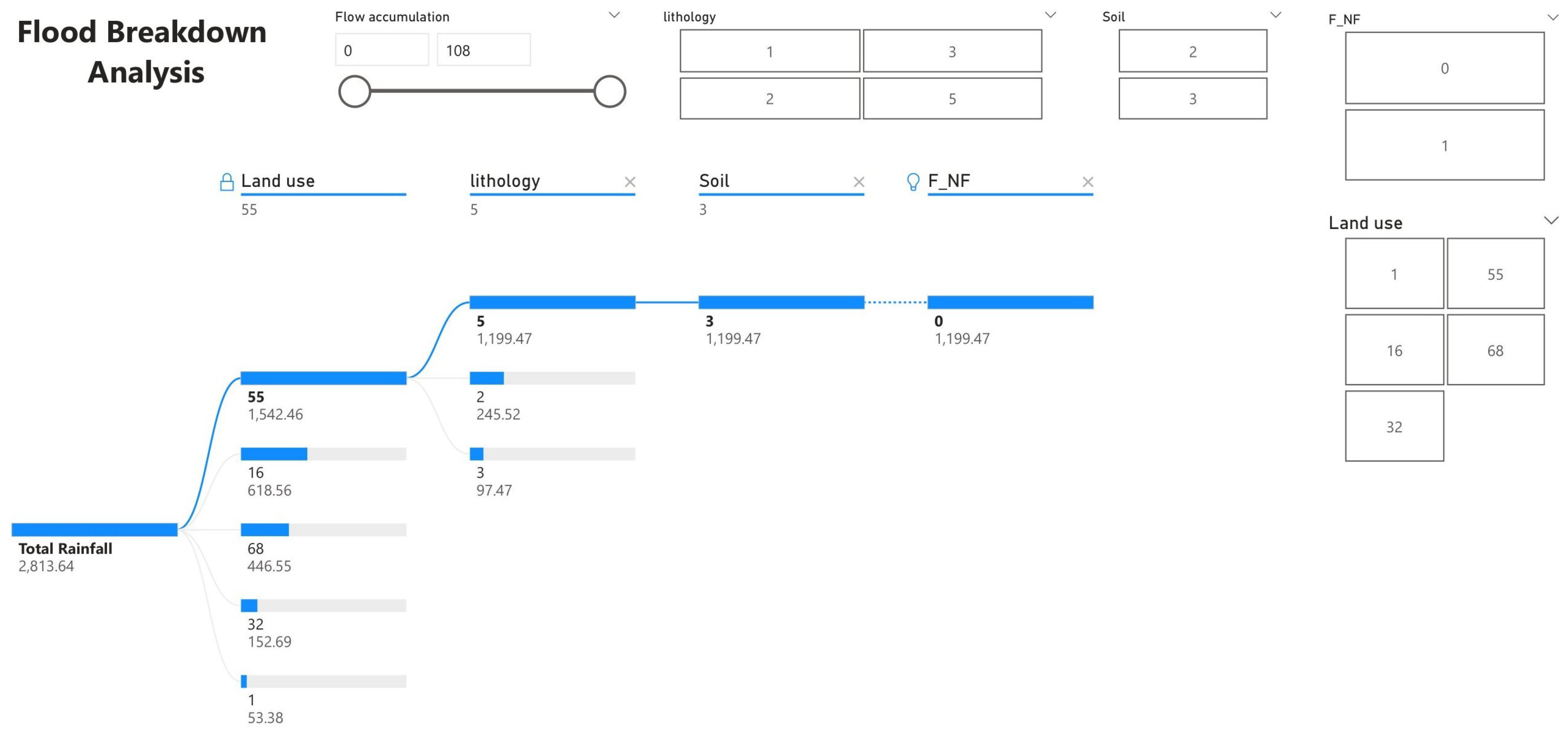
Figure 2 illustrates the analysis of the flood multifactor in detail. As shown in the right side of the figure for this graphical representation, two main classes, i.e., 0 and 1 for no flood and flood, respectively. The range is selected between minimum and maximum rainfall, i.e., 45.85 to 54.01. lithology plays a critical role in understanding the geology of a particular area. It has the potential for various geological hazards, including rainfall and flood. Therefore, four lithology classes are selected 1, 2, 3, and 5. Class number 4 represents sedimentary deposit, it covers only 1.1% of the total area, since it has little impact on flood formation therefore it was excluded.
Additionally, the selection of the Y factor is also shown on the right side. The graphs of the variable will vary according to the parameters selected in the Y-axis. The first graph shows the total rainfall by land use. The land use is divided into five sub-classes, and a different colour represents each class. The 5 classes are as follow:
Agriculture land represents to 1
Built Area represents to 16
Roads represent to 32
Mountains represent to 55
Bare land represents to 68
The data points lie near the correlation line, and the numbers of outliers are relatively low.
Similarly, the second graph shows the rainfall by flow accumulation and the sum of rainfall by soil. It is divided into two different classes. This graphical representation helps to calculate rainfall, its average, frequency, and valuable parameters. These parameters will assist in forecasting better results. The total rainfall is measured in millimetres. As the figure illustrates, the total rainfall is 2.81k mm. The average rainfall is calculated as 49.36k mm. Similarly, the minimum and maximum rainfall is 45.85k mm to 54.01k mm, respectively.
Figure 3 illustrates the correlation plot for the sum of rainfall and the average sum of rainfall. The majority of data points lie near the correlation line. This figure considers two main classes, i.e., flood and non-flood and total rainfall affected by lithology. Flood and non-flood are further divided into two sub-classes. The contribution of each class is illustrated in the doughnut chart. Similarly, four sub-classes of lithology, and the contribution of each class, are represented in the doughnut chart. These graphs are drawn by keeping TWI as a Y factor and the flow accumulation from 0 to 180.
Figure 4 shows the correlation analysis for the lithology class. The lithology class is divided into four sub-classes, and each class is denoted with different colors. The graph represents the clustering of sub-classes. It can be observed that blue and aqua-blue clusters dominated. The graph was drawn by keeping the profile and the plan curvature on the
x-axis and
y-axis, respectively.
The correlation plot in
Figure 5 represents the average sum of rainfall with respect to TWI and all the participating classes. The graph shows the clusters resulting when the sum of TWI decreases, with the rain tending to increase. Furthermore, for the given scenario, the sum of TWI decreased to 2.08. The flow accumulation was the same as that in the previous graph.
Figure 6 illustrates the breakdown of total rainfall. This breakdown shows that total rainfall is divided into four participating classes, these being land use, lithology, soil and FNF. The graph’s upper side shows the sub-classes with higher contributions, and the hierarchy descends to the classes with lower participation. Collectively, these classes help in calculating total rainfall and water value.
This study utilized dependency analysis because this is a well-known and efficient method in engineering and science. It is also considered an innovative method for forecasting precipitation and flood. In
Figure 7, the correlation between variables in the Jeddah dataset is depicted. A correlation matrix is a statistical tool that helps in understanding the relationship between different variables in a dataset. It measures the degree of association or correlation between pairs of variables. The correlation coefficient ranges from −1 to +1, where −1 indicates a perfect negative correlation, +1 indicates a perfect positive correlation, and 0 indicates no correlation between the variables. Correlation matrices are useful in data analysis, as they provide insights into the strengths and directions of relationships between variables, which can be used to guide further analysis or to inform decision making. According to the analysis, TWI, FA, SPI, and P directly correlated with the target parameters. In contrast, the remaining variables, such as TPI, TRI, DEM, aspect, PC, slope, lithology, soils, LU, and DR, exhibited an indirect correlation.
2.4. Proposed Methodology
A considerable number of algorithms have been applied to flood prediction in recent years. However, predicting which algorithm will work well in accordance with the region and weather conditions is challenging. The optimal algorithmic parameters for a particular problem need to be discovered, making it challenging to determine which parameters would yield the best results for a given algorithm. By conducting a comparative analysis of various algorithms, one can achieve more accurate predictions and obtain satisfactory results. This approach allows for a comprehensive evaluation of different algorithms’ performances in flood prediction. The modeling of the process is initiated by collecting data from different repositories. Categorical label data is generated after identifying the threshold above. After identifying features and corresponding labels, the dataset is partitioned into training and testing subsets. After training the model, several measures of evaluation are employed to validate the accuracy of the proposed model. Ultimately, the measurements are compared to the current models to determine the capability of the suggested model. The following subsection provides an overview of the implemented ML models, along with explanations of their corresponding performance indices.
2.5. Gradient Boosting Classifier
The gradient-boosting classifier acts as a sequential ensemble learning model in classification and regression problems. The algorithm can deal with complicated nonlinear correlations between input features and output variables, making it well-suited for predicting flood patterns based on various environmental factors. The model is presented so the previous base learner is always less effective than the existing base learner. It means the model improves its efficiency with each iteration. In the gradient boosting algorithm, the weights are not incremented in cases of misclassified outcomes. In other words, the model is not designed to add weights to misclassified results. Instead, it adds an adaptive model that appends the weak model and reduces the loss function. In this way, the loss function of the previous learner can be optimized. The primary objective of gradient boosting is to reduce the error rate of the previous classifier [
19].
Much research has been done to forecast floods with ensemble models and traditional algorithms. However, it is challenging to predict accurate outcomes irrespective of the dataset. Therefore, the central aim of this research is to propose a model that offers satisfying results across different types of data to forecast floods.
2.6. XGB Classifier
XGBoost is a software library developed by the Distributed Machine Learning Community (DMLC). Gradient Boosting (GB) is a machine learning technique that iteratively adds weak models to a robust model. The XGB and Gradient Boosting classifiers often work in an ensembled approach to offer satisfactory results and strengthen weak learners. However, XGB boosts the primary gradient boost with the help of an optimized system and improved algorithms. Chen et al. [
20] initially proposed XGB, which other developers further developed. It is a robust algorithm that combines the strengths of gradient boosting and decision trees, resulting in high accuracy and efficiency in predicting flood patterns. Initially, the data fits a relatively weak classifier. The current model’s performance is improved by further adding one more classifier, which is also weak in nature. However, this addition does not disturb the hierarchy if the previous classifier and the process continue. Each new classifier added looks for the positions where the previous classifier did not perform well. Both XGBoost and gradient boost are decision tree-based algorithms. Therefore, the performance of the algorithms is improved with the help of several tree-related hyperparameters, such as maximum depth and sub-samples. It also assists in reducing the overfitting problem. Furthermore, the learning rate parameter controls the weight assigned to each tree added to the model and affects the rate at which the model adapts to the training data.
2.7. Ada Boost Classifier
Adaptive boosting classifier belongs to the boosting family of algorithms. This algorithm focuses more on misclassified samples, adjusts the sample distribution and repeats the process until the weak classifier has been trained a predetermined number of times, completing the learning process. In the beginning, all the training samples are assigned similar weights. Incorrect predictions from the previous model are used to train the next classifier. The probability of selecting the correct error sample and the probability of selecting the paired sample decrease gradually. There is no chance of overfitting in Ada Boost. This is because the existence of test error independent of T. test error is lower when the margin in the training set is higher. The classification accuracy of the weak classifier used in AdaBoost is superior to random guessing, which has a probability of being correct of 0.5. However, Ada Boost’s performance in regard to noisy and abnormal data could be better. As a result, an increase in noisy data can lead to longer execution times and a decrease in algorithmic efficiency [
21].
2.8. LGBM Classifier
LGBM is known for its efficient handling of large datasets and high-speed training. Splitting computation is one of the significant differences between LightGBM and XGBoost. Gradient-based one-sided sampling (GOSS) helps identify the observation that is further used for splitting computation in LightGBM. XGBoost uses a histogram-based algorithm to select the relevant observations for the split. The efficiency of LightGBM is generally higher than XGB because the histogram-based algorithm offers more computation time than GOSS. Another point of differentiation between the two techniques is how they handle categorical features. Boost utilizes a one-hot encoding approach to convert categorical values to numeric ones while permitting users to specify the number of splits for a given categorical feature. LGBM also provides built-in support for categorical features, eliminating the need for one-hot encoding and improving the algorithm’s accuracy and training speed [
22].
2.9. Random Forest Classifier
The hierarchy of tree-based classifiers builds a random forest algorithm. Text data typically have many dimensions and irrelevant attributes in the dataset. However, only a few key attributes are actually informative for a classifier model. The most significant attributes from the dataset are selected in the random forest with the help of simple predetermined probability. Breiman developed the RF algorithm by utilizing subsets of sample data and constructing multiple decision trees by randomly mapping feature subspaces [
23]. The training data D and features N explain the random forest in the following ways: Predetermined probability helps in selecting D1, D2, D3,
… Dk.
Each document of training data denoted by DK is used to build a decision tree. The available features randomly sample the training documents using a subspace of the m-try dimension. M-try features help in calculating all possible probabilities. The optimal data split is found at the leaf node, and the process is repeated until the final iteration. The random forest ensemble combines a number of unpruned trees and takes a classification decision with a high probability value.
3. Results and Discussion
The results of these studies were carried out using GBC, XGBC, ABC, and LGBMC. The training and testing data were divided into an 80% to 20% ratio. All the evaluations of the suggested models were conducted in a Python programming environment with supporting libraries, such as pandas, sklearn neural network, and numpy models, and sklearn utils and metrics, among others. The model reads the dataset file initially, and then the data is directed towards training and testing. Training models were augmented along with the hyperparameters to tune for each model. In addition, GridSearchCV was used with cross-validation to obtain the results. This study achieved optimal parameters, including the number of iterations, prediction speed, and training time, for all classifiers and in selecting the best-stopping criteria. Multiple metrics were employed to assess the vulnerability of precipitation in the research area.
3.1. Model Evaluation Parameters
Several parameters were used to verify the suggested model’s efficacy, such as precision, sensitivity, specificity, and accuracy. Furthermore, performance evaluators were considered necessary if a spatial correlation existed between flood and non-flood areas and the forecast flood-prone zone.
Accuracy: This measured the overall correctness of the model’s predictions. It is the ratio of the number of correct predictions (true positives values (TPV) + true negatives values (TNV)) to the total number of predictions, as shown in Equation (
1). Precision: This measured the proportion of true positive predictions among all positive predictions made by the model. It is the ratio of the number of true positives to the total number of positive predictions (TPV+ false positives values (FPV)), as depicted in Equation (
2).
Recall: This measured the proportion of true positive predictions among all actual positive cases in the data. It is the ratio of the number of true positives to the total number of actual positive cases (TPV + false negatives values FNV), as shown in Equation (
3). F1-Score: This is the harmonic mean of precision and recall, and it provides a balanced view of both metrics. It is the weighted average of precision and recall, where the weights are determined by the beta value. In this case, the beta value was set to 1, which gave equal importance to both precision and recall, as described in Equation (
4).
Furthermore, the error rate of the flood susceptibility was calculated using the root mean squared error (RMSE), coefficient of determination (R
), mean squared error (MAE), and mean absolute error (MAE), mean absolute percentage error (MAPE). Their mathematical equations are presented in Equations (5)–(9).
where
represents the acutal value,
is the predicted value, and K represent number of observations.
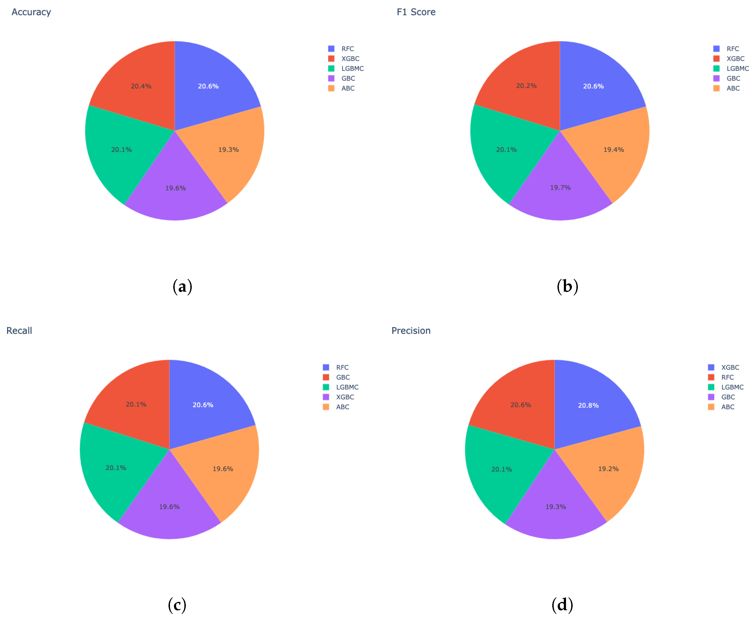
The pie chart in
Figure 8a displays the accuracy of five different algorithms, namely RFC, XGBC, LGBMC, GBC, and ABC. Each algorithm is represented by a different color in the pie chart. The algorithm with the highest accuracy of 20.6%, RFC, is represented by the largest area of the pie chart. XGBC had the second-highest accuracy, represented by 20.4% of the pie chart. LGBMC, GBC and ABC are covered by 20.1%, 19.6%, and 19.3% of the pie chart area. Overall, the pie chart provides a clear visual representation of the relative accuracies of the five algorithms. Similarly, in
Figure 8b, the pie chart displays the F1 score of five different algorithms, namely RFC, XGBC, LGBMC, GBC, and ABC. The algorithm with the highest F1 score or 20.6%, RFC, is represented by the largest area of the pie chart. XGBC had the second-highest F1 score, represented by 20.4% of the pie chart. LGBMC, GBC and ABC had scores of 20.1%, 19.7%, and 19.4%, respectively, as reflected in the corresponding pie chart areas.
Figure 8c displays the recall of the proposed algorithms. The algorithm with the highest recall, RFC, is represented by the largest area of the pie chart, with a score of 20.6%. XGBC and LGBMC had the second-highest recalls, represented by 20.1% of the pie chart. GBC and ABC had recalls of 19.6% each, as seen in the pie chart areas.
Figure 8d shows the precision values of the proposed algorithms. The algorithm with the highest precision of 20.8%, XGBC, is represented by the largest area of the pie chart, RFC had the second-highest precision, represented by 20.6% of the pie chart. LGBMC, GBC and ABC cover 20.1%, 19.3%, and 19.2% of the pie chart area, respectively.
Figure 9 is a line graph depicting the accuracy, F1 score, precision, and recall values of the proposed algorithms. The graph provides an insightful comparison of how the proposed algorithms performed across various evaluation metrics. From the analysis, it is evident that RFC and XGBC were relatively high performers compared to the other algorithms, consistently producing high scores across all the metrics. The accuracy and F1 score values, for all the proposed algorithms, ranged from 0.80 to 0.87, reflecting good overall performance. The recall values, on the other hand, ranged from 0.88 to 0.94, indicating that the algorithms were effective in identifying and classifying the relevant data points. However, the precision value ranged from 0.75 to 0.81 in all algorithms, highlighting that there were instances where the algorithms classified non-relevant data points as being relevant. Overall, the results from the line graph suggest that the proposed algorithms are capable of achieving high performance across various evaluation metrics, with some performing relatively better than others.
3.2. Flood Susceptibility Map
Some places are prone to floods, such as Jeddah. Historical data was used to make flood susceptibility maps. Different methods were used to categorize and analyze the data. One standard method is the quantile-based approach. It helps to show which areas are most at risk of flooding. It was found that some areas near the river were more likely to flood than others.
Figure 10 provides the proposed flood susceptibility graph. In order to compare the results of flood-prone areas, the study utilized bivariate and univariate statistical results. Our findings suggested that areas near western catchments with high TWI and DR were more likely to experience floods.
Additionally, the study observed that, even with a low frequency of occurrence, the topography of a few watershed areas is prone to flooding. A flood susceptibility graph with evaluation parameters (low, very low, moderate, high, and very high) and 39 degrees 20 min East longitude provides a visual representation of the results, making a comparison of the performances of different proposed algorithms easier. The x-axis shows the different algorithms used to evaluate flood susceptibility, each algorithm being assigned a specific value. The y-axis displays the level of flood susceptibility.
An evaluation of the proposed model’s performance was conducted through a comparative analysis. In this context, some studies from the literature were collected based on their having similar performance evaluations to those used in the suggested model as shown in
Table 1. In [
24], the authors utilized four algorithms, as stated in the table. Random forest outperformed the KNN, Decision Tree and SVM in accuracy, precision and recall matrix. The study did not add the score of sensitivity to the results. Therefore, there is room for improvement, as the results of the algorithms could be more satisfactory.
In [
25], decision tree, random forest, naive Bayes and neural network were proposed. The decision tree outperformed the naïve Bayes, neural networks and random forest in terms of precision, recall, and senstivity values. However, the accuracy value was not computed. As compared to our proposed model, we achieved better results in terms of precision, recall, and sensitivity values.
In [
26], the MLP had relatively good performance in comparison to KNN and Decision tree for precision and sensitivity values. In terms of recall, KNN achieved higher values. The study considered two classes, Rain and No Rain, for generating the results. The classification matrices results were not satisfactory. Based on the results, the model could not be used in real time systems.
Similarly, in [
27], the authors considered artificial neural networks and support vector machines to generate results for forecasting rain. The accuracy of ANN was comparatively high compared to SVM. However, the study did not explain the recall score of the utilized algorithms. In contrast, the proposed work achieved better results in term of classification matrices.
In [
28], the authors utilized BE-C2, LT-C2, k-SVM-C2, and KNN-C2 to evaluate their model’s performance in forecasting floods in Jeddah, the Kingdom of Saudi Arabia. LT-C2 offered the maximum accuracy at 69%, and the lowest performing algorithm was KNN-C2, with a 65% accuracy rate. It is worth noting that there was a slight discernible variance in the performance values between the best performing and worst performing algorithms. This illustrated that there was margin for improvement in performance. The proposed study overcame this shortcoming by offering satisfactory results.
Similarly, the suggested model utilized five machine learning algorithms to predict a flood. The table shows that, unlike other models in the same domain, the suggested model of boosting classifiers and random forest achieved the top results for precision, recall, f1-score, and accuracy.
Table 2 illustrates the regression results for the proposed model. The first column explains all the utilized machine learning regressors, while the remaining columns show the regression matrices. In terms of error values, all regressors performed exceptionally well by securing error values near to zero. In MAPE, the average absolute percentage error between the predicted values and the actual values were calculated. The work presented had a higher MAPE value, considered an average result. The R-squared values ranged from 0 to 1, with higher values indicating a better fit between the model and the data. If the R
value is greater than 0.5, it is considered a good result. Gradient and extreme gradient boosting regressors have shown the most satisfactory results as their values are closer to zero. Therefore, the lower values explain that the model is trained perfectly.
Gradient Classifier and Random Forest Classifier exhibited the best performances across all evaluating criteria. The precision, recall, f1-score and accuracy values were impressive. The success rate of the suggested model makes it a better choice over other models for forecasting floods.
4. Conclusions
This study demonstrates that machine learning algorithms, namely GBC, XGBC, ABC, LGBMC, and RFC, show exceptional performance in predicting flood and non-flood regions in Jeddah, Saudi Arabia dataset. Specifically, the accuracy values ranged from 82% to 86%, with RFC achieving the highest performance among all the models. In terms of precision, the values ranged from 75% to 82%, with RFC once again outperforming the other models. The recall values ranged from 89% to 91%, with RFC and LGBMC exhibiting the best performances. Similarly, the sensitivity values ranged from 81% to 86%, with RFC again outperforming other models. The error rates of the proposed algorithms were also considered, with MSE ranging from 0.007 to 0.009, MAE ranging from 0.06 to 0.07, RMSE ranging from 0.086 to 0.095, MAPE ranging from 31.714 to 34.299, and R ranging from 0.518 to 0.597. Utilizing machine learning algorithms with the help of regression matrices can significantly enhance flood prediction accuracy, enabling informed decision-making in diverse industries and sectors. However, the study is limited by the small dataset used for the model. Future research can further refine the models to make them more effective in predicting floods in different regions and under different weather conditions. Despite this limitation, the suggested model can serve as a promising alternative to spatial flood forecasting models.

 ,
, 


