Article

Stable Isotope Signatures in Tehran’s Precipitation: Insights from Artificial Neural Networks, Stepwise Regression, Wavelet Coherence, and Ensemble Machine Learning Approaches

by
Mojtaba Heydarizad
1,
Luis Gimeno
2,*,
Masoud Minaei
3,4 and
Marjan Shahsavan Gharehghouni
3
1
State Key Laboratory of Marine Geology, Tongji University, Shanghai 200092, China
2
Centro de Investigación Mariña, Environmental Physics Laboratory (EPhysLab), Campus As Lagoas s/n, Universidade de Vigo, 32004 Ourense, Spain
3
Department of Geography, Ferdowsi University of Mashhad, Mashhad 9177794883, Iran
4
Geographic Information Science/System and Remote Sensing Laboratory (GISSRS: Lab), Ferdowsi University of Mashhad, Mashhad 9177794883, Iran
*
Author to whom correspondence should be addressed.
Water 2023, 15(13), 2357; https://doi.org/10.3390/w15132357
Submission received: 7 May 2023 / Revised: 18 June 2023 / Accepted: 23 June 2023 / Published: 26 June 2023
(This article belongs to the Special Issue The Use of Environmental Isotopes in Hydrogeology)

Abstract

:
This study investigates the impact of precipitation on Middle Eastern countries like Iran using precise methods such as stable isotope techniques. Stable isotope data for precipitation in Tehran were obtained from the Global Network of Isotopes in Precipitation (GNIP) station and sampled for two periods: 1961–1987 and 2000–2004. Precipitation samples were collected, stored, and shipped to a laboratory for stable isotope analyses using the GNIP procedure. Several models, including artificial neural networks (ANNs), stepwise regression, and ensemble machine learning approaches, were applied to simulate stable isotope signatures in precipitation. Among the studied machine learning models, XGboost showed the most accurate simulation with higher R2 (0.84 and 0.86) and lower RMSE (1.97 and 12.54), NSE (0.83 and 0.85), AIC (517.44 and 965.57), and BIC values (531.42 and 979.55) for 18O and 2H compared to other models, respectively. The uncertainty in the simulations of the XGboost model was assessed using the bootstrap technique, indicating that this model accurately predicted stable isotope values. Various wavelet coherence analyses were applied to study the associations between stable isotope signatures and their controlling parameters. The BWC analysis results show coherence relationships, mainly ranging from 16 to 32 months for both δ18O–temperature and δ2H–temperature pairs with the highest average wavelet coherence (AWC). Temperature is the dominant predictor influencing stable isotope signatures of precipitation, while precipitation has lower impacts. This study provides valuable insights into the relationship between stable isotopes and climatological parameters of precipitation in Tehran.

1. Introduction

Tehran, the capital of Iran, is the most populated and largest metropolitan area in the country. Over the last few decades, the water shortage crisis has significantly affected the lives of millions of people living in this city. Therefore, assessing the conditions of existing water resources and discovering new ones is critical for this metropolitan area. Stable isotope techniques play a crucial role in the study of precipitation because of their accuracy and the simplicity of their application in water resource studies. In water resource studies, the assessment of precipitation characteristics is an important initial step. Many studies [1,2,3,4,5,6,7] in Iran have used stable isotope techniques, such as precipitation moisture identification, to assess precipitation characteristics. The Global Network of Isotopes in Precipitation (GNIP) has established a global network of stations in order to sample and analyse stable isotopes in precipitation. GNIP only had one “Tehran” station in Iran, which covered an area of over 1,648,195 km2. This station was operational from 1961 to 1987 and again from 2000 to 2004. In addition to stable isotopes (18O and 2H), precipitation samples at this station were analysed for 3H.
The stable isotope content of precipitation is controlled by local factors (such as air temperature, precipitation amount, and water vapour pressure) and regional components (teleconnection indices). Some of these teleconnection indices’ effects on precipitation stable isotope signatures have been studied in surveys worldwide, including [8,9,10,11,12,13]. Among the various teleconnection indices, only bivariate ENSO (BEST), southern oscillation index (SOI), North Atlantic oscillation (NAO), Indian Ocean dipole (IOD), and quasi-biennial oscillation (QBO) have an impact on Iran [14,15,16,17,18].
Isotope simulation can help to improve hydrological modelling in areas where there are not enough precipitation sampling stations to measure the stable isotope signature of precipitation. To simulate stable isotope signatures in precipitation, precise techniques such as statistical techniques can be used. Stepwise regression models are among the most accurate simulation methods. These models use both local and regional parameters as predictors to simulate the target variable (stable isotopic signatures of precipitation). Stepwise regression is a technique for building regression models where the selection of predictors is conducted automatically. This method involves iteratively evaluating the statistical significance of each predictor in a linear regression model. Forward selection, backward elimination, and bidirectional elimination are three approaches to stepwise regression. In the backward approach, the stepwise method starts with a full model containing several predictors and then removes one predictor at a time to test the importance of each. In contrast, the forward selection approach begins with no predictors and adds them one by one, testing for statistical significance at each step. Finally, bidirectional elimination combines both the backward and forward methods to determine which predictors should be included or excluded from the model [19,20]. The stepwise technique has several advantages, including its high accuracy and speed compared to other statistical models. Additionally, this model can identify the most effective predictors influencing the target variable, which is crucial when there are many predictors. However, the main disadvantage of the stepwise model is that it can lead to data overfitting. This means that the stepwise model may fit the data with high accuracy, capturing even the random noise in the data, and in addition determine the relationship between the predictors and target variables [21,22]. Stepwise techniques have been applied in some climate studies at several sites across Iran and the Middle East. For example, Mohammadzadeh and colleagues used the stepwise technique to study and simulate the stable isotope signature in precipitation in western Iran and eastern Iraq [23]. Heydarizad and colleagues used stepwise techniques to study the stable isotope signature in precipitation and groundwater resources across Iran. They presented maps of the spatial distribution of 18O, 2H, and d-excess in precipitation across Iran using the stepwise technique [4]. Additionally, Heydarizad and colleagues developed a spatial distribution map of stable isotope signatures in precipitation across the Middle East using the stepwise model [24].
Advanced machine learning techniques (ML) can also predict stable isotope signatures in precipitation. Artificial neural network (ANN) techniques [25,26] are among the most widely used ML models in a variety of scientific fields. McCulloch and Pitts developed an ANN technique in 1943 by creating a computational model for neural networks [27]. A deep neural network (DNN) model contains several hidden layers between the predictors and target variables, as opposed to comprising a simple black-box shallow neural network (SNN) model with only one hidden layer. The DNN model can be applied to cases where the predictor and targets variables have highly comprehensive and complex relationships. The term “deep” in deep learning is due to the application of multiple layers in the network. A multi-layer perceptron (MLP) is a common subset of DNN. An MLP is made up of units known as perceptrons. These have one or more inputs, with an activation function and an output. An MLP model is constructed by arranging perceptrons in structured layers. The perceptrons in a given layer are independent of each other but are connected to all other perceptrons in the next layer. Each layer consists of a set of neurons and is trained using a backpropagation algorithm. Backpropagation is one of the most widely used algorithms for the supervised training of multilayer neural networks [28]. It works by approximating the nonlinear relationship between the input and output by adjusting the internal weight values [29]. Artificial Neural Networks (ANNs) have several advantages, including their ability to work with large datasets and to identify complex patterns between predictors and the target parameter. Additionally, the multiple hidden layers in Deep Neural Networks (DNNs) increase their efficiency at learning complex features and performing more complicated computational tasks [30]. In Iran, Deep Neural Networks (DNNs) have been applied to hydrology and climatology in several studies. For example, Sahour and colleagues used a DNN to model the salinity of groundwater due to seawater intrusion into coastal aquifers in the Caspian Sea region. [29]. Heydarizad and colleagues examined the primary sources of moisture that contribute to precipitation in Iran using the FLEXPART model and predicted precipitation amounts by employing moisture uptake rates as predictors with various machine learning techniques, including DNNs [31]. Dehghani and colleagues employed a multi-layer feed-forward artificial neural network (FFANN) to predict hydrological drought in the Karoon River in southwestern Iran using the Standardized Hydrological Drought Index (SHDI) time series [32]. Hamidi and colleagues contrasted support vector machines (SVMs) and artificial neural networks (ANNs) in their ability to model monthly precipitation fluctuations at two synoptic stations in Hamadan, Iran [33]. ANNs have also been used to simulate the stable isotope signatures of precipitation. Heydarizad and his colleagues have used an ANNs to predict the stable isotope signatures in precipitation in Bangkok. They investigated the role of local (wind speed, potential evaporation, vapor pressure, air temperature, and precipitation amount) and regional parameters (teleconnection indices) on the stable isotope content in the precipitation. Their study demonstrated that among the local and regional parameters, precipitation amount and potential evaporation (local) and the BEST teleconnection index (regional) had dominant roles in controlling the stable isotope content of the precipitation [13].
In addition to neural networks, other machine learning techniques such as ensemble learning models, including extreme gradient boosting (XGBoost) and Random Forest (RF), have also been applied in water resources studies, including isotope hydrology. XGBoost is an ensemble learning method that uses multiple decision trees to make predictions. It is based on the principle of gradient boosting, which improves the performance of a model by iteratively adding new models to the ensemble. Each new model is trained to correct the errors made by the previous models. XGBoost uses a more regularised model formalization to control over-fitting, giving it better performance compared to other gradient boosting techniques. It also has several other features that make it efficient and effective, such as handling missing values and parallel processing. XGBoost has been widely adopted in data science competitions and real-world applications due to its high performance and versatility [34]. This method has been applied in some studies to predict the stable isotope signatures in precipitation. For example, Nelson and his colleagues used XGboost to simulate the stable isotope signatures in precipitation at a monthly resolution across Europe. Their model predictions are accurate enough to be applied for exploration of inter-annual and long-term variability of both stable isotopes (18O and 2H) in water resources across Europe [35]. In another study, the stable isotope content in precipitation was simulated using geostatistical and machine learning methods. Their results showed that machine learning techniques performed better compared to geostatistical models [36]. RF is another ensemble learning method that operates by constructing a multitude of decision trees at training time and outputting the class that is the mode of the classes (classification) or mean prediction (regression) of the individual trees. This algorithm is known for its ease of use and flexibility in handling both classification and regression problems. In a study by Erdelyi and colleagues, they compared the performance of different variants of RF in predicting the spatial variability of precipitation stable oxygen isotope values across Europe. The developed models were evaluated based on their ability to reproduce overall trends and seasonal patterns of precipitation stable isotope variability. The results showed that all variants were capable of reproducing these trends and patterns, with the RFsp model yielding the smallest mean absolute error and highest Lin’s concordance correlation coefficient [37].
The current study has two main goals. Firstly, it aims to study the impacts of local and regional parameters on stable isotope signatures of precipitation. Secondly, it aims to simulate the stable isotope signatures in Tehran Metropolitan precipitation using various regression techniques, including stepwise model, ANNs, RF, and XGboost. The accuracy of the developed models has been assessed using various methods, and the most accurate model has been selected among the studied ones. Finally, Bootstrap uncertainty analysis has been used to estimate the uncertainty in the most accurate developed model. In the second step, wavelet coherence analysis has been used to characterize the dynamic relationship between the studied datasets.
In this study, we aim to provide an in-depth examination of stable isotope signatures in Tehran’s precipitation through the application of ANNs, stepwise regression, XGBoost, RF, and wavelet coherence methodologies. Our research question is: How can we accurately simulate the stable isotope signatures of precipitation in Tehran using various machine learning models? To answer this question and achieve our objectives, we collected and pre processed data, selected relevant input data, chose appropriate machine learning algorithms or statistical models, trained and evaluated our models using appropriate metrics, performed cross-validation, chose the best-performing model, performed uncertainty analysis, and used bivariate wavelet coherence (BWC) and partial wavelet coherence (PWC) analyses to study the correlation between predictors and target value. This study is innovative because it is the first to simulate the stable isotope signatures of precipitation in the Middle East region and Iran using various machine learning models and to consider the role of different machine learning methods in simulating the stable isotope signatures of precipitation. Additionally, several methods were employed to select the best model and bootstrap uncertainty analysis was conducted on the most accurate model.
The remainder of this article is structured as follows: In Section 2, we describe the climate and topography of Tehran. In Section 3, we present our materials and methods, including data collection and pre processing, the selection of relevant input data, the choice of machine learning algorithms or statistical models, and the evaluation of our models using various evaluation metrics. In Section 4, we discuss the results of our analysis, including the performance of our models and the results of our uncertainty analysis as well as present our wavelet coherency analysis using BWC and PWC. Finally, in Section 5, we conclude the implications of our findings.

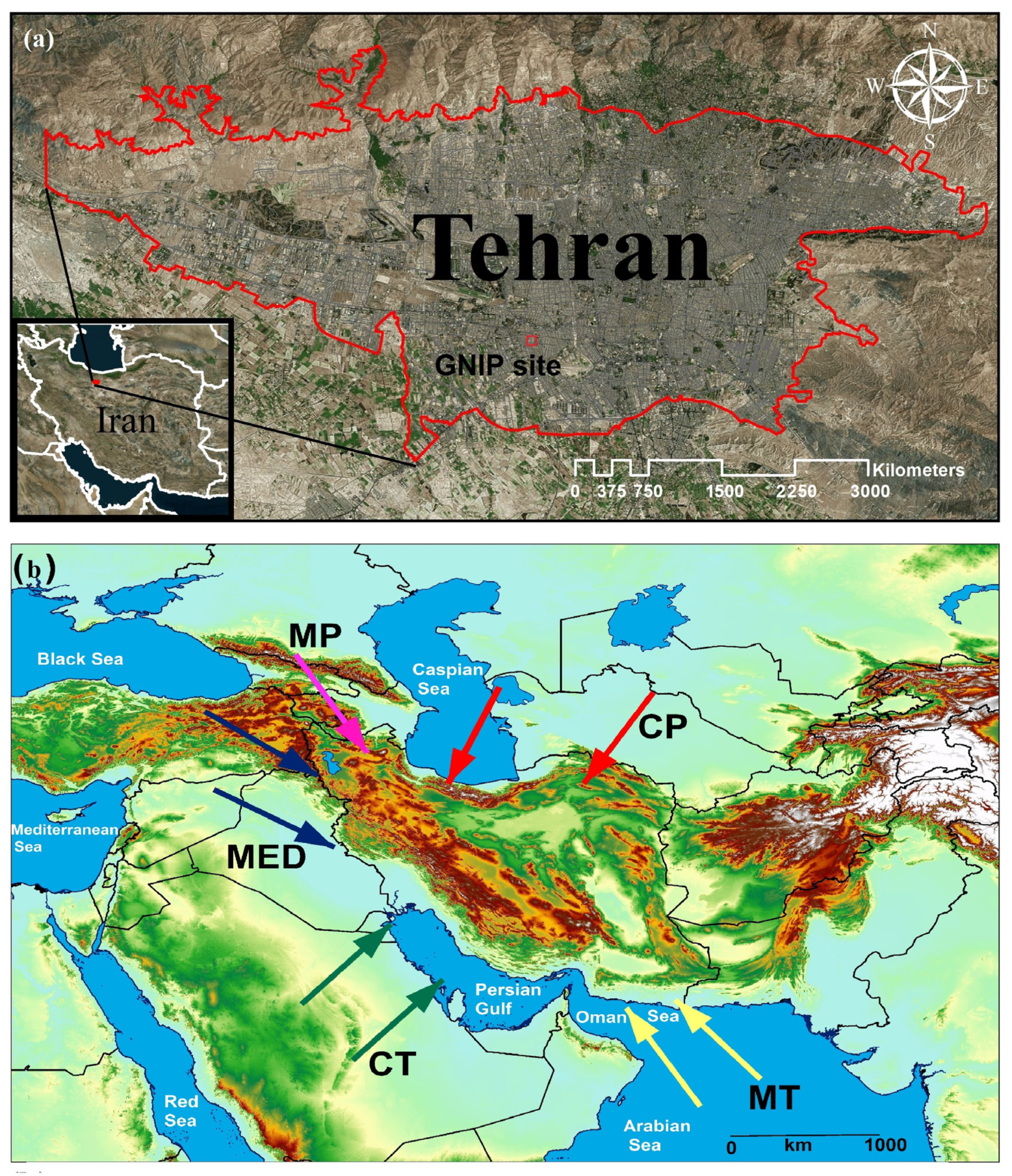
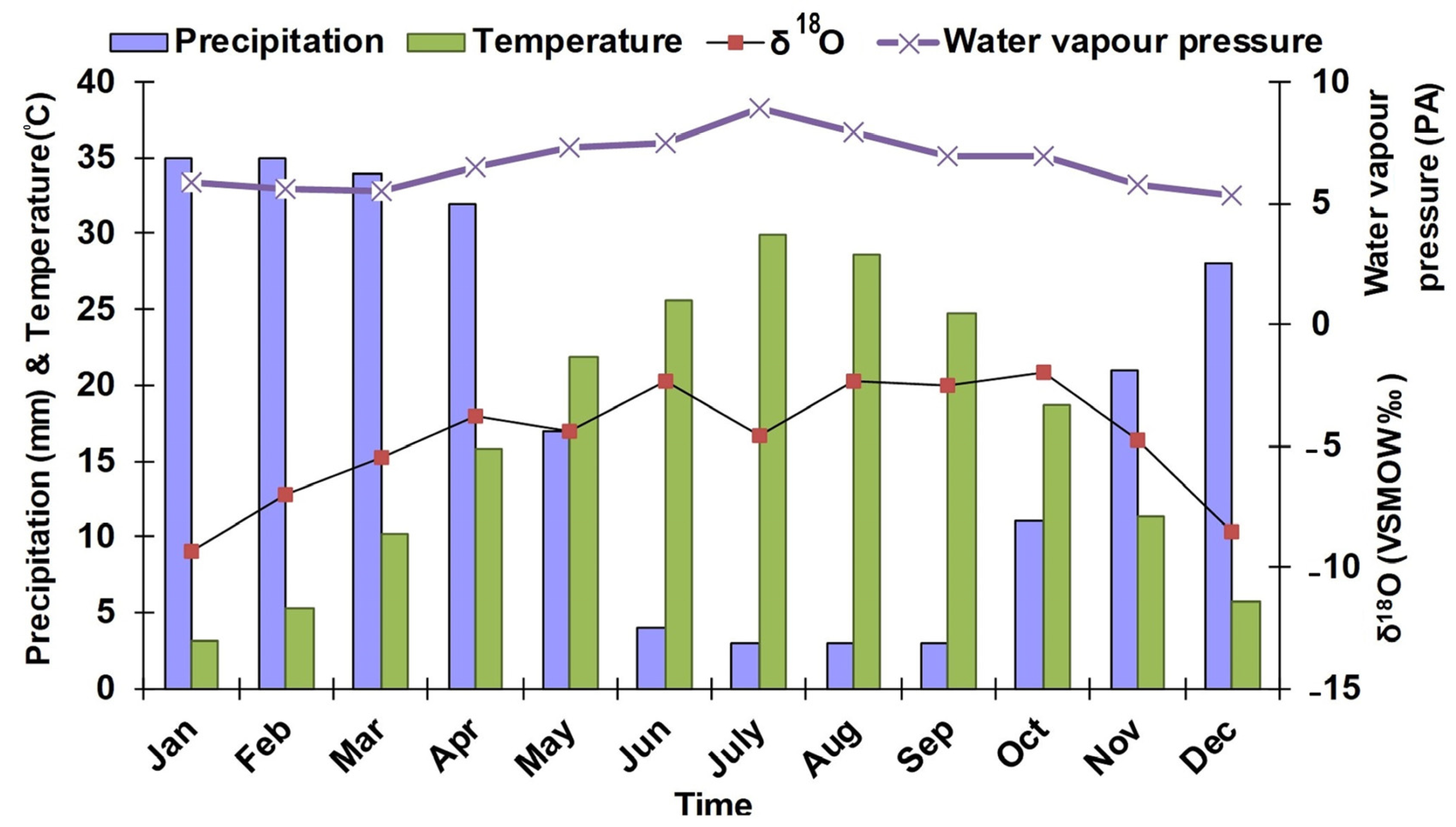
2. The Climate and Topography of Tehran

Tehran, Iran’s capital, has a population of over nine million people. It is the most populous metropolitan area in West Asia, and the Middle East’s most populous metropolitan area (Figure 1a).
The Köppen climate classification places Tehran in the BSk group with a cold semi-arid climate [24]. Tehran’s climate is heavily influenced by the geographic features that separate the city’s northern (Alborz Mountains) and southern (central desert) halves. Mount Damavand located near Tehran, has the highest elevation in Iran and even the Middle East region. The weather in Tehran is normally mild during spring and autumn. However, extremely cold and wet weather conditions occur in the winter, and hot and dry weather occurs during summer [22]. The monthly variations in some climatological parameters, including precipitation amount, air temperature, and water vapour pressure at the Tehran GNIP station, as well as stable isotope signatures in precipitation, are presented (Figure 2). During the cold period (November to April), the monthly precipitation amount showed higher values, while the water vapour pressure and air temperature showed lower values, compared to the warm period (May to October) of the year. The stable isotope signatures demonstrated depleted precipitation during the wet period. This was caused by rainout, which occurred as a result of more intense precipitation events (precipitation amount effect). However, enriched stable isotope values were observed during precipitation events in the warm and dry periods of the year. The dominant enrichment observed in the stable isotope signatures of precipitation during this period was caused by the negligible relative humidity in the atmosphere and high air temperature [38].
Large variations in monthly wind speed and direction, as well as precipitable water over Iran for the wet and cold as well as warm and dry periods, were observed (Figure 3). During cold and wet periods, moisture fluxes from the Persian Gulf, Mediterranean Sea, Arabian Sea, and Caspian Sea are observed toward Iran. The precipitable water also demonstrated higher values in the western and southwestern parts of Iran over the Zagros Mountains as well as in the Caspian Sea coastal area (Figure 3). However, during the dry period in northwestern Iran, precipitable water is primarily controlled by moisture originating from the Black Sea. Furthermore, moisture from the Caspian Sea has a strong influence on precipitable water in the Caspian Sea coastal area. The tropical monsoon causes massive wind systems and moisture transfer in the Indian Ocean and Arabian Sea. This tropical monsoon occasionally influences the southwestern part of Iran and causes large precipitation events (Figure 3). During cold and wet periods Tehran, receives a significant portion of its precipitation from Mediterranean, Maritime Polar (MP), Continental Tropical (Ct), and Continental Polar (CP) air masses. However, monsoon precipitation sometimes influences the southeastern part of Iran via Maritime Tropical (MT) air mass during the dry and hot periods (Figure 1b).

3. Materials and Methods

During this investigation, stable isotope data for precipitation in Tehran were obtained from the GNIP station located in 35°40′48″ N and 51°19′12″ E at an elevation of 1200 m [39]. Stable isotope signatures in precipitation of Tehran have been sampled for two periods: 1961 till 1987 and 2000 till 2004 on a monthly basis. The statistical characteristics of the studied parameters were analysed and are presented in Table 1.
The procedure for precipitation sampling for stable isotope analysis presented by GNIP has been used in this study [40].. After it rained, the precipitation samples were immediately transferred from the rain gauges into 1 L air-tight high-density polyethylene bottles to reduce evaporation. The bottles were then stored in a refrigerator, eliminating the need for additional substances like paraffin. The rain gauges were designed to resist evaporation and accurately measure precipitation amount. At the end of each month, the precipitation in the monthly bottles was shipped to a laboratory for stable isotope analyses.
Stable isotopes in precipitation samples have been analysed in several laboratory across the world including the university of Copenhagen (Denmark), International Atomic Energy Agency (IAEA), and AGH- University of Science and technology (Krakow, Poland) using a Los Gatos Research (LGR) Liquid Water Isotope Analyzer or a Delta-Plus XP isotope ratio mass spectrometer (IRMS) (Thermo Finnigan, Germany). The laboratories calibrated their stable isotope measuring instruments with VSMOW (Vienna Standard Mean Ocean Water) to avoid errors. Precipitation’s stable isotope values are expressed in delta notation (δ), which represents the sample’s relative deviation from the Vienna Standard Mean Ocean Water (VSMOW) and is determined using Equation (1):
δ = 1000 (RSample − RVSMOW)/RVSMOW
In this case, R represents the ratio of either 2H/H or 18O/16O. For the majority of samples, the analytical standard uncertainties were ±0.1 ‰ for δ18O and ±1 ‰ for δ2H.

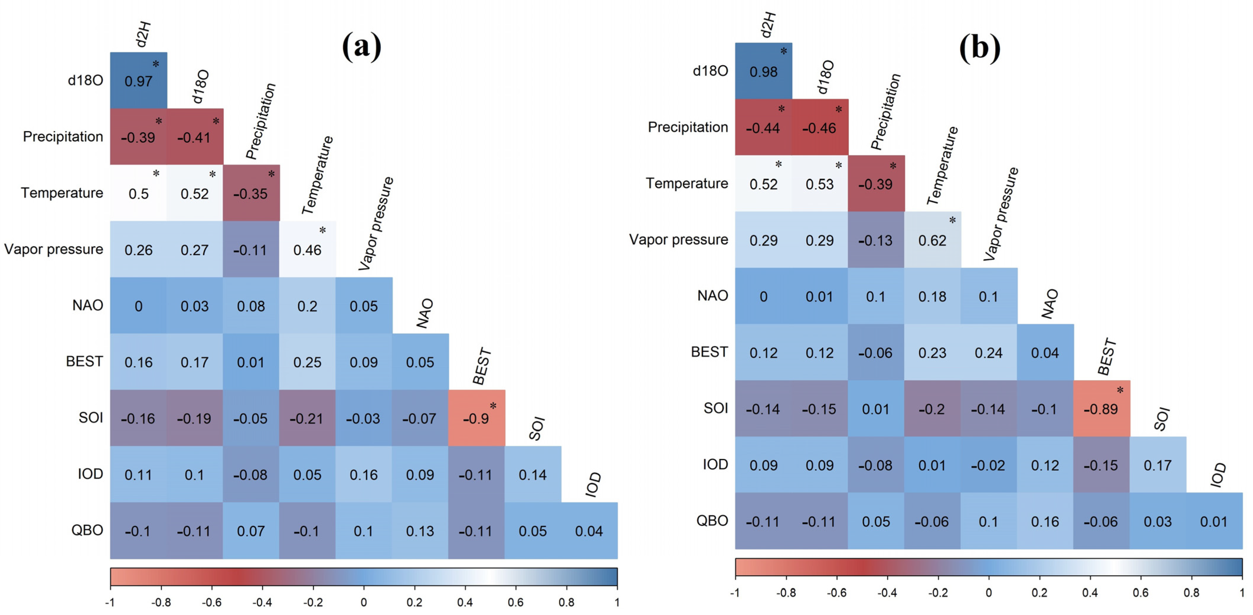
3.1. Selection of Predictors for Stable Isotope Simulation

In this stage, Local parameters such as precipitation amount, air temperature, and water vapor in Tehran were obtained from the GNIP network, while regional parameters including IOD, NAO, BEST, SOI, and QBO teleconnection indices were obtained from the National Oceanic and Atmospheric Administration (NOAA) website [41].

3.2. Simulation Models Applied to Predict Stable Isotopes Content

In this stage, the simulation models applied to predict stable isotope content are described. Several models were developed, including stepwise regression, ANNs (including DNN and SNN), XGBoost, and RF. Stepwise modelling is a useful tool for developing statistical models that accurately predict outcomes or responses while minimizing the number of predictors required [4,19,20,24]. This technique is used to choose the most suitable predictor variables for a multiple linear regression model, which is generally expressed as Equation (2):
y = β0 + β1x1 + β2x2 + … + βkxk + ϵ
where y represents the dependent variable, x1, x2, …, xk are the independent variables, β0, β1, β2, …, βk are the coefficients for the independent variables, and ϵ is the error term.
In addition to the stepwise technique, more advanced machine learning techniques, including ANNs, RF, and XGboost, have been applied. The ability of ANNs to automatically identify and extract features from input data is one of their primary advantages. ANNs, as opposed to traditional statistical models, can learn features directly from the input data. A simple shallow artificial neural network (SNN) with only one hidden layer and a deep neural network (DNN) were used to predict the stable isotope signatures of precipitation. To apply ANNs, it is highly important to have sufficient amount of data to train the model and to select appropriate neural network architecture that is capable of accurately representing the problem being simulated [42]. For the DNN model, the main parameters were as follows: The number and size of the hidden layers were specified by the ‘hidden’ parameter, which was set to two hidden layers with 150 neurons each. The number of training epochs was specified by the ‘epochs’ parameter, which was set to 5000. The activation function used was specified by the ‘activation’ parameter, which was set to ‘Rectifier’. However, for the SNN model, there was only one hidden layer. The main parameters were as follows: The number of units in the hidden layer was specified by the ‘size’ parameter, which was set to 150. The maximum number of iterations for the optimization algorithm was specified by the ‘maxit’ parameter, which was set to 5000.
In addition to ANNs, the RF model has also been applied to simulate the stable isotope signatures in precipitation. Similar to neural network techniques, certain requirements must be met to use RF. In RF model, a well-defined problem with labeled data will be needed to train the model [43]. The data should have some actual signal in the features so that the model can perform better than random guessing would, and it is also important to have a sufficient amount of data to train the model [44]. For the RF model, we used the train function from the caret package to train our model. The main parameters used were as follows: the model type was specified by the ‘method’ parameter, which was set to ‘rf’ for random forest. The performance metric used was specified by the ‘metric’ parameter, which was set to ‘accuracy’. The tuning grid for the hyperparameters was specified by the ‘tuneGrid’ parameter, which was set to a grid of values for the mtry parameter ranging from 1 to 10. The resampling method used for model selection was specified by the ‘trControl’ parameter, which was defined by the trControl object. The computation of variable importance was specified by the ‘importance’ parameter, which was set to TRUE. The minimum size of terminal nodes was specified by the ‘nodesize’ parameter, which was set to 14. The number of trees growing was specified by the ‘ntree’ parameter, which was set to 300. In addition, the data should have some actual signal in the feature so that the model can perform better than random guessing. Finally, the basic requirements for using both random forest and XGBoost are similar. However, there are some differences between these two algorithms in terms of their implementation and the specific details of how they work. For instance, XGBoost is based on gradient boosting, while RF is based on bagging. This means that there may be some differences in terms of the hyperparameters that need to be tuned and the specific techniques used to improve the performance of the model [45]. For the XGBoost model, a max_depth of 9, an eta of 0.1, a rate_drop of 0.01, a skip_drop of 0, a min_child_weight of 12, a subsample of 0.85, a colsample_bytree of 0.9, and a gamma of 5 were used. The objective was set to reg: linear and the eval_metric was set to rmse. The number of rounds for tuning was set to 1500.

3.3. Repeated v-Fold Cross-Validation

After creating the model with the help of training the data, its accuracy is evaluated by using the best dataset. To validate the machine learning methods, a common technique called cross-validation (v-fold variant) using rsample package in R language is used, which involves dividing the datasets in training and testing sets. The crucial concern when dividing data into training and testing sets is that the distribution of the test datasets may not be representative of the entire dataset [46]. In v-fold verification, the dataset is randomly partitioned in the v non-overlapping splits or subsets to divide data into training and test sets. Each split i (1 ≤ i ≤ v) is used as a validation set, while the model is trained on all other splits except for i. This process is repeated v times to ensure that every split is exactly once as a validation set [46]. A common approach is to use 5 or 10 repetitions of V-fold cross-validation, although some studies may use more or fewer repetitions depending on their specific needs [46]. Ultimately, the choice of the number of repetitions should be guided by a balance between computational feasibility and the desired level of accuracy and robustness in the estimates of model performance. Finally, the evaluation metric is averaged across all the v iteration to obtain an estimate of the model’s performance on unseen data.
It is possible to have a noisy estimate using v-fold cross-validation [47]. This can happen if the data are not representative of the population or if there is high variance in the data. In addition, if the sample size is small, there maybe high degree of variability in the estimates [47]. To avoid noisy estimates using v-fold cross-validation, the number of folds can be increased or a different type of cross-validation method such as leave-one-out cross-validation can be applied. Additionally, the sample size can be increased or the variance in the data can be reduced by removing outliers or transforming variables. Finally, it is crucial to ensure that the data used for training and testing are representative of the population and that any biases are considered [47].

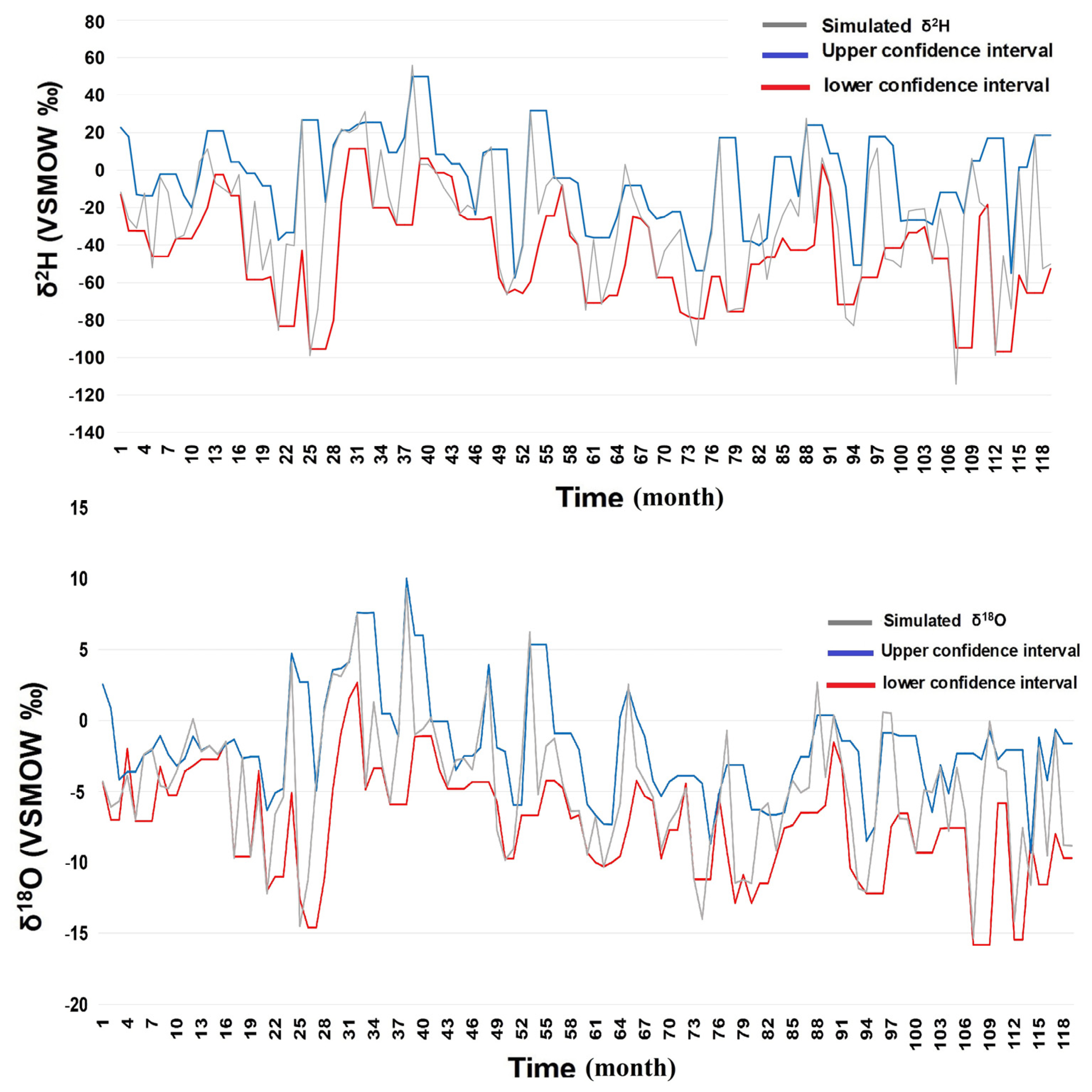
3.4. Evaluation Procedure and Uncertainty Analysis of the Developed Model

To determine the most accurate model among the studied ones, several indicators such as coefficient of determination (R2), root-mean-squared error (RMSE), Nash–Sutcliffe efficiency (NSE), Akaike information criterion (AIC), and Bayesian information criterion (BIC) were used to validate the accuracy of the developed models. R2, NSE, and RMSE can provide information about how well the model fits the data, while AIC and BIC can provide information about the relative quality of different models while taking into account their complexity. By considering multiple measures, the most accurate model can be identified. After determining the most accurate model according to the RMSE, R2, AIC, NSE, and BIC methods, bootstrap uncertainty analysis was applied to assess the robustness of its predictions. This allowed for the estimation of the uncertainty in the chosen model and provided a more comprehensive evaluation of its performance.

3.5. Wavelet Coherency Analyses of Studied Parameters

After identifying the dominant predictors that influence the stable isotope signatures of precipitation, BWC and PWC analyses were used to investigate the multi-scale associations between the stable isotope signatures of precipitation and the dominant predictors influencing it. Firstly, BWC analysis was conducted, considering the role of each dominant predictor on the stable isotope signatures of precipitation. BWC is a measure used to study the correlation between two variables at different frequencies or scales over time. This method can help to determine the relationship and patterns between two variables whose correlation might not be clear when observing them separately [48]. It is noteworthy to mention that interrelationships exist among the dominant predictors influencing the BWC analysis. To unveil these relationships between the predictors, the concurrent or partial role of various dominant predictors in the stable isotope signatures of precipitation was studied using PWC analysis [49,50]. The coherence analysis and relationships between the various parameters were quantified using average wavelet coherence (AWC) [48,51].
In this study, various packages in the R language [52] were used to develop models, perform validation studies using R2, RMSE, NSE, AIC, and BIC, conduct uncertainty analysis using bootstrap, and perform wavelet coherence analysis. Details of the specific packages used are provided at the end of this manuscript.

4. Results and Discussion

4.1. Selection of the Optimum Predictors

In this section, the selection of the optimum predictors for simulating stable isotope signatures in Tehran precipitation is described. Several parameters that may influence stable isotope signatures were analysed for potential correlation using Pearson correlation analysis and Spearman’s rank correlation at a 95% confidence level. The results showed that temperature and the amount of precipitation have notable influence on stable isotope (δ18O and δ2H) signatures in precipitation, while the role of other parameters, including teleconnection indices, is negligible (Figure 4). The precipitation amount shows a negative correlation with stable isotope signatures due to the precipitation amount effect, while temperature shows a positive correlation with stable isotope signatures. In moderate- and high-latitude stations like Tehran, an increase in temperature causes more intense evaporation, which results in raindrops accumulating heavier isotopes. A moderate correlation has been observed between different input parameters such as a negative correlation between temperature and precipitation as well as a positive correlation between vapor pressure and temperature. As temperature increases, the air can hold more water vapor, which means that the saturation vapor pressure also increases. Among teleconnection indices, only SOI and BEST show a strong negative correlation. To prevent multicollinearity, the teleconnection index BEST was removed from the list of predictors.

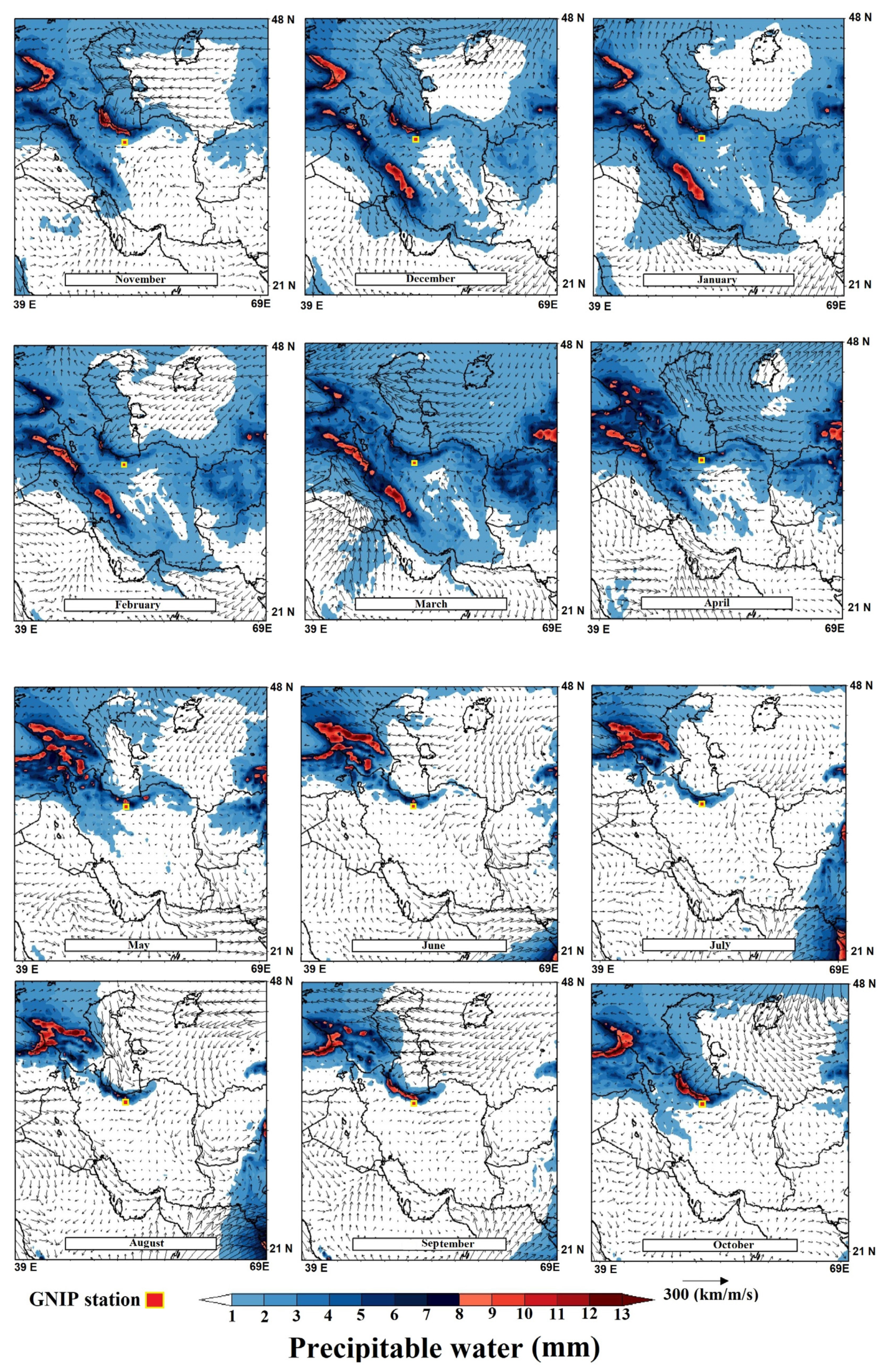
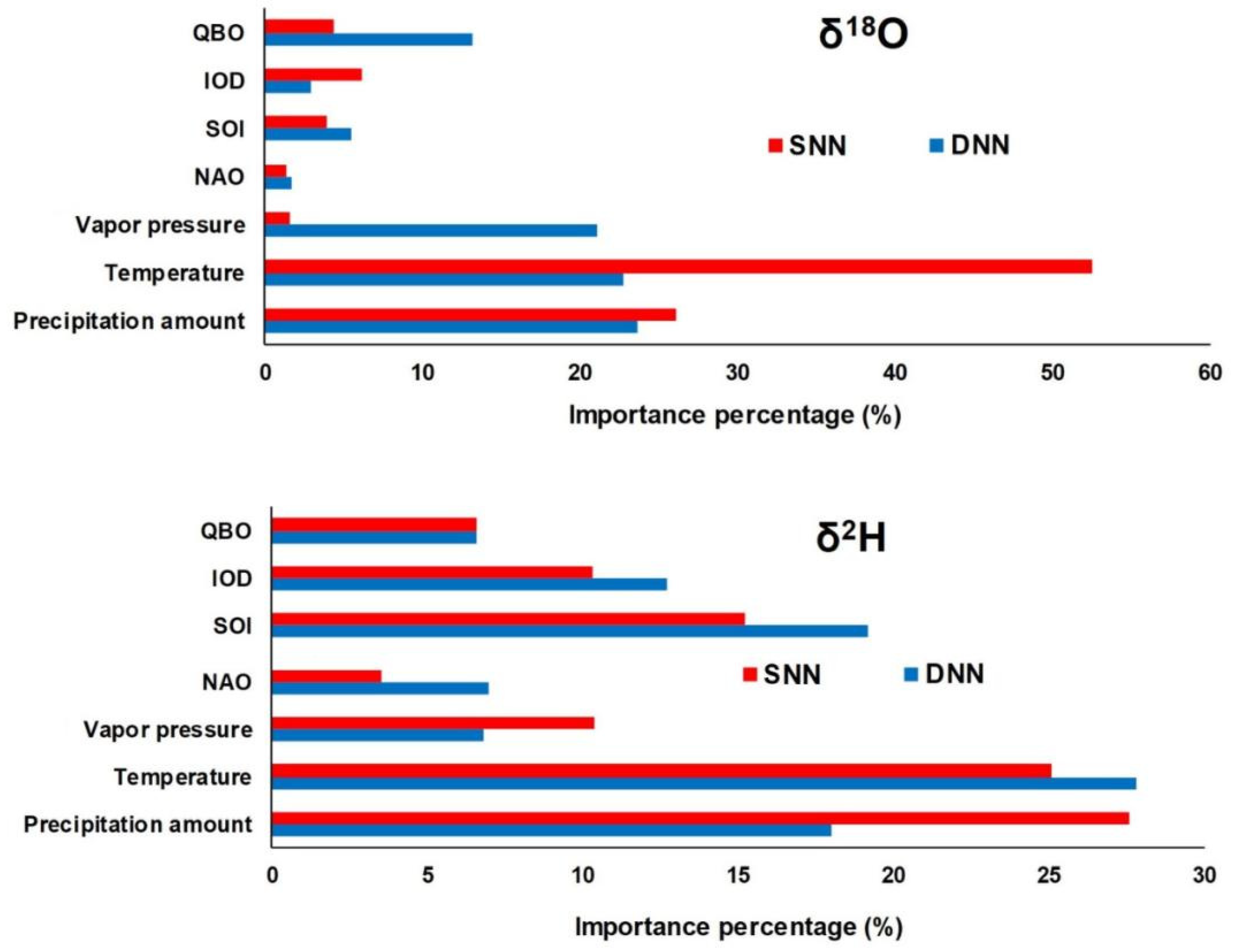
4.2. The Impacts of the Regional and the Local Components on the Stable Isotope Signatures of Precipitation in Tehran

The importance of the dominant local and regional components influencing precipitation in Tehran was determined using the ANNs’ models (Figure 5). The results of the SNN model demonstrated that the dominant factors affecting the stable isotope signatures of precipitation were air temperature and precipitation amount. However, regional parameters (teleconnection indices) played a minor role. On the other hand, the DNN model outputs depicts the dominant impacts of vapour pressure, air temperature, and precipitation amount on the stable isotope signatures of precipitation, whereas SOI, air temperature, and precipitation amount played dominant roles for δ2H signatures. The significant role of local parameters, such as the precipitation amount and air temperature that predominantly control the stable isotope signatures of precipitation, has been investigated in some studies [6,53,54,55,56,57]. However, the negligible role of teleconnection indices (regional parameters) that control stable isotope signatures of precipitation has been mentioned in other studies [21,22].

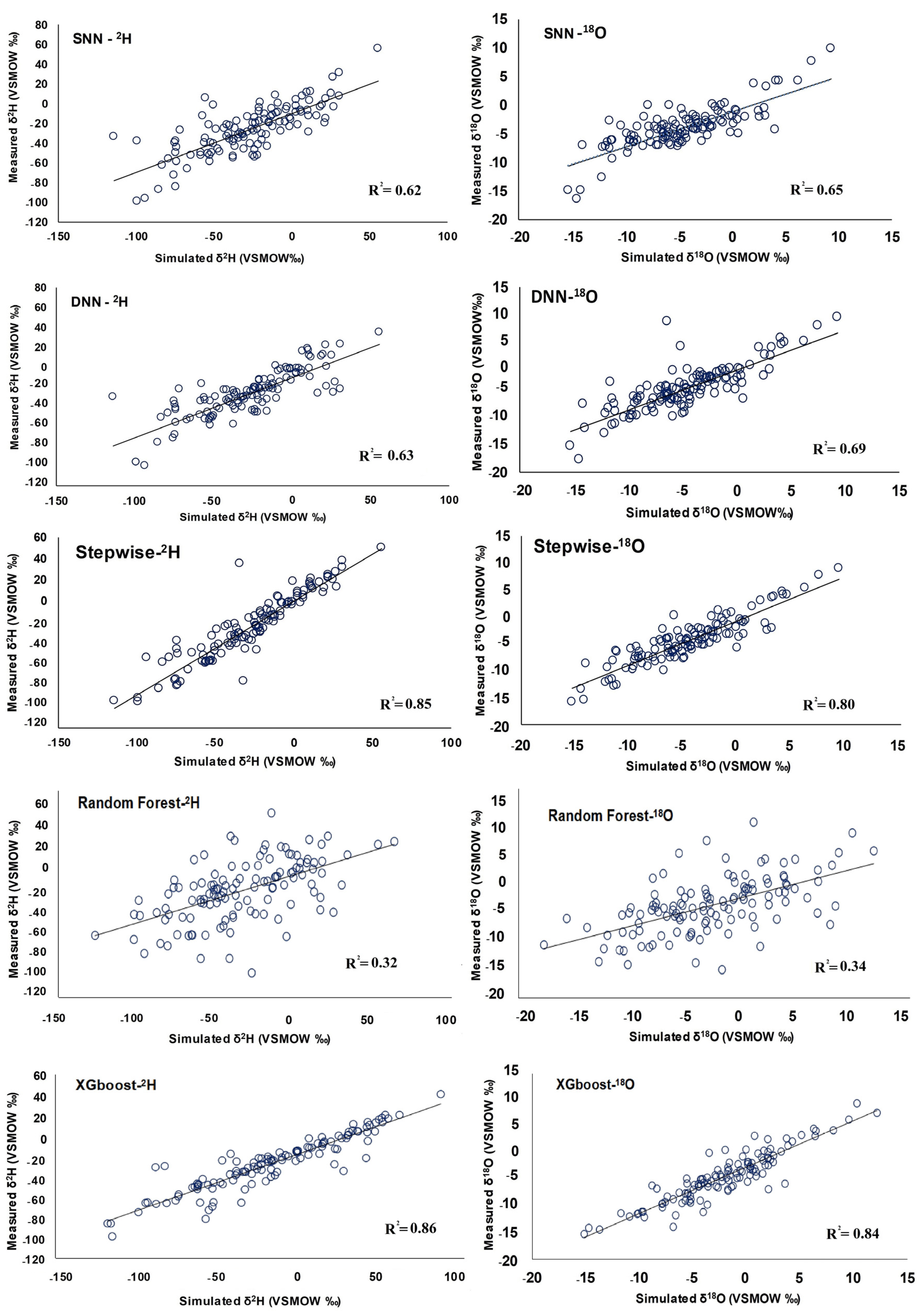
4.3. Simulation of the Stable Isotope Signatures in Precipitation by Various Machine Learning Models and Their Validation

The stable isotope signatures in Tehran precipitation were simulated using various machine learning models, including DNN, SNN, ensemble learning models such as XGBoost and RF, and stepwise regression methods. The results showed that the DNN and SNN models had low R2 values and high RMSE, NSE, AIC, and BIC values, indicating that they were not capable of accurately predicting stable isotope signatures. In contrast, models based on stepwise techniques were able to simulate stable isotope signatures with higher levels of accuracy. Among the ensemble learning models, XGBoost is the most accurate due to its highest R2 values and lowest RMSE, NSE, AIC, and BIC values, while the RF model had the lowest accuracy (Table 2). The low accuracy of some of the developed models may be due to overfitting, which can occur if the model is too complex and captures noise in the training data, or if the training set is too small.
Plotting real vs. simulated stable isotope signatures in precipitation shows good matching in both models developed by XGboost for δ18O and δ2H (Figure 6). Other models, such as ANNs and stepwise, also show good matching in their simulations. However, the simulation made by the RF model shows the lowest accuracy level and very low matching. The results obtained during this study are in agreement with previous studies that tried to simulate stable isotope signatures using machine learning techniques. For instance, the high accuracy of the XGboost model was also observed in the study of Nelson and his colleagues [35] in Europe. In the study of Erdelyi and colleagues [37], the RF model showed better accuracy compared to this study. In the study of Heydarizad and colleagues [13], the ANNs showed approximately the same accuracy as this study when simulating the stable isotope content of precipitation in Bangkok. The stepwise model was also been applied to simulate the stable isotope signatures of precipitation in some places such as the Middle East region [24] and showed high accuracy like the stepwise model in the current study. Since the stable isotope data in all these studies were mainly provided by GNIP, the slight difference observed in the accuracy of the developed model may have been due to differences that exist in the structure of the isotope datasets in these stations. Although the stable isotope signatures in precipitation predicted by the XGboost model have appropriate levels of precision, higher accuracy can also be achieved by improving the number of predictors involved in the models. Adding new predictors to the models, such as cloud microphysical parameters, cloud-top temperature (CTT), cloud-top pressure (CTP), atmospheric stability (ω), and outgoing long-wave radiation (OLR), can increase accuracy [21]. However, these parameters are not available for the entire stable isotope time series in Tehran from 1961–2005 and only cover small parts of the stable isotope dataset. Applying these parameters in models simulating stable isotope signatures of precipitation leads to a significant increase in model accuracy. In addition, focusing on hybrid algorithms, such as machine learning wavelet transform algorithms or hybrid reinforcement and deep learning algorithms, can also help to achieve more accurate models when simulating the stable isotope signatures of precipitation.
The level of uncertainty in the simulations of the XGboost model, which was the most accurate model in this study, was determined using the bootstrap technique. A 95% confidence interval was established for the simulated data, providing a better understanding of the range of estimates associated with the model. Figure 7 displays the lower and upper bounds of the 95% confidence interval for stable isotope signatures in precipitation in Tehran. The majority of the simulated stable isotope data for both δ18O and δ2H fell within the confidence intervals, indicating that the XGboost model accurately predicted the stable isotope values. However, during several short periods, the simulated stable isotope data exceeded the upper confidence interval bound, indicating that the model underestimated extremely the high values, or fell below the lower confidence interval bound, indicating that the model overestimated the extremely low values.

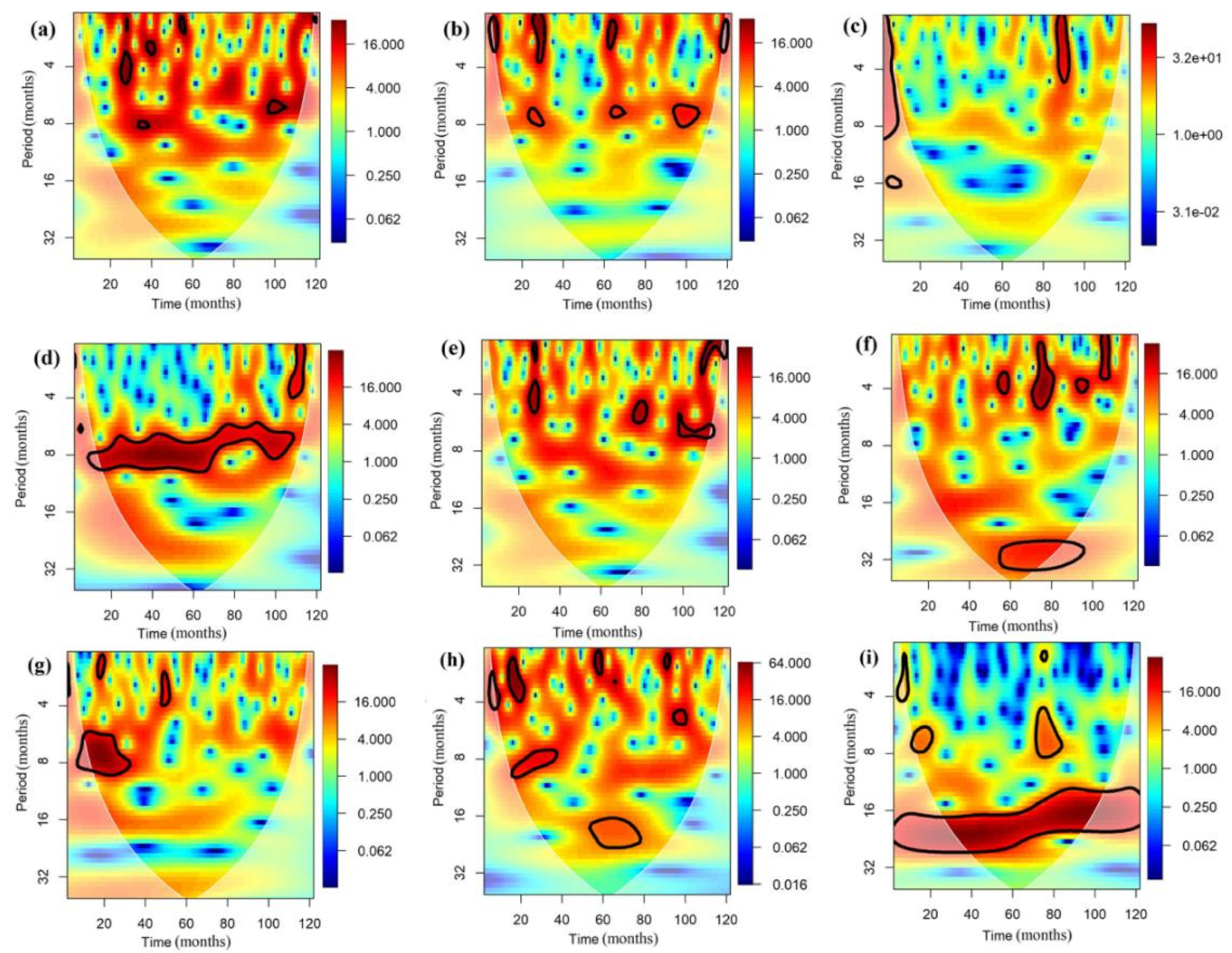
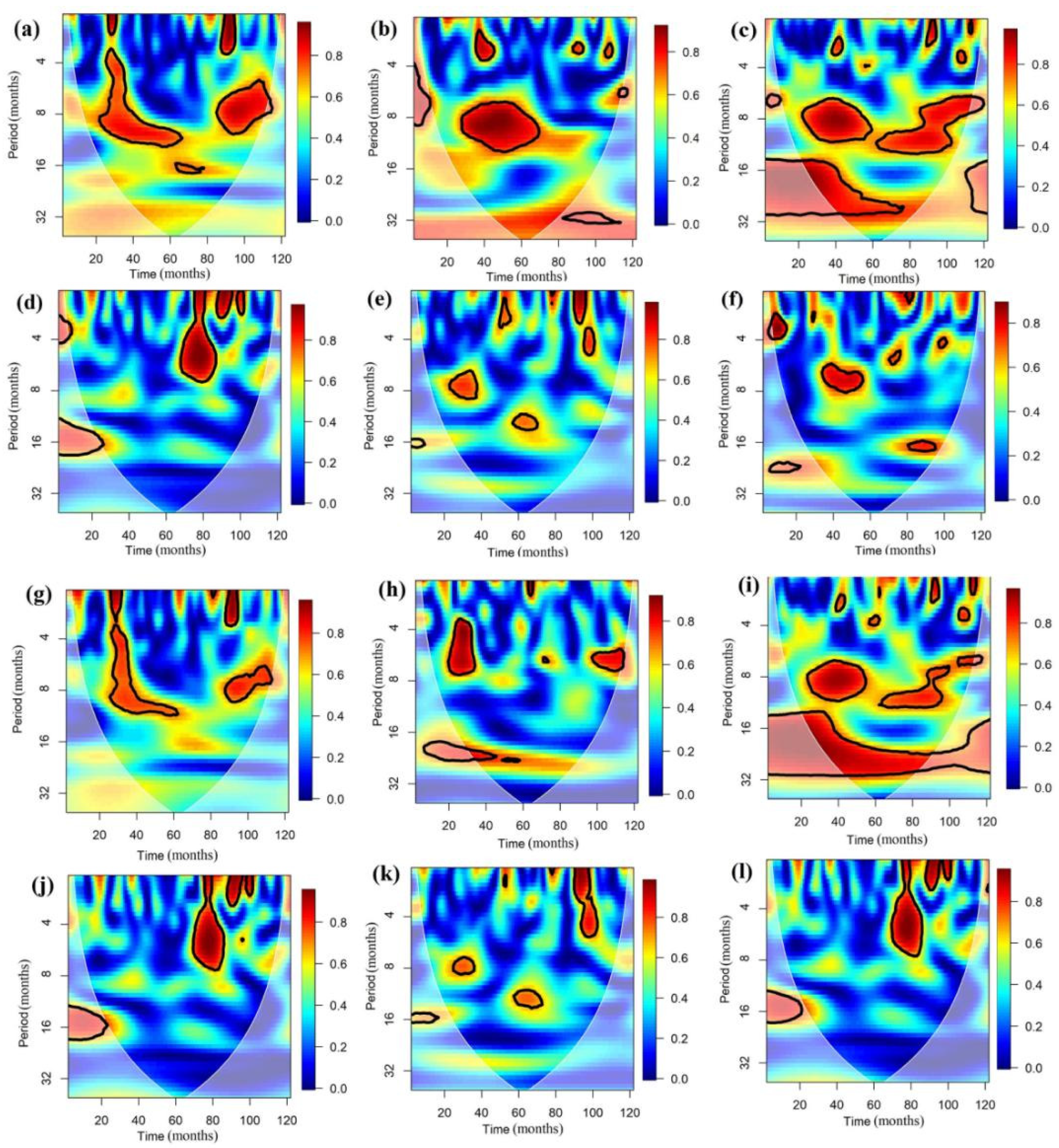
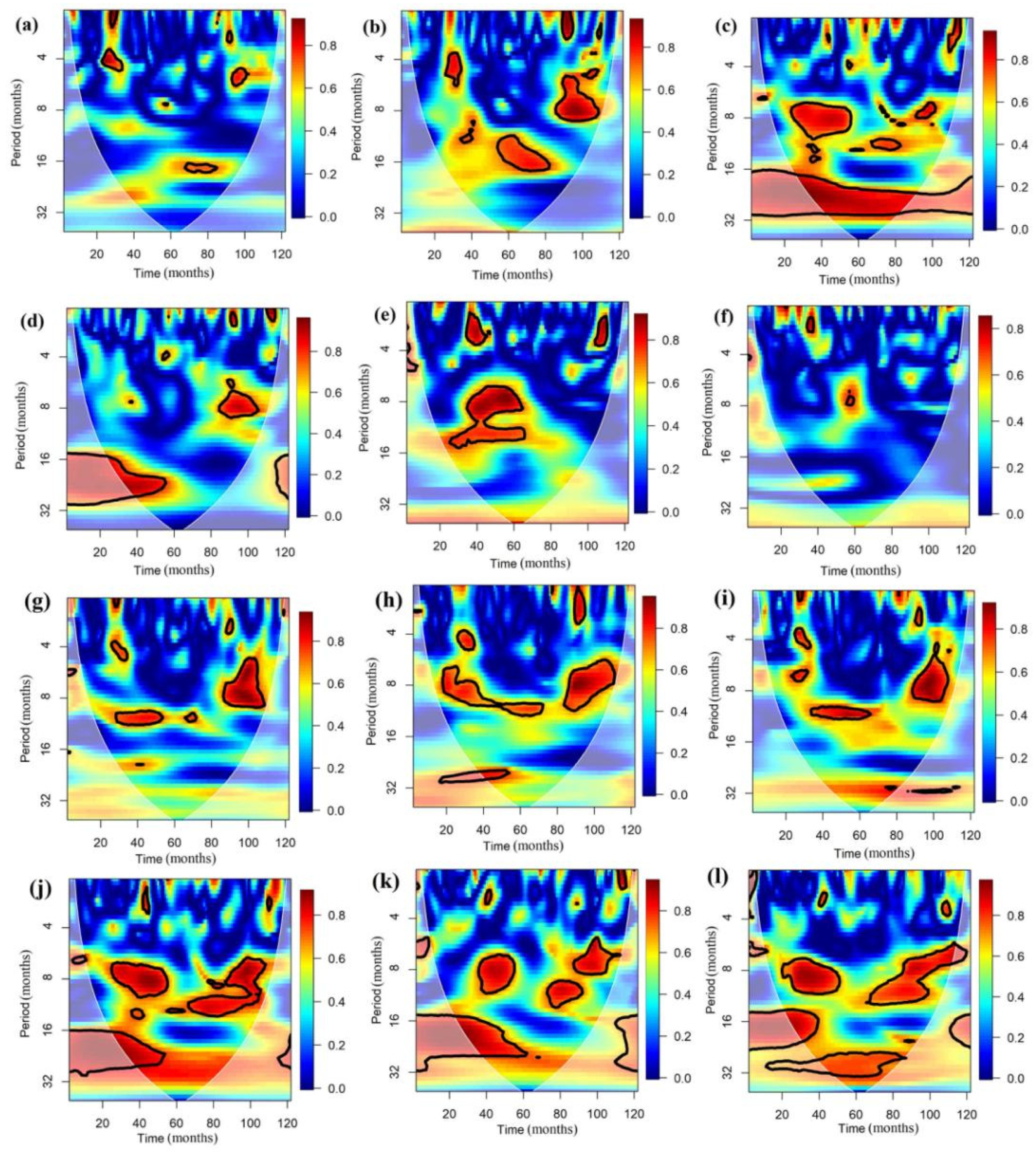
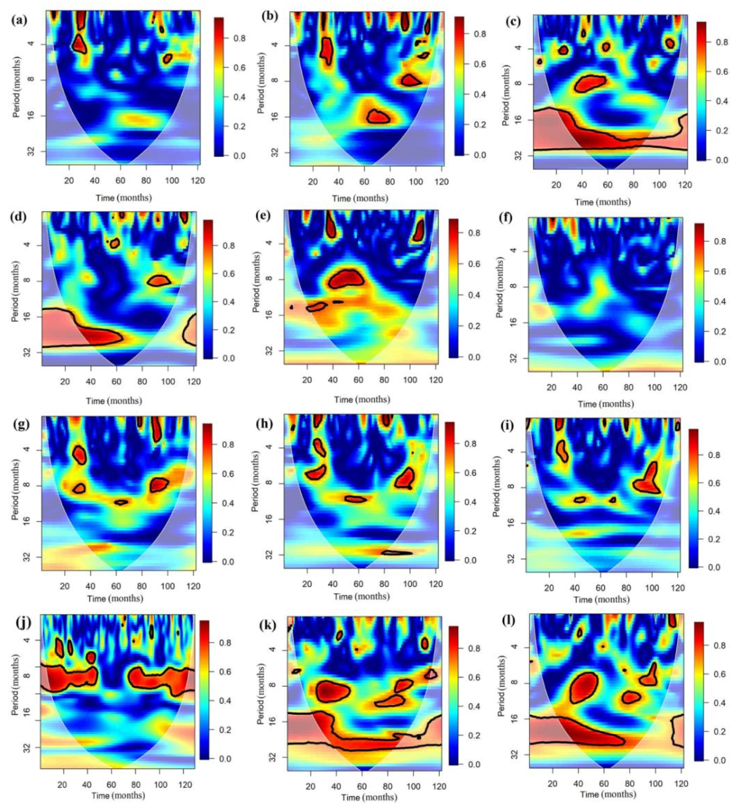
4.4. Studying the Multiscale Coherence Analysis of Stable Isotope Signatures and Climate Parameters in Tehran Precipitation

This section explores the relationship between stable isotope signatures and climate parameters in Tehran precipitation using multiscale coherence analysis. Continuous wavelet transform analysis (CWT) with the Morlet wavelet is applied to investigate the variations observed in the dominant predictors obtained by the ANNs models and stable isotope signatures. Figure 8 presents the CWT spectra of the dominant predictors and target variable, with black contour lines indicating statistically significant wavelet power at 5% significance levels.
The CWT analysis demonstrated a notable periodicity of 6–8 months, but only for the temperature and QBO indices time series. However, periodicity in other time series in this study was very localised in time, indicating the notable role played by local and temporary climatological conditions in the stable isotope signatures of precipitation. The wavelet coherence between the dominant predictors and the stable isotope signatures of precipitation was examined using BWC and PWC analyses.
The BWC analysis results are shown in Figure 9, where the BWC coherence relationship mainly ranges from 16 to 32 months for both δ18O–temperature and δ2H–temperature pairs. For δ18O–precipitation and δ2H–precipitation pairs, coherence relations are observed that range from 4 to 8 months, extending up to 16 months for the δ18O–precipitation pair. However, the coherence relation for δ18O–vapor pressure and δ2H–SOI pairs is intermittent and localised in the time domain. In addition to the dominant long 16–32-month scale and intra-annual scale of 4–8 months of coherence observed between the studied pairs, seasonal scale (less than 4 months) coherence has also been observed. However, these seasonal coherence relations are negligible and intermittent for the studied pairs. The coherence relation for δ18O–vapor pressure, as well as stable isotopes and teleconnection indices pairs such as δ18O–NAO, δ18O–IOD, δ18O–QBO, δ2H–NAO, δ2H–IOD, δ2H–SOI, and δ2H–QBO pairs, is highly intermittent and localised in the time domain.
To determine which dominant predictor has the strongest influence on the stable isotope signatures, the average wavelet coherence (AWC) was conducted. The AWC values obtained for BWC analysis for the studied datasets have been tabulated in Table 3. Studying the values of AWC shows that δ18O–temperature and δ2H–temperature pairs shows the highest AWC values.
In addition to BWC, PWC analysis was also conducted on the studied time series. This analysis is particularly useful in cases where the target value is influenced by multiple predictors as it can determine the partial correlation between the target parameter and each predictor while eliminating the influence of other predictors. Figure 10 and Figure 11 display the PWC spectrum for δ18O and δ2H stable isotopes. The highest AWC values were observed in the relationship between δ18O and temperature and δ2H and temperature, with a periodicity of 16–32 months. In all the studied cases, AWC values of PWC analysis demonstrated lower values compared to the corresponding BWC analysis (Table 3). This confirms the existence of an interrelationship of the dominant predictors in stable isotope signatures of precipitation. In general, predictors normally influence each other and the target variable.
According to BWC and PWC analysis, temperature is the dominant predictor influencing the stable isotope signatures of precipitation, while precipitation has a lower impact. The dominant role of temperature in stable isotope signatures of precipitation has also been confirmed by models developed by machine learning techniques. The dominant role of temperature on stable isotope signatures of precipitation in semi-arid and arid regions in middle and high latitudes has been mentioned in previous studies such as [3,4,23,38]. This is because the humidity in the atmosphere of these regions is low and temperature rises in a dominant manner, increasing the evaporation rate (secondary evaporation). This has a direct influence on raindrops and causes enrichment in the stable isotope signatures of precipitation.

5. Conclusions

In this study, it was found that local parameters, such as temperature and precipitation amounts, have a dominant influence on the stable isotope signatures in precipation around Tehran, while most regional parameters, such as teleconnection indices, play minor roles. It was also shown that the ensemble machine learning algorithm XGboost outperforms other machine learning models in simulating the stable isotope signatures in precipitation. These findings contribute to the understanding of the factors that influence stable isotope signatures in precipitation and demonstrate the potential of machine learning algorithms for simulating these signatures.
The results of this study have several implications for future research. First, they suggest that the focus of future studies could be turned to developing hybrid algorithms, such as machine learning wavelet transform algorithms or hybrid reinforcement and deep learning algorithms, to achieve more accurate models. Second, they indicate that the accuracy of the models could be improved by increasing the number of input parameters and considering microphysical parameters or satellite-derived parameters. Third, they suggest that changes to the structure of the model, such as using leave-one-out cross-validation (LOOCV) instead of simple v-fold or k-fold cross-validation, could also improve model performance.
In conclusion, valuable insights into the factors that influence stable isotope signatures in precipitation were provided by this study and the potential of machine learning algorithms for simulating these signatures was demonstrated. The results suggest several pathways via which future work can further improve the accuracy of these simulations.

Author Contributions

Conceptualisation, M.H. and L.G.; methodology, L.G.; software, M.H.; validation, L.G., M.H. and M.M.; formal analysis, M.H.; investigation, M.H.; resources, M.S.G.; writing—original draft preparation, M.H. and M.S.G.; writing—review and editing, M.S.G. and M.H.; and project administration, L.G. and M.H. All authors have read and agreed to the published version of the manuscript.

Funding

This research received no external funding.

Institutional Review Board Statement

Not applicable.

Informed Consent Statement

Not applicable.

Data Availability Statement

Data will be available upon request.

Acknowledgments

The first author acknowledges the postdoctoral fellowship (no. 202323310039) awarded by the School of Ocean and Earth Science at Tongji University, China. L.G. has received partial support obtained from the Xunta de Galicia under Project ED431C 2021/44 (Programa de Consolidación e Estructuración de Unidades de Investigación Competitivas (Grupos de Referencia Competitiva) and Consellería de Cultura, Educación e Universidade). The authors also thank the Global Network of Isotopes in Precipitation (GNIP) for providing the precipitation isotope data for the Tehran station. The authors thank the National Oceanic and Atmospheric Administration (NOAA) and the US Department of Commerce for providing the teleconnection index datasets used in this study.

Data Tools

The required R packages in this study were “neuralnet”, “keras”, “biwavelet”, “wavelets”, “readr”,”tidyverse”, “caret”, “leaps”, “MASS”, “olsrr”, “GGally”, “xgboost”, “stringr”, “e1071”, “data.table”, “mlr”, “ParamHelpers”, “rts”, “dplyr”, “ncdf4”, “lubridate”, “reshape2”, “rsample”, “corrplot”, “randomForest”, “devtools”, “tidyverse”, “biwavelet”, “boot”, “AICcmodavg”, “flexmix”, “mc2d”, “lhs”, “fitdistrplus”, “ie2misc”, “openxlsx”, and“Metrics”.

Conflicts of Interest

The authors declare no conflict of interest.

References

  1. Bagheri, R.; Bagheri, F.; Karami, G.H.; Jafari, H. Chemo-isotopes (18O & 2H) signatures and HYSPLIT model application: Clues to the atmospheric moisture and air mass origins. Atmos. Environ. 2019, 215, 116892. [Google Scholar] [CrossRef]
  2. Rezaei, A.; Zare, M.; Raeisi, E.; Ghanbari, R.N. Interaction of a Fresh Water Lake and a Karstic Spring via a Syncline Fold. Groundwater 2013, 51, 305–312. [Google Scholar] [CrossRef] [PubMed]
  3. Mohammadzadeh, H.; Heydarizad, M. A conceptual model for water resources circulation patterns in Andarokh-Kardeh region (NE, Iran). Geochemistry 2020, 80, 125593. [Google Scholar] [CrossRef]
  4. Heydarizad, M.; Minaei, F.; Mayvan, J.E.; Mofidi, A.; Minaei, M. Spatial distribution of stable isotopes ((18)O and (2)H) in precipitation and groundwater in Iran. Isotopes Environ. Health Stud. 2021, 57, 400–419. [Google Scholar] [CrossRef] [PubMed]
  5. Chitsazan, M.; Karimi Vardanjani, H.; Karimi, H.; Charchi, A. A comparison between karst development in two main zones of Iran: Case study—Keyno anticline (Zagros Range) and Shotori anticline (Central Iran). Arab. J. Geosci. 2015, 8, 10833–10844. [Google Scholar] [CrossRef]
  6. Kazemi, G.A.; Ichiyanagi, K.; Shimada, J. Isotopic characteristics, chemical composition and salinization of atmospheric precipitation in Shahrood, northeastern Iran. Environ. Earth Sci. 2015, 73, 361–374. [Google Scholar] [CrossRef]
  7. Moghadam, H.M.; Bagheri, R.; Karami, G.H.; Jafari, H. Groundwater Origin in Qanats, Chemo-Isotopic, and Hydrogeological Evidence. Groundwater 2020, 58, 771–776. [Google Scholar] [CrossRef]
  8. Tindall, J.C.; Valdes, P.J.; Sime, L.C. Stable water isotopes in HadCM3: Isotopic signature of El Niño–Southern Oscillation and the tropical amount effect. J. Geophys. Res. Atmos. 2009, 114, 111. [Google Scholar] [CrossRef] [Green Version]
  9. Martin, N.J.; Conroy, J.L.; Noone, K.M.; Cobb, B.L.; Konecky, S.R. Seasonal and ENSO Influences on the Stable Isotopic Composition of Galápagos Precipitation. J. Geophys. Res. Atmos. 2018, 123, 261–275. [Google Scholar] [CrossRef] [Green Version]
  10. Gao, J.; He, Y.; Masson-Delmotte, V.; Yao, T. ENSO Effects on Annual Variations of Summer Precipitation Stable Isotopes in Lhasa, Southern Tibetan Plateau. J. Clim. 2018, 31, 1173–1182. [Google Scholar] [CrossRef]
  11. Cai, Z.; Tian, L.; Bowen, G.J. ENSO variability reflected in precipitation oxygen isotopes across the Asian Summer Monsoon region. Earth Planet. Sci. Lett. 2017, 475, 25–33. [Google Scholar] [CrossRef]
  12. Ichiyanagi, K.; Yamanaka, M. Interannual variation of stable isotopes in precipitation at Bangkok in response to El Ñino Southern Oscillation. Hydrol. Process. 2005, 19, 3413–3423. [Google Scholar] [CrossRef]
  13. Heydarizad, M.; Pumijumnong, N. Predication of stable isotopes (18O and 2H) in precipitation of Bangkok metropolitan using artificial neural network. In Proceedings of the in Proceedings of the 5th International Electronic Conference on Atmospheric Sciences; MDPI: Basel, Switzerland, 2022. [Google Scholar]
  14. Tabari, H.; Aragi, H.; Hosseinzadeh Talaee, P. Impact of the North Atlantic Oscillation on streamflow in Western Iran. Hydrol. Process. 2014, 28, 4411–4418. [Google Scholar] [CrossRef]
  15. Sabziparvar, A.A.; Movahedi, S.; Asakereh, H.; Maryanaji, Z.; Masoodian, S.A. Geographical factors affecting variability of precipitation regime in Iran. Theor. Appl. Climatol. 2015, 120, 367–376. [Google Scholar] [CrossRef]
  16. Nazemosadat, M.J. ENSO’ s Impact on the Occurrence of Autumnal Drought in Iran. Drought Netw. News 1999, 11, 65. [Google Scholar]
  17. Pourasghar, F.; Tozuka, T.; Jahanbakhsh, S.; Sari Sarraf, B.; Ghaemi, H.; Yamagata, T. The interannual precipitation variability in the southern part of Iran as linked to large-scale climate modes. Clim. Dyn. 2012, 39, 2329–2341. [Google Scholar] [CrossRef]
  18. Heydarizad, M.; Raeisi, E.; Sori, R.; Gimeno, L.; Nieto, R.; Heydarizad, M.; Raeisi, E.; Sori, R.; Gimeno, L.; Nieto, R. The Role of Moisture Sources and Climatic Teleconnections in Northeastern and South-Central Iran’s Hydro-Climatology. Water 2018, 10, 1550. [Google Scholar] [CrossRef] [Green Version]
  19. Lachniet, M.S.; Patterson, W.P. Use of correlation and stepwise regression to evaluate physical controls on the stable isotope values of Panamanian rain and surface waters. J. Hydrol. 2006, 324, 115–140. [Google Scholar] [CrossRef]
  20. McNeese, B. Stepwise Regression. Available online: https://www.spcforexcel.com/knowledge/root-cause-analysis/stepwise-regression (accessed on 10 March 2023).
  21. Heydarizad, M.; Pumijumnong, N.; Minaei, M.; Mayvan, J.E.; Mansourian, D. A comprehensive study of the parameters affecting the stable isotopes in the precipitation of the Bangkok metropolitan area using model-based statistical approaches. Isotopes Environ. Health Stud. 2023, 59, 161–179. [Google Scholar] [CrossRef]
  22. Heydarizad, M. Meteoric Water Lines of Iran for Various Precipitation Sources; Shiraz University: Shiraz, Iran, 2018. [Google Scholar]
  23. Mohammadzadeh, H.; Mayvan, J.E.; Heydarizad, M. The effects of moisture sources and local parameters on the 18O and 2H contents of precipitation in the west of Iran and the east of Iraq. Tellus B Chem. Phys. Meteorol. 2020, 72, 1–15. [Google Scholar] [CrossRef] [Green Version]
  24. Heydarizad, M.; Gimeno, L.; Sorí, R.; Minaei, F.; Mayvan, J.E. The Stable Isotope Characteristics of Precipitation in the Middle East Highlighting the Link between the Köppen Climate Classifications and the δ18O and δ2H Values of Precipitation. Water 2021, 13, 2397. [Google Scholar] [CrossRef]
  25. Banerjee, P.; Singh, V.S.; Chatttopadhyay, K.; Chandra, P.C.; Singh, B. Artificial neural network model as a potential alternative for groundwater salinity forecasting. J. Hydrol. 2011, 398, 212–220. [Google Scholar] [CrossRef]
  26. Barzegar, R.; Asghari Moghadam, A. Combining the advantages of neural networks using the concept of committee machine in the groundwater salinity prediction. Model. Earth Syst. Environ. 2016, 2, 26. [Google Scholar] [CrossRef] [Green Version]
  27. Mcculloch, W.; Pitts, W. A Logical Calculus of Ideas Immanent in Nervous Activity. Bull. Math. Biophys. 1943, 5, 127–147. [Google Scholar] [CrossRef]
  28. Hu, C.; Wu, Q.; Li, H.; Jian, S.; Li, N.; Lou, Z. Deep Learning with a Long Short-Term Memory Networks Approach for Rainfall-Runoff Simulation. Water 2018, 10, 1543. [Google Scholar] [CrossRef] [Green Version]
  29. Sahour, H.; Gholami, V.; Vazifedan, M. A comparative analysis of statistical and machine learning techniques for mapping the spatial distribution of groundwater salinity in a coastal aquifer. J. Hydrol. 2020, 591, 125321. [Google Scholar] [CrossRef]
  30. Chien, J.-T. Chapter 7—Deep Neural Network. In Source Separation and Machine Learning; Chien, J.-T., Ed.; Academic Press: Cambridge, MA, USA, 2019; pp. 259–320. ISBN 978-0-12-817796-9. [Google Scholar]
  31. Heydarizad, M.; Pumijumnong, N.; Gimeno, L. A Comparative Analysis of Analytical Hierarchy Process and Machine Learning Techniques to Determine the Fractional Importance of Various Moisture Sources for Iran’s Precipitation. Environ. Sci. Proc. 2022, 19, 29. [Google Scholar] [CrossRef]
  32. Dehghani, M.; Saghafian, B.; Nasiri Saleh, F.; Farokhnia, A.; Noori, R. Uncertainty analysis of streamflow drought forecast using artificial neural networks and Monte-Carlo simulation. Int. J. Climatol. 2014, 34, 1169–1180. [Google Scholar] [CrossRef]
  33. Hamidi, O.; Poorolajal, J.; Sadeghifar, M.; Abbasi, H.; Maryanaji, Z.; Faridi, H.; Tapak, L. A comparative study of support vector machines and artificial neural networks for predicting precipitation in Iran. Theor Appl Clim. 2014, 119, 723–731. [Google Scholar] [CrossRef]
  34. Aggarwal, P. ML | XGBoost (eXtreme Gradient Boosting). Available online: https://www.geeksforgeeks.org/ml-xgboost-extreme-gradient-boosting/ (accessed on 11 October 2022).
  35. Nelson, D.B.; Basler, D.; Kahmen, A. Precipitation isotope time series predictions from machine learning applied in Europe. Proc. Natl. Acad. Sci. USA 2021, 118, e2024107118. [Google Scholar] [CrossRef]
  36. Erdélyi, D.; Hatvani, I.G.; Jeon, H.; Jones, M.; Tyler, J.; Kern, Z. Predicting spatial distribution of stable isotopes in precipitation by classical geostatistical- and machine learning methods. J. Hydrol. 2023, 617, 129129. [Google Scholar] [CrossRef]
  37. Erdélyi, D.; Kern, Z.; Nyitrai, T.; Hatvani, I. Predicting the spatial distribution of stable isotopes in precipitation using a machine learning approach: A comparative assessment of random forest variants. GEM—Int. J. Geomath. 2023, 14, 14. [Google Scholar] [CrossRef]
  38. Clark, I.D.; Fritz, P. Environmental Isotopes in Hydrogeology; CRC Press/Lewis Publishers: Boca Raton, FL, USA, 1997; ISBN 1566702496. [Google Scholar]
  39. IAEA; GNIP. Global Network of Isotopes in Precipitation (GNIP); IAEA: Vienna, Austria, 2008. [Google Scholar]
  40. IAEA; GNIP. Precipitation Sampling Guide; IAEA: Vienna, Austria, 2014. [Google Scholar]
  41. NOAA. Available online: https://www.esrl.noaa.gov (accessed on 15 March 2023).
  42. Blazek, P.J.; Lin, M.M. Explainable neural networks that simulate reasoning. Nat. Comput. Sci. 2021, 1, 607–618. [Google Scholar] [CrossRef]
  43. Donges, N. Random Forest: A Complete Guide for Machine Learning. Available online: https://builtin.com/data-science/random-forest-algorithm (accessed on 14 March 2023).
  44. Zach, B. A Simple Introduction to Random Forests. Available online: https://www.statology.org/random-forests/ (accessed on 15 June 2023).
  45. Gradient Boosting with Intel® Optmization for XGBoost. Available online: https://www.intel.com/content/www/us/en/developer/articles/technical/gradient-boosting-with-xgboost.html (accessed on 17 June 2023).
  46. Frick, H.; Mahoney, M.; Silge, J.; Wickham, H. V-Fold Cross-Validation. Available online: https://rsample.tidymodels.org/reference/vfold_cv.html (accessed on 14 June 2023).
  47. Molinaro, A.M.; Simon, R.; Pfeiffer, R.M. Prediction error estimation: A comparison of resampling methods. Bioinformatics 2005, 21, 3301–3307. [Google Scholar] [CrossRef] [PubMed] [Green Version]
  48. Sreedevi, V.; Adarsh, S.; Nourani, V. Multiscale coherence analysis of reference evapotranspiration of north-western Iran using wavelet transform. J. Water Clim. Chang. 2021, 13, 505–521. [Google Scholar] [CrossRef]
  49. Ng, E.K.W.; Chan, J.C.L. Geophysical Applications of Partial Wavelet Coherence and Multiple Wavelet Coherence. J. Atmos. Ocean. Technol. 2012, 29, 1845–1853. [Google Scholar] [CrossRef]
  50. Hu, W.; Si, B. Technical Note: Improved partial wavelet coherency for understanding scale-specific and localized bivariate relationships in geosciences. Hydrol. Earth Syst. Sci. 2021, 25, 321–331. [Google Scholar] [CrossRef]
  51. Nalley, D.; Adamowski, J.; Biswas, A.; Gharabaghi, B.; Hu, W. A multiscale and multivariate analysis of precipitation and streamflow variability in relation to ENSO, NAO and PDO. J. Hydrol. 2019, 574, 288–307. [Google Scholar] [CrossRef]
  52. R core team. R: A Language and Environment for Statistical Computing; R core team: Vienna, Austria, 2018. [Google Scholar]
  53. Jeelani, G.; Bhat, N.A.; Shivanna, K. Use of δ18O tracer to identify stream and spring origins of a mountainous catchment: A case study from Liddar watershed, Western Himalaya, India. J. Hydrol. 2010, 393, 257–264. [Google Scholar] [CrossRef]
  54. Yang, Q.; Mu, H.; Guo, J.; Bao, X.; Martín, J.D. Temperature and rainfall amount effects on hydrogen and oxygen stable isotope in precipitation. Quat. Int. 2019, 519, 25–31. [Google Scholar] [CrossRef]
  55. Huang, L.; Wen, X. Temporal variations of atmospheric water vapor δD and δ18O above an arid artificial oasis cropland in the Heihe River Basin. J. Geophys. Res. Atmos. 2014, 119, 11–456. [Google Scholar] [CrossRef]
  56. Lone, S.A.; Jeelani, G.; Deshpande, R.D.; Mukherjee, A. Stable isotope (δ18O and δD) dynamics of precipitation in a high altitude Himalayan cold desert and its surroundings in Indus river basin, Ladakh. Atmos. Res. 2019, 221, 46–57. [Google Scholar] [CrossRef]
  57. Kohn, M.J.; Welker, J.M. On the temperature correlation of δ18O in modern precipitation. Earth Planet. Sci. Lett. 2005, 231, 87–96. [Google Scholar] [CrossRef]
Figure 1. (a) The location of Tehran in Iran and the location of the GNIP station in Tehran metropolitan area. (b) The main water bodies near Iran and the dominant air masses that influence the country.
Water 15 02357 g001
Figure 2. Monthly vapor pressure, precipitation amount, air temperature, and stable isotope signatures at the Tehran GNIP station for two periods: 1961–1987 and 2000–2004. Data obtained from the Global Network of Isotopes in Precipitation (GNIP) database.
Water 15 02357 g002
Figure 3. The monthly variations of wind speed, wind direction, and precipitable water over Iran.
Water 15 02357 g003
Figure 4. (a) Pearson correlation coefficients and (b) Spearman’s rank correlation for the studied parameters affecting the stable isotope content of precipitation in the Tehran GNIP station (* shows the pairs with statistical significance).
Water 15 02357 g004
Figure 5. The importance of the main local and regional parameters which controls the stable isotope signature of precipitation (Tehran GNIP station).
Water 15 02357 g005
Figure 6. Comparison between measured and simulated stable isotope signatures in Tehran GNIP station using R2 values.
Water 15 02357 g006
Figure 7. Confidence intervals using a bootstrap analysis for the simulated stable isotope content (δ18O and δ 2H) obtained from the XGboost model.
Water 15 02357 g007
Figure 8. Time-frequency spectra of the main predictors and stable isotope (δ18O and δ2H) signatures: (a) δ18O, (b) precipitation amount, (c) vapor pressure, (d) temperature, (e) δ2H, (f) SOI, (g) NAO, (h) IOD, and (i) QBO.
Water 15 02357 g008
Figure 9. BWC analysis of the main predictors and the stable isotope (δ18O and δ2H) signatures. The upper panels demonstrate the BWC analysis of δ18O with (a) precipitation amount, (b) vapor pressure, (c) temperature, (d) IOD, (e) NAO, and (f) QBO, while the lower panels show the BWC analysis of δ2H with (g) precipitation amount, (h) SOI, (i) temperature, (j) IOD, (k) NAO, and (l) QBO.
Water 15 02357 g009
Figure 10. PWC analysis between δ18O signatures in Tehran metropolitan precipitation and the main predictor variables: (a) δ18O vs. precipitation amount (excluding temperature), (b) δ18O vs. precipitation amount (excluding vapor pressure), (c) δ18O vs. temperature (excluding precipitation amount), (d) δ18O vs. temperature (excluding vapor pressure), (e) δ18O vs. vapor pressure (excluding Precipitation amount), and (f) δ18O vs. vapor pressure (excluding temperature), (g) δ18O vs. NAO (excluding precipitation amount), (h) δ18O vs. IOD (excluding precipitation amount), (i) δ18O vs. QBO (excluding precipitation amount), (j) δ18O vs. NAO (excluding temperature), (k) δ18O vs. IOD (excluding temperature), and (l) δ18O vs. QBO (excluding temperature).
Water 15 02357 g010
Figure 11. PWC analysis between δ2H signatures in Tehran metropolitan precipitation and the main predictor variables: (a) δ2H vs. precipitation amount (excluding temperature), (b) δ2H vs. precipitation amount (excluding vapor pressure), (c) δ2H vs. temperature (excluding precipitation amount), (d) δ2H vs. temperature (excluding vapor pressure), (e) δ2H vs. vapor pressure (excluding precipitation amount), (f) δ2H vs. vfapor pressure (excluding temperature), (g) δ2H vs. NAO (excluding precipitation amount), (h) δ2H vs. IOD (excluding precipitation amount), (i) δ2H vs. QBO (excluding precipitation amount), (j) δ2H vs. NAO (excluding temperature), (k) δ2H vs. IOD (excluding temperature), and (l) δ2H vs. QBO (excluding temperature).
Water 15 02357 g011
Table 1. Statistical characteristics of parameters in the analysis of Tehran precipitation.
ParameterMinMaxMeanStd. DeviationVariance
StatisticStatisticStatisticStd. errorStatisticStatistic
δ18O (VSMOW‰)−15.349.30−4.59±0.434.7222.28
δ2H (VSMOW‰)−114.2055.80−26.77±2.9332.281.04
Precipitation (mm)1.00117.0023.71±2.0622.69514.80
Temperature (°C)−4.1030.7013.03±0.748.2367.82
Vapor pressure (Pa)1.1028.706.47±0.283.059.32
NAO−2.472.16−0.23±0.0890.970.95
BEST−2.461.630.06±0.680.750.56
SOI−2.012.85−0.07±0.0820.900.82
IOD−0.050.940.12±0.0240.260.07
QBO−24.1814.16−2.28±0.9810.75115.50
Table 2. Evaluation of simulated δ18O and δ2H signatures in Tehran precipitation using the various evaluation metrics (AIC, BIC, R2, RMSE, and NSE).
IsotopeMethodXGboostDNNSNNRandom ForestStepwise
δ18O (VSMOW‰)AIC517.44605.20614.04680.12531.42
BIC531.42618.99628.02694.09545.10
R20.840.690.650.340.80
VNS0.830.680.640.330.80
RMSE1.972.832.933.852.08
δ2H (VSMOW‰)AIC965.571062.391083.061148.70972.14
BIC979.551076.371097.041162.75986.12
R20.860.630.620.320.85
VNS0.850.620.620.310.84
RMSE12.5418.7220.3926.7512.89
Table 3. The values of AWC calculated for BWC and PWC analysis between the stable isotope (δ18O and δ2H) signatures in precipitation and the main predictor variables. (P stands for precipitation amount, T stands for temperature, and V stands for vapor pressure).
CombinationAWCCombinationAWC
PWC18O2HBWC18O2H
Temperature
18O-T-P/2H-T-P0.450.4518O-T0.63
18O-T-V/2H-T-V0.430.422H-T 0.55
Precipitation
18O-P-T/2H-P-T0.350.318O-P0.62
18O-P-V/2H-P-V0.440.372H-P 0.50
Vapor pressure
18O-V-P0.44 18O-V0.53
18O-V-T0.32
SOI teleconnection
18O-NAO-P0.35 18O-NAO 0.33
18O-NAO-T0.44
18O-SOI-P0.33 18O-SOI 0.30
18O-SOI-T0.31
18O-IOD-P0.37 18O-IOD 0.31
18O-IOD-T0.44
18O-QBO-P0.38 18O-QBO 0.32
18O-QBO-T0.46
2H-NAO-P 0.302H-NAO 0.33
2H-NAO-T 0.32
2H-SOI-P 0.422H-SOI 0.42
2H-SOI-T 0.31
2H-IOD-P 0.312H-IOD 0.31
2H-IOD-T 0.32
2H-QBO-P 0.322H-QBO 0.33
2H-QBO-T 0.42
Disclaimer/Publisher’s Note: The statements, opinions and data contained in all publications are solely those of the individual author(s) and contributor(s) and not of MDPI and/or the editor(s). MDPI and/or the editor(s) disclaim responsibility for any injury to people or property resulting from any ideas, methods, instructions or products referred to in the content.

