1. Introduction
The estimation of streamflow plays a pivotal role in water resource management. It facilitates the forecasting of forthcoming flood events and contributes to the optimization of water demand processes, thereby serving as an indispensable component of effective and sustainable water system management [
1,
2,
3,
4]. The ability to forecast streamflow accurately can assist water resource managers in making informed decisions regarding the release of water from reservoirs, irrigation, and other water uses [
5,
6,
7]. The effectiveness of streamflow forecasting in water management has been demonstrated through the use of hydrological models to optimize the operation of reservoir systems to meet the demands of irrigation and hydropower generation [
8]. Streamflow forecasts are also utilized to issue flood warnings and aid emergency managers in preparing for, and responding to, flooding events. Furthermore, the accuracy and quality of hydrological forecasts play a vital role improving the efficiency of hydropower generation by allowing power companies to better align their generation schedules with available water resources [
9,
10].
Simulating streamflow is complex due to the intricate nature of the hydrologic system [
11]. A number of factors, encompassing precipitation, evaporation, groundwater recharge, and land use, changes impact streamflow estimation. The scarcity of precise and reliable data further exacerbates the difficulty in accurately estimating streamflow [
12]. Additionally, quantifying and modeling these factors is a challenging task [
13,
14]. Moreover, it is often challenging to obtain long-term streamflow data for model calibration, particularly in ungauged or inadequately gauged catchments. Therefore, developing accurate prediction models, particularly for ungauged catchments, is a daunting task. Furthermore, estimating streamflow entails increased uncertainty due to the combined impacts of land use development and climate change [
15,
16,
17].
The estimation of streamflow is further complicated by the nonlinearity and nonstationary of the hydrological system. Due to its nonlinearity, even small variations in input can lead to substantial changes in output. Previous studies have demonstrated how alterations in precipitation can have significant impacts on streamflow estimation [
18,
19,
20,
21]. Moreover, the hydrological modeling process uncertainty raises concerns from the simplified or incorrect representation of the hydrological system. Therefore, the lack of a full comprehension of the underlying mechanisms that govern streamflow exacerbates the challenge of creating accurate forecasting models [
3,
22]. A variety of modeling approaches are used to issue these forecasts, including empirical models and process-oriented models. Process-oriented models use mathematical equations to simulate the physical processes operating in the watershed and estimated streamflow. Several types of process-oriented hydrological models, such as conceptual models and physically based models, which rely on a high degree of spatial discretization, are employed for operational streamflow forecasting [
22].
The estimation of streamflow can be issued using hydrological models at various scales, including watersheds, regions, and even the continental scale. Several hydrological models have been developed to estimate streamflow on large scales, including the continental and global scale. Some notable examples of large-scale hydrological models include the Variable Infiltration Capacity (VIC) model [
23], the Land Dynamics (LaD) Model [
24], and, more recently, the GEOGloWS ECMWF Streamflow service [
25]. The models have been employed to simulate streamflow, furnishing valuable insights for water resource managers, thereby enabling them to make well-informed decisions.
In the Unites States, the National Weather Service (NWS) Advanced Hydrologic Prediction Service (AHPS) supplies streamflow forecasts and warnings for more than 3600 locations across the country [
26,
27]. However, those forecasts are specific to NWS River Forecast Centers (RFC). The system leverages streamflow forecasts, precipitation observations, and river-gauge measurements to issue flood and flash flood warnings. These alerts are communicated to the public through various channels, encompassing the NWS website, social media platforms, and emergency management agencies. Nonetheless, the National Research Council identified a discrepancy between the state-of-the-art modeling capabilities currently considered cutting edge and those utilized in the AHPS [
27]. This observation underscores the necessity to integrate more advanced hydrologic models. In 2016, the National Water Model (NWM), a group of physics-based, hydrodynamic, and hydrologic models, was implemented by NOAA’s Office of Water Prediction (OWP). The NWM is based on the Weather Research and Forecasting Model Hydrological modeling system (WRF–Hydro) framework [
28] and generates streamflow forecasts for over 2.7-million locations across the CONUS [
29].
Streamflow estimation is a key component of flood-risk mitigation. Thus, it is imperative to evaluate hydrological models’ performance. It is essential to compare the model’s predictions to observed data to validate the model and determine its capacity to reproduce in-land processes. Moreover, assessing the performance of hydrological models can help identify areas for improvement, including addressing model biases, improving the representation of key processes, and incorporating new data and observational capabilities. Additionally, continental-scale models are commonly used to support water management decisions and facilitate decision-making [
30]. Thus, evaluating the performance of continental scale models can assist in communicating the model’s capabilities and limitations to stakeholders, which can build trust in the model and its predictions.
The evaluation of continental-scale hydrological models is critical in ensuring their accuracy and reliability for various applications, such as water-resource management and flood forecasting. A key component of model evaluation involves comparing model estimates to observed data and assessing the model’s ability to reproduce historical streamflow patterns. Retrospective simulations are a valuable tool in assessing the performance of continental-scale hydrological models. This approach involves running the model using historical data and comparing its output with observed data from the same period. The retrospective analysis serves to evaluate the model’s ability to accurately simulate past hydrological conditions, identify sources of bias or error, and improve its performance. This analysis enables the identification of areas for model improvement, thereby increasing confidence in its predictions. Thus, the evaluation of retrospective simulations plays a crucial role in the continual improvement and refinement of continental-scale hydrological models.
This study aims to evaluate the performance of the NWM V2.1 through the analysis of the results of multi-decadal retrospective simulations across the contiguous United States (CONUS). The study identifies the limitations of the NWM as reported by the retrospective runs, which could be indicative of the necessary areas of improvement to enhance the operational runs. The study investigates the spatial and temporal variability of streamflow bias, with the objective of identifying instances and locations where the model underestimates or overestimates streamflow. Understanding the factors underlying the variations in the model’s performance is essential in this regard. Eventually, recommendations could be made to enhance the modeling of hydrologic processes across the US based on the determined biases.
3. Results
The accuracy of the NWM streamflow simulation was assessed by comparing with in-situ data using five evaluation statistics, namely KGE, PB, RMSE, NRMSE, and CC. The hourly streamflow data acquired from in-situ and retrospective simulations from February 1979 to December 2020 were used to analyze the Spatiotemporal Variability of the model accuracy. The basin drainage area and RFCs differences were considered.
3.1. Spatial Analysis
The findings derived from the evaluation metrics assessing the NWM streamflow simulations’ performance are illustrated in
Figure 2. The acquired results demonstrate that 57% of natural flow forecast points exhibit KGE values exceeding 0.5 (
Figure 2a), while 43% of forecast points associated with regulated flow present KGE values surpassing 0.5 (
Figure 2b). The outcomes reveal suboptimal model performance for forecast points situated within the MBRFC, ABRFC, and WGRFC. Conversely, the model exhibits a commendable performance in estimating streamflow within the NERFC, MARFC, and NWRFC. It is crucial to note that KGE values represent an overall estimation of the concordance between observed and simulated streamflow. In essence, KGE values may be influenced by errors related to correlation, variability, bias, or a combination of these metric components.
The variation in bias error across the different River Forecast Centers (RFCs) was investigated utilizing the percent bias (PB) metric. For natural flow, a satisfactory agreement between observed and simulated streamflow was achieved for 50% of the forecast points, with PB values ranging between −10% and 10%. PB values did not exhibit a discernible spatial distribution of bias error. However, a tendency for the model to underestimate streamflow values was observed in the eastern and northwestern portions of the contiguous United States, specifically within the NERFC, MARFC, SERFC, and NWRFC. Conversely, the model exhibited a propensity to overestimate streamflow in the central and western regions of the CONUS, predominantly over the MBRFC, ABRFC, and WGRFC (
Figure 2c).
The findings are also applicable to regulated flow forecast points, where the model tends to underestimate streamflow values in eastern RFCs and overestimate streamflow in central and western RFCs. The results revealed that 36% of regulated flow estimates demonstrated low bias error with PB values between −10% and 10%. Low PB values (close to zero) were primarily observed in the NERFC, MARFC, SERFC, NCRFC, and NWRFC (
Figure 2d). It is vital to note that RFCs where the NWM displays low PB values are characterized by high annual precipitation rates (reference). In contrast, high PB values were observed in regions with low annual precipitation rates. The results suggest that the NWM configuration is well-suited for regions dominated by high precipitation. In other words, the model structure and calibration parameters accurately represent surface runoff processes.
Natural streamflow estimates exhibited low RMSE values in the eastern and western RFCs of the CONUS, irrespective of drainage basin area (
Figure 2e). High RMSE values were observed for natural streamflow estimates in the central and eastern regions of the United States. In terms of drainage area, the highest RMSE values were associated with drainage basins encompassing an area exceeding 3000 km². Both RMSE and normalized NRMSE demonstrated optimal results for NWM streamflow estimates in the eastern and western RFCs. The NWM natural streamflow data displayed elevated NRMSE results in the central region, particularly in the MBRFC and portions of the CBRFC. Regulated flow data exhibited inferior performance compared to natural flow, as indicated by higher RMSE and NRMSE values (
Figure 2g,h) across the various RFCs within the CONUS. Regulated streamflow estimates yielded the most favorable outcomes in terms of RMSE and NRMSE values in the northeastern region, primarily for forecast points with a drainage area of less than 1000 km². NRMSE values below 5% were obtained for 86% of natural forecast points and 63% of regulated forecast points, respectively.
Overall, the model error outcomes in terms of RMSE and NRMSE indicate enhanced performance of the NWM in estimating natural streamflow. The obtained results can be attributed to the fact that regulated flow watersheds exhibit altered hydrological regimes due to the presence of water control structures, such as dams, weirs, and other hydraulic structures. These structures can significantly alter the timing and magnitude of downstream discharge. Consequently, it is challenging to capture the effects of these alterations on a continental-scale hydrological system. In essence, the NWM configuration may not be capable of simulating the intricate interactions between hydraulic structures and the hydrological system. Furthermore, regulated flow basins are often subject to human interventions, which can further complicate the hydrological regime, rendering it challenging for the NWM to accurately simulate streamflow.
Natural streamflow estimates demonstrated optimal results in terms of CC values (CC > 0.50) within the eastern and western RFC. The natural streamflow estimates exhibited the weakest correlation with in situ streamflow observations in the central region, particularly for the MBRFC and WGRFC (
Figure 2i). Overall, 89% of the natural flow forecast points had CC values exceeding 0.5. Conversely, 88% of the regulated flow forecast points had CC values greater than 0.5 (
Figure 2j). Forecast points with CC values larger than 0.8 represented 30% and 31% of the natural flow and regulated flow forecast points, respectively. The observed results indicated a favorable agreement between observed and estimated streamflow values for regulated flow across the majority of the RFCs. However, the model performance deteriorated for regulated flow forecast points situated within the MBRFC, ABRFC, and WGRFC. The results revealed that the NWM is proficient in capturing the temporal evolution of streamflow for both natural and regulated flow. It is crucial to note that the inferior performance of the NWM in terms of CC is observed in regions with low annual precipitation rates. The findings suggest that the total error associated with streamflow estimates in terms of KGE predominantly originates from the bias error when compared to RMSE, NRMSE, and CC values. Consequently, further model accuracy analysis in the present study will be conducted based on percent bias results.
Overall, the spatial analysis demonstrated a superior agreement between the NWM streamflow estimates and natural flow observations compared to regulated flow observations. The NWM’s performance was suboptimal in the Missouri Basin, Arkansas–Red Basin, and West Gulf River Forecast Centers. However, a more favorable agreement was attained in RFCs situated along the east and northwest coasts of the CONUS. Notably, a commendable model performance (KGE > 0.5) was generally observed in humid regions characterized by substantial precipitation rates, suggesting that the NWM accurately represents the rainfall-runoff process. Conversely, the model’s poor performance in drier regions may be attributed to its limitations in capturing the seasonal variability of the hydrological system in arid and semi-arid regions. The NWM may be incapable of capturing these types of variations in the natural system, resulting in a weak agreement between observed and estimated streamflow in regions where precipitation contribution to streamflow generation is limited.
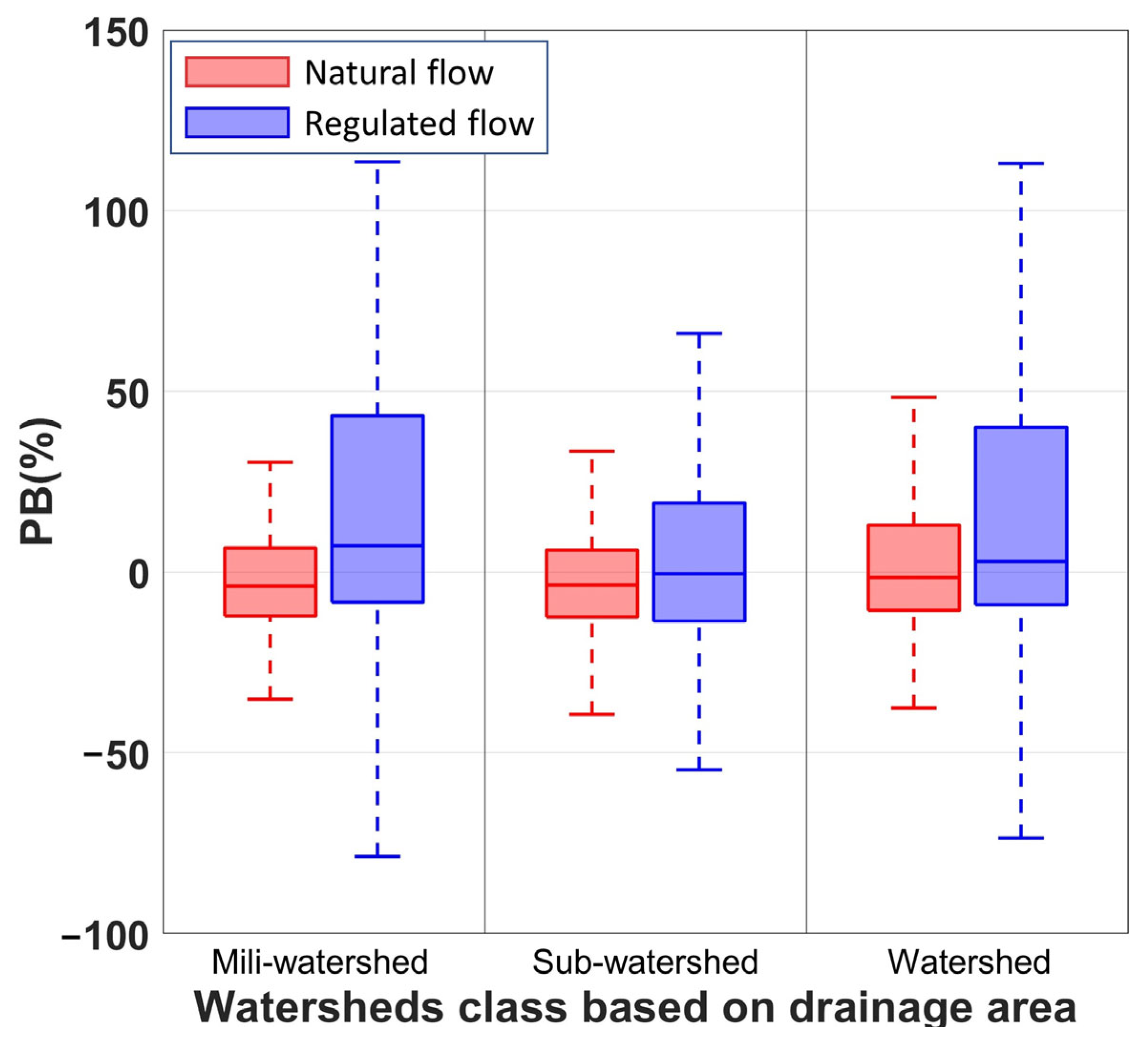
The performance of NWM streamflow estimates across different RFCs CONUS as a function of drainage areas was investigated. The watershed classification based on drainage area was derived from the classification scheme proposed by Singh (1994) [
55].
Figure 3 depicts the PB variation for distinct watershed classes across the CONUS. The results indicated a superior performance of the model in estimating streamflow for natural flow compared to regulated flow. Overall, the model exhibited a propensity for underestimating streamflow for Milli-watersheds (1000–10,000 ha) and sub-watersheds (10,000–50,000 ha) in natural flow estimates, with median PB values of −3.90% and −3.60%, respectively. Conversely, for the watershed class (>50,000 ha), the results demonstrated a lower median PB value of −1.51%, with the model tending to overestimate streamflow. In contrast, regulated flow outcomes displayed a suboptimal model performance with a broader spread in PB values. However, the model’s behavior was more stable for sub-watersheds, exhibiting a median PB value of −0.49% and a limited spread of obtained results (Q1 = −13.60, and Q3 = 19.06%). It is vital to note that the findings did not reveal any large-scale systematic bias in the model’s performance as a function of watershed drainage area. Consequently, to better characterize the model bias on a regional scale, the PB values for each RFC were extracted and analyzed individually.
PB results for each RFC as a function of drainage area are delineated in
Table 2 and
Table 3 for natural flow and regulated flow, respectively. The findings revealed that the model tends to underestimate natural flow in Milli-watersheds within the MARFC, NERFC, NWRFC, OHRFC, and SERFC. Conversely, the model exhibits a propensity to overestimate natural flow in Milli-watersheds situated in the MBRFC and CNRFC. For sub-watershed and watershed drainage basins, the model demonstrates a tendency to underestimate natural flow in the MARFC, NERFC, NCRFC, and OHRFC while overestimating natural flow in the MBRFC and CNRFC. The analysis suggests that NWM natural streamflow estimates are predominantly underestimated in eastern RFCs and overestimated in central RFCs, particularly for forecast points draining Milli-watersheds and sub-watersheds.
For regulated flow, the PB results exhibited less uniformity in bias distribution across various RFCs and drainage basin sizes. The outcomes indicated a propensity for the model to underestimate regulated flow over sub-watersheds and watersheds situated in the MARFC, NERFC, and OHRFC. Additionally, the results demonstrated a clear overestimation of streamflow in the MBRFC and CNRFC for different drainage basin sizes. The findings imply a random bias associated with streamflow estimates in regulated channels (
Table 3). These results can be attributed to both natural and anthropogenic alterations in the drainage basin environment that may not be accurately captured by the model due to static inputs such as land use/cover and catchment topography. Consequently, such changes may be more pronounced for smaller drainage basins where less consistency in the model behavior was observed.
A crucial aspect of the NWM’s performance lies in streamflow estimates as a function of stream order. In the present study, PB values corresponding to forecast points for different stream orders were analyzed. As depicted in
Figure 4, the PB values for natural flow estimates exhibit an approximately normal distribution, displaying a symmetrical distribution around the median and a relatively small interquartile range. It is also noteworthy that the PB values for natural flow series do not demonstrate significant skewness in any direction. Conversely, boxplots for the regulated flow outcomes indicate that PB values vary considerably as a function of stream order, exhibiting a substantial spread in IQR. The results also reveal high bias streamflow estimates obtained from first- and second-order regulated streams, suggesting a persistent bias associated with low-order regulated streams. The observed results can be attributed to the inherent assumptions related to channel properties in the NWM river network, including the adoption of trapezoidal channel geometry, uniform flow, and constant channel roughness that only varies depending on the stream order (up to 10 orders). These assumptions may influence flow routing and potentially introduce uncertainties in streamflow estimation that are order dependent. Additionally, the NWM employs the Noah–MP land surface model to simulate atmospheric exchanges with the surface and vertical fluxes within the soil moisture column at a 1-km grid resolution. Consequently, the model is anticipated to exhibit greater error generation in low order streams (small catchment), where the representation of channel infiltration may be insufficiently captured [
56]. This limitation underscores the need for further refinements in the model’s representation of channel properties and soil moisture distribution to improve streamflow predictions, particularly in small-scale drainage systems.
3.2. Temporal Analysis
The PB results were calculated for the NWM’s natural and regulated flow estimates in comparison with in-situ streamflow data. As shown in
Figure 5, a more favorable agreement between the estimated and observed streamflow data is achieved for natural flow across all 12 months of the year. For natural flow estimates, the results indicate that the model has a tendency to overestimate streamflow during the period between August and January, with median PB values greater than zero and a relatively positive skew in PB data. Natural flow estimates are predominantly underestimated during the period between March and June, with negative Q1 and median PB values, and Q3 values closer to 0. Higher negative PB values were obtained during March and April when seasonal transitions in streamflow regimes occur in most of the CONUS. The transition season coincides with snowmelt periods, which could be attributed to the NWM tendency to underestimate snow water equivalent (SWE). Conversely, the model’s positive bias during the wet season could be attributed to errors in precipitation inputs that trigger the generation of excess runoff.
The monthly variation of PB for regulated flow was assessed in this analysis. The PB for NWM estimates exhibited positive median values for all months, indicating a general propensity for the model to overestimate regulated flow (
Figure 5). The regulated flow estimates displayed enhanced performance during February and March, with median PB values closer to 0 and a relatively smaller IQR spread. Conversely, the results revealed the poorest PB values in July, August, and September, with median PB values of 23.90%, 27.37%, and 23.59%, respectively, and a large IQR spread, showcasing a tendency to overestimate streamflow. The larger PB values can be attributed to the fact that the NWM does not incorporate reservoir management practices. In other words, water retention in reservoirs is not represented in the model, which explains the substantial positive PB values.
3.3. Temporal–Spatial Analysis
The hourly streamflow data derived from the NWM retrospective simulation were contrasted with hourly in-situ streamflow data on a seasonal basis, taking into account the various climate zones encompassing the CONUS. It is crucial to acknowledge that the data utilized for the classification of climate zones could be influenced by the signal of climate change, as well as the impacts of teleconnections and climate variability, including the implications of diverse low-frequency climate oscillation indices at varying phases. This topic warrants substantial attention. However, the primary objective of the present research is to offer a preliminary delineation of the spatial distribution of aridity zones.
Regardless, the methodologies derived for climate zone classification align well with both regional and global studies that have explored the spatial variation of the Aridity Index [
57,
58]. Additionally, the findings of the current study correspond closely with those of Heidari et al. (2020) [
58]. Heidari et al. (2020) evaluated shifts in regional hydroclimatic conditions across the contiguous United States, in response to climate change throughout the 21st century. He generated Aridity Index maps for the period from 1989–2015, which exhibited patterns remarkably similar to those discerned in the present study [
58].
Figure 6 illustrates the spatiotemporal variation in the accuracy of the NWM natural flow estimates in terms of PB. In arid regions, the results revealed that the model generally overestimates streamflow values across all seasons, with median PB values of 7.85%, 18.80%, 19.54%, and 11.89% for fall, winter, spring, and summer estimates, respectively. These findings imply that the model exhibits enhanced performance during the summer and fall seasons in arid regions, while the performance deteriorates during the winter and spring seasons.
In semi-arid regions, the results indicated a favorable agreement between the model estimates and observed streamflow data during the spring season. In the remaining seasons, the model exhibited a tendency to overestimate streamflow, with median PB values exceeding zero and an IQR heavily skewed towards positive PB values. Streamflow estimates in semi-humid regions demonstrated a good correspondence with in-situ measurements, exhibiting a median PB value of 2.53%. The model displayed a clear inclination to overestimate streamflow during the winter season in the same region. Although the NWM streamflow estimates did not exhibit any systematic bias, the PB values were skewed in a positive direction.
The most favorable agreement between the NWM estimates and observed data was obtained for simulations conducted in humid regions. The results revealed low-bias error values with median PB values close to zero. The model’s best performance was observed during the winter season, potentially reflecting the model’s capability to generate accurate runoff during wet periods. It is worth noting that the model tends to underestimate streamflow during the spring season, which could be attributed to the model’s limitations in snowmelt-dominated regions.
Based on the results, it can be concluded that the accuracy of the NWM streamflow estimates is significantly influenced by seasonal streamflow variation. In semi-arid and sub-humid climate zones, the NWM streamflow estimates displayed good agreement with in-situ observations for spring season results. In humid regions, streamflow estimates were more accurate during fall and winter. For arid regions, the model demonstrated better agreement with in-situ observations during the fall season.
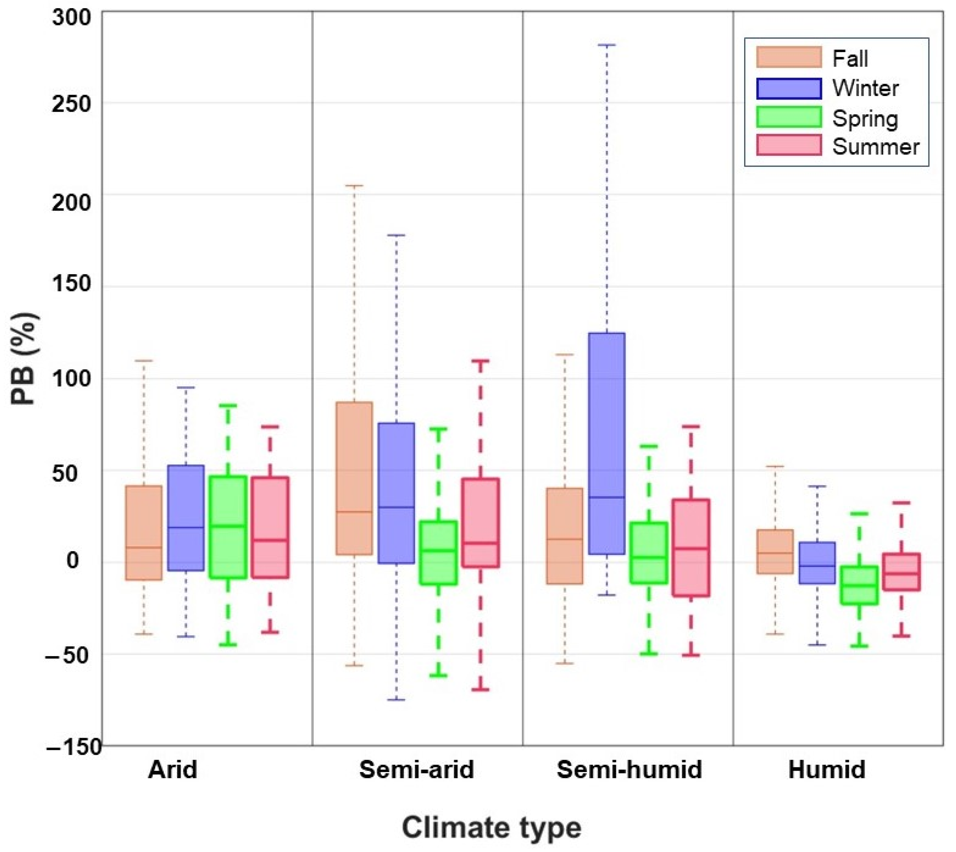
Figure 7 shows that, compared to natural flow, the NWM streamflow estimates for regulated flow exhibit lower accuracy in terms of PB for the different climate regions except humid areas. For instance, the median PB values for all seasons over the arid, semi-arid, and semi-humid regions obtained for natural flow simulations (
Figure 6) were remarkably lower than those obtained for the regulated flow simulations (
Figure 7). The NWM-regulated flow estimates yielded the poorest PB results, predominantly during the fall season, across most of the studied climate zones. The NWM regulated flow estimates demonstrated the most favorable agreement with in-situ measurements in humid regions, exhibiting low PB values throughout the various seasons. Conversely, the model performance deteriorated in arid regions, with a tendency to overestimate streamflow, as evidenced by positive Q1 and median PB values across different seasons. It is crucial to emphasize that, in semi-arid and sub-humid regions, the model error in terms of PB during the spring season was comparatively lower than in other seasons. The categorization of model PB results as a function of climate types across different seasons revealed a more distinct pattern in the spatial and temporal distribution of model error. For both natural and regulated flow simulations, the model exhibited commendable performance in streamflow estimation for humid and sub-humid regions. However, a diminished agreement between the simulated and observed streamflow was observed in arid and semi-arid regions.
The obtained results shown in
Figure 8 unveiled analogous streamflow trend patterns for the observed and simulated streamflow data from the years 1979 to 2020. The results showed a prevailing increasing trend in NERFC, MARFC, NCRFC, MBRFC, and MRRFC. Conversely, a dominant decreasing trend was observed in the western and southern portions of the CONUS, particularly for stations situated in the NWRFC, CNRFC, CBRFC, and WGRFC. However, this analysis primarily aims to compare results obtained from USGS streamflow records with NWM streamflow simulations. In the case of the NERFC, a significant discrepancy was observed between the MMK results for the in-situ observation series and the simulated series. The MMK outcomes for the NWM streamflow series exhibited a predominance of decreasing trends in the region, with 40% of the forecast point series revealing an opposing trend direction (decreasing trend) in comparison to the in-situ measurement trend direction (increasing trend). It is important to note that the NWM underestimated streamflow values for those simulations (negative PB values).
The opposite case was observed in parts of the SERFC, where in-situ observations disclosed a prevailing decreasing trend, while the NWM simulation displayed a dominant increasing trend. In those locations, PB results indicated a tendency of the model to overestimate streamflow. It is also pertinent to mention that distinct trend results for the NERFC and SERFC cases were discovered in forecast points within channels with a stream order of three or higher. The obtained results align with the findings presented in
Figure 4, where forecast points with higher stream order exhibited larger PB results, leading to an inadequate representation of the temporal evolution of streamflow in high-order streams.
For other RFCs where streamflow values were overestimated, such as the MBRFC, ABRFC, and WGRFC, trend results obtained from the NWM series demonstrated a dominant increasing trend in those regions. However, in-situ measurement results revealed a prevailing decreasing trend in the ABRFC and WGRFC. The obtained results could be elucidated by the positive PB and low correlation for forecast points located in these regions (
Figure 2c,i). Overall, the MMK test results disclosed a satisfactory agreement between the temporal evolution of the observed and simulated natural streamflow series for 74% of the studied dataset.
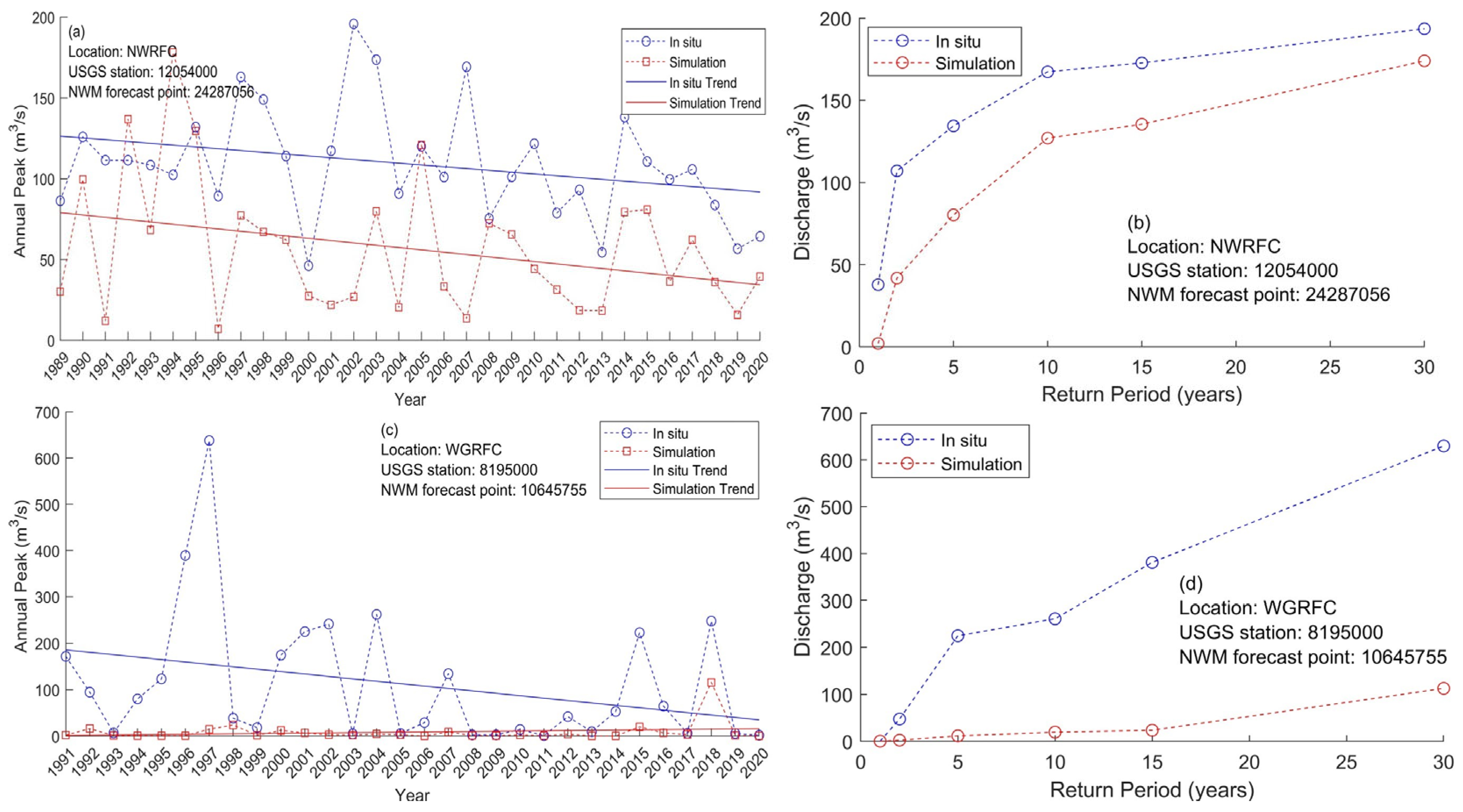
Regions exhibiting dominant negative streamflow trends and negative PB values pose significant concerns for products generated from the retrospective data, such as annual exceedance probability threshold values at forecast points, which are utilized to trigger flood inundation mapping in the operational NWM. To investigate this issue, we selected two representative stations with negative trends and negative PB values, characterized by close Z-MMK values, to retrieve the annual peak series and flood return periods. Initially, we extracted annual peak discharge from the daily streamflow time series and temporally matched these values with the corresponding values from the NWM simulations. It is crucial to note that the annual peak discharge values from the NWM simulation occurred within a 3-day time window of the USGS measurements, accounting for potential discrepancies in runoff generation lag time representation. In other words, within the same year, the NWM simulation could present a higher value than the selected value, which we consider a biased estimation of streamflow that could be attributed to biases in the forcing data.
As illustrated in
Figure 9, the annual peak series and flood return period demonstrate that, although the NWM simulation captures the trend of annual peak discharge values, there is a significant concern regarding the model’s representation of flood return periods. The 15-year return period flood value, which is used to trigger flood mapping in the operational model, is underestimated by the NWM simulation, as shown in
Figure 9b,d. This finding highlights the issue of the NWM underestimating peak flood values, necessitating bias correction of the NWM retrospective data. Several factors can contribute to the NWM model’s underestimation of peak discharge values. In addition to input data inaccuracies, model parameterization plays a substantial role in generating negative biases. Initial investigations into the source of the bias should primarily focus on land use and land cover data. The impact of updating the land use and land cover data while generating the retrospective dataset remains uncertain. Inaccurate land use and land cover data can lead to the misrepresentation of a catchment’s response to precipitation events, thereby causing an underestimation of peak discharge values. Furthermore, an incorrect representation of channel routing and floodplain storage can significantly impact the model’s ability to accurately simulate peak discharge values.
4. Discussion
In this study, the evaluation of the National Water Model retrospective data concentrated on the model’s streamflow estimation performance across the regional and temporal variations in the contiguous United States. The model bias and bias variation were scrutinized using multiple metrics, emphasizing percent bias (PB) variation for distinct climate classes. This approach facilitated a more standardized portrayal of the model’s performance across diverse climate regions.
In this section, we delve into the sources of uncertainty associated with the NWM streamflow simulation, encompassing input and output data, model structure, and model parameters. In the present study, the spatial analysis facilitated the delineation of underperforming catchments, predominantly situated along the high plains and desert southwest. The analysis of the spatial dispersion of model bias shows that regions characterized by elevated non-seasonal streamflow variability and frequent precipitation occurrences, such as the Southeast River Forecast Center and Northwest River Forecast Center, exhibited low variability errors. In contrast, arid and semi-arid regions demonstrated heightened variability errors. Catchments dominated by snowpack, including those within the Missouri Basin River Forecast Center, and areas with a more distinct seasonal cycle, such as the California–Nevada River Forecast Center, also revealed substantial variability errors.
It is widely acknowledged that hydrological models are susceptible to errors in hydrometeorological input data [
59]. Consequently, biases in forcing variables, particularly precipitation and near-surface air temperature, yield corresponding biases in model output. Lahmers et al. (2019) demonstrated that refining forcing data by integrating modeled atmospheric forcing with gauge-based precipitation measurements mitigated evapotranspiration biases and augmented the simulation of streamflow behavior [
60]. In a separate study, Viterbo et al. (2020) conducted an event-based model assessment and deduced that the NWM streamflow bias is influenced by both model errors and input errors [
61]. Furthermore, Garousi–Nejad and Tarboton (2022) identified a prevalent tendency for the NWM to underestimate Snow Water Equivalent (SWE) as a result of hydrologic process representation and hydrometeorological input errors [
62]. Their investigation revealed that the incorporation of observed precipitation and bias-corrected air temperature data ameliorated the general downward bias in NWM–SWE estimations. The model is also certainly sensitive to potential biases in soil moisture especially in watersheds with natural flow. The advent of satellite missions like the NASA SMAP that hold a potential to enhance streamflow forecast through data assimilation. This requires an exhaustive calibration and validation of the sensor’s estimates through various field campaigns [
63,
64].
For the NWM V2.1 retrospective simulations, the Analysis of Period of Record for Calibration (AORC) dataset was employed as forcing data. Although the blended product has high temporal and spatial resolutions and contains over a dozen individual rainfall datasets, there is need to evaluate the product performance over the CONUS while taking into account the seasonal variation of the product accuracy. For instance, Kim and Villarini (2022) assessed the AORC rainfall across Louisiana while focusing on the precipitation accuracy associated with Tropical Cyclone (TC) and non-TC conditions [
65]. The study showed that AORC performs better for the TC period compared to the non-TC ones. Thus, for regions with dominant small precipitation amounts, it is expected that the bias in AORC data would affect the soil condition and infiltration rates in the model simulation, as well as impact the water storage and the baseflow estimations. Hong et al. (2022) analyzed the AORC performance over the Great Lakes basin, and the analysis showed compared to 632 gauge stations, the product tends to overestimate daily precipitation and underestimate heavy rains with a notable larger bias value in cold months [
66]. The study also showed that the interannual change in AORC precipitation has divergent years while compared to other gridded precipitation products. To our knowledge, there are no continental scale assessments of AORC forcing hourly data, including precipitation, air temperature, specific humidity, surface pressure, radiation, and near-surface wind, which may have significant impact on accurately simulating evapotranspiration, snowmelt, and runoff generation processes. A better understanding of the NWM bias inherited from the forcing data would include the assessment of the AORC forcing.
The NWM performance is contingent upon the quality and accuracy of the static input data, which fundamentally represent catchment characteristics and significantly influence runoff generation, flow direction, and the configuration of the stream network. For instance, land use and land-cover data are crucial for determining the spatial distribution of vegetation, urban areas, and other surface types within a catchment, thereby directly impacting parameters associated with infiltration, evapotranspiration, and surface runoff generation. In the case of the NWM retrospective simulation, it is unclear which land cover dataset was used. However, the usage of static datasets similar to the retrospective runs of Versions 2.0 and 2.1 may result in biased simulations for periods when the used land cover layer does not match with the land cover of the simulation period. Similarly, using static soil data for a long-term simulation, encompassing properties such as texture, depth, and hydraulic conductivity, play a pivotal role in shaping infiltration capacity, water retention, and groundwater recharge processes throughout the catchment. Lastly, the accurate representation of river network and geometry, including parameters such as river width, depth, and slope, is indispensable for modeling flow routing and overland flow processes. For example, Ghanghas et al. (2022) assessed the reliability of Synthetic Rating Curves (SRC) across the CONUS by comparing them with the rating curves from USGS gauges [
67]. The identified errors in the SRC were attributed to topographical factors and inherent assumptions, such as employing reach-averaged channel properties, constant channel roughness, and uniform flow. These assumptions are consistent with those utilized in the NWM river network (NHDPlus). It is imperative to note that the NWM retrospective simulations serve as a basis for obtaining the 15-year return period flood discharge values across the CONUS. Subsequently, these discharge values are employed to initiate the flood inundation mapping process within the operational NWM framework. Consequently, inaccuracies in flood maps generated during forecasting may stem from errors in the estimated 15-year return period discharge values and/or the underlying SRC, emphasizing the importance of refining these components for improved flood prediction and mapping.
The uncertainty inherent in model streamflow simulations may also stem from errors in the in-situ measurements employed for model calibration and output assessment. While the gathered USGS streamflow data is verified through statistical and deterministic methods, such as flagging extreme discharge values, correlating independent observations, and conducting continuity tests, inherent errors in streamflow records may arise from alterations in stage–discharge relationships, backwater effects due to ice or debris, or equipment malfunctions. Thus, the correction of ice-affected streamflow is critical for evaluating models’ simulations in cold regions [
68]. Nevertheless, it is important to note that with advancements in estimating data uncertainty, the impact of such errors may be negligible. Conversely, it is imperative to emphasize that the NWM retrospective simulations scrutinized in this study do not incorporate streamflow observation nudging. As a result, the performance of the operational model version may be superior in localized areas where USGS observations are available. Despite this, the reported performance remains pertinent in identifying limitations in model parameterization and underlining the necessity for further refinement.
In this study, several key findings and recommendations emerge from the analysis of the model’s performance. First, it is evident that incorporating soil moisture data assimilation in humid regions, where frequent precipitation events are common, is essential to improve the model’s accuracy, as soil moisture dynamics play a crucial role in partitioning precipitation into runoff and infiltration, thereby directly impacting streamflow estimates. We would like to emphasize that the NWM’s soil moisture estimates are grid-based with a spatial resolution of 1 km. Consequently, a faithful representation of soil moisture within these grid cells would contribute substantially to a more accurate estimation of streamflow in such regions. In addition, it is also important to note that the operational version of the NWM actively nudging streamflow data from USGS stations. This nudging process is critical in updating the streamflow estimates within the model, but it does not affect the other hydrological components. Consequently, continuous and accurate soil moisture data assimilation would not only maintain the up-to-date status of soil moisture but also significantly enhance the model’s streamflow estimates, especially in predicting and managing flood events. These collective measures, in effect, would amplify the overall reliability and accuracy of the NWM’s streamflow estimates. Second, in cold regions, the assimilation of river ice data is necessary to better capture the effects of ice processes, such as freeze-up and break-up events, on streamflow dynamics, ultimately leading to more accurate predictions in these areas. Third, the uncertainty associated with the lack of knowledge regarding reservoir operation rules has been identified as a potential source of error in the model’s performance.
The challenges posed by river systems in the context of hydrological modeling necessitate a more sophisticated and adaptive approach. To tackle these complexities, we advocate for the exploration and integration of advanced computational methods, such as physics-informed machine learning and data mining, into the operational procedures of the NWM. Physics-informed machine-learning algorithms, which couple the power of data-driven models with the underlying physical principles governing the system, can provide insightful and reliable representations of reservoir operation rules. In this context, these techniques can help leverage the existing wealth of observational and operational data, enabling the extraction of complex relationships and patterns that traditional methods may struggle to discern. Moreover, enhancing the NWM’s capabilities through data-assimilation techniques could also significantly improve the simulation of streamflow estimates in regulated systems. Data assimilation, which blends model predictions with observed data to improve forecast accuracy and reduce uncertainty, has emerged as a powerful tool in hydrological modeling. Incorporating these inferred operation rules into the NWM would allow for a more faithful representation of the regulated systems, thereby significantly improving the accuracy of the model’s streamflow estimates. In this way, these advanced techniques could serve as catalysts in boosting the model’s overall performance, while simultaneously offering a more nuanced understanding of the hydrological processes at play in these regulated systems. These proposed recommendations, while demanding in terms of computational resources and methodological implementation, are projected to considerably enhance the capacity of the NWM to provide more reliable and accurate hydrological forecasts, ultimately benefiting a range of stakeholders in water resources management, flood prediction, and environmental conservation.
On the other hand, as we move towards the implementation of the Next Generation Modeling System (NextGen) for the National Water Model, opportunities for enhanced streamflow estimation, particularly in regions exhibiting poor performance with the current NWM, are anticipated [
69]. The NextGen framework, inherently model agnostic, offers immense flexibility, permitting the application of disparate methods or models to simulate specific hydrological fluxes. These simulations can be adjusted for diverse temporal and spatial scales, thereby accommodating unique hydrological characteristics across regions. The collaborative ethos embedded in the open-source philosophy of the NextGen framework augments methodological development within the scientific community. This atmosphere of collective engagement accelerates advancements in hydrological modeling techniques, promoting knowledge exchange and bolstering scientific growth. Moreover, this open-source approach empowers agencies to integrate proven models effectively within the NextGen framework, a feature that is notably advantageous for regions wherein certain models have demonstrated exceptional performance [
69]. Overall, the evolution towards the NextGen framework heralds a promising era for the NWM, offering pathways to surmount current limitations in streamflow estimation and substantially enhance the accuracy and reliability of hydrological predictions across the Continental United States. This transition signifies a noteworthy advancement in our ongoing journey towards comprehensive and adaptable hydrological modeling.


