Acquisition of Spatial and Temporal Characteristics of Shallow Groundwater Movement Based on Long-Term Temperature Time Series in the Kangding Area, Eastern Tibetan Plateau

Abstract

Heat has been widely used as a groundwater tracer to determine groundwater flow direction and velocity in a way that is ubiquitous, low-cost, environmentally friendly, and easy to use. However, temperature observations are generally short-term and small-scale, meaning they may not be able to reflect long-term changes in the characteristics of groundwater movement. In this study, we utilize 515 days of temperature data, collected from four measurement points in the Kangding area of the eastern Tibetan Plateau, in order to determine the spatial and temporal distribution of groundwater flow velocities using different analytical heat tracing methods. An analysis is conducted to evaluate the impact of thermal parameter uncertainties on the calculation of flow velocity, and a comparison is undertaken between the results of the phase, amplitude, and combined amplitude-phase methods. We subsequently discuss the relationship between flow velocity changes and precipitation. The results show that the estimated flow velocity is more susceptible to the volumetric heat capacity of the saturated sediment than it is to thermal conductivity. The phase method is more suitable for use in calculations in the study area, indicating that precipitation significantly impacts the flow velocity and that this impact is more pronounced in areas with flat terrain compared to areas with significant variation in elevation. Our research provides a comparative study of the heat tracing methods in areas with varied terrains and offers new evidence for the impact of precipitation and topography on groundwater infiltration.

1. Introduction

Quantifying groundwater fluxes to and from deep aquifers or shallow sediment is a critical task facing researchers from a variety of scientific disciplines, including hydrology, hydrogeology, climatology, and oceanography [1]. The traditional hydraulic method and isotope tracing method are commonly used for qualitative or quantitative estimations of groundwater migration characteristics. However, there are some limitations to these methods, including difficulties in accurately quantifying the hydraulic parameters, high monitoring costs, complex operations, and potential environmental pollution [2,3]. There is an urgent need for researchers to develop a low-cost, non-polluting, easy-to-use, and natural tracer method that can be monitored continuously. The movement of groundwater is always accompanied by heat transfer, resulting in significant disturbances of the temperature distribution under conditions of pure heat conduction. By utilizing the temperature profile variations with time, the direction and velocity of groundwater movement can be traced [1,4,5].

Early theoretical work in the 1960s showed that temperature measurements can be used in analytical solutions of the one-dimensional heat transport equation to solve for groundwater velocity [6,7]. Since then, researchers have conducted extensive research into the heat tracing method [5,8,9,10]. Hatch et al. proposed an analytical model for calculating groundwater flow velocities using the amplitude ratio and phase shift of periodic fluctuations in temperature at any two depths on a vertical profile [11]. Keery et al. [12] analyzed the temporal–spatial variability of water fluxes in the River Tern based on daily cycle variations in the temperature time series and proposed an analytical model for use in flux calculations. McCallum et al. [13] and Luce et al. [14] simultaneously used both the amplitude ratio and phase shift of the periodic temperature variations to calculate flow velocities. Later, Gordon et al. [15,16], on the basis of the above analytical solutions, published the MATLAB calculation program VFLUX which has since been widely used in water flux calculations. Most of these heat tracing studies have been based on diurnal temperature fluctuations that only exist <1 m, while only several studies have used annual cycle temperature data that could reach 20–30 m. Liu et al. [17] traced groundwater movement in a fault zone on the basis of annual temperature fluctuations at multiple measurement sites, providing new evidence for hydrothermal activity in the fault zone along the eastern margin of the Tibetan Plateau. Lu et al. [18] used continuous observations of bedrock temperature at multiple depths in the Kashgar region of Xinjiang, China, to obtain in situ thermal diffusivity measurements and shallow fluid transport characteristics. Chen et al. [19] compared the differences in the shallow flux exchange of a river after its calculation by VFLUX and 1DTempPro. They showed that temporal fluctuations and stratification in the temperature field and the hydrothermal exchange mainly occurred in the shallow region of the hyporheic zone. Previous studies have utilized temperature time series that mostly last for several or dozens of days and primarily focused on daily temperature fluctuations and small-scale infiltration characteristics. Long-term temperature records of multiple locations covering a sizeable area can assist in understanding regional groundwater movement differences over long timescales and in comparing the applicability of different heat tracing models.

This article estimates shallow groundwater flow velocities on the basis of a long time series and multi-site analysis. We use more than 500 days of high-precision bedrock temperature observations taken at four measurement points along the eastern margin of the Tibetan Plateau to estimate the groundwater flux via different analytical methods and compare their applicability in the study area. Then, the influence of precipitation and the geological environment on water fluxes are discussed. Overall, our study makes a comparative analysis of the heat tracing methods using long-term data, and offers insights into the effects of precipitation and topography on groundwater migration.

2. Data

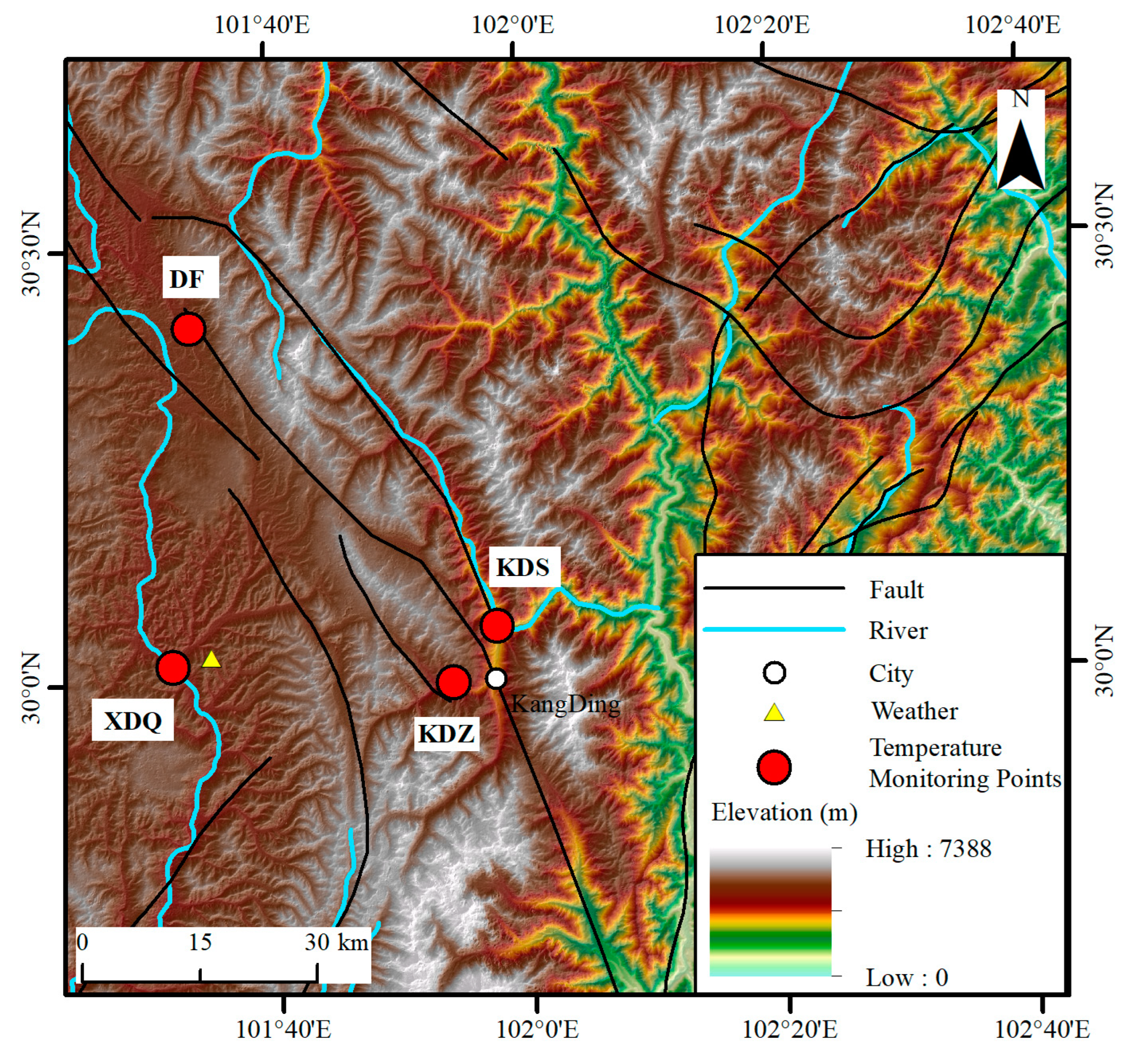
2.1. Station Information

The four temperature observation sites used in this study are located in the Kangding area near the Xianshuihe Fault Zone at the eastern margin of the Tibetan Plateau (Figure 1) and were constructed by the State Key Laboratory of Earthquake Dynamics [20]. The shallow groundwater in the fault zone is mainly bedrock fissure water, which is mostly recharged by atmospheric precipitation [21]. The river systems are in parallel with mountain chains and primarily flow southward. Under the influence of terrain and monsoon circulation, the area possesses a subtropical climate. Local meteorological records show that the annual temperature ranges from −14 °C to 28 °C, with an average of 8 °C [22].

The temperature data were recorded in a period from 1 February 2014 to 1 July 2015 (XDQ was recorded from 1 February 2014 to 10 September 2014). The XDQ measurement site is on the edge of a cliff at the foot of a mountain near the river. The KDS measurement site is at the foot of the mountain between the west side of the Goda Mountains and the east side of the Yala River, at a distance of about 25 m from the river. The KDZ measurement site is located on the west side of the Zeduo River, and the terrain descends from northwest to southeast near the monitoring site. The DF measurement site is near Heishi Mountain and is approximately 30 m from a tributary of the Xianshui River. The details of the stations are shown in

Table 1. Information about the temperature measurement stations in the study area.

Station	Town	Longitude (°E)	Latitude (°N)	Altitude (m)	Slope (°)
XDQ	Xinduqiao, Kangding	101.53	30.02	3419.0	17.34
KDS	Lucheng, Kangding	101.96	30.06	2460.5	12.92
KDZ	Zheduotang, Kangding	101.90	29.99	3084.0	8.32
DF	Zhonggu, Daofu	101.56	30.41	3626.3	9.47

Note: Slope information is calculated by ArcGIS.

.

2.2. Temperature Data

Temperature observations were carried out in 89 mm diameter boreholes using Pt1000 platinum resistance temperature sensors (Heraeus M222, 20NIPt10, class A, made in Germany). The sampling interval was 15 min, with a resolution of 0.0001 K [23]. Observations were made at 0 m, 0.25 m/0.3 m, 0.8 m, and 3.0 m/3.2 m depths (see Figure 2 for specific depths). The data were recorded using a data acquisition system and then sent to the data center via a wireless communication mode called the general packet radio service.

The shallow temperature in all the sites was characterized by apparent daily and annual cycles, with the temperature gradually increasing to a maximum from February to September and decreasing in the period from September to January. The daily variation of the temperature was evident at depths of 0 m, 0.25 m, and 0.3 m. Therefore, this study mainly used the daily cycle features of the temperature at 0 m, 0.25 m, and 0.3 m to obtain groundwater flow characteristics.

2.3. Precipitation Information

Under the influence of terrain and monsoon circulation, the area belongs to a subtropical climate. The precipitation data utilized in this study were obtained from the Kangding Weather Station, located at 101.58° E, 30.03° N (refer to Figure 1 for the location). The precipitation data showed that precipitation in the Kangding area was not high throughout the year (Figure 3). Mean annual precipitation was found to be 876.6 mm, the majority of which is concentrated between April and September.

3. Method of Analysis

3.1. Analytical Solutions for Obtaining Groundwater Flow Velocities Based on Periodic Temperature Fluctuations

The flow of groundwater is accompanied by heat transfer. Thus, by monitoring changes in temperature distribution, we can obtain the direction and velocity of the groundwater flow. Stallman presented the heat and water transport equation for a one-dimensional homogeneous porous medium [7]:

$$\begin{array}{l}\frac{\partial T}{\partial t}={{\displaystyle \kappa }}_e\frac{{\partial }^{2}T}{\partial z^2}-q\frac{C_w{\rho }_w}{C\rho }\frac{\partial T}{\partial z}\end{array}$$

(1)

where T is the temperature (°C), t is time (s), q is the velocity of the groundwater in the vertical direction (m s⁻¹), C_w is the volumetric heat capacity of water (J m⁻³ °C⁻¹), C is the volumetric heat capacity of the saturated sediment (J m⁻³ °C⁻¹), z is the depth (m), ρ is the density of water (kg/m³), ρ_w is the density of the saturated sediment (kg/m³), and κ_e is the equivalent thermal diffusivity of the saturated sediment, calculated as follows:

$${{\displaystyle \kappa }}_e=\frac{{\lambda }_0}{C}+\beta (\frac{C_w\left|q\right|}{C})$$

(2)

where λ₀ is the thermal conductivity of the saturated bulk medium (W m⁻¹ °C⁻¹), and β (m) is the thermal dispersion.

In the case of pure thermal conduction, the amplitude of the periodic temperature series decays exponentially with depth, and the phase is linearly delayed as heat transfers downwards from the surface. However, the groundwater movement can alter this pattern of amplitude and phase variation with depth compared to the conditions of pure thermal conduction [17,22,24]. Therefore, information on groundwater movement can be effectively determined by analyzing the amplitude and phase characteristics of periodic temperature variations at different depths.

Hatch et al. [11] derived an analytical solution for the quantitative calculation of vertical groundwater flow velocities in saturated porous media using the amplitude ratio or phase difference of temperature fluctuations at any two depths. The formula based on the amplitude ratio (A_r) is as follows:

$$q=\frac{C}{C_w}\left(\frac{2{\kappa }_e}{\mathrm{\Delta }z}\ln A_r+\sqrt{\frac{\alpha +v_t^2}{2}}\right)$$

(3)

where Δz is the sensor spacing, α is calculated by $\alpha =\sqrt{v_t^4+{(8\pi {\kappa }_e/P)}^2}$, P is the period of the temperature signal (s), and v_t is the velocity of the thermal front (m s⁻¹), which is defined as $v_t=\frac{qCw}{C}$. The formula based on the phase shift ($\Delta \varphi$) is as follows:

$$\left|q\right|=\frac{C}{C_w}\sqrt{\alpha -2{\left(\frac{4\pi \mathrm{\Delta }\varphi {\kappa }_e}{P\mathrm{\Delta }z}\right)}^2}$$

(4)

The amplitude method is most sensitive at low flow velocities, while the phase method continues to obtain relatively good results at high flow velocities. However, the phase-based method can only calculate the flow magnitude but cannot confirm the flow direction [11,25].

Later, Keery et al. [12] proposed another analytical solution for calculating groundwater flow velocity from the amplitude and phase of the periodic variations, where the formula based on the amplitude ratio (A_r) is as follows:

$$\left(\frac{H^3\ln A_r}{4\mathrm{\Delta }z}\right)q^3-\left(\frac{5H^2{\ln }^2{A}_r}{4\mathrm{\Delta }{z}^2}\right)q^2+\left(\frac{2H{\ln }^3{A}_r}{z^3}\right)q+\left(\frac{\pi C}{{\lambda }_{0}P}\right)-\frac{{\ln }^4{A}_r}{z^4}=0$$

(5)

The formula based on the phase shift ($\Delta \varphi$) is as follows:

$$\left|q\right|=\sqrt{{\left(\frac{C\mathrm{\Delta }z}{\mathrm{\Delta }\varphi C_w}\right)}^2-{\left(\frac{4\pi \mathrm{\Delta }\varphi {\lambda }_0}{P\mathrm{\Delta }z{C}_w}\right)}^2}$$

(6)

where $H=C_w/{\lambda }_0$. Just as occurred with the model of Hatch et al. [11], the phase-based approach in the model of Keery et al. [12] failed to identify the flow direction. However, unlike the approach of Hatch et al. [11], this model did not incorporate consideration of thermal dispersivity. In addition, Keery et al. [12] quantified the spatial and temporal variability of groundwater flow velocities on the basis of temperature time series analysis using dynamic harmonic regression (DHR) signal processing techniques.

McCallum et al. [13] derived a method for calculating the vertical groundwater flow velocity by combining the amplitude and phase of temperature changes:

$$q=-\frac{C}{C_w}\left(\frac{\mathrm{\Delta }z\left(P^2{\ln }^2{\mathrm{A}}_r-4{\pi }^2\mathrm{\Delta }{\varphi }^2\right)}{\mathrm{\Delta }\varphi \sqrt{16{\pi }^4\mathrm{\Delta }{\varphi }^4+8P^2{\pi }^2\mathrm{\Delta }{\varphi }^2{\ln }^2{A}_r+P^4{\ln }^4{A}_r}}\right)$$

(7)

This method allows the equivalent thermal diffusivity of the medium to be calculated simultaneously. Its use, therefore, does not require a priori knowledge of the thermal conductivity of the medium, which is an advantage over the previous two models. Furthermore, the method of McCallum et al. [13] has the potential to be used in the detection of erroneous data in the temperature time series based on anomalies in the temporal variation of the thermophysical parameters. However, using the method may result in significant errors under transient flux conditions, but it works well in low-flux regions (e.g., <0.1 m/d) and at points where the thermal parameters are uncertain [13,25].

VFLUX2 is a program designed to calculate groundwater flow velocity based on one-dimensional heat transport equations. Developed by the models of Hatch et al. [11], Keery et al. [12], McCallum et al. [13], and Luce et al. [14], this was the primary program used in this study. The daily cycle temperature fluctuations at depths of 0 and 0.3 m (0.25 m in the KDZ) were used in the calculations of this study. The thermal physical parameters of the soil were referenced by Lapham [26] and Fetter [27].

Table 2. Parameters for flow velocity calculation.

Parameter	Value
Porosity, n	0.28
Dispersivity, m	0.001
Volumetric heat capacity of the sediment, C (J m−3 °C−1)	2.09 × 106
Volumetric heat capacity of the water, Cw (J m−3 °C−1)	4.18 × 106
Thermal conductivity of the sediment, λ0 (w m−1 °C−1)	1.88

contains the specific parameter settings.

3.2. Data Processing Methods

3.2.1. Data Completion

Temperature records of long time series usually encounter issues with missing data. Among the observations in this calculation, the temperature data at the DF and KDS sites were missing for up to 6 h, an issue which mainly occurred around midnight. By comparing the trends before and after the missing periods, linear variation was found to be prominent during this period. Consequently, a linear interpolation method was used to complete the missing data [28].

3.2.2. Noise Reduction

The temperature observation data are often contaminated with various types of noise, which can lead to errors in the subsequent analysis. We employed a one-dimensional discrete wavelet analysis method to address this issue and filtered out high-frequency random noise with periods below three hours from the raw temperature time series [29]. This filter helped to reduce the noise level and improve the accuracy of our calculation.

3.2.3. Daily Precipitation Data Processing

Ground temperature monitoring in this study mainly covered the foothill areas, which feature a gentle terrain. The precipitation events could influence subsequent infiltration [30]. In order to undertake comparisons with the calculated groundwater flow velocities, we used the average precipitation of the previous three days as the current day’s precipitation reference value. This approach was adopted to consider the impact of earlier precipitation on the current day’s groundwater movement without altering the precipitation trend or affecting the subsequent trend analysis.

4. Results

4.1. Transient Changes in Groundwater Flow Velocities

The calculated groundwater flow velocities and their relationship with precipitation at the four measurement sites in the Kangding area are shown in Figure 4. As there was little difference between the results calculated by the models of Hatch et al. [11] and Keery et al. [12] in terms of the phase shift or amplitude ratio methods, only the amplitude-based data from the work of Hatch et al. [11] and the phase-based data from Keery et al. [12] were used for the comparison of the calculation results.

The mean groundwater flow velocities of the XDQ, KDS, KDZ, and DF measurement points obtained via the phase method were 1.26 × 10⁻⁵, 5.89 × 10⁻⁶, 7.35 × 10⁻⁶, and 7.85 × 10⁻⁶ m s⁻¹. The mean values of the flow velocities calculated via the amplitude method were 3.35 × 10⁻⁶, 4.57 × 10⁻⁷, 6.99 × 10⁻⁷, and 2.12 × 10⁻⁶ m s⁻¹ for the XDQ, KDS, KDZ, and DF measurement points. The results calculated by the combined amplitude-phase method were 1.38 × 10⁻⁶, 1.06 × 10⁻⁶, 1.72 × 10⁻⁶, and 1.28 × 10⁻⁷ m s⁻¹ for the four measurement points. The results show that the groundwater flow velocities calculated by the phase and combined amplitude-phase methods at the XDQ site vary significantly during the rainy season, with several peaks occurring between April and October, followed by gentle flow velocities between November and February, while the results from the amplitude method are relatively smooth overall (Figure 4a). Overall, the results obtained from the KDS site using the phase method and the combined amplitude-phase method show similar trends. The flow velocity increases in May and then decreases in June and July, followed by several peaks from July to October, and becomes almost stable from November to February. However, the flow velocity, as calculated via the amplitude method, generally remains steady (Figure 4b). The groundwater flow at the KDZ site shows a significant fluctuation in velocity, with significantly changed velocity in June and July each year for all the methods. However, during the rainy season, using the amplitude method results in lower velocities, whereas employing the phase and combined amplitude-phase methods show higher velocities (Figure 4c). The results of the three methods were similar during the short period during which the DF site was observed, with peak velocities between June and September, but gentle changes for the remaining time (Figure 4d).

4.2. Uncertainty Analysis

The thermal parameters for calculating groundwater flow rates in the study were quoted from the literature. There were potentially some uncertainties in this information, which would lead to errors in flow rate calculations. Therefore, it was necessary to investigate the influence of the thermal parameter uncertainties on the calculation results [2,8,24,31,32]. In order to analyze the influence of the uncertainty in the thermal parameters on the results, we took the XDQ site as an example on which to carry out uncertainty analysis for the two thermal parameters, namely, the volumetric heat capacity and thermal conductivity of the saturated sediment.

Firstly, we reduced and increased the thermal conductivity by 10% relative to the reference value (i.e., 1.692 and 2.068 (W m⁻¹ °C⁻¹)). The calculated results were compared with the results in Section 4.1, shown in Figure 5.

As the thermal conductivity changed, the flow velocity calculated using phase and amplitude methods fluctuated to a small extent. However, the trend in flow velocity did not change. The results of the combined amplitude-phase method did not change with the thermal conductivity, which is consistent with the fact that the model of McCallum et al. [13] does not rely on thermal conductivity. As can be seen from the analysis, the uncertainty in the thermal conductivity does not change the trend in flow velocity. While it does, cause a slight fluctuation in the magnitude of the calculated flow velocity, this has little effect on our trend analysis.

Subsequently, we reduced and increased the saturated sediment volumetric heat capacity by 10% relative to the reference value (i.e., 1.8819 × 10⁶ and 2.3001 × 10⁶ (J m⁻³ °C⁻¹)) to compare with the results in Section 4.1.

As can be seen from the results above (Figure 6), changing the sediment volumetric heat capacity affects the results of the case of flow velocity for all the methods. The effect is particularly significant for the amplitude method. However, similar to the thermal conductivity, changing the volumetric heat capacity does not affect the trend of the flow velocity variations or significantly affect the subsequent analysis. The effect of sediment volumetric heat capacity on the calculations is greater than that of thermal conductivity. Overall, the flow velocity calculated using the combined amplitude-phase method is minimally impacted by the thermal physical parameters.

5. Discussion

5.1. Comparison of Flow Velocity Calculation Methods

This article used three models (amplitude ratio, phase shift, combined amplitude-phase) to calculate the groundwater flow velocity in the study area. In this study, we compared the results from different methods. The high-altitude Kangding area possesses a complex geological environment and continually displays both a variety of faults in the surrounding area and frequent fluid activity. From the calculation results, it can be asserted that the groundwater flow velocities at all four measurement points are relatively high (>0.1 m/d), meaning that the amplitude and combined amplitude-phase methods may not have good sensitivity to flow velocity variations. The overall trend in the results of these two methods is relatively gentle and does not illustrate the impact of precipitation, meaning that it may not accurately reflect the groundwater flow conditions. On the other hand, the phase method is more sensitive to higher flow velocities and more accurate at high flow velocities than the other methods, giving it a unique advantage in areas of high flux [25]. However, the phase method can only be used to estimate the magnitude but not the direction of the flow, as shown in Equation (4). The calculations in this article also show that the phase method obtains more significant changes in groundwater seepage velocities during the rainy season. Overall, the results calculated by the amplitude method are comparable to those of the combined amplitude-phase method, overall yielding more reliable results at a low flow velocity. The phase method obtains a flow velocity with greater fluctuation. It seems that the phase method is more effective when used to conduct a long-term trend analysis of the four high flow velocity sites in this study.

5.2. Comparison of Flow Velocities and Precipitation

There are two primary perspectives on the effect of precipitation on infiltration. The first view is that heavy precipitation causes an enormous rush of rainwater, resulting in an effective infiltration rate [33,34]. The other view is that the disintegration of soil aggregates by rainwater impact and concentration of translocated silt and clay particles creates a dense layer immediately below the surface, resulting in a lower infiltration rate [35,36]. Both views are somewhat applicable, with differences in the study areas leading to different conclusions [37]. The greater the depth and the smaller the groundwater flow velocity, the less effective the temperature is at portraying the groundwater flow velocity [38]. The data used in this study were mainly observed at depths of 0 m, 0.25 m, and 0.3 m, meaning points that belong to shallow groundwater in depth. The relationship between precipitation and infiltration can be reflected in the groundwater flow velocity [39,40].

The results of the flow velocities calculated by the phase method show that during times of significantly increased precipitation, such as 1 April 2014, 27 August 2014, 3 September 2014, and 17 May 2015, the groundwater flow velocities at XDQ, DF, and KDS corresponded to several peaks compared to other times. In contrast, from December 2014 to March 2015, when there was almost no precipitation, there was no significant change in groundwater flow velocities. Even at the KDZ measurement site, where the peaks in precipitation and flow velocity did not coincide very well, flow velocities were gentle when there was no precipitation. We can thus conclude that, although there is no strict one-to-one correspondence between the two, precipitation affects shallow groundwater flow velocity.

5.3. Comparison of Flow Velocities and Topography

Some tests have shown that groundwater infiltration decreases as the slope increases [41,42,43,44,45,46,47]. Zhu et al. showed that each effect factor on the seepage field plays the strongest role on the slope toe, a weaker role on the middle part of the slope, and the weakest role on the top slope [48]. Hou et al. found that the infiltration is more sensitive to the 0° to 5° slope than to the 5° to 10° slope [46]. Some studies indicated no relationship between slope and infiltration. Hao et al. conducted artificial rainfall experiments, showing that infiltration rate does not demonstrate obvious differences between different slopes [44]. It can be seen that the different methods and experimental conditions used result in different conclusions [49]. Thus, it is necessary to discuss different areas specifically. Our analysis of the topography and flow velocity for the four measurement points shows that (Figure 7), with the exception of the KDZ measurement point, the infiltration at the other points correlated with the slope. The XDQ site is close to the river and located at the foot of the hill, with gentle terrain on one side facilitating rainwater retention and significant flow velocity increasing responses to precipitation. The KDS site is located at the confluence of the river, with high terrain on all sides and low land in the middle. These factors may lead to a long rainwater retention time and a significant effect of precipitation on groundwater flow velocities. The DF site is at the highest elevation but is behind the Black Rock Mountain, with the Xianshui River flowing nearby. The surrounding terrain is gentle, meaning that precipitation has a long retention time and significantly affects groundwater flow velocities. However, the KDZ site is located halfway up the hill, and the river flows from west to east near the point and does not converge with it, showing a significantly different environment from the other areas assessed. Therefore, the impact of precipitation on the groundwater flow velocity at this measuring point would be much smaller than that of other measuring points. In addition, the raw data of the KDZ site show that the fluctuations in shallow ground temperature are very pronounced compared to the other three sites, which directly contributes to the wide range of fluctuations in the flow velocity.

In summary, the differences in flow velocities among the four measurement sites are likely primarily related to their geographical location. Areas with low and gentle topography, where rainwater is retained for extended periods, more significantly affect groundwater flow velocities than areas with high and steep topography.

6. Conclusions

In this study, the groundwater flow velocity variations in four measurement sites in the Kangding area at the southeastern edge of the Tibetan Plateau were obtained from long-term (515-day) temperature observations. We compared the calculated flow velocity using several analytical heat tracing models and analyzed the impact of thermal parameter uncertainties on the results. The influences of precipitation and topography on the flow velocity were discussed. The key findings can be summarized as follows:

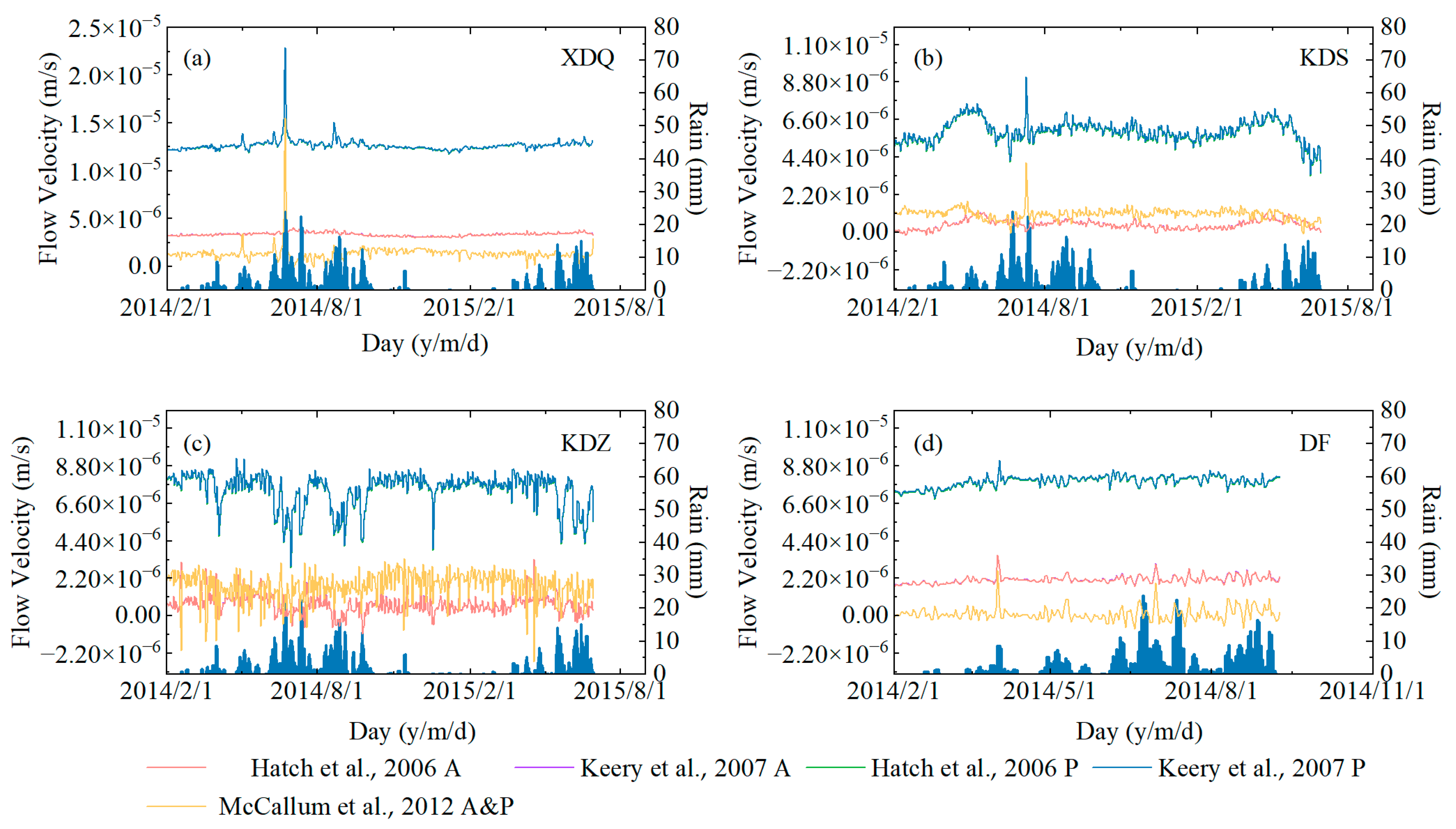
• The groundwater flow velocities at all four measurement points are relatively high, being in the order of 10⁻⁶~10⁻⁵ m s⁻¹. The phase method is more suitable for use in the calculation in these areas because of its sensitivity to changes in high flow velocity. However, the phase method can only be used to estimate the magnitude and cannot distinguish the direction of the flow. The results of the amplitude method are comparable to those of the combined amplitude-phase method, with an overall gentle variation in flow velocity and no significant changes after the precipitation.
• The results show that the estimated flow velocity is more influenced by the volumetric heat capacity of the saturated sediment than thermal conductivity, but the uncertainties in the thermal parameters do not affect the flow trend. The results of the combined amplitude-phase method are relatively insusceptible to thermal parameters compared to the phase and amplitude methods.
• The results show a clear relationship between groundwater flow velocity variation and local precipitation in the Kangding area. The stronger the precipitation, the higher the flow velocity of shallow groundwater. When the precipitation is low, there is almost no significant fluctuation in groundwater flow velocity.
• The variation in groundwater flow velocities at the four measurement sites may be affected by the topography, as the topography can influence the duration of rainwater retention. Gentle terrain has a higher tendency to retain rainfall, a factor which, combined with the water gathering from surrounding rivers, significantly affects groundwater flow velocities (e.g., XDQ, KDS, and DF). Conversely, areas with high relief are less susceptible to rainwater retention, and the infiltration velocity does not vary significantly after precipitation (e.g., KDZ).

References

1. Kurylyk, B.L.; Irvine, D.J.; Bense, V.F. Theory, tools, and multidisciplinary applications for tracing groundwater fluxes from temperature profiles. WIREs Water 2018, 6, e1329. [Google Scholar] [CrossRef] [Green Version]
2. Rau, G.C.; Andersen, M.S.; McCallum, A.M.; Roshan, H.; Acworth, R.I. Heat as a tracer to quantify water flow in near-surface sediments. Earth-Sci. Rev. 2014, 129, 40–58. [Google Scholar] [CrossRef] [Green Version]
3. Ma, R.; Dong, Q.; Sun, Z.; Zheng, C. Using heat to trace and model the surface water-groundwater interactions: A review. Geol. Sci. Technol. Inf. 2013, 32, 131–137. (In Chinese) [Google Scholar]
4. Dong, L.Y.; Chen, J.Y.; Shimada, J.; Yin, Z.X. Research Progress of Heat as a Tracer to Interpret Scientific Problems in Hydrogeology. J. Yangtze River Sci. Res. Inst. 2018, 35, 39–45. (In Chinese) [Google Scholar]
5. Anderson, M.P. Heat as a ground water tracer. Ground Water 2005, 43, 951–968. [Google Scholar] [CrossRef]
6. Bredehoeft, J.D.; Papaopulos, I. Rates of vertical groundwater movement estimated from the Earth’s thermal profile. Water Resour. Res. 1965, 1, 325–328. [Google Scholar] [CrossRef]
7. Stallman, R. Steady one-dimensional fluid flow in a semi-infinite porous medium with sinusoidal surface temperature. J. Geophys. Res. 1965, 70, 2821–2827. [Google Scholar] [CrossRef]
8. Constantz, J.; Cox, M.H.; Su, G.W. Comparison of heat and bromide as ground water tracers near streams. Groundwater 2003, 41, 647–656. [Google Scholar] [CrossRef]
9. Goto, S.; Yamano, M.; Kinoshita, M. Thermal response of sediment with vertical fluid flow to periodic temperature variation at the surface. J. Geophys. Res. Solid Earth 2005, 110, B01106. [Google Scholar] [CrossRef]
10. Taniguchi, M.; Shimada, J.; Tanaka, T.; Kayane, I.; Sakura, Y.; Shimano, Y.; Dapaah-Siakwan, S.; Kawashima, S. Disturbances of temperature-depth profiles due to surface climate change and subsurface water flow: 1. An effect of linear increase in surface temperature caused by global warming and urbanization in the Tokyo Metropolitan Area, Japan. Water Resour. Res. 1999, 35, 1507–1517. [Google Scholar] [CrossRef]
11. Hatch, C.E.; Fisher, A.T.; Revenaugh, J.S.; Constantz, J.; Ruehl, C. Quantifying surface water-groundwater interactions using time series analysis of streambed thermal records: Method development. Water Resour. Res. 2006, 42, W10410. [Google Scholar] [CrossRef] [Green Version]
12. Keery, J.; Binley, A.; Crook, N.; Smith, J.W.N. Temporal and spatial variability of groundwater–surface water fluxes: Development and application of an analytical method using temperature time series. J. Hydrol. 2007, 336, 1–16. [Google Scholar] [CrossRef]
13. McCallum, A.M.; Andersen, M.S.; Rau, G.C.; Acworth, R.I. A 1-D analytical method for estimating surface water-groundwater interactions and effective thermal diffusivity using temperature time series. Water Resour. Res. 2012, 48, WR012007. [Google Scholar] [CrossRef]
14. Luce, C.H.; Tonina, D.; Gariglio, F.; Applebee, R. Solutions for the diurnally forced advection-diffusion equation to estimate bulk fluid velocity and diffusivity in streambeds from temperature time series. Water Resour. Res. 2013, 49, 488–506. [Google Scholar] [CrossRef] [Green Version]
15. Gordon, R.P.; Lautz, L.K.; Briggs, M.A.; McKenzie, J.M. Automated calculation of vertical pore-water flux from field temperature time series using the VFLUX method and computer program. J. Hydrol. 2012, 420–421, 142–158. [Google Scholar] [CrossRef]
16. Gordon, R.P.; Lautz, L.K.; Daniluk, T.L. Spatial patterns of hyporheic exchange and biogeochemical cycling around cross-vane restoration structures: Implications for stream restoration design. Water Resour. Res. 2013, 49, 2040–2055. [Google Scholar] [CrossRef]
17. Liu, Q.Y.; Chen, S.Y.; Jiang, L.W.; Wang, D.; Yang, Z.Z.; Chen, L.C. Determining thermal diffusivity using near-surface periodic temperature variations and its implications for tracing groundwater movement at the eastern margin of the Tibetan Plateau. Hydrol. Process. 2019, 33, 1276–1286. [Google Scholar] [CrossRef]
18. Lu, L.L.; Chen, S.Y.; Liu, Q.Y.; Yan, W.; Liu, P.X.; Song, C.Y.; Feng, J.H.; Chen, L.C. Determining groundwater movement from bedrock temperature: A case study of Kashi area. Chin. J. Geophys. 2021, 64, 4594–4606. (In Chinese) [Google Scholar]
19. Chen, J.Q.; Ren, J.; Ni, F.; Wang, D.B. Quantitative Study on Exchange Flux of Undercurrent in Riverbed Based on 1DtempPro and VFLUX. Water Resour. Power 2021, 39, 37–40. (In Chinese) [Google Scholar]
20. Chen, S.Y.; Liu, P.X.; Liu, L.Q.; Ma, J. A phenomenon of ground temperature change prior to Lushan earthquake observed in Kangding. Seismol. Geol. 2013, 35, 634–640. (In Chinese) [Google Scholar]
21. Zhang, Y.H.; Xu, M.; Li, X.; Qi, J.H.; Zhang, Q.; Guo, J.; Yu, L.L.; Zhao, R. Hydrochemical characteristics and multivariate statistical analysis of natural water system: A case study in Kangding County, Southwestern China. Water 2018, 10, 80. [Google Scholar] [CrossRef] [Green Version]
22. Liu, Q.Y.; Chen, S.Y.; Chen, L.C.; Liu, P.X.; Yang, Z.Z.; Lu, L.L. Detection of groundwater flux changes in response to two large earthquakes using long-term bedrock temperature time series. J. Hydrol. 2020, 590, 125245. [Google Scholar] [CrossRef]
23. Zhang, Z.H.; Chen, S.Y.; Liu, P.X. A key technology for monitoring stress by temperature: Multichannel temperature measurement system with high precision and low power consumption. Seismol. Geol. 2018, 40, 499–510. [Google Scholar]
24. Constantz, J. Heat as a tracer to determine streambed water exchanges. Water Resour. Res. 2008, 44, W10D. [Google Scholar] [CrossRef]
25. Irvine, D.J.; Lautz, L.K.; Briggs, M.A.; Gordon, R.P.; McKenzie, J.M. Experimental evaluation of the applicability of phase, amplitude, and combined methods to determine water flux and thermal diffusivity from temperature time series using VFLUX 2. J. Hydrol. 2015, 531, 728–737. [Google Scholar] [CrossRef] [Green Version]
26. Lapham, W.W. Use of temperature profiles beneath streams to determine rates of vertical ground-water flow and vertical hydraulic conductivity. US. Geol. Surv. Water Supply Pap. 1989, 2337, 1–35. [Google Scholar]
27. Fetter, C.; Fetter, C. Applied Hydrogeology; Prentice Hall: Upper Saddle River, NJ, USA, 2001; pp. 17–598. [Google Scholar]
28. Soltani, A.; Meinke, H.; De Voil, P. Assessing linear interpolation to generate daily radiation and temperature data for use in crop simulations. Eur. J. Agron. 2004, 21, 133–148. [Google Scholar] [CrossRef]
29. Poularikas, A.D.; Ramadan, Z.M. Adaptive Filtering Primer with MATLAB; CRC Press: Boca Raton, FL, USA, 2017. [Google Scholar]
30. Zhang, C.L.; Li, P.; Li, T.L.; Zhang, M.S. In-situ observation on rainfall infiltration in loess. J. Hydraul. Eng. 2014, 45, 728–734. (In Chinese) [Google Scholar] [CrossRef]
31. Gao, Z.Q.; Lenschow, D.H.; Horton, R.; Zhou, M.Y.; Wang, L.L.; Wen, J. Comparison of two soil temperature algorithms for a bare ground site on the Loess Plateau in China. J. Geophys. Res. Atmos. 2008, 113, D18105. [Google Scholar] [CrossRef] [Green Version]
32. Shanafield, M.; Hatch, C.; Pohll, G. Uncertainty in thermal time series analysis estimates of streambed water flux. Water Resour. Res. 2011, 47, W03504. [Google Scholar] [CrossRef]
33. Shi, S.X. A testing study of factors affecting infiltration rate under artificial rainfall with high intensity. Bull. Soil Water Conserv. 1992, 12, 49–54. (In Chinese) [Google Scholar]
34. Zhao, X.N.; Wu, F.Q.; Wang, W.Z. Research on soil infiltration law of slope farmland in Gully Area of Loess Plateau. J. Arid. Land Resour. Environ. 2004, 18, 109–112. (In Chinese) [Google Scholar]
35. Helalia, A.M.; Letey, J.; Graham, R.C. Crust Formation and Clay Migration Effects on Infiltration Rate. Soil Sci. Soc. Am. J. 1988, 52, 251–255. [Google Scholar] [CrossRef]
36. Morin, J.; Van Winkel, J. The Effect of Raindrop Impact and Sheet Erosion on Infiltration Rate and Crust Formation. Soil Sci. Soc. Am. J. 1996, 60, 1223–1227. [Google Scholar] [CrossRef]
37. Lv, G.; Wu, X.Y. Review on influential factors of soil infiltration characteristics. Chin Agric. Sci. Bull. 2008, 24, 494–499. (In Chinese) [Google Scholar]
38. Pan, W.Y.; Yang, S.S.; Liu, J.F.; Qian, X.H.; Xu, Z.H. Research on the Groundwater Flow Rate during the River Hyporheic Layer Based on the Temperature Tracer. China Rural. Water Hydropower 2023, 2, 121–127. (In Chinese) [Google Scholar]
39. Wu, J.Q.; Zhang, R.D.; Yang, J.Z. Analysis of rainfall-recharge relationships. J. Hydrol. 1996, 177, 143–160. [Google Scholar] [CrossRef]
40. Li, Y.F.; Li, X.F. Study on precipitation infiltration recharge with groundwater depth variation. J. China Hydrol. 2007, 27, 58–60. (In Chinese) [Google Scholar]
41. Jiang, D.; Huang, G. Simulation experiment on the effect of slope gradient on rainfall infiltration. Bull. Soil Water Conserv. 1984, 4, 10–13. (In Chinese) [Google Scholar]
42. Wu, S.F. Study on the Effect and Mechanism of the Slope Runoff Regulation; Northwest A&F University: Xianyang, China, 2006. [Google Scholar]
43. Cerdà, A. Seasonal variability of infiltration rates under contrasting slope conditions in southeast Spain. Geoderma 1996, 69, 217–232. [Google Scholar] [CrossRef] [Green Version]
44. Hao, C.H.; Pan, Y.H.; Cheng, X.; Cui, S.F. Influence of slope and rainfall intensity on infiltration characteristics of Lou Soil. Chin. J. Soil Sci. 2011, 42, 1040–1044. (In Chinese) [Google Scholar]
45. Khaerudin, D.N.; Suharyanto, A.; Harisuseno, D. Infiltration Rate for Rainfall and Runoff Process with Bulk Density Soil and Slope Variation in Laboratory Experiment. Nat. Environ. Pollut. Technol. 2017, 16, 219–224. [Google Scholar]
46. Hou, J.; Zhang, Y.; Tong, Y.; Guo, K.; Qi, W.; Hinkelmann, R. Experimental study for effects of terrain features and rainfall intensity on infiltration rate of modelled permeable pavement. J. Environ. Manag. 2019, 243, 177–186. [Google Scholar] [CrossRef] [PubMed]
47. Huang, M.B.; Li, Y.S.; Kang, S.Z. Analysis of unit rainfallrunoff theory and calculation of average infiltration ration on slope land. J. Soil Erosion Soil Water Conserv. 1999, 5, 63–68. (In Chinese) [Google Scholar]
48. Zhu, Z.Y.; Zhang, F.; Ling, X.Z.; Huang, M.Q.; Li, Q.L. Rainfall-induce Seepage Field of a High Slope and Its Effect Factors. Adv. Mater. Res. 2011, 243, 2423–2428. [Google Scholar]
49. Morbidelli, R.; Saltalippi, C.; Flammini, A.; Govindaraju, R.S. Role of slope on infiltration: A review. J. Hydrol. 2018, 557, 878–886. [Google Scholar] [CrossRef]
Figure 1. Distribution of the temperature measurement stations. DEM data source: https://www.gscloud.cn/ (accessed on 1 April 2023), 30 m resolution.
Water 15 02140 g001
Figure 2. Raw temperature records of the measurement stations.
Water 15 02140 g002
Figure 3. Daily precipitation.
Water 15 02140 g003
Figure 4. Groundwater flow velocities calculated for the measurement points using different methods. The blue bars in the graph show the average precipitation values for the previous three days. The red and purple curves show the results of the amplitude method of Hatch et al. [11] and Kerry et al. [12]. The green and blue curves show the results of the phase method of Hatch et al. [11] and Kerry et al. [12]. The yellow curves show the combined amplitude and phase method of McCallum et al. [13].
Water 15 02140 g004
Figure 5. Uncertainties in flow velocity estimation resulting from the uncertainty in thermal conductivity of the saturated sediment. The bands show the range of flow velocity calculated at ±10% thermal conductivity. (a) Results of the amplitude ratio method. (b) Results of the phase shift method. (c) Results of the combined amplitude-phase method.
Water 15 02140 g005
Figure 6. Uncertainties in flow velocity estimation resulting from the uncertainty in volumetric heat capacity of the saturated sediments. The bands show the range of flow velocity calculated at ±10% volumetric heat capacity. (a) Results of the amplitude ratio method. (b) Results of the phase shift method. (c) Results of the combined amplitude-phase method.
Water 15 02140 g006
Figure 7. Topography of the measurement sites. (a) The white point is the XDQ site, located at the foot of the mountain with high terrain on both sides. (b) The white point is the KDS site, located at the gathering of three rivers, surrounded by high terrain but with low terrain near the point. (c) The white point is the KDZ site, located halfway up the mountain with higher terrain than the surrounding area and a terrain that decreases from west to east. (d) The white point is the DF site, located in a gentle area, with rivers nearby, high terrain in the east and low terrain in the west. Data source: https://www.gscloud.cn/ (accessed on 1 April 2023).
Water 15 02140 g007