Numerical Analysis of Motion Characteristics of Sliding or Rolling and Saltation of Sediment Particles under Turbulent Flow

Abstract

The processes of sediment particle movement were studied through numerical simulation using a coupled method with focus on discussing the characteristics of sliding or rolling and saltation sediment particles, respectively. Turbulent flow was simulated using large eddy simulation (LES). The sediment particle was simulated using the combined finite-discrete element method (FDEM). The interaction forces of turbulent flow and sediment particle were calculated using the immersed boundary method (IBM). It indicated that the collisions of saltating particle with low concentration increase the saltation length and flight time. In response, sediment particle velocity also increases. The particle angular velocity is largest at the takeoff moment, and decreases gradually in the saltation progress. The drag and lift forces near the bed are large, and away from the bed decrease and trend to be a stable value, gradually. From the relative magnitudes of the drag and lift forces, the lift force plays a more important role than the drag force in the sediment saltation. The relative magnitudes of drag and lift forces influence the incident and takeoff angles. The sediment transport rate calculated based on the characteristics of saltation sediment particles is overestimated, ignoring the effect of sliding or rolling sediment particles and inter-particle collisions.

1. Introduction

Bed load movement is one of the most important sediment transport phenomena and can generally be classified into the three different modes, namely, rolling, sliding, and saltation. The different transport types depend on the sediment size, density, and flow condition among others. Above a certain threshold shear stress, these transport types may occur simultaneously. The insight into the mechanism of bed load movement is crucial to river, estuarine, and coastal processes, such as sediment transport, morphological change, structure erosion, and deposition.

Bed load transport has been investigated extensively over the decades via different approaches. Einstein [1] found bed load movement within a thin layer of two particle diameters above the bed and the saltation length to be about 100 times the particle size. Bagnold [2] described bed load as the unsuspended transport of particles above the sediment bed and found the sediment saltation to be dominated by the gravity force and not affected by the effect of turbulence and hydrodynamic lift force. The statistical characteristics of saltation sediment particle over a fixed bed such as saltation length, height, streamwise particle velocity, incidence, and takeoff angles of sediment particle collision with the bed were analyzed by experimental studies [3,4,5,6,7,8,9]. Based on the experimental data, some empirical formulas about mean saltation length and height, the streamwise velocity, and the angular velocity were established by different researchers [5,8,10,11,12,13,14]. Their results indicated that the characteristics of the saltation sediment particle depend on flow intensity, sediment shape and size, terminal fall velocity, water depth, and bed structure. Van Rijn [7] suggested that the bed load transport rate could be estimated according to the relation of the saltation height, saltation mean velocity, and sediment concentration near the bed. Due to the limitation of the measuring and image processing techniques, it is difficult to distinguish and measure all the moving particles, so that the most saltating particles were identified and the rolling and sliding particles were often neglected [15]. From these limited experimental datasets, empirical equations of bed load transport were formulated primarily based on the measurements of the saltating particle [7]. However, the rolling and sliding particles can also contribute to bed load transport. Previous studies mainly focus on the sediment saltation; the knowledge about sediment rolling or sliding is scarce.

Different saltation models of bed load movement under some simplifications were established based on the motion equations and stochastic approach by some researchers [7,8,16,17,18,19]. Although saltation models, to a certain extent, can predict the characteristics of saltation particle and bed load transport rate, many factors including turbulent eddy, turbulent bursting, particle rotation, and wall effects are not considered in these models. The effect of turbulent disturbance on a saltating particle is neglected [20,21,22,23]. The turbulent structure has some influence on sediment movement, for instance, flow ejection would transfer vertical momentum to the particle, while sweep would increase the particle’s streamwise momentum [9,24]. The Magnus effect on the sediment movement was investigated experimentally by White and Schultz [25] and Niño and García [9], and they found that the particle’s angular velocity varied with the sediment size and shape. Lee and Hsu [8] found that the Magnus effect is important during the saltation process of a sediment particle, and insisted that the saltation model should take into account not only the translational but also the rotational motion.

There are two main ways of describing sediment particles, namely, the distinct element method (DEM) and finite element method (FEM/DEM). The DEM is becoming widely used in simulating granular flows. In recent years, the coupling of computational fluid dynamics (CFD) and DEM has been rapidly developed since this method was first applied to studying the macroscopic properties of particulate matter by Cundall and Strack [26]. The contact forces of particles such as normal and tangential force are calculated based on the Hertz–Mindlin–Deresiewicz theories [27], and the interaction forces between the fluid and particle are calculated by the empirical formula or immersed boundary method [28]. The CFD and DEM coupling method has been used to simulate the movement of the sediment particle [29,30,31,32,33,34] and ripple evolution [35,36,37,38,39] under the turbulent flow. The other developments in DEM are the combination of FEM and DEM, which was developed by Munjiza [40]. Important advantages over DEM models based on spheres, ellipsoids, or even superquadrics are that complex particle shapes can be introduced in the combined FEM/DEM. Furthermore, a vast range of alternative, e.g., nonlinear constitutive or internally fracturing properties can be introduced for the individual particles [41]. Ji et al. [42,43] used the combined FEM/DEM method to simulate bed load movement within two–three layers of densely packed spheres under the turbulent flow, and investigated the particle entrainment and saltation process, and analyzed hydrodynamic forces exerted upon the particle at the threshold value or the low flow intensity. However, the characteristics of the different modes of bed load movement (sliding or rolling and saltation) have not been analyzed. Exploring the mechanism of different movement modes of a sediment particle is helpful to further understand the movement process of bed load sediment.

Based on the previous studies, the characteristics of different movement modes of the sediment particle at a low solid volume fraction are further investigated. The paper is organized as follows: the section titled “Numerical Method” presents the theoretical concepts and equations of the coupled approach. The section called “General Conditions and Validation of Numerical Model” presents the setup and computational procedures of the numerical model, statistical features of flow on a rough bed, processes of sediment particle movement, and the distribution of statistical characteristics of sediment particle movement. “Results and Discussion of Sediment Particle Movement” presents the comparative analysis of the model and experimental results. Finally, the section titled “Conclusions” summarizes the conclusions.

2. Numerical Method

The simulation of bed load movement on the fixed sediment bed involves the simulation of turbulent flow, the particle movement, the deformation and collision with bed, and the interactions between fluid and particle. In this study, the turbulent flow is simulated using the named CgLes computational fluid dynamics (CFD) code [44], which is a three-dimensional grid-based code that solves the Navier–Stokes equations using a finite volume method and has a second-order numerical accuracy in both time and space. This code has been applied to simulate the turbulent flow over a rough bed [45] and has a good robustness and parallelizing efficiency. To simulate the movement, deformation, and collision of particles, the combined finite-discrete element method (FDEM) proposed by Munjiza et al. [46] is used. The interaction forces between fluid and particle are calculated by the immersed boundary method (IBM) [47]. The hydrodynamic forces exerted on the particle cause the particle movement; in return, the particle forces exerted on the fluid are then added into the momentum equation of fluid motion in order to achieve the fluid–particle interaction.

2.1. Governing Equations of Flow

In the Cartesian coordinate system, the continuity equation and the incompressible fluid Navier–Stokes equations using the IBM with the second-order Adams–Bashforth temporal-discretized are expressed as

$$\nabla \cdot u^{n+1}=0$$

(1)

$$u=u^n+\delta t\left(\frac{3}{2}{h}^n-\frac{1}{2}{h}^{n-1}-\frac{3}{2}\nabla p^n+\frac{1}{2}\nabla p^{n-1}\right)+f^{n+\frac{1}{2}}\delta t$$

(2)

$$h=\nabla \cdot \left(-uu+\left(\nu +\upsilon \right)\left(\nabla u+\nabla u^{\mathsf{{\rm T}}}\right)\right)$$

(3)

where u is the fluid velocity, h is the convective and diffusive terms, $\upsilon$ is the eddy viscosity coefficient, $\delta t$ is the time step length, $\nabla$ is the gradient operator, t is the matrix transposition, n−1, n, n + 1/2, n + 1 is the time step, and f is the fluid–particle interaction forces. The pressure Poisson equation is solved using a multigrid preconditioner and conjugate gradient method.

2.2. Mathematical Model of Particle Motion

In the present studies, the sediment particle is regarded as a discrete element, and the deformability of discrete particles and the interactions between discrete particles are represented by a set of contacting finite elements. When two discrete particles are in contact and penetrating each other, the magnitude of the contact forces is dependent on the overlapping area of the finite elements. In the present study, the combined finite-discrete element method [40] for contact detection, deformability, and interaction between particles is adopted; the algorithmic procedures for fracture and fragmentation algorithms of individual particles in the FDEM code are switched off considering that deformation of sediment particles is in the rigid grain limit. A distributed contact force algorithm introduced by Munjiza and Andrews [48] is applied to calculate realistic contact forces over a finite contact element.

Generally, the contact forces between two discrete particles or between discrete particles and the wall can be separated into the normal force F_n and the tangential force F_s. The normal contact force is calculated by the penalty function method proposed by Munjiza and Andrews [48], the expression is given as

$$F_n={\displaystyle {\sum }_{i=1}^n{\displaystyle {\sum }_{j=1}^m{\displaystyle {\int }_{{\Gamma }_{{\beta }_{ci}\cap {\beta }_{tj}}}{n}_{{\Gamma }_{{\beta }_{ci}\cap {\beta }_{tj}}}\left({\phi }_{ci}-{\phi }_{tj}\right)}}}d\Gamma$$

(4)

where ${\beta }_{ci}$ and ${\beta }_{tj}$ represent the i th and j th finite elements of the contactor and target discrete elements, respectively; n and m represent the total number of discretized finite elements of the contactor and target discrete elements, respectively; $n_{{\Gamma }_{{\beta }_{ci}\cap {\beta }_{tj}}}$ represents the outward unit normal to the boundary $\Gamma$ of the overlapping volume ${\beta }_{ci}\cap {\beta }_{tj}$; and ${\phi }_{ci}$ and ${\phi }_{tj}$ represent potential functions for the contactor and target discrete elements, respectively.

In the present study, the simplest finite element of linear four-node tetrahedron has been adopted. The potential function at an arbitrary point p inside a tetrahedral finite element is calculated by

$$\phi \left(p\right)=4k_p\min \left(V_1/V,V_2/V,V_3/V,V_4/V\right)$$

(5)

where $k_p$ is the penalty parameter and is approximately equal to 10E; E is the Young’s modulus. V is the volume of the tetrahedral finite element, and $V_i$ (1, 2, 3, 4) is the volume of the corresponding sub-tetrahedrons at the point p. If the point p is at the tetrahedron center, the potential function $\phi$ equals to 1; if the point p is at the tetrahedron surface, the potential function $\phi$ equals 0.

The tangential contact force in the FDEM by taking into account the sliding friction force is calculated using the formula proposed by Xiang et al. [41], which is expressed as

$$F_s=-k_s{\delta }_t-{\eta }_d{V}_s$$

(6)

where $k_s$ = Ed/2 is the tangential spring stiffness constant, and Roux and Combe [49] pointed out that the stiffness constants can be chosen with the correct order of magnitudes, comparing them to typical estimated values in contacts under some given stress level, which is a mere computational trick to forbid grain interpenetration. To save computational cost, a much smaller value (10 MPa) for Young’s modulus is used in this simulation. Schmeeckle [29] simulated the sediment transport of medium sand and investigated the effect of sediment movement on the turbulent flow using the value (0.5 MPa) for Young’s modulus. Simeonov and Calantoni [50] pointed out that the dynamics of granular flows are not very sensitive to the value of E in the range of 0.1–12 MPa and lead to a difference in the stiffness coefficient greater than 4%. Furthermore, ${\eta }_d$ is the viscous damping coefficient, ${\eta }_d=2h_e\sqrt{E{\rho }_s}$; $h_e$ is the smallest size of the finite elements; and ${\delta }_s$ and $V_s$ are the tangential relative displacement and velocity between particles, respectively.

When the two particles are in contact with each other, if the tangential elastic contact force is bigger than the friction force, the tangential force is then calculated using the total normal elastic contact force $F_n$ based on Coulomb friction law, which is defined as

$$F_s=-\mu \left|F_n\right|\left({\delta }_s/\left|{\delta }_s\right|\right)$$

(7)

where the $\mu$ is the sliding friction coefficient, which is adopted as 0.4.

2.3. The Interaction of Flow and Particle

The sediment particles are discretized into finite elements, and the interactions between flow and discrete particles are modeled by the immersed boundary method. The two-way coupling forces between the finite element points on the surface of the sediment particle and the Cartesian grid points are achieved by interpolation/distribution functions (I/D). The interpolation function I projects the physical field from the Cartesian grids to the immersed boundary points. On the other hand, the distribution function D maps the physical field from the immersed boundary points back to the Cartesian grids.

The added mass force f exerted on the Cartesian grids is expressed as

$$f^{n+\frac{1}{2}}=\frac{1}{\delta t}\mathrm{D}\left(V^{n+1}-\mathrm{I}\left(u^n+\delta t\left(\frac{3}{2}{h}^n-\frac{1}{2}{h}^{n-1}-\frac{3}{2}\nabla p^n+\frac{1}{2}\nabla p^{n-1}\right)\right)\right)$$

(8)

where D and I represent the distribution and interpolation functions, respectively; V presents the velocity of the immersed boundary points on the surface of the sediment particle.

The variable $\Phi \left(X_i\right)$ (such as U, F, etc) on the immersed boundary points is calculated as

$$\Phi \left(X_i\right)=\mathrm{I}\left(\varphi ,X_i\right)={\displaystyle \sum _{x\in g_h}\varphi \left(x\right)}{\delta }_h\left(x-X_i\right)$$

(9)

where $g_h$ represents the set of Cartesian grids both inside and outside of individual sediment particle; and ${\delta }_h$ presents the discrete delta function proposed by Peskin [51].

$${\delta }_h\left(x\right)=d_h\left(x\right)d_h\left(y\right)d_h\left(z\right)$$

(10)

$$d_h\left(r\right)=\left\{\begin{array}{l}\frac{1}{8h}\left(3-2\frac{\left|r\right|}{h}+\sqrt{1+4\frac{\left|r\right|}{h}-4{\left(\frac{\left|r\right|}{h}\right)}^2}\right)\hspace{1em}\hspace{1em}\hspace{1em},\left|r\right|\le h\\ \frac{1}{8h}\left(5-2\frac{\left|r\right|}{h}-\sqrt{-7+12\frac{\left|r\right|}{h}-4{\left(\frac{\left|r\right|}{h}\right)}^2}\right)\hspace{1em}\hspace{1em},h\le \left|r\right|\le 2h\\ 0,\hspace{1em}\hspace{1em}\hspace{1em}\hspace{1em}\hspace{1em}\hspace{1em}\hspace{1em}\hspace{1em}\hspace{1em}\hspace{1em}\hspace{1em}\hspace{1em}\hspace{1em}\hspace{1em}\hspace{1em}\hspace{1em}\mathrm{otherwise}\end{array}\right.$$

(11)

The variable $\varphi \left(x\right)$ on the Cartesian grids (such as u, p, f, etc.) both inside and outside the immersed boundary is calculated as

$$\varphi \left(x\right)=D\left(\Phi ,x\right)={\displaystyle \sum _{i=1}^{N_{ibp}}\Phi \left(X_i\right){\delta }_h\left(x-X_i\right)\Delta V_i}$$

(12)

where $N_{ibp}$ represents the total number of immersed boundary points; and $\Delta V_i$ represents the discrete volume around the immersed boundary points $X_i$. Uhlmann [52] suggested that these volumes should form a thin shell of thickness equal to one mesh width around each immersed boundary point. For a more detailed calculation procedure of the interaction between solid and flow using the immersed boundary method, readers should refer to the paper of Ji et al. [47].

3. General Conditions and Validation of Numerical Model

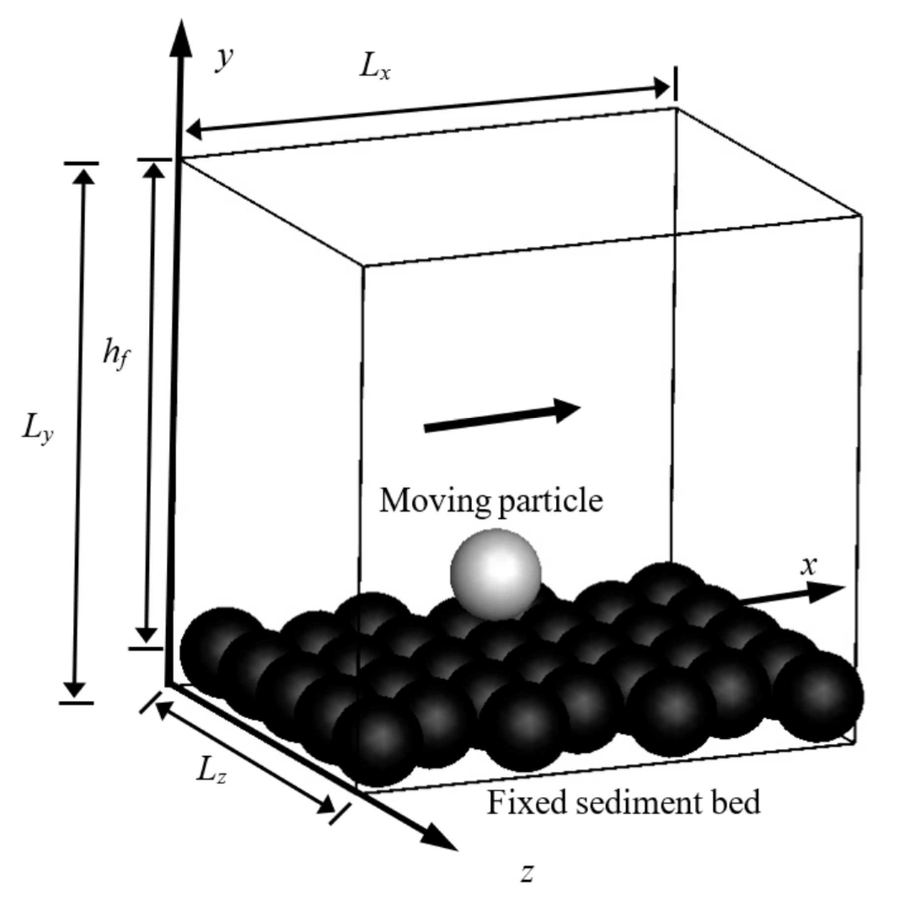
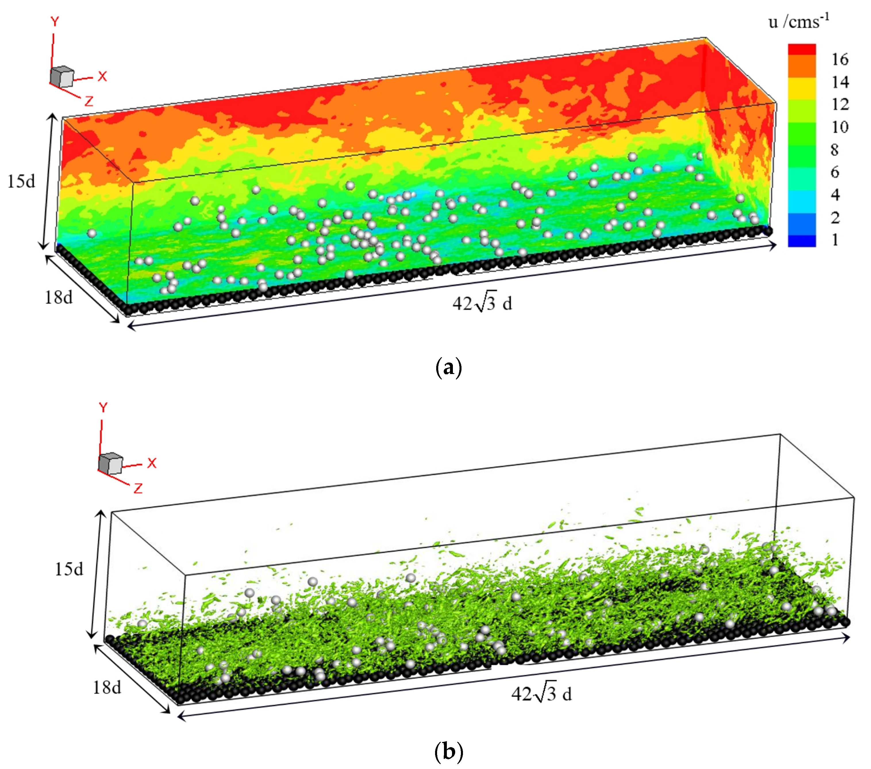
3.1. Setup of Numerical Model

The numerical simulation of sediment particle movement on plane sediment bed in the present study was carried out in a three-dimensional (3D) domain, with the Cartesian coordinates x, y, and z aligned in the streamwise, vertical (upward positive), and spanwise directions, respectively (Figure 1). In order to investigate the different modes of sediment particle movement on the rough bed, a layer of sediment particle was fixed and arranged in a hexagonal lattice in the bottom of the computational domain. The no-slip boundary condition was applied to the bottom of the computational domain; a free-slip rigid lid boundary condition was applied to the top of the fluid domain; and periodic boundary conditions were imposed in the upstream, downstream, and cross-stream sides of the computational domain. Considering the large amount of computation costs, and the periodic boundary conditions of the streamwise and lateral side in the model, the streamwise, vertical, and spanwise length of the computational domain were set as $42\sqrt{3}$ d, 15 d, and 18 d, respectively. The setup of the numerical model was based on the setup of other similar numerical models, which is that the width of the computational domain is slightly larger than the height [53].

3.2. Sediment Transport and Hydraulic Parameters of Numerical Model

The motion characteristics of the sediment particle transport depend on a variety of parameters, such as the density and shape of the moving particles, solid volume fraction, Shields number, particle Reynolds number, Galileo number, and bed structure [14,53,54]. In this study, the sediment particles were assumed to be the “smooth” sphere with a diameter of d = 1 mm; the density was 2.650 g/cm³. The net water depth $h_f$ was 14.25 d. There were 100 particles in the computational domain for statistical convenience, and the global solid volume fraction was set to ${\varphi }_s=8\times {10}^{-5}$. The important parameters were calculated as follows: the friction velocity was calculated as $u_{\ast }=\sqrt{\tau /{\rho }_f}$, where $\tau$ is the shear stress estimated using a linear extrapolation of the total shear stress profile to the rough channel bed [45]. The Shields number was defined as $\theta =\tau /(({\rho }_s-{\rho }_f)gd)$; the bulk velocity $u_b={\displaystyle {\int }_{y_b}^h{u}_{f}dy/h_f}$; the Reynolds number based on bulk flow velocity ${\mathrm{Re}}_b=u_b{h}_f/\nu$; and the Reynolds number based on friction velocity ${\mathrm{Re}}_{\tau }=u_{\ast }{h}_f/\nu$, where $\nu$ is the fluid kinematic viscosity. The particle Reynolds number was calculated as ${\mathrm{Re}}_p=u_{\ast }d/\nu$. The Galileo number was defined as $Ga=\sqrt{\left({\rho }_s/{\rho }_f-1\right)g{d}^3/{\nu }^2}$. The computational domain was discretized by a uniform isotropic grid with grid spacing in terms of wall units $\Delta x^{+}=\Delta y^{+}=\Delta z^{+}=\Delta x\rho u_{\ast }/\nu$.

Table 1. Physical and numerical parameters of numerical model.

Parameter	Value	Parameter	Value
$u_b$$/u_{\ast }$	9.17	$\left(L_x\times L_y\times L_z\right)/d$	$42\sqrt{3}\times 18\times 15$
$\theta$	0.12	$d/\Delta x$	16
$R{e}_b$		$N_x\times N_y\times N_z$	$1152\times 288\times 240$
$R{e}_{\tau }$	1671	$\Delta x^{+}\times \Delta y^{+}\times \Delta z^{+}$	$6.25\times 6.25\times 6.25$
$R{e}_p$	118	${\eta }^{+}$	3.5
$Ga$	1270	${\rho }_s/{\rho }_f$	2.65

summarizes the important physical and numerical parameter values adopted in this study.

3.3. Computational Procedure of Numerical Model

The computational procedure of the simulated cases involved two stages. In the first stage, the sediment particles were fixed at their positions, and the streamwise gravity component g_x was imposed on the fluid to generate fully developed turbulence in the computational domain. In the second stage, the sediment particles were released to move under the hydrodynamic forces. The motion trajectories and the hydrodynamic forces exerted on particles were tracked at the different flow intensities.

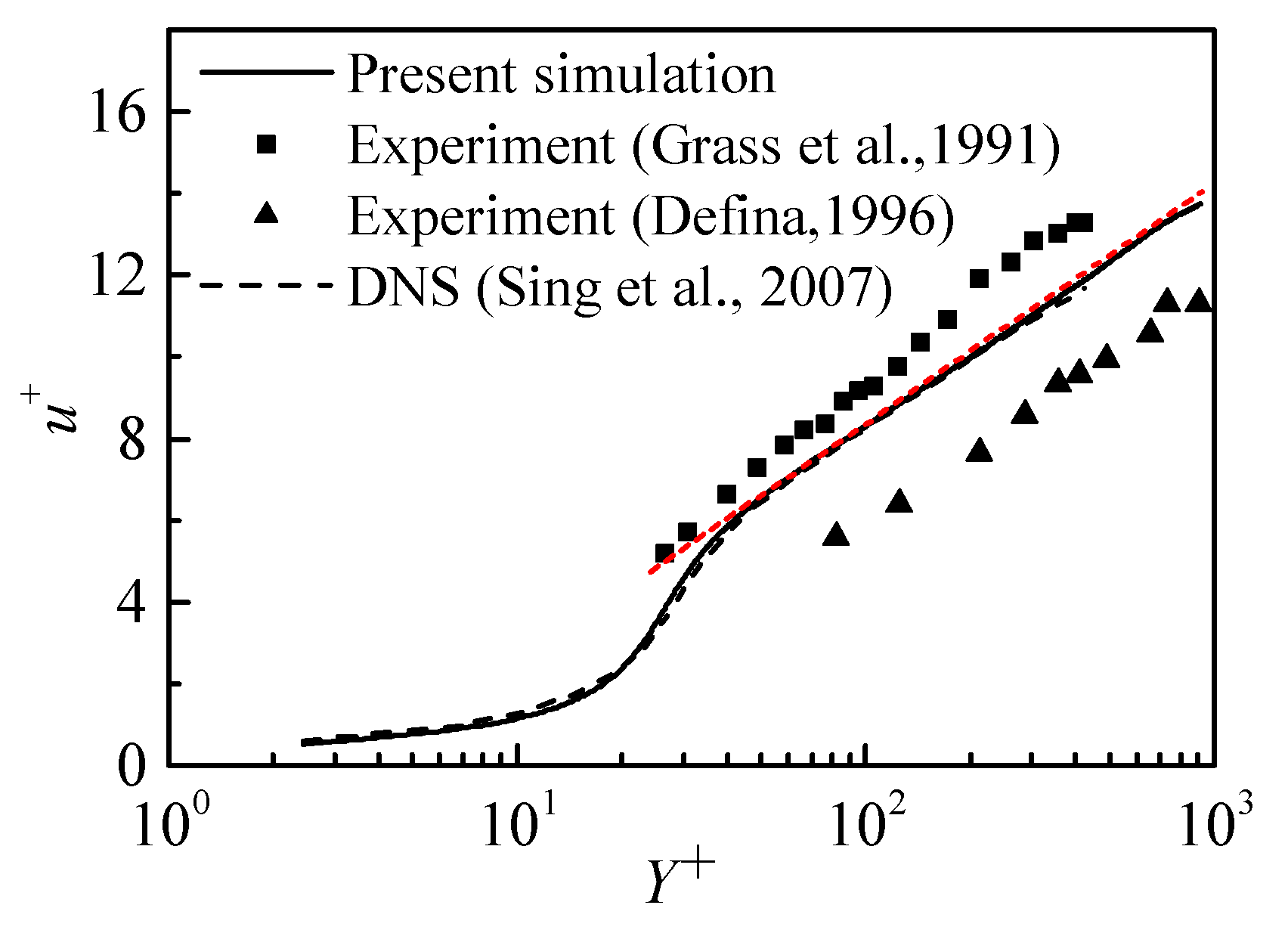
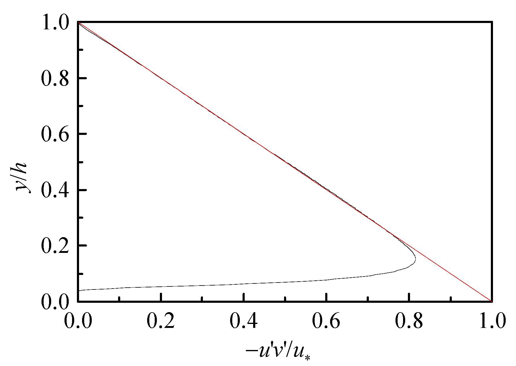
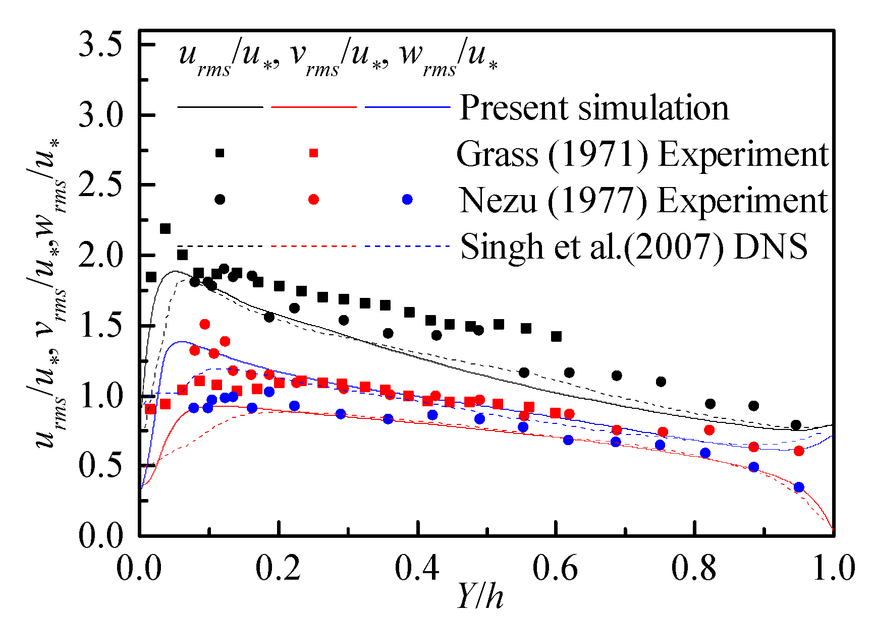
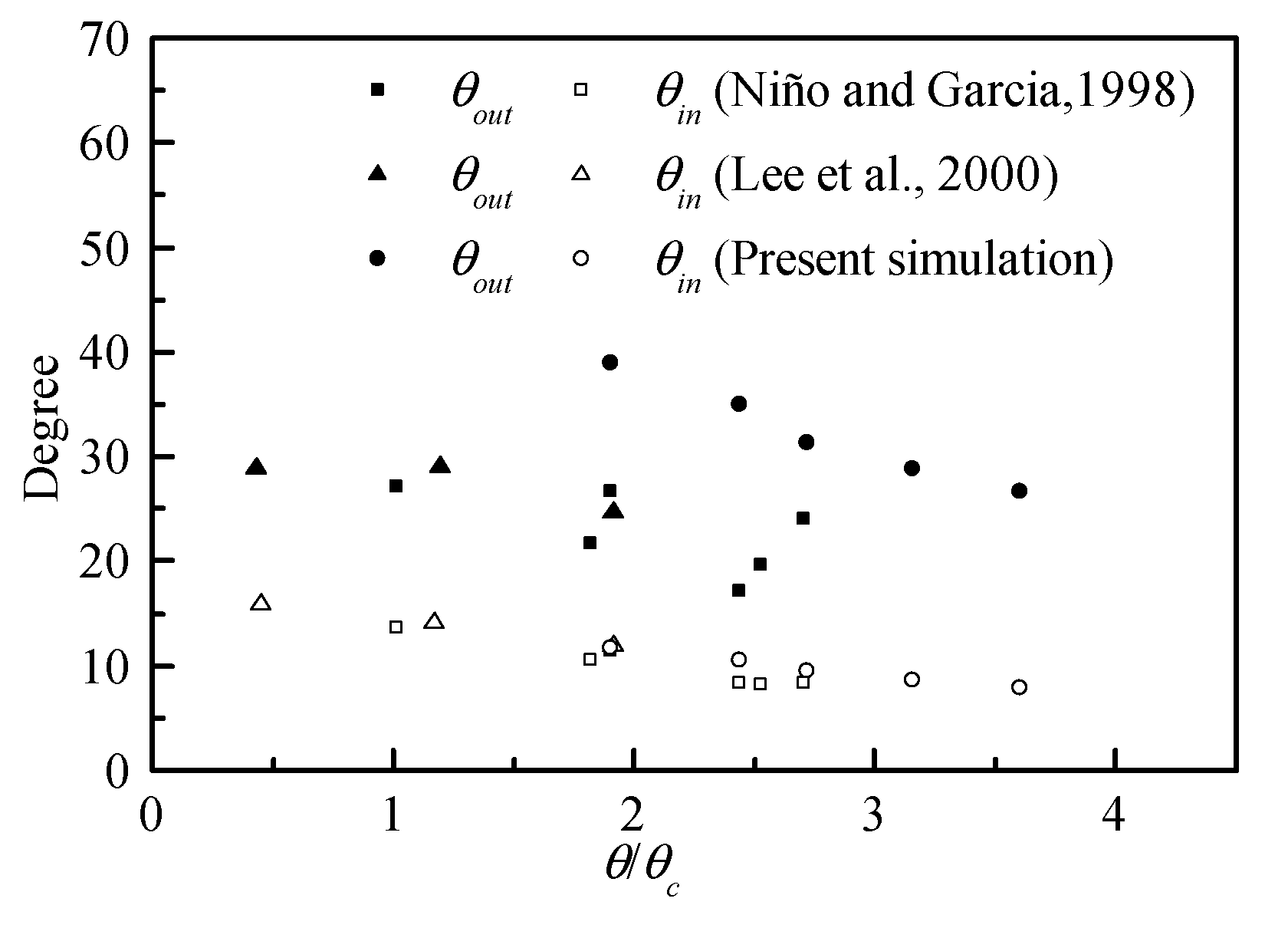
3.4. Validation of Numerical Models

The mean streamwise velocity profile normalized with the bed shear velocity $u_{\ast }$ is presented in Figure 2. $Y^{+}$ is the normalized effective height $(y-y_b)u_{\ast }/\nu$, $y_b$ is the effective location of the bed, which is normally estimated by fitting the mean velocity curve to the logarithmic law-of-the-wall region. Grass et al. [55], Defina [56], and Singh et al. [45] determined equivalent sand roughness k_s = 79.2, 288, and 102 by fitting mean velocity profiles to the logarithmic law-of-the-wall. Using a similar approach, equivalent sand roughness k_s was equal to 110 in the present study. Through a comparison with the experimental results of Defina [56] and Grass et al. [57], it is indicated that the flow profile followed the standard pattern of velocity defect increasing with wall roughness.

The Reynolds shear stress normalized by the bed shear stress is shown in Figure 3, together with the total shear stress on the smooth bed. The profile of the Reynolds shear stress presented a straight line away from the bed and no significant deviations compared with the total shear stress profile for the smooth. It is indicated that the turbulent flow was indeed fully developed on the rough particle bed.

The turbulence intensities normalized by the bed shear velocity are shown in Figure 4, together with the experimental results from Grass [57] and Nezu [58], and the numerical simulation results from Singh et al. [45]. The simulated turbulence intensities in three directions are also in good agreement with both experimental and DNS data.

4. Results and Discussion of Sediment Particle Movement

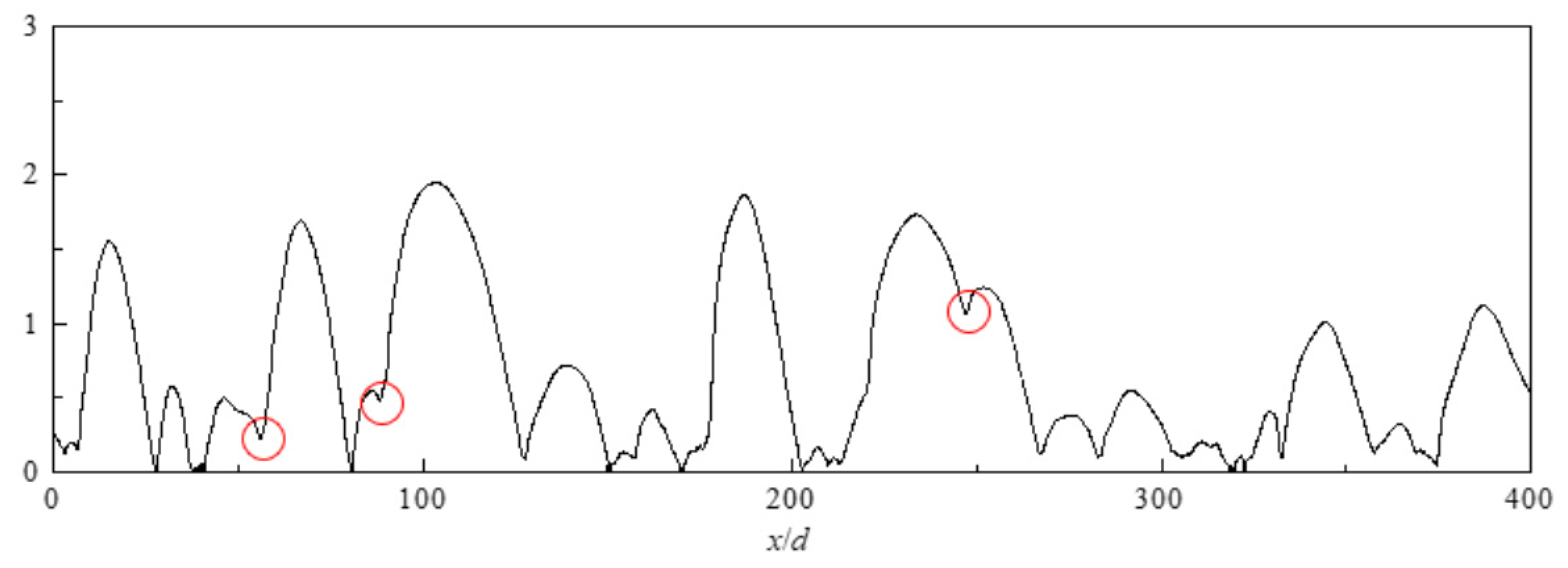
4.1. Processes of Sediment Particle Movement

The sediment particle movement near the bed under a turbulent flow is an inherently complex problem. In this study, the high-precision numerical models were used to investigate the dynamic behaviors and the corresponding hydrodynamic forces (they are derived from the average value of the surface points on the sediment particle) of sliding or rolling and saltation sediment particles. Figure 5 shows the model results of the instantaneous contours of the streamwise velocity, the Q-criterion eddy iso-surface of coherent structures, and the particles distribution. It is indicated that the sediment particles close to the bed are induced to move under the velocity fluctuation of high and low strip and coherent structures.

Figure 6 presents the typical continuous trajectories and dynamic behaviors of individual particle movement and the corresponding hydrodynamic forces exerted on sediment particles with a resolution of 0.00005 s. From the trajectory variations of sediment particle movement, it clearly indicates that a sediment particle moves forward in the mode of sliding or rolling and saltation; the different motion modes are intermittent with time. From the variation of the dynamic responses of sediment particle movement, it indicates that the streamwise and vertical velocity of the particle are disturbed under the instantaneous impulses of hydrodynamic forces during coherent structures. From the variations of the hydrodynamic forces exerted on sediment particles, it shows that the hydrodynamic forces of the moving particle present relatively obvious changes during the process of the moving particle’s contact with the bed. At the moment of sediment particle saltation, the absolute value of the drag force increases drastically then decreases gradually. The lift force plays a more important role than the drag force in the saltation process. Particle rotation is mainly controlled by the particle’s collisions with the bed. From the variation of the particle’s angular velocity (the clockwise rotation along the z direction is positive), when the particle collides with the fixed particle, the particle’s takeoff angular velocity is obviously larger than the particle’s incidence angular velocity, and the particle’s angular velocity increases drastically and reaches the maximum value, then decreases gradually owing to the viscous effects.

Bed loads move randomly and intermittently in sliding or rolling and saltation modes under the turbulence flow. Böhm et al. [59] and Frey [60] studied the bed load motion modes on the rough bed with three particle layers on average by experiment and distinguished the rolling and saltation of the sediment particle based on the threshold velocity (u₀) and distance (d_n is the measured distance between the mass centers from the particle to the next neighbor particle based on averaged five consecutive frames). The parameter values of the threshold velocity (u₀= 0.025 m/s) and distance (d_n/d < ε, ε < 1.07) between the particles were determined by trial and error to minimize the differences between the different motion state. Auel et al. [61] investigated the isolate sediment transport modes on the fixed bed and differentiated the sediment particle rolling and saltation according to threshold height (if particle center exceeded a threshold distance (0.6 d) away from the bed surface, the particle was assumed to change its mode from rolling to saltation). Based on the studies [59,60,61], the threshold height and distance (Figure 7) are adopted to distinguish the sediment particle motion modes in this study. The two threshold parameters are determined compared with the trajectories and hydrodynamic forces of sediment particle movement (Figure 6). If the vertical distance d_v between moving particles and fixed particles is less than 1.1 d (corresponding threshold distance (0.6 d) of Auel et al., 2017 [61]), and the horizontal distance d_l between the same particle’s continuous contact with fixed particles is less than 1.74 d, then the sediment particle is assumed to be a rolling or sliding particle (SRP). If the vertical distance d_v between moving particle and fixed particle is larger than 1.1 d, the sediment particle is assumed to be a saltation particle (SP). The distribution of statistical characteristics of different motion modes of sediment particles are investigated based on the simulated results, including the velocity and angle velocity, the saltation height and length, and the incidence angles and takeoff angles of sediment particles.

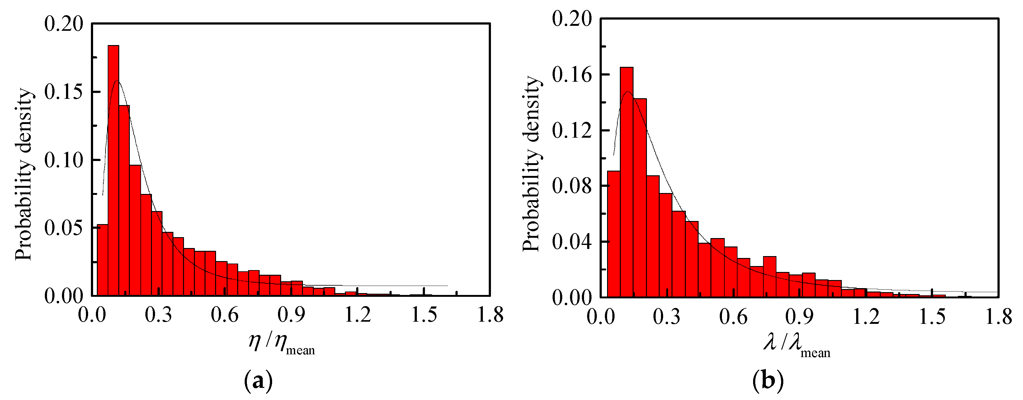
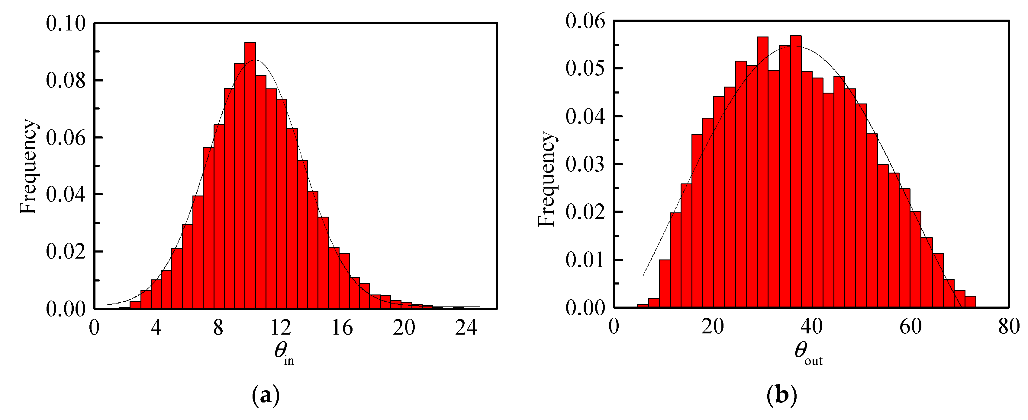
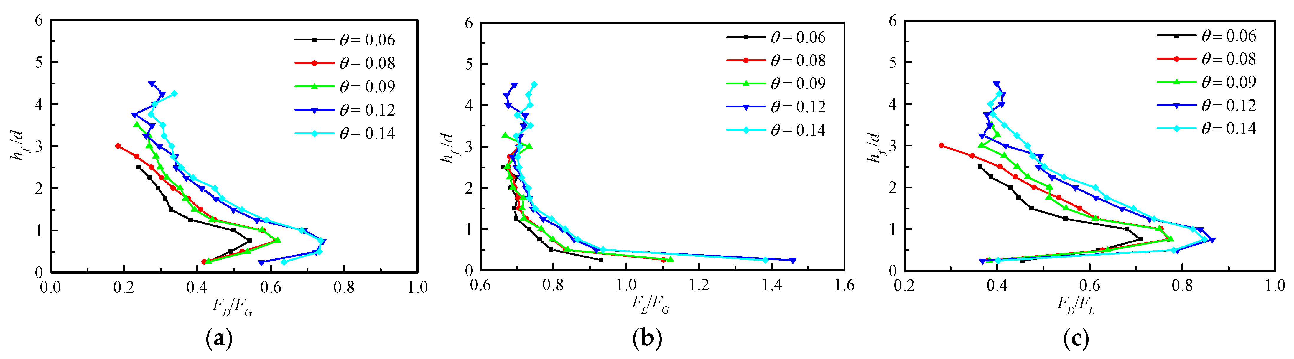
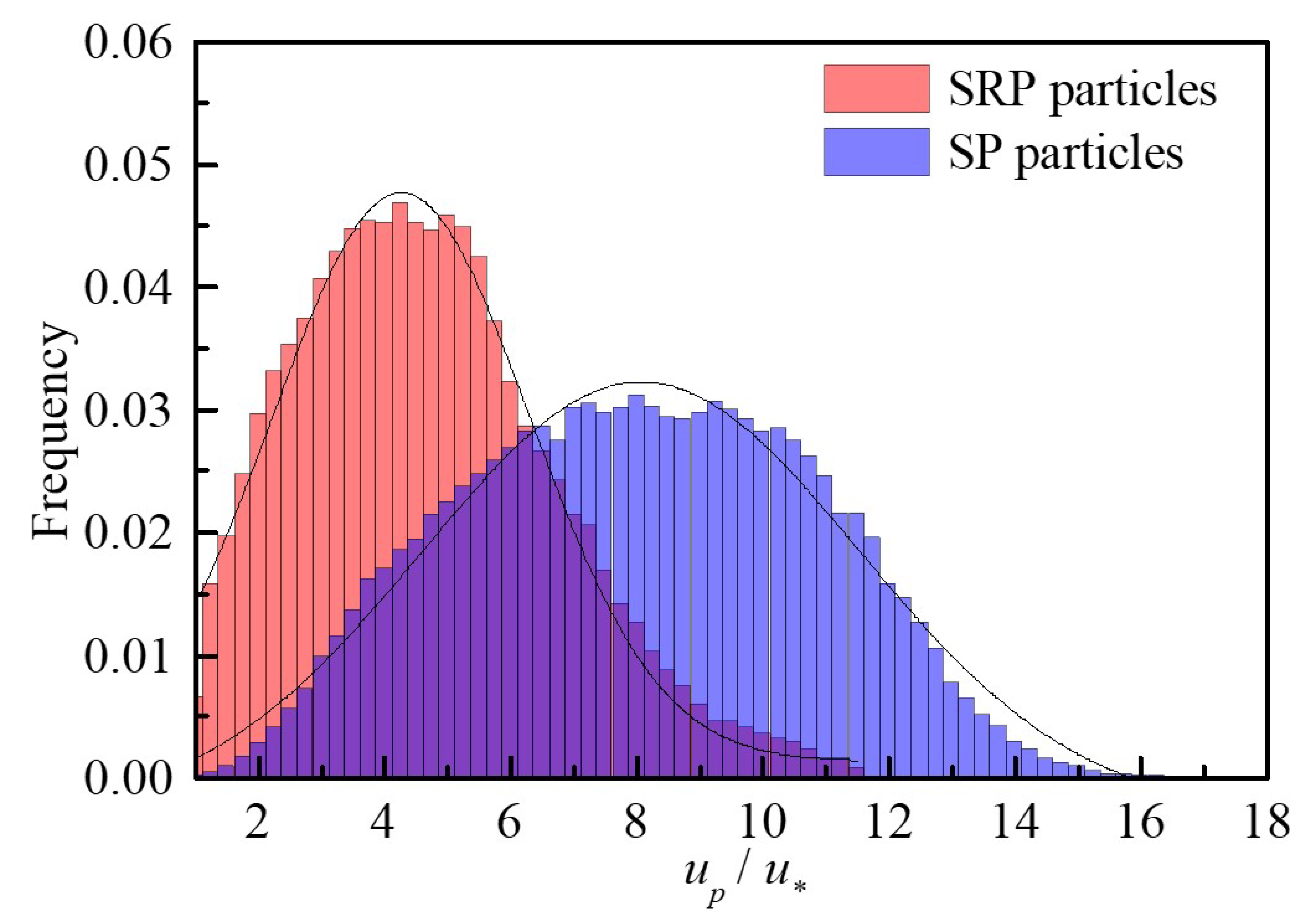
4.2. Results of Saltation Sediment Particle Movement

The predicted results of the empirical formula for the height, length, and velocity of the saltation sediment proposed by some researchers based on the experimental data are quite scattered [14,62]. The reasons may be the sediment shape, size and density, the bed roughness, and the flow intensity. The other reason may have resulted from the different modes of sediment particle movement. The model results under the six different flow intensities are analyzed to investigate the statistical characteristics of sediment particle movement, including the saltation height and length, movement velocity, the incidence, and takeoff angles. In order to make a better comparison between the present simulated results and experimental results, some experimental data for the saltation characteristics of the sediment particle were obtained from the previous study. A brief description of the configuration and parameters of these experiments is presented in

Table 2. Configuration and parameters of experiments by different investigators.

Researcher	u* (m/s)	h (m)	Diameter (mm)	hf/d	Density (g/cm3)	Bed Type	Materials	Number
Lee and Hsu (1994) [8]	0.04–0.11	0.04–0.12	1.36,2.47	26–88	2.640	Fixed	sand	Isolate
Niño and García (1994) [12]	0.14–0.23	0.07–0.15	15,31	2.6–4	2.650	Movable	sand	A little
Niño and García (1998) [9]	0.02–0.05	0.04–0.12	0.5	53–96	2.650	Fixed	sand	A little
Lee et al. (2000) [18]	0.03–0.05	0.05	6	8.3	2.080–2.380	Fixed	sand	Isolate

.

In this study, the saltation height and length, and incidence and takeoff angle of the saltation sediment are studied and compared with the experimental results. Figure 8 shows the probability density distributions of dimensionless saltation length and height for SP. It is indicated that the dimensionless saltation length and height both follow the Γ function distribution, which is similar to the distribution pattern of the experimental results [15]. The distribution pattern is mainly related to the velocity fluctuations of the flow and the bed roughness. Lu and Willmarth [63] pointed out sediment particle saltation mainly occurs during sweeps (fourth quadrant) and outward interactions (first quadrant), while saltation is almost negligible during ejections (second quadrant) and inward interactions (third quadrant) in the quadrant events under the action of turbulent structures. Furthermore, the collisions between saltation particles increase the saltation length and height, as can be seen in Figure 9. Similarly, the collisions between saltation particles increase the probability of a larger flight time and cause the flight time following the logarithmic normal distribution, as can be seen in Figure 10.

A comparison of the dimensionless saltation length between the present simulated results and experimental results is plotted in Figure 11. It indicates that dimensionless saltation length increases as the transport stage increases. At the lower transport stage, the simulated results of dimensionless saltation length are very close to the experimental results [9,17], which verify the correctness of the numerical model. At the medium transport stage, the simulated results are larger than the experimental results. Einstein and El-Sammi [64] pointed out that saltation length is affected by particle size and shape; their opinions are verified by the experiment of Lee et al. [18] at the low flow intensity, in which they pointed out that at the low flow intensity, the dimensionless saltation length and height increase with the particle diameter. Amir et al. [65] believed that the maximum saltation height increases with the increase of the flow depth and particle density. At the medium transport stage, the simulated results are larger than the experimental results. The reason may be that the moving sediment particles collide with each other under the turbulent flow structure, and the inter-particle collisions increase the saltation length, as can be seen in Figure 9. Lee et al. [66] investigated the inter-particle collision behaviors during the saltating process of multiple particles, and found that the maximum saltation height was about 2–2.5 times the values calculated by a single-particle saltation. It is also verified that the trajectories of saltation particles due to inter-particle collision has multiple peak positions, which are clearly different from the typical trajectory of single-particle saltation.

Figure 12 presents a comparison of the dimensionless saltation height between the present simulated results and the experimental results. It is found that the dimensionless saltation height increases with the increase of the transport stage. At the low transport stage, the dimensionless saltation height is in good agreement with the experimental results by Niño and García [9,17]. Similar to the saltation length, the difference of saltation height between the present simulated results and experimental results at the medium transport stage may be induced by the inter-particle collision, particle size, and flow depth. Moreover, Auel et al. [61] indicated that for a given transport stage, the saltation height for a mild bed slope is larger than that for a steep slope, and the differences reduce with the increase of the transport stage.

The sediment particles under the action of turbulent flow collide with the bed, and three important collision angles are used to characterize the saltation process, i.e., incidence angle ${\theta }_{in}$, takeoff angle ${\theta }_{out}$, and collision position angle ${\theta }_b$ as shown in Figure 13. The angles of incidence ${\theta }_{in}$ and takeoff ${\theta }_{out}$ are defined with respect to a line parallel to the channel bottom, and they are calculated through the particle trajectory right before and after the collision [33]. The collision position angle ${\theta }_b$ is the angle between the tangential collision surface and the bed bottom. Based on the magnitude of the collision position angle, the collision point is located on the upstream (${\theta }_b$ > 0) and downstream faces (${\theta }_b$ < 0) of the bed particle. In this study, the analysis on the incidence angle ${\theta }_{in}$ and takeoff angle ${\theta }_{out}$ are presented. The results on the collision position angle ${\theta }_b$ involve the analysis of the “splash function”, which will be studied in future research work.

Figure 14 shows the frequency of distributions of the incidence angle ${\theta }_{in}$ and takeoff angle ${\theta }_{out}$; the distribution is also similar to the experimental results [18]. The distributions of the incidence and takeoff angles can be approximately described using the skew-normal distribution function. The distribution pattern is closely related to the random collision of sediment particle-bed and the flow turbulent fluctuations. Bhattacharyya et al. [67] pointed out that the shape of the normal distribution depends on the particle size and bed roughness. In general, the particle’s takeoff angle at collision is larger than the particle’s incidence angle. This observation is largely supported by the experimental data [12,18,61]. This phenomenon is related to the asymmetry of the forces exerted on the sediment particles. The saltation process of sediment particles is due to the combined interaction of lift and drag forces and the submerged weight. In the rising phase of the SP trajectory, the hydrodynamic lift $F_L$ and the submerged weight G of the sediment particle are directed downwards; in the recession phase, the hydrodynamic drag $F_L$ is directed upwards and opposes the submerged weight G.

The particle’s incidence angles θ_in and takeoff angles θ_out change due to the combined interaction of lift and drag forces and the submerged weight under different flow intensities. Figure 15 presents the variation of incidence angles and takeoff angles with the transport stage. It indicates that the incidence and takeoff angles decrease with the increase of flow intensity. This is related to the relative magnitude of the drag and lift forces (Figure 16c). It also indicates that the present simulated results of incidence angles agree with the experimental results, but the takeoff angles are larger than the experimental results [9,18]. The reason may be related to the arrangement of bed and water depth.

The drag and lift forces play significant roles in the sediment movement, and influence the motion modes of sliding or rolling, saltation, and suspension. Figure 16 presents the variation and relative magnitude of the dimensionless drag and lift forces in the vertical direction above the bed. It indicates that the drag forces are large near the sediment bed and increase with the increase of the flow intensity, while the lift forces do not change significantly along the flow depth. From the relative magnitude of the drag and lift forces, the lift force plays a more important role than the drag force in the sediment saltation [18].

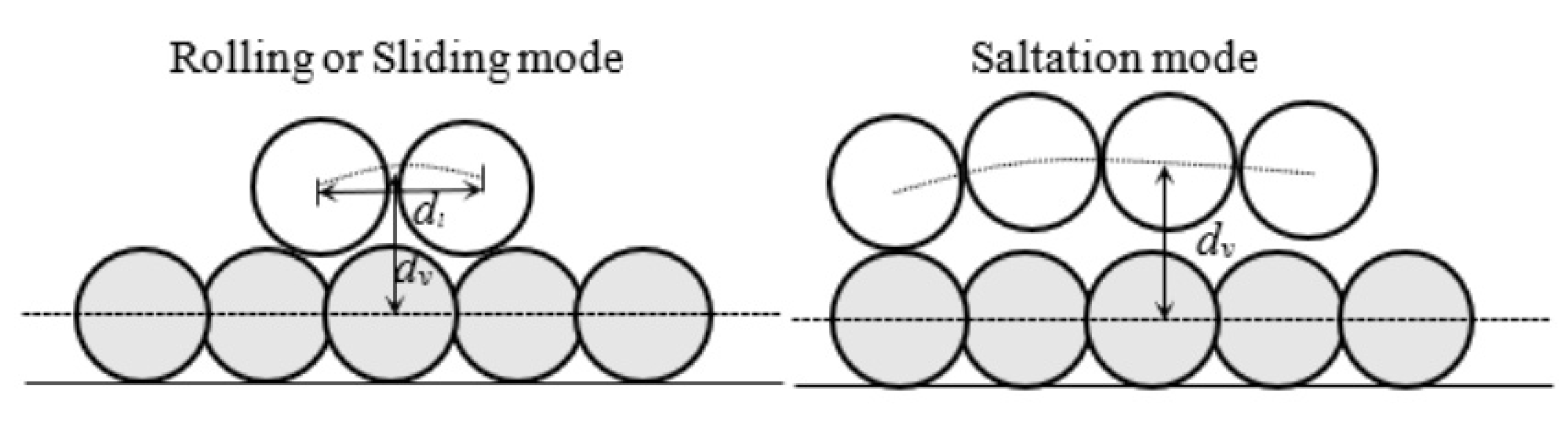
4.3. Discussion of Sliding or Rolling and Saltation Sediment Particle Movement

Previous studies mainly focused on the sediment saltation (Shim and Duan, 2017 [15]); therefore, the motion characteristics of different movement modes of bed load particles are investigated in this study.

Figure 17 presents the frequency distributions of the dimensionless velocity of SRP and SP. Through curve fitting of the streamwise velocity distributions of sediment particles, skew-normal distributions are found for SRP and SP, respectively, which are similar to the distribution patterns of the experimental results [18] and simulated results [33]. The reason for this skew-normal distribution is related to the disturbance of flow velocity near the bed. The fluid resistance in the flow direction and bed friction resistance induced the asymmetric of particle velocity distribution. The difference between two frequency distributions of the dimensionless velocity is that the mean value of the skew-normal distribution of the SRP is smaller than that of the SP. This is related to the fact that the saltating particles achieved higher and longer trajectories, which induced in the SP obtained more speed and energy from the flow than the SRP. Furthermore, bed resistance has greater influence on the SRP than the SP.

The formulas of mean velocity of a saltating particle are proposed by the different investigators based on experimental data, as can be seen in

Table 3. Formulas of mean velocity ${\overline{u}}_b$ of saltating particles given by different investigators.

Investigators	Mean Velocity of Particle	Material	Diameter(mm)
Engelund and Fredsøe (1976) [11]	${\overline{u}}_b=u_{\ast }\left(10-0.7{\left(\theta -{\theta }_c\right)}^{0.5}\right)$	Sand	-
Van Rijn (1985) [7]	${\overline{u}}_b/u_{\ast }=9+2.6\log D_{\ast }-8{\left({\theta }_c/\theta \right)}^{0.5}$	Gravel	1.8
Lee and Hsu (1994) [8]	${\overline{u}}_b=11.53{\left(\theta -{\theta }_c\right)}^{0.174}$	Sand	1.36, 2.47
Hu and Hui (1996) [13]	${\overline{u}}_b=11.9{\left(u_{\ast }-0.44u_{\ast c}\right)}^{0.174}$	Gravel	1.34–7.6

. Figure 18 presents a comparison of the dimensionless streamwise saltation velocity between the present simulated results and the empirical formula [7,8,11,13]. It is found that the predicted results of the empirical formula are quite scattered, except for the empirical formula [7,8]. In this study, the present simulated results of the SRP and SP are presented in order to analyze the distinction of different movement modes. Figure 18 indicates that the present simulated results of the SRP are lower than the predicted results of the empirical formula, and the present simulated results of the SP are between the curves of the empirical formula. For the SRP, the sediment particles move near the sediment bed and contact with the bed frequently, so the bed resistance decreases the streamwise velocity of the SRP. For the SP, the collisions between sediment particles under the strong turbulence structure increase the flight time, and cause saltation particles to absorb more energy from the flow and increase sediment particle velocity. The other possible reason for the difference between the present simulated results and the predicted results of the empirical formula is the shape and size of particles. The smooth particles move with the lower and shorter jumps more than the rough particles of the same mean diameter, and are less influenced by the flow velocity than the coarse particles; therefore, the velocities of smooth particles are less than those of the rough particles [68].

It is well known that the sediment particles move in both translational and rotational motion, and the rotation of sediment particles has a significant effect on their trajectories [8,9,25]. Sediment particle rotation occurs under the combined effects of the bed roughness, particle-bed collision, and the velocity gradient of the carrier fluid. In the previous experiment, the particle’s angular velocity was hard to describe exactly due to the limits of the measurement technique. The dimensionless angular velocity of particle $\Omega$ is defined as

$$\Omega =sd/u_{\ast }$$

(13)

The frequency distributions of the instantaneous dimensionless angular velocity of the SRP and SP around z direction at the different vertical positions is presented in Figure 19. Through curve fitting of the frequency distributions of instantaneous dimensionless angular velocity, it shows that, for the SRP, the frequency distribution of dimensionless angular velocity follows skew-normal distribution, while for the SP, the frequency distribution of dimensionless angular velocity follows a logarithmic normal distribution. The different distribution patterns are mainly related to the motion modes of the sediment particle. Particle rotation is mainly derived from sediment particle-bed collisions. The SRP slide and roll close to the bed and frequently contact with the bed, while the SP are intermittently losing contact with the bed for a short time and are strongly influenced by the fluid velocity near the bed.

Figure 20 presents the variation of particle angular velocity with the transport stage. It indicates that the angular velocity of the SP decreases with the increase of the transport stage; this trend is similar to the experimental results of Niño and García [9]. The difference may result from the particle shape and bed roughness. The shape of the particle affects the angular velocity of the particle, because a particle with an elongated shape colliding with the bed results in a higher angular velocity than a spherical shape [68]. Niño and García [9] pointed out that the particle angular velocity is controlled mainly by the process of collision with the bed. This phenomenon can be seen in Figure 7. The incidence angle and takeoff angle at collision also influence the particle angular velocity [8]. It also indicates that the angular velocity of the SRP increases with the increase of the transport stage. The greater the transport stage, the faster the rolling sediment particles move, and accordingly, the greater the angular velocity of the SRP.

5. Conclusions

In this study, the motion trajectories, the dynamic responses, the corresponding hydrodynamic forces, and the statistical characteristics of sediment particle movement (sliding, rolling, and saltation) are studied through simulating the movement of sediment particles using a coupled CFD-FDEM model. The conclusions are summarized as follows:

The bed load sediment particles have a different motion trajectory under the fluctuating velocity of turbulent flow. The inter-particle collision between moving sediment particles has an important effect on the characteristics of moving sediment particles. The inter-particle collision in the low concentration increases the saltation length, height, and flight time, correspondingly increasing the velocity of the saltating sediment particle. The frequency distribution of dimensionless angular velocity for the sliding and rolling sediment particle follows skew-normal distribution, while for the saltation sediment particle it follows a logarithmic normal distribution. Therefore, the inter-particle collision effect between particles should be considered in the calculation of sediment transport rate.

The collision between moving sediment particles and the bed has an important effect on the motion pattern and characteristics of moving sediment particles. The hydrodynamic forces exerted on a sediment particle away from the bed are smooth, while near the bed they present a relatively obvious disturbance owing to the contact between the sediment particle and the bed. The drag force near the bed is large, and away from the bed it decreases gradually during the whole movement process. The relative magnitudes of drag and lift forces influence the incidence and takeoff angles of saltation sediment particles. The particle’s angular velocity is the largest at the takeoff moment, then decreases gradually owing to the viscous effects. The research results are helpful to further understand the distinction of motion characteristics of sliding, rolling, and saltating sediment particles, and to better predict the bed load transport rates.

References

1. Einstein, H.A. The bed-load function for sediment transport in open channel flows. Tech. Bull. 1950, 1026, 1–71. [Google Scholar]
2. Bagnold, R.A. An approach to the sediment transport problem from general physics. In Geological Survey Professional Paper 422-I; Government Printing Office: Washington, DC, USA, 1967. [Google Scholar]
3. Gordon, R.; Carmichael, J.B.; Isackson, F.J. Saltation of plastic balls in a one-dimensional flume. Water Resour. Res. 1972, 8, 444–459. [Google Scholar] [CrossRef]
4. Francis, J.R.D. Experiments on the motion of solitary gains along the bed of a water stream. Philos. Trans. R. Soc. 1973, 332, 443–471. [Google Scholar]
5. Abbott, J.E.; Francis, J.R.D. Saltation and suspension trajectories of solid grains in a water stream. Philos. Trans. R. Soc. A 1977, 284, 225–254. [Google Scholar]
6. Murphy, P.J.; Hooshiari, H. Saltation in water dynamics. J. Hydraul. Div. 1982, 108, 1251–1267. [Google Scholar] [CrossRef]
7. Van Rijn, L.C. Sediment transport, Part I: Bed load transport. J. Hydraul. Eng. 1985, 110, 1431–1456. [Google Scholar] [CrossRef] [Green Version]
8. Lee, H.Y.; Hsu, I.S. Investigating of saltating particle motions. J. Hydraul. Eng. 1994, 120, 831–845. [Google Scholar] [CrossRef]
9. Niño, Y.; García, M. Experiments on saltation of sand in water. J. Hydraul. Eng. 1998, 124, 1014–1025. [Google Scholar] [CrossRef]
10. Fernandez, L.R.; Van Beek, R. Erosion and transport of bed sediment. J. Hydraul. Res. 1974, 14, 127–144. [Google Scholar] [CrossRef] [Green Version]
11. Engelund, F.; Fredsøe, J. A sediment transport model for straight alluvial channels. Hydrol. Res. 1976, 7, 293–306. [Google Scholar] [CrossRef] [Green Version]
12. Niño, Y.; García, M.; Ayala, L. Gravel saltation. 1. Experiments. Water Resour. Res. 1994, 30, 1907–1914. [Google Scholar] [CrossRef]
13. Hu, C.H.; Hui, Y.J. Bed-load transport. I: Mechanical characteristics. J. Hydraul. Eng. 1996, 122, 245–254. [Google Scholar] [CrossRef]
14. Lajeunesse, E.; Malverti, L.; Charru, F. Bed load transport in turbulent flow at the grain scale: Experiments and modeling. J. Geophys. Res. 2010, 115, F04001. [Google Scholar] [CrossRef]
15. Shim, J.; Duan, J.G. Experimental study of bed-load transport using particle motion tracking. Int. J. Sediment Res. 2017, 32, 73–81. [Google Scholar] [CrossRef]
16. Wiberg, P.L.; Smith, J.D. A theoretical model for saltating grains in water. J. Geophys. Res. 1985, 90, 7341–7354. [Google Scholar] [CrossRef]
17. Niño, Y.; García, M. Gravel saltation. 2. Modeling. Water Resour. Res. 1994, 30, 1915–1924. [Google Scholar] [CrossRef]
18. Lee, H.Y.; Chen, Y.H.; You, J.Y.; Lin, Y.T. Investigations of continuous bed load saltating process. J. Hydraul. Eng. 2000, 126, 691–700. [Google Scholar] [CrossRef]
19. Ballio, F.; Pokrajac, D.; Radice, A.; Sadabadi, S. Lagrangian and eulerian description of bed load transport. J. Geophys. Res. Earth Surf. 2018, 123, 384–408. [Google Scholar] [CrossRef]
20. Anderson, R.S.; Haff, P.K. Simulation of eolian saltation. Science 1988, 241, 820–823. [Google Scholar] [CrossRef]
21. Wiberg, P.L.; Smith, J.D. Calculation of the critical shear stress for motion of uniform and heterogeneous sediments. Water Resour. Res. 1987, 23, 1471–1480. [Google Scholar] [CrossRef]
22. Wiberg, P.L.; Smith, J.D. Model for calculating bed load transport of sediment. J. Hydraul. Eng. 1989, 115, 101–123. [Google Scholar] [CrossRef]
23. Kharlamova, I.S.; Vlasák, P. Model of rough bed for numerical simulation of saltation. Eur. J. Environ. Civ. Eng. 2015, 19, 366–385. [Google Scholar] [CrossRef]
24. Robinson, S.K. Coherent motions in the turbulent boundary layer. Annu. Rev. Fluid Mech. 1991, 23, 601–639. [Google Scholar] [CrossRef]
25. White, B.R.; Schultz, J.C. Magnus effect in saltation. J. Fluid Mech. 1977, 81, 497–512. [Google Scholar] [CrossRef]
26. Cundall, P.A.; Strack, O.D.L. A discrete numerical model for granular assemblies. Géotechnique 1979, 29, 47–65. [Google Scholar] [CrossRef]
27. Thornton, C.; Yin, K.K. Impact of elastic spheres with and without adhesion. Powder Technol. 1991, 65, 153–166. [Google Scholar] [CrossRef]
28. Zhu, H.P.; Zhou, Z.Y.; Yang, R.Y.; Yu, B.A. Discrete particle simulation of particulate systems: Theoretical developments. Chem. Eng. Sci. 2007, 62, 3378–3396. [Google Scholar] [CrossRef]
29. Schmeeckle, M.W. Numerical simulation of turbulence and sediment transport of medium sand. J. Geophy. Res. 2014, 119, 1240–1262. [Google Scholar] [CrossRef]
30. Kidanemariam, A.G.; Uhlmann, M. Interface-resolved direct numerical simulation of the erosion of a sediment bed sheared by laminar channel flow. Int. J. Multiph. Flow. 2014, 67, 174–188. [Google Scholar] [CrossRef] [Green Version]
31. Sun, R.; Xiao, H. SediFoam: A general-purpose, open-source CFD–DEM solver for particle-laden flow with emphasis on sediment transport. Comput. Geosci. 2016, 89, 207–219. [Google Scholar] [CrossRef] [Green Version]
32. Esteghamatian, A.; Hammouti, A.; Lance, M.; Wachs, A. Particle resolved simulations of liquid/solid and gas/solid fluidized beds. Phys. Fluids 2017, 29, 033302. [Google Scholar] [CrossRef]
33. Liu, D.T.; Liu, X.F.; Fu, X.D. LES-DEM simulations of sediment saltation in a rough-wall turbulent boundary layer. J. Hydraul. Res. 2019, 57, 786–797. [Google Scholar] [CrossRef]
34. Zhang, B.W.; Wu, B.S.; Li, S.W.; Shi, Y. Large eddy simulation of sediment transport in high flow intensity by discrete particle method. J. Hydraul. Res. 2021, 59, 605–620. [Google Scholar] [CrossRef]
35. Kidanemariam, A.G.; Uhlmann, M. Direct numerical simulation of pattern formation in subaqueous sediment. J. Fluid Mech. 2014, 750, R21. [Google Scholar] [CrossRef] [Green Version]
36. Kidanemariam, A.G.; Uhlmann, M. Formation of sediment patterns in channel flow: Minimal unstable systems and their temporal evolution. J. Fluid Mech. 2017, 818, 716–743. [Google Scholar] [CrossRef] [Green Version]
37. Sun, R.; Xiao, H. CFD–DEM simulations of current-induced dune formation and morphological evolution. Adv. Water Resour. 2016, 92, 228–239. [Google Scholar] [CrossRef] [Green Version]
38. Jain, R.; Vowinckel, B.; Fröhlich, J. Spanwise particle clusters in DNS of sediment transport over a regular and an irregular Bed. Flow Turbul. Combust. 2017, 99, 973–990. [Google Scholar] [CrossRef]
39. Zhang, B.W.; Li, S.W.; Ji, C.N. Numerical simulation of ripple evolution under turbulent flow using a coupled LES and DPM model. J. Hydraul. Eng. 2018, 144, 04018067. [Google Scholar] [CrossRef]
40. Munjiza, A. The Combined Finite-Discrete Element Method; Wiley: Hoboken, NJ, USA, 2004. [Google Scholar]
41. Xiang, J.; Munjiza, A.; Latham, J.P.; Guises, R. On the validation of DEM and FEM/DEM models in 2D and 3D. Eng. Comput. 2009, 26, 673–687. [Google Scholar] [CrossRef]
42. Ji, C.; Munjiza, A.; Avital, E.; Ma, J.; Williams, J.J.R. Direct numerical simulation of sediment entrainment in turbulent channel flow. Phys. Fluids 2013, 25, 056601. [Google Scholar] [CrossRef]
43. Ji, C.; Munjiza, A.; Avital, E.; Xu, D.; Williams, J. Saltation of particles in turbulent channel flow. Phys. Rev. E 2014, 89, 052202. [Google Scholar] [CrossRef] [PubMed]
44. Thomas, T.G.; Williams, J.J.R. Development of a parallel code to simulate skewed flow over a bluff body. J. Wind. Eng. Ind. Aerodyn. 1997, 67, 155–167. [Google Scholar] [CrossRef]
45. Singh, K.M.; Sandham, N.D.; Williams, J.J.R. Numerical Simulation of Flow over a Rough Bed. J. Hydraul. Eng. 2007, 133, 386–398. [Google Scholar] [CrossRef] [Green Version]
46. Munjiza, A.; Owen, D.R.J.; Bicanic, N.A. combined finite-discrete element method in transient dynamics of fracturing solids. Eng. Comput. 1995, 12, 145–174. [Google Scholar] [CrossRef]
47. Ji, C.; Munjiza, A.; Williams, J.J.R. A novel iterative direct-forcing immersed boundary method and its finite volume applications. J. Comput. Phys. 2012, 231, 1797–1821. [Google Scholar] [CrossRef]
48. Munjiza, A.; Andrews, K.R.F. Penalty function method for combined finite-discrete element systems comprising large number of separate bodies. Int. J. Numer. Methods Eng. 2000, 49, 1377–1396. [Google Scholar] [CrossRef]
49. Roux, J.-N.; Combe, G. Quasistatic rheology and the origins of strain. Comptes Rendus Phys. 2002, 3, 131–140. [Google Scholar] [CrossRef] [Green Version]
50. Simeonov, J.A.; Calantoni, J. Modeling mechanical contact and lubrication in direct numerical simulations of colliding particles. Int. J. Multiph. Flow. 2012, 46, 38–53. [Google Scholar] [CrossRef]
51. Peskin, C.S. The immersed boundary method. Acta Numer. 2002, 11, 479–518. [Google Scholar] [CrossRef] [Green Version]
52. Uhlmann, M. An immersed boundary method with direct forcing for the simulation of particulate flows. J. Comput. Phys. 2005, 209, 448–476. [Google Scholar] [CrossRef] [Green Version]
53. Yousefi, A.; Costa, P.; Brandt, L. Single sediment dynamics in turbulent flow over a porous bed–insights from interface-resolved simulations. J. Fluid Mech. 2020, 893, A24. [Google Scholar] [CrossRef] [Green Version]
54. Kharlamova, I.S.; Vlasák, P. Dependence of saltation characteristics on bed organisation in numerical simulation. Geosci. J. 2015, 19, 177–184. [Google Scholar] [CrossRef]
55. Grass, A.J.; Stuart, R.J.; Mansour-Tehrani, M. Vortical structures and coherent motion in turbulent flow over smooth and rough boundaries. Philos. Trans. R. Soc. Lond. 1991, 336, 33–65. [Google Scholar]
56. Defina, A. Transverse spacing of low-speed streaks in a channel flow over a rough bed. Coherent Flow Struct. Open Channels 1996, 4, 87–99. [Google Scholar]
57. Grass, A.J. Structural features of turbulent flow over smooth and rough boundaries. J. Fluid Mech. 1971, 50, 233–255. [Google Scholar] [CrossRef]
58. Nezu, I. Turbulence Structure in an Open Channel Flow. Ph.D. Thesis, Kyoto University, Kyoto, Japan, 1977. [Google Scholar]
59. Böhm, T.; Frey, P.; Ducottet, C.; Ancey, C.; Jodeau, M.; Reboud, J.L. Two-dimensional motion of a set of particles in a free surface flow with image processing. Exp. Fluids 2006, 41, 1–11. [Google Scholar] [CrossRef]
60. Frey, P. Particle velocity and concentration profiles in bedload experiments on a steep slope. Earth Surf. Proc. Landf. 2014, 39, 646–655. [Google Scholar] [CrossRef]
61. Auel, C.; Albayrak, I.; Sumi, T.; Boes, R.M. Sediment transport in high-speed flows over a fixed bed: 1. Particle dynamics. Earth Surf. Proc. Landf. 2017, 42, 1365–1383. [Google Scholar] [CrossRef]
62. Maldonado, S.; Borthwick, A.G.L. Sensitivity analysis and statistical convergence of a saltating particle model. J. Hydraul. Eng. 2016, 141, 04014091. [Google Scholar] [CrossRef] [Green Version]
63. Lu, S.S.; Willmarth, W.W. Measurements of the structure of the Reynolds stress in a turbulent boundary layer. J. Fluid Mech. 1973, 60, 481–511. [Google Scholar] [CrossRef]
64. Einstein, H.A.; El-Sammi, E.A. Hydrodynamic forces on a rough wall. Rev. Mod. Phys. 1949, 21, 520–524. [Google Scholar] [CrossRef] [Green Version]
65. Amir, M.; Nikora, V.; Witz, M. A novel experimental technique and its application to study the effects of particle density and flow submergence on bed particle saltation. J. Hydraul. Res. 2017, 55, 101–113. [Google Scholar] [CrossRef] [Green Version]
66. Lee, H.Y.; You, J.Y.; Lin, Y.T. Continuous saltating process of multiple sediment particles. J. Hydraul. Eng. 2002, 128, 443–450. [Google Scholar] [CrossRef] [Green Version]
67. Bhattacharyya, A.; Ojha, S.P.; Mazumder, B.S. Evaluation of the saltation process of bed materials by video imaging under altered bed roughness. Earth Surf. Proc. Landf. 2013, 38, 1339–1353. [Google Scholar] [CrossRef]
68. Vlasak, P.; Kysela, B.; Chara, Z. Flow structure of coarse-grained slurry in a horizontal pipe. J. Hydrol. Hydromech. 2012, 60, 115–124. [Google Scholar] [CrossRef]
Figure 1. Computational domain and coordinate system.
Water 14 01506 g001
Figure 2. Mean velocity profiles. The red short-dashed line indicates the fitted velocity profile according to the logarithmic law-of-the-wall [45,55,56].
Water 14 01506 g002
Figure 3. Reynolds shear stress normalized by the bed shear velocity. The black solid line represents Reynolds shear stress u ' v ' / u 2 on the rough bed; the red solid line represents total shear stress on the smooth bed.
Water 14 01506 g003
Figure 4. Turbulence quantities [45,57,58].
Water 14 01506 g004
Figure 5. Instantaneous velocity and vorticity fields of the flow and particle distribution. The black particles are bed; the gray particles are the moving sediment particles. (a) Instantaneous contours of the streamwise velocity and the particle distribution. (b) Instantaneous vortical structures and the particle distribution. The blue iso-surface indicates the vortical structure, Q = 12,000, which is the second invariant of the velocity gradient tensor.
Water 14 01506 g005
Figure 6. Typical continuous trajectories and dynamic behaviors of individual sediment particle movement (sliding, or rolling and saltation), and the corresponding hydrodynamic forces exerted on the particle. x p and y p = streamwise and vertical center coordinates of the particle, respectively; u p and v p = streamwise and vertical velocities of the particle, respectively; F D and F L = drag and lift forces of hydrodynamic forces exerted on the particle, respectively; s x = angular velocity of the particle; and G = particle submerged weight.
Water 14 01506 g006
Figure 7. Criteria of distinction between sliding, rolling, and saltation.
Water 14 01506 g007
Figure 8. Probability density distributions of dimensionless saltation length and saltation height. (a) Saltation length. (b) Saltation height.
Water 14 01506 g008
Figure 9. Motion trajectories of sediment particles. The circles indicate the collision position of sediment particles.
Water 14 01506 g009
Figure 10. Probability density distribution of saltation time.
Water 14 01506 g010
Figure 11. Dimensionless saltation length with transport stage [8,9,12,18].
Water 14 01506 g011
Figure 12. Dimensionless saltation height with transport stage [8,9,12,18].
Water 14 01506 g012
Figure 13. Definition of the collision angles in particle movement process. (a) Definition of θ i n and θ o u t ; (b) definition of θ b .
Water 14 01506 g013
Figure 14. Frequency distributions of incidence angle θ i n and takeoff angle θ o u t . (a) Incidence angle. (b) Takeoff angle.
Water 14 01506 g014
Figure 15. Incidence angles θ i n and takeoff angles θ o u t with transport stage [9,18].
Water 14 01506 g015
Figure 16. Vertical variation of dimensionless drag and lift forces under different flow intensities. (a) Drag force. (b) Lift force. (c) Relative magnitude of the drag and lift forces.
Water 14 01506 g016
Figure 17. Frequency distributions of dimensionless velocity of sediment particles.
Water 14 01506 g017
Figure 18. Comparison of dimensionless streamwise velocity of moving particle between the present model results and the empirical formula with Shields number [7,8,11,13].
Water 14 01506 g018
Figure 19. Frequency distributions of dimensionless angular velocity of sediment particles.
Water 14 01506 g019
Figure 20. Comparison of angular velocity between the present model results and the experimental data with transport stage [9].
Water 14 01506 g020