A Flood Risk Management Model to Identify Optimal Defence Policies in Coastal Areas Considering Uncertainties in Climate Projections

Abstract

Coastal areas are particularly vulnerable to flooding from heavy rainfall, sea storm surge, or a combination of the two. Recent studies project higher intensity and frequency of heavy rains, and progressive sea level rise continuing over the next decades. Pre-emptive and optimal flood defense policies that adaptively address climate change are needed. However, future climate projections have significant uncertainty due to multiple factors: (a) future CO₂ emission scenarios; (b) uncertainties in climate modelling; (c) discount factor changes due to market fluctuations; (d) uncertain migration and population growth dynamics. Here, a methodology is proposed to identify the optimal design and timing of flood defense structures in which uncertainties in 21st century climate projections are explicitly considered probabilistically. A multi-objective optimization model is developed to minimize both the cost of the flood defence infrastructure system and the flooding hydraulic risk expressed by Expected Annual Damage (EAD). The decision variables of the multi-objective optimization problem are the size of defence system and the timing of implementation. The model accounts for the joint probability density functions of extreme rainfall, storm surge and sea level rise, as well as the damages, which are determined dynamically by the defence system state considering the probability and consequences of system failure, using a water depth–damage curve related to the land use (Corine Land Cover); water depth due to flooding are calculated by hydraulic model. A new dominant sorting genetic algorithm (NSGAII) is used to solve the multi-objective problem optimization. A case study is presented for the Pontina Plain (Lazio Italy), a coastal region, originally a swamp reclaimed about a hundred years ago, that is rich in urban centers and farms. A set of optimal adaptation policies, quantifying size and timing of flood defence constructions for different climate scenarios and belonging to the Pareto curve obtained by the NSGAII are identified for such a case study to mitigate the risk of flooding and to aid decision makers.

1. Introduction

Flooding due to extreme weather-related events hitting coastal regions has caused devastating damage worldwide in recent decades [1,2]. The negative impacts of these events could worsen in the coming decades due to the rapid anthropogenic development of coastal areas, and due to climate change. The population density in coastal areas is expected to increase by 25% by 2050 [3]. Furthermore, future climate projections indicate that coastal regions will be faced with a general increase in the average sea level, as well as an intensification of extreme meteorological phenomena that can increase the frequency and/or intensity of flooding [4,5,6]. Thus, flood protection policies to reduce vulnerability and exposition of coastal areas and to adapt to above mentioned future changes [7,8] are necessary. In April 2013, the European Union formally adopted the Adaptation to Climate Change Strategy, in which the principles, guidelines and objectives of the Community policy on adaptation to climate change were defined. Despite the importance of the issue, methodologies and approaches for long-term planning of adaptation policies are very challenging since they should be able to identify the best adaptation solutions to adopt and their right timing given uncertain future climate scenarios.

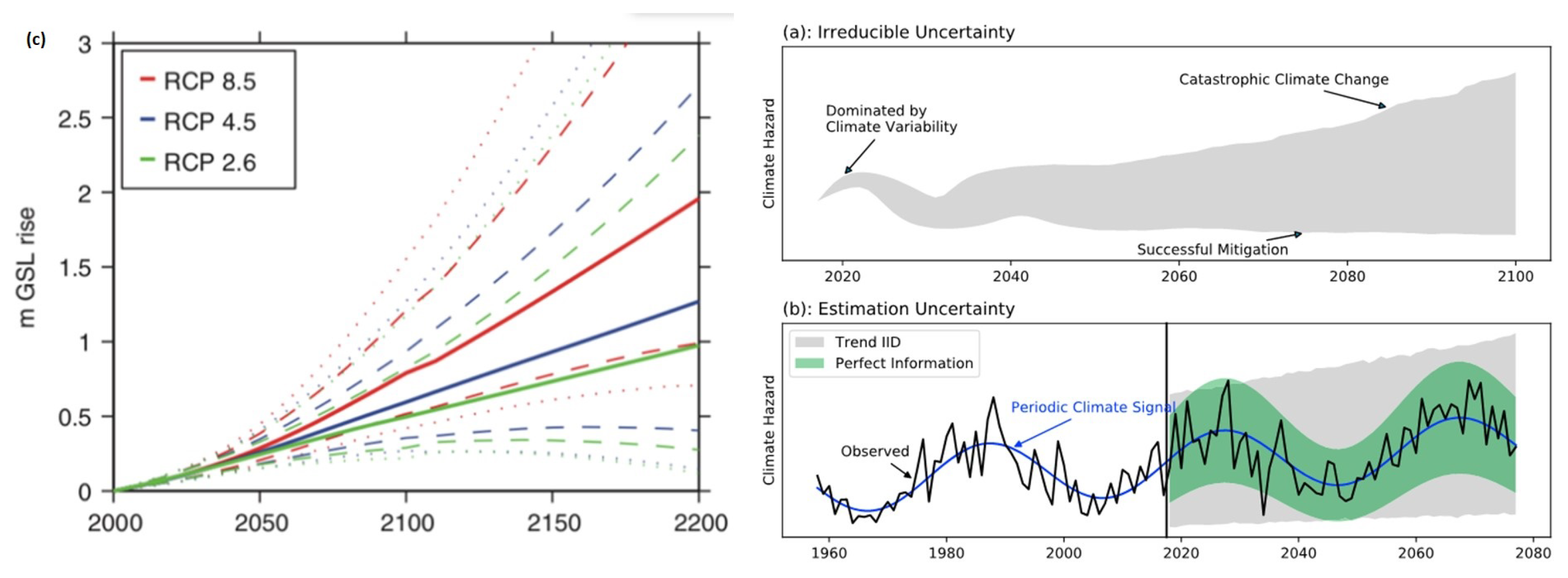
1.1. Source of Uncertainty in Climate Projections

There are different sources of uncertainty in future climate projections. First, although different possible mitigation pathways have been hypothesized as Representative Concentration Pathways (RCP) in CMIP5 or Share Social-economic Pathway (SSP) in CMIP6 [9], there is no assessment of the relative likelihood of these scenarios. This is often considered a deep uncertainty. A second source of uncertainty is due to the different characteristics of Global Climate Models (GCMs). Initial condition, parametric and structural uncertainties affect the GCM simulations which represent climate evolution trajectories that can differ significantly even for the same mitigation scenario [10]. To overcome that problem, an ensemble of models is employed to offer a probabilistic representation of climate projections. Third, in order to explore possible adaptation policies at local or regional scales, the trends of the hydrological variables such as temperature, rainfall or sea level rise need to be projected at a finer spatial resolution than that provided by GCMs. Due to the coarse spatial resolution of GCMs, these hydrological variables are usually biased. For instance, in CMIP5 GCMs, oceanographic processes are simulated with a horizontal resolution coarser than 1 degree of latitude and longitude. This resolution is not sufficient to represent bathymetry variation affecting local processes like coastal currents [11], or small-scale processes like eddies [12]. Furthermore, structural errors in models of the sea level components are probable, as well as, systematic bias caused by missing processes and/or feedback. Ref. [13]. Bias correction methods are also usually adopted to correct daily or monthly rainfall amount projections by GCMs and downscaling methods are used to obtain rainfall projections at finer spatial scale. Both methods add further uncertainties that may be unquantifiable [14,15,16]. Finally, natural variability at decadal or bidecadal scales, could dominate the climate trends and makes the identification of adaptation policies timing very difficult [17]. All these sources of uncertainty are illustrated in Figure 1.

1.2. Metodology Approaches to Adaptation Action Identification

In the literature, a number of methodologies for the identification and the assessment of adaptive actions and works to cope with hydraulic risks in coastal areas under climate change have been proposed in the past [19,20,21]. Among the approaches which explicitly take into account the elements of uncertainty due to climate change are the resilience “bottom-up” approach [22] and the predictive “top-down” approach which is the most used.

Bottom-up approaches do not necessary need climate projections by GCMs. Examples of bottom-up approaches include the policy tipping point [23] and the dynamic adaptive policy pathways [24]. The dynamic adaptive policy pathways method developed by [24] combines some elements of Adaptive Policymaking [25], and Adaptation Pathways [26] methods, like adaptation tipping point, i.e., the point when a particular action is no longer adequate and that triggers a specific condition that requires a new action or plane change. These approaches do not seek to identify the optimal sequence of adaptation actions and their timing.

Top-down methods use climate projections by GCMs as inputs for designing adaptation strategies which might enhance resilience or reduce vulnerability of specific geographic areas to climate change [20,27,28]. Specifically, for coastal areas, [29] developed a top-down type model that integrates multi-objective optimization algorithms and a tree-like decision-making scheme in order to provide the optimal strategy to cope sea level rising. The tree-like scheme coupled with a genetic algorithm evaluates the costs associated with each intervention and the flood risk. The decision tree shows the intervention measures at each planning horizon time step if a threshold value is reached based on the future sea level projections.

The identification of adaptation measure timing provides relevant information which could significantly improve the planning process, and lead to a more efficient use of the economic resource to cope the adverse effects of climate changes. Moreover, approaches should able to schedule the best adaptation actions timing in case of sudden or abrupt climate changes [30].

1.3. The Proposal

In order to address these latter issues, i.e., the need to identify design and timing of defence constructions taking into account the uncertainties in climate projections, including abrupt changes of climate forcing, we propose a multi-objective optimization approach (similar to [29,31]) which integrates hydraulic modelling for simulating flooding and its consequences, in which the timing of the adaptive actions is taken into account among the decision variables of the optimization problem and uncertainties in climate projections are integrated into the definition of objective functions. Multiobjective optimization approach was chosen on the basis of similar considerations as those proposed [29]. Multiobjective optimization methods allows decision makers to choose the preferred solutions among a set (Pareto-optimal set) of trade-off solutions, for example those relative to natural habitat conservation, which can’t be easily expressed in monetary terms [32]. In the present paper, the multi-objective optimization model relies on the definition of two optimality criteria: minimizing the cost of the flood defence infrastructure system and the flooding hydraulic risk for the entire period of climate projections. The formalization of the last optimality criteria, i.e., the hydraulic risk associated to flooding events, relies on the definition of the Expected Annual Damage (EAD) [33]. The EAD accounts for the joint probability density functions of extreme rainfall, storm surge and sea level rise, and the corresponding damages, for a given defence system state identified by the water depth–damage curve related to the land use (CORINE Land Cover) [1]).The uncertainties in future climate projections are treated through time varying probability density functions (Pdf) and are used to compute the EAD. A hydraulic model for the assessment of damage is integrated within the multi-objective optimization algorithm (non-dominated sorting genetic algorithm 2, NSGAII [34]). A case study is presented for the Pontina Plain (Lazio Italy), a coastal region, originally a swamp reclaimed about a hundred years ago, that is rich in urban centers and farms. A set of optimal adaptation policies, belonging to the Pareto curve calculated by the NSGAII, to mitigate the risk of flooding and to aid decision makers are identified for such a case study.

2. Methods

A sketch of the model system is shown in Figure 2. Figure 2 synthetized methodology and related algorithms aimed to identify the size and timing of flood defence constructions to cope with sea level rise, as well as, extreme rainfall regime modification due to climate change. The methodology considers a multi-objective optimization problem, in which both hydraulic risk due flooding and construction costs of flood defence system are minimized for the entire period of climate projections. Hydraulic models are used to calculate the hydraulic variables necessary to the flood damage assessment as a functions of climate forcings and of the state of flood defence systems, taking into account uncertainties in climate projections. Figure 2 also describes decision variables of the multi-objective optimization problem as well as the input ones.

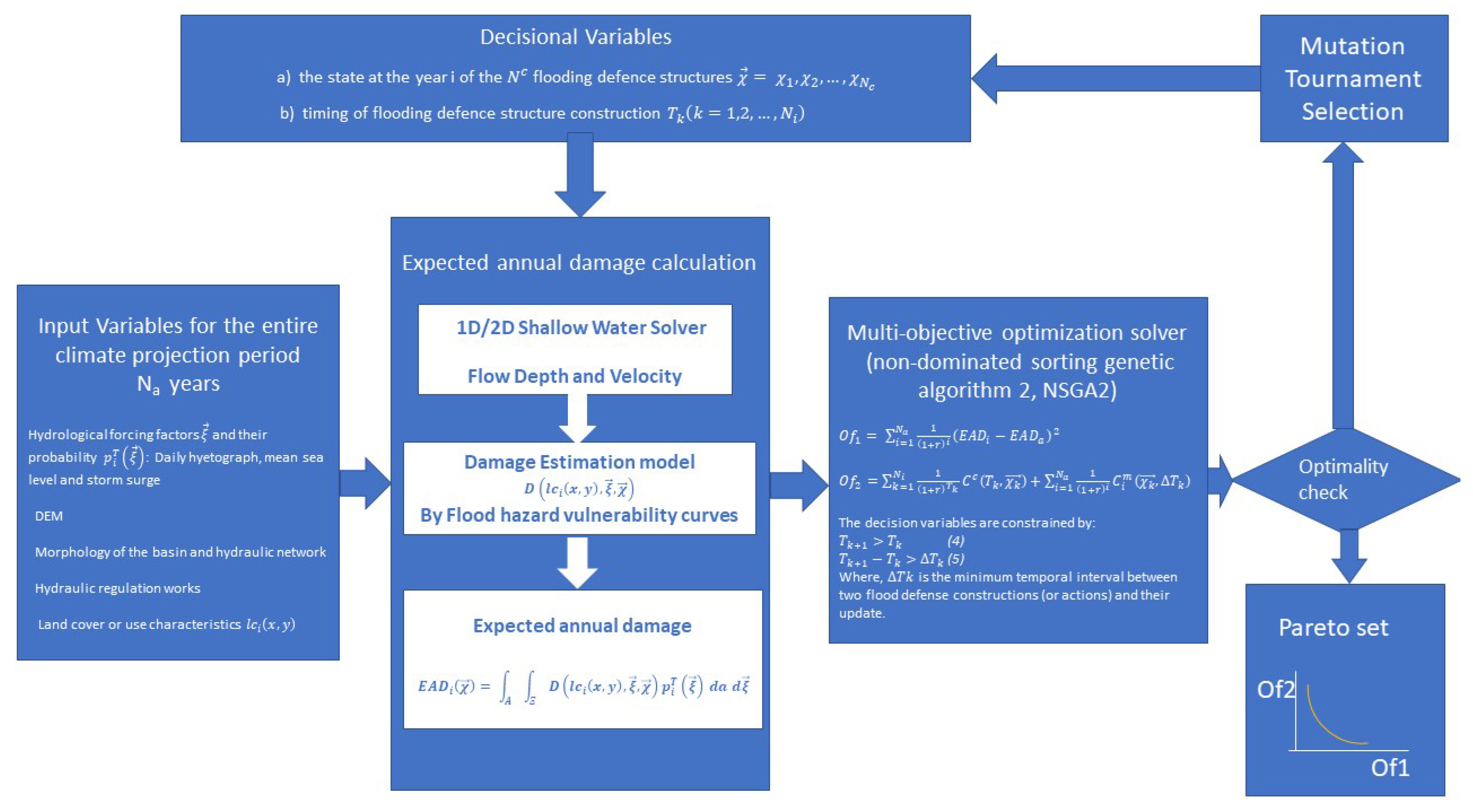
2.1. Multi-Objective Optimization Problem Formalization

Two optimization criteria are defined: (a) minimization of hydraulic risk associated to hydrological extremes for the entire climate projection period; (b) minimization of the cost of the adaptation actions for the same period. Adaptation actions consists of flood defence constructions, as levees, flood retention basins, spillway canals, other actions aimed to reduce exposition to hydraulic risk as for instance retreat strategies [35]. Objective functions for the two optimization criteria are formalized as:

$$O{f}_1=\sum _{i=1}^{N_a}{(\frac{1}{{(1+r_d)}^i}EA{D}_i-EA{D}_a)}^2$$

(1)

$$O{f}_2=\sum _{k=1}^{N_i}\frac{1}{{(1+r_c)}^{T_k}}{C}^c+(T_k+\overrightarrow{{\chi }_k})+\sum _{i=1}^{N_a}\frac{1}{{(1+r_c)}^i}C{}_i^m(\overrightarrow{{\chi }_k}+\Delta T_k)$$

(2)

The flooding hydraulic risk objective function Equation (1) is constructed with reference to the concept of Expected Annual Damage (EAD). The EAD can be expressed as the integral of the probability of not exceeding certain dangerous events, multiplied by the consequences of the event [36]:

$$EA{D}_i\left(\overrightarrow{\chi }\right)={\int }_A^{}{\int }_E^{}D(l_{c_i}(x,y),\overrightarrow{\xi },\overrightarrow{\chi })p_i^T\left(\overrightarrow{\xi }\right)dad\overrightarrow{\xi }$$

(3)

where $D(l_{c_i}(x,y),\overrightarrow{\xi },\overrightarrow{\chi })$ is the damage depending on: (a) land cover or use characteristics $l_{c_i}(x,y)$ being x, y the coordinate of a generic point of the domain representing the region considered; (b) the probability density $p_i^T\left(\overrightarrow{\xi }\right)$ at the i-th year of the $N^c$ hydrological forcing factors $\overrightarrow{\xi }=\overrightarrow{{\xi }_1},\overrightarrow{{\xi }_2},\dots ,\overrightarrow{{\xi }_{N_c}}$, potentially able to cause flooding; (c) the state at the year i of the $N^D$ flooding defence structures $\overrightarrow{\chi }=\overrightarrow{{\chi }_1},\overrightarrow{{\chi }_2},\dots ,\overrightarrow{{\chi }_{N^D}}$. The EAD accounts both the probability density function of the forcing hydrological factors and the damage due to flooding associated with them depending on the intensity of extreme events and of the state of flood defence structures. In Equation (1), $EA{D}_i$ is Expected Annual Damage (i = 1, 2,…, $N_a$), $N_a$ the number of the years of climate projection, $r_d$ and $r_c$ are discount rates related to the first and second objective function respectively, $EA{D}_a$ the Acceptable Expected Annual Damage. We define as acceptable $EA{D}_a$ as the maximum value of EAD that a community can tolerate, in relation to its exposition, vulnerability and hazard. In principle $EA{D}_a$ should be equal to zero, i.e., a community would not want suffer any kind of damage due to flooding. But since zero risk is unrealistic, a community can bear exceptionally flooding producing limited damage to things or building, no casualties and so on. In this sense the acceptable $EA{D}_a$ could be thought as a reference acceptable target for the community, not varying in time. The formalization of the $O{f}_1$ in Equation (1), therefore is a metric representing the distance from such target. The formalization of $O{f}_1$ by Equation (1) is rather general and could also be used for defining other objective functions including those related to assess of intangible damage or related to environmental quality or natural habitat targets which can’t easily expressed in monetary terms [31]. In Equation (2) $C^c$ is the cost of the $N^D$ flood defence constructions and other adaptive actions $\overrightarrow{\chi }=\overrightarrow{{\chi }_1},\overrightarrow{{\chi }_2},\dots \overrightarrow{{\chi }_{N_D}}$, at the time $T_k(k=1,2,\dots ,N_i)$ where $N_i$ number of horizon times in which the climate projection period is divided, $C_m^i$ is the annual maintenance costs of the flood defense constructions depending on the type of flood defence adopted, and the timing between two succeeding constructions. $\Delta T_k=T_k-T_{k-1}$. In the multi-objective problem formalized in Equations (1)–(3), $\overrightarrow{\chi }={\overrightarrow{\chi }}_1,{\overrightarrow{\chi }}_2,\dots \overrightarrow{{\chi }_{N_D}}$ and $T_K(K=1,2,\dots ,N_i)$ are the decision variables, $l_{c_i}(x,y)$ are the state variables,$\overrightarrow{\xi }$ and $p_i^T\left(\overrightarrow{\xi }\right)$ are the input variables. The decision variables are constrained by:

$$T_{k+1}>T_k$$

(4)

$$T_{k+1}-T_k>\Delta T_{min}$$

(5)

where, $\Delta T_{min}$ is the minimum temporal interval between two flood defence constructions (or actions) and their update. We also impose that once a construction is realized at the time $T_k$ it can’t remove at the time $T_{k+1}$ but only update if necessary, except for the case in which flood defences can be destroyed by the occurrence of a large event as, for instance, that able to produce an overflow of levees. In the latter case the cost the entire reconstruction of flood defence is taken into account. The other decision variables are also included within an interval of reasonableness, for instance the increase of the embankments will be selected within an predefined range from 0 to a maximum levee crest height.

The probability $p_i^T\left(\overrightarrow{\xi }\right)$ in Equation (3) is a resulting probability density function that accounts for the probability density of each forcing factor ${\xi }_j(j=1,2,\dots N_c)$ as well as the changes in probability functions of the forcing factors associated to the ensemble of GCMs simulations within a for each future climate scenarios. If the forcing factors are mutually independent, for a single climate scenario, the probability density function is given by the product of probability of every single event. If the forcing factors are not independent, a different methodology could be used to account for the dependence among the different forcing factors, e.g., bivariate point process method [37]. Furthermore, the probability density function for an ensemble of GCM simulations, as well as the likelihood of different RCP or SSP climatic scenarios have to be taken into account in the definition of $p_i^T\left(\overrightarrow{\xi }\right)$. This allows one to include the uncertainties of future emission scenarios, as well as those in climate modeling.

2.1.1. Discount Rates

In Equations (1) and (2) two different discount rates $r_d$ and $r_c$ are considered. In the context of climate change policy making, they are very important in understanding how much society today should invest in trying to protect vulnerable areas, limiting the impacts of climate change later in the future [38]. Depending on the context, discount rates can assume different meanings [39]. In the specific case proposed in the present study, $r_d$ in Equation (1) is as a measure of the relative importance of negative consequences produced by flood events in term of hydraulic risk occurring at different points in time. It therefore can be thought as how we weight risks due to future events within an intergenerational pact. Higher is $r_d$, lower is our hydraulic risk assessment at future times for the same hydrological event; $r_d$ equal zero is equivalent to assume a temporal independence of hydraulic risk assessment.

The discount rate $r_c$ in Equation (2), that is related to the flood defence construction costs, depends on general condition of economy in a more close relation with the market dynamics. Since our formulation of the multi-objective problem allows to formalize the objective functions in different measurement units, eventually incommensurable, the distinction between the two discount rates appears to be appropriate. Furthermore it allows a more flexible approach to the problem.

2.1.2. Damage Assesment

The term $D(l_{c_i}(x,y),\overrightarrow{\xi },\overrightarrow{\chi })$ in Equation (3) accounts for the damage due to inundation depending on the state of land cover and the defence constructions, and on the entity of forcing factors. The damage $D(l_{c_i}(x,y),\overrightarrow{\xi },\overrightarrow{\chi })$ is estimated as follows. The direct damage associated with the physical impacts of a hazard is estimated by unit damage functions or Stage-Damage functions, which are conceptually similar to the fragility curves used in other disciplines. In the event of flooding, the damage functions are determined by the use of a specific relationship between the characteristics of flood and the extent of the economic damage referred to a specific type of asset exposed [40]. The procedure for estimating direct damage has 3 components: (1) The characteristics of the assets exposed through the analysis of the information on land use by satellite data [41]; (2) the characteristics of the flood represented by depth and extension of the flooding: (3) the combination of the (1) and (2) with the depth curve-damage in order to stimulate the extent of the damage with respect to the value of the exposed asset. Vulnerability and exposure of each point of the considered region is featured by the term $l_{c_i}(x,y)$ which is assumed to change from year to year as a consequence of modification of land use or increase/decrease of urbanization or population. The physical characteristics of the territory and the value of vulnerable assets (1) are represented by the digital terrain model (DTM) and by the satellite land use data (CORINE Land Cover), respectively. The extent and depth of the flooding were obtained by numerical hydraulic simulations, for given rainfall intensities and sea levels. The data thus obtained are translated into a damage index or the percentage of the value of the asset that is lost, through the depth-damage curves [42]. Several countries have developed standardized methods for estimating flood damage. An example is the HAZUS methodology developed in the USA [43], the guidelines for cost-benefit analysis (CBA) developed in the UK [44], and Australia (Bureau of Transport Economics, 2001). The model we chose was HAZUS as it provides an estimate of a large variety of damages, direct and indirect. For each calculation cell of 100 ${\mathrm{m}}^2$, the damage constitutes in the value in Euro of the damage caused by type of asset according to the depth of the flooding.

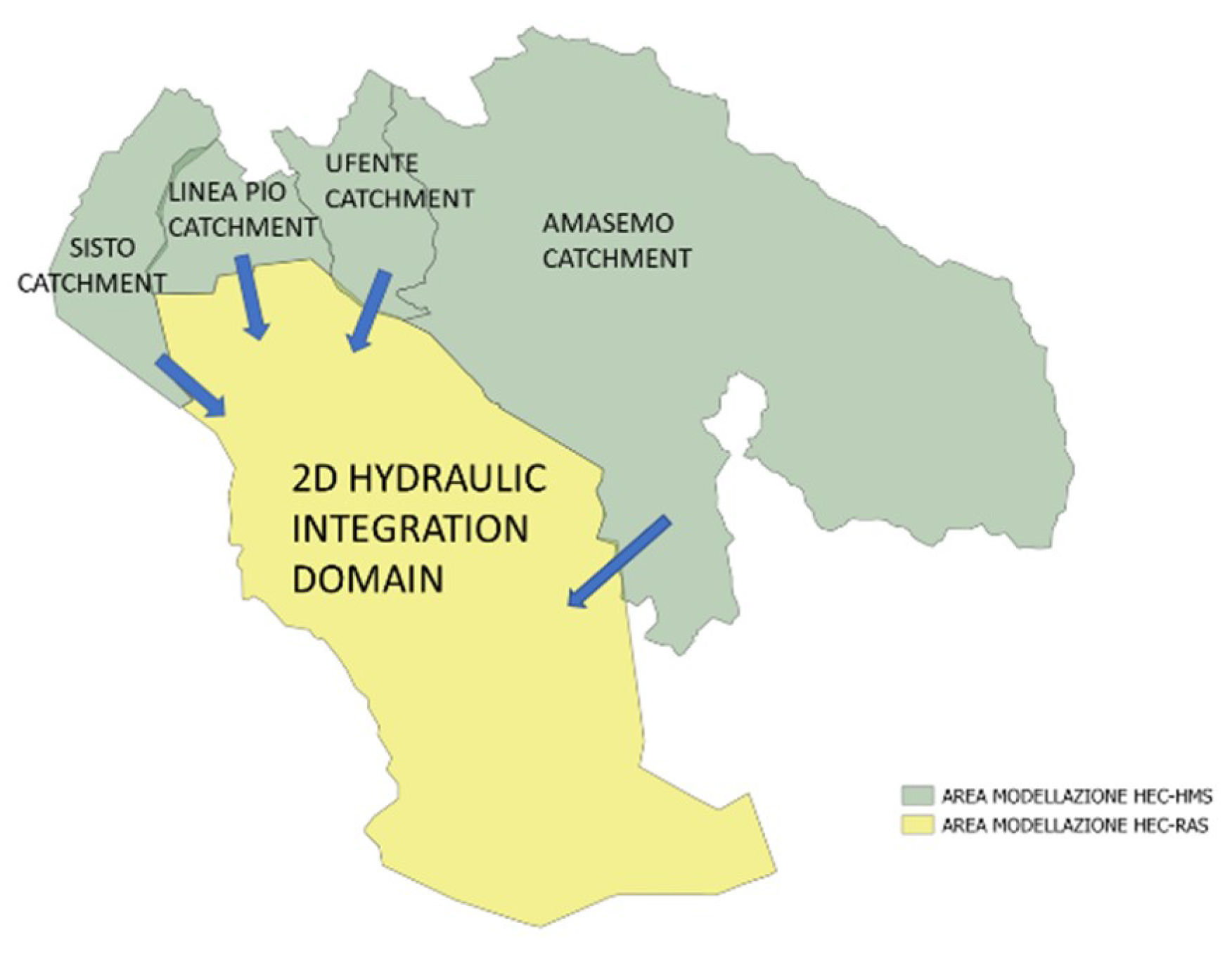
2.1.3. Hydraulic Models

Flood damage assessment requires knowledge of the hydraulic characteristics of the flooding—water depth, flow velocity, flooding persistence. These are obtained by hydraulic simulations forced by direct application of rainfall, as well as, boundary conditions due to storm surge and sea level rise. In this paper, for the study case, two different hydraulic models are used: (a) a 2D hydraulic model, the USACE Hydrologic Engineering Center’s River Analysis System (HEC-RAS 5.0.7); (b) a fast simplified hydraulic model. The first model is a public domain software that meets the minimum requirements of National Flood Insurance Program as required by FEMA (https://www.fema.gov/hydraulic-numerical-models-meeting-minimum-requirement-national-flood-insurance-program). A recent FEMA report (https://www.fema.gov/media-library-data/1561469561757-6fed6a4fd077673f684920b9ad5a0e53/RapidResponseFloodModelingFinalReport.pdf) shows that the model produces results with higher precision (standard deviation) and predictive value (correlation) than other models.

The equations in HEC-RAS are solved using an implicit Finite Volume algorithm. This algorithm allows the use of a structured or unstructured computational mesh. Local thickening of computational mesh can be applied by breaklines, added along levees, buildings, roads, and in abrupt slope change. One of the advantages of using HEC-RAS is the possibility to simulate the presence of gates, pumping stations, and other hydraulic devices for flow maneuver. For very large domains, the 2D HEC-RAS code can be coupled with HEC-HMS which is a physically based and conceptually semi-distributed model designed to simulate rainfall-runoff processes to provide flood hydrographs generated externally from the 2D integration domain.The fast simplified hydraulic model [45] models the hydraulic network and the flooplain using three elements: the main river hydraulic networks, the storage areas representing the basins, and the ideal channels connecting the storage areas to points of the rivers belonging to the hydraulic network. The 1D Saint-Venant equations are used to simulate the flow along the rivers which belong to the hydraulic networks. The temporal trend of water level over the storage areas is calculated by the continuity equation, which is a function of the flows entering or going out from the ideal channels and of the rainfall amount directly falling over the area.

2.1.4. Flood Defence Construction and Maintenance Costs

To evaluate the objective function expressed by Equation (2) construction and maintenance costs of flood protection structures have to be evaluated. Such costs include the construction of fill, columns, flood walls, levees, and flood shields or closures, as well as, that of auxiliary materials and activities that are required to assure that the primary flood proofing elements function properly. Examples are the cost for providing access to buildings on fill, or interior drainage for areas enclosed by levees or floodwalls. We considered two kind of works: levees in the most critical zones of the hydraulic network, and the creation of flood expansion areas ruled by weirs. In order to estimate the costs of raising the banks, reference is made to the study conducted by [46], which estimate between 4.5–12.4 million Euros per km of length and per meter of raising the embankment in rural areas. In the present study a unit cost of C = 4.5 million Euros/km per meter of embankment elevation will be considered.

For every planning horizon the total cost of the riverbanks rise is calculated using the following equation:

$$C_{arg}(t,l_2)={\delta }^t(l_2\left(t\right)\ast C\ast L)$$

(6)

where L is the length of the entire network of embankments, around 35 km. Maintenance costs, €100,000 per kilometer to be spent every 10 years, were provided by the Reclamation Consortium Office. The cost of expansion areas was evaluated as lost space to most productive uses, the amount is €5000 per hectare for each year in which the expansion area is flooded.

2.1.5. NSGAII Genetic Algorithm

The multi-objective optimization problem of Equations (1)–(5) is solved by the NSGA II genetic algorithm. Genetic algorithms mimic the Darwin’s theory of natural selection: a population represents a group of solution points. A generation represents algorithm iteration. A chromosome is equivalent to a component of the design vector. In accordance to these definitions genetic algorithm deals with a population of points, and hence multiple Pareto optimal solutions can be obtained from a population in a single run. Random number and information from previous iterations are combined to evaluate and improve a population of points, and then to select non-dominant solutions. In this paper the non-dominant-sorting genetic algorithm II [47], NSGA II, is used, which has been applied successfully to many optimization problems. This algorithm uses tournament Goldberg and Deb [48], simulated binary crossover (SBX) [49], mutation operator and crowding distance for diversity preservation. The original NSGA II Matlab code has been adapted to the specific multi-objective optimization problem above described.

2.2. Probability Density of Hydrological Forcing Factors

In order to calculate the EAD of Equation (3) it is necessary to estimate the probability density function $p_i^T\left(\overrightarrow{\xi }\right)$ taking into account the statistical independence or the possible statistical dependence among the different hydrological forcing factors. Generally, heavy daily rainfall amount and storm surge due to wind set-up and low atmospheric pressure are statistically dependent, while the average sea level rise, as a consequence of climate change, can be assumed statistically independent from the above cited forcing factors [50,51]. Therefore, in Equation (3) we express the probability density function as:

$$p_i^T\overrightarrow{\xi }=p_i^T({\xi }_1,{\xi }_2)p_i^T\left({\xi }_3\right)$$

(7)

where $p_i^T({\xi }_1,{\xi }_2)$ and $p_i^T\left({\xi }_3\right)$ are the probability density functions of the statistical jointly variables heavy rainfall amount ${\xi }_1$ and storm surge ${\xi }_2$ and of the statistical independent variable sea level rise ${\xi }_3$.

2.2.1. Heavy Rain and Storm Surge Joint Probability

The estimation of the joint probability of the occurrence of intense rain and storm surges is extremely important [37] because even a weak dependence can have significant implications in the estimation of the hydraulic risk [52]). Indeed, heavy rainfall and storm surge are often caused by similar atmospheric conditions such as, low atmospheric pressure and strong winds that cause storm surge. Several methods of multivariate statistical analysis exist to estimate the dependence of such events, including the Point Process Method [53,54]. For the estimation of the probability distribution $p({\xi }_1,{\xi }_2)$ the “logistic model” can be applied [37]:

$$p({\xi }_1,{\xi }_2)=exp-{({\xi }_1^{-1/\alpha }+{\xi }_2^{-1/\alpha })}^{1/\alpha }0<\alpha <1,{\xi }_1>0,{\xi }_2>0$$

(8)

where ${\xi }_1$ and ${\xi }_2$ represent the extremes of the bivariate vector consisting respectively of daily rainfall amount and daily storm surge levels, which is assumed to follow the standard Frechet distribution. The parameter $\alpha$ indicates the dependence between the two extremes with $\alpha \to 0$ complete dependence and $\alpha \to 1$ independence. The method used involves identifying the rainfall and storm surge intensity thresholds and estimating the Generalized Pareto Distribution (GPD) of the margins. Then using GPD parameters, the entire dataset is transformed to have the standard Fréchet margins [55]. After the transformation of the Fréchet margins into radial and angular components (r, w), the joint threshold $r0$ is selected. The $\alpha$ parameter is estimated through a likelihood function constructed from the spectral density $h\left(w\right)$.

$$h\left(w\right)=\frac{1}{2}({\alpha }^{-1}-1){\left[w(1-w)\right]}^{-1-1/\alpha }{[w^{-1/\alpha }+{(1-w)}^{-1/\alpha }]}^{\alpha -2}$$

(9)

The inference for the Point Process Method is based on a likelihood function constructed from the spectral density $h\left(w\right)$:

$$L(\alpha ;({\xi }_1,{\xi }_2)\dots ({\xi }_n,{\xi }_n))=\prod _{j|r_j>r_0}h\left(w_j\right)$$

(10)

The joint probability of the events will be considered for each year of the time horizon considered. The model is calibrated using the data relating to the accumulated daily rainfall for 20 years of records of rainfall stations present in the study area.

2.2.2. Mean Sea Level Rise Projections

The future mean sea level until 2200 can be derived from [18,56,57]. Using a model ensemble, ref. [18] provide a method for obtaining probabilistic projections of sea level rise both on the global scale and on the local scale considering the individual contributions due to the melting of both the polar ice caps and glaciers. The projections use 3 RCP scenarios, 8.5, 4.5 and 2.6. In order to obtain local sea level rise projections, the model requires the aggregation of the individual components that influence the sea level change in every site of interest [58]. Those components are respectively the three ice sheet components (Greenland, West Antartic and East Antartic): (a) the global mean thermal expansion and the ocean dynamic effects based upon the CMIP5 [59] and GCM models; (b) the land water storage evaluated following the approach of [60]; (c) the glacier and ice cap surface mass balance and tectonics. The non-climatic effects can be approximated as linear trends over past century and assumed unchanged, using spatiotemporal Gaussian process model [61]. We use the DP16 projections because they included previously omitted processes such as the hydrofracturing of the ice shelf and structural collapse of high ice cliffs ending at sea, which have the potential to drive a higher sea level rise. Projections of ice sheets for the 21st century are generated from IPCC AR5 projections (IPCC, 2014), used to characterize median and likely ranges of sea-level change, while study carried out by [62] is used to calibrate the shape of the tails. For each RCP, the model employ a multivariate t-distribution of ice mass change with a mean and covariance estimated from the model results of [63]. To calculate global and local sea level projections the model uses 10,000 Latin hyper–cube samples from time dependent probability distributions of cumulative contributions of each individual component [18]. To calculate the probability of increasing of the average local sea level at site of interest (${\xi }_3$), taking into account the different RCP scenarios, we estimated the probability linked to each level of increase for each year by calculating the probability distribution function relative to a sample of 30,000 projections, 10,000 for each RCP scenario considered. Each RCP scenario is assumed as independent from others with a different temporal varying density probability function.

3. Case Study

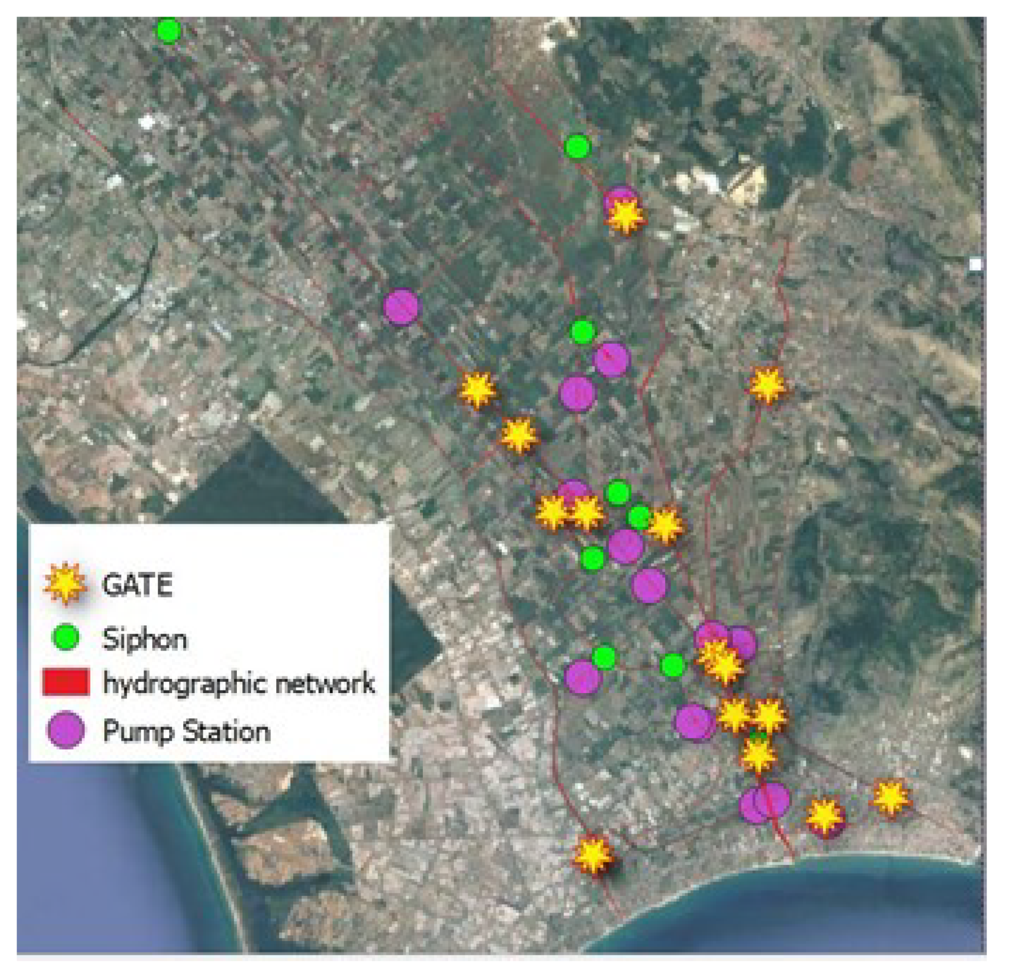
3.1. Site Description

The model developed was tested on the southern area of the Pontine Plain, a recovery area with a surface of 395 ${\mathrm{km}}^2$, originally a swamp, reclaimed in 1920s and located in the south of Lazio region (Italy). The area is densely populated, with a significant presence of agriculture and industrial activities. A natural park, Circeo National Park, aimed to conserve the biotypes and biodiversity typical of wetland environments covers the areas closer to the coast, with the presence of a long coastal dune and a number of coastal lagoons [64]. These social, economic, naturalistic and ecological characteristics, together with the morphological ones, determine a particular vulnerability and exposition of the zone to extreme hydrological events and sea level rise. In fact, vast areas are below the sea level, furrowed by a dense network of canals that are mostly artificial and subject to periodic flooding phenomena due to the concomitance of meteorological phenomena such as heavy rains and local sea level rises due to storm surge. As shown in Figure 3, the area is kept dry by pumping water that accumulates in the most depressed areas by conveying it into a higher altitude network of canals and then discharged into the sea. In addition, maneuvers are carried out by the network operators, such as opening and closing mechanical sluice gates, to prevent excessive water from accumulating inside the channels during emergency periods.

The most important is the Mazzocchio pumping station, which has a maximum capacity of about 30 m${}^3$/s and is used to drain the water that accumulates in the most depressed area of the Pontine plain, with a minimum altitude of up to −3 m above sea level. The area upstream the Mazzocchio pumping station has an extension of about 102 ${\mathrm{km}}^2$ and due to the lower altitude in respect to surrounding basins it results hydraulically connected with downstream hydraulic network only by the pumping. Therefore changes in flow rates and flow depths in the rivers downstream from the pumping don’t affect the flow characteristics of the areas upstream from the pumping station. On contrary the flow rates lifted by Mazzocchio pumping station affects the flow characteristics of the downstream area. A previous study by [45] showed, that during heavy precipitation events, higher pumping flow rates reduce the extension of flooding areas upstream from Mazzocchio pumping station, but it worsens the flooding of those downstream. In the current study case, we explore how to increase the resilience to sea level rise of the drainage network downstream from Mazzoccio pumping station, through both the raising of the embankment elevation along the most vulnerable part of the drainage network and the construction of flood expansion areas ruled by weirs along the channels. In this context an analysis has been conducted with the aim to verify how an increasing of the pumping power of Mazzocchio station could reduce the extension of the flooding in the areas upstream from the station and how such increase could affect the flooding in the downstream zones. Therefore simulation were carried out for two different global pumping power for Mazzocchio station: the current ones with 6 pumps having a 6 m${}^3$/s flowrate and an hypothetical configuration with the same number of pumps but able to lift up to 9 m${}^3$/s.

3.2. Data

The data used in the present study are the amounts of daily rainfall in the study area, the sea level, the ground level, the land use and the channel network morphological characteristics.Above mentioned data can be downloaded at github.com/project.

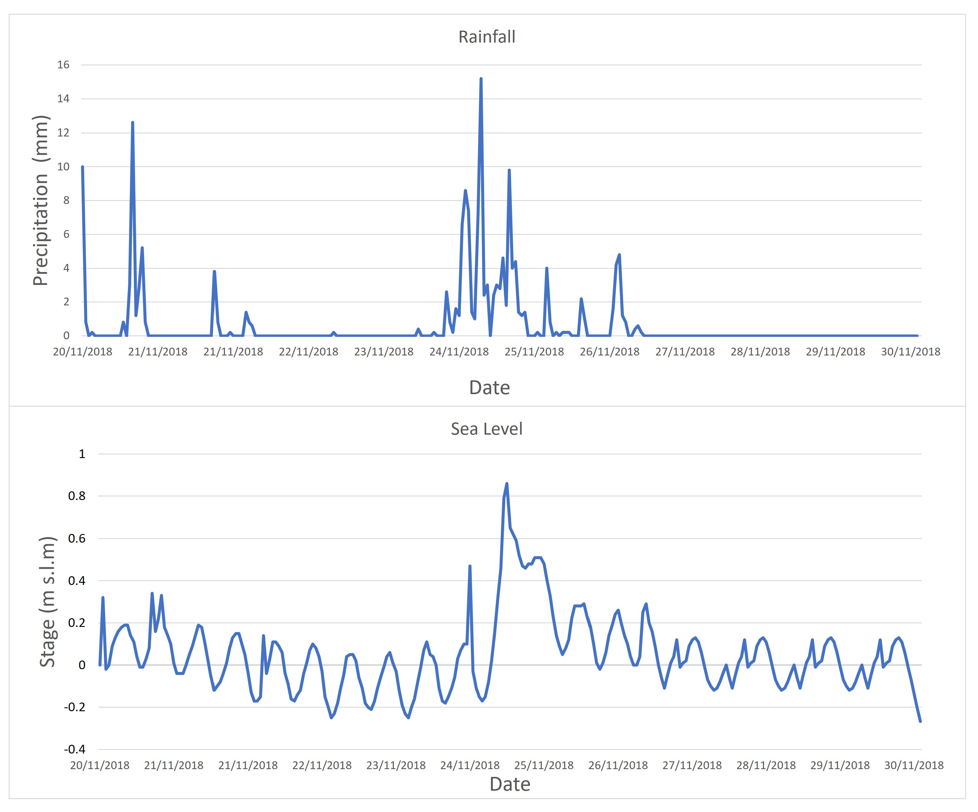
3.2.1. Rainfall Data

Rainfall data recorded from five rainfall stations present in the study area were used. Four rain gages, whose coordinates are shown in

Table 1. Coordinates Rain Stations.

Rain Gauge	Lon	Lat
Latina	12.8313442	414623368
Lenola	13.4401114	41.4051557
Ponte Ferraioli	13.0958461	41.4643082
Terracina	131255395	41.2848763
Mazzocchio (Pontinia)	13.136856	41.397645

, provided daily precipitation amount from 1 January 1980 to 31 Decmber 2000. The first station, located in the municipality of Latina (12${}^{\circ }$58${}^{\prime }$12${}^{″}$ 41${}^{\circ }$25${}^{\prime }$12${}^{″}$) provided hourly rainfall amount time series for a shorter period (since 2009). Using the 10 years long hourly rainfall time series, and applying the method developed by [65], synthetic hyetographs were generated which distribute the total rainfall amount in 24 h according to a statistical distribution obtained from the hourly rainfall data. In fact, a previous study [45] has shown that 24-h-long heavy rainfall (with a daily rainfall amount greater than 100 mm) has, in the past, induced serious flooding in the examined site. Ref. [45] is reported a detailed description of the methodology used to construct the hyetographs for the study case. The daily rainfall amount time series were used to obtain the joint probability between extreme rainfall and storm surge in according to the method described Section 2.2.1.

3.2.2. Storm Surge Data

Since direct measurements of storm surge along the coast were not available for the site, we reconstructed the sea level time series from 1 January 1980 to 31 Decmber 2000. using the time series of the wind speed and direction and sea level pressure for the area of interest (Lat 39.75–42, Lon 12–14.25). Sea level is a combination of the component due to the action of the wind (wind set-up), of the astronomical tides (Boon, 2020) and of the atmospheric pressure acting on the sea free surface. Storm surge levels are calculated starting from the pressure data on the mean sea level and zonal and southern wind intensity obtained from the ERA-Interim model [66]. In order to derive the wind set-up, we applied the relationship and coefficient obtained by [67]:

$$S=\frac{K_p{L}_p{U}^2}{g(D-h-S)}ln\frac{D}{h+S}$$

(11)

where:

• U = wind speed (m/s) at 10 m. over the sea surface;
• D = limit depth of the continental shelf (~200 m);
• $L_p$ = continental shelf extension (m);
• h = depth where storm-surge is calculated (m);
• g = gravity acceleration (9.81 m/s²);
• $k_p$ = coefficient equal to $3\times {10}^{-6}$.

For the specific coastal zone eastern-southerly winds produce higher storm surges which increase due to the contribution of sea level pressure and astronomic tide. Usually, extreme meteorological events in the considered zones last from one to three days, thus also the maximum tidal amplitude has to be taken into account as a further component to the storm surge. To calculate the height of the sea due to astronomical tides the model developed by [68]. The measurements from which we obtained the trend of the astronomical tides refer to the recordings made by the Gaeta tide gauge (LAT 41${}^{\circ }$12${}^{\prime }$35.97${}^{″}$, LON 13${}^{\circ }$35${}^{\prime }$23.05${}^{″}$). The range of tidal amplitude in that coastal area result equal to ±200 mm.

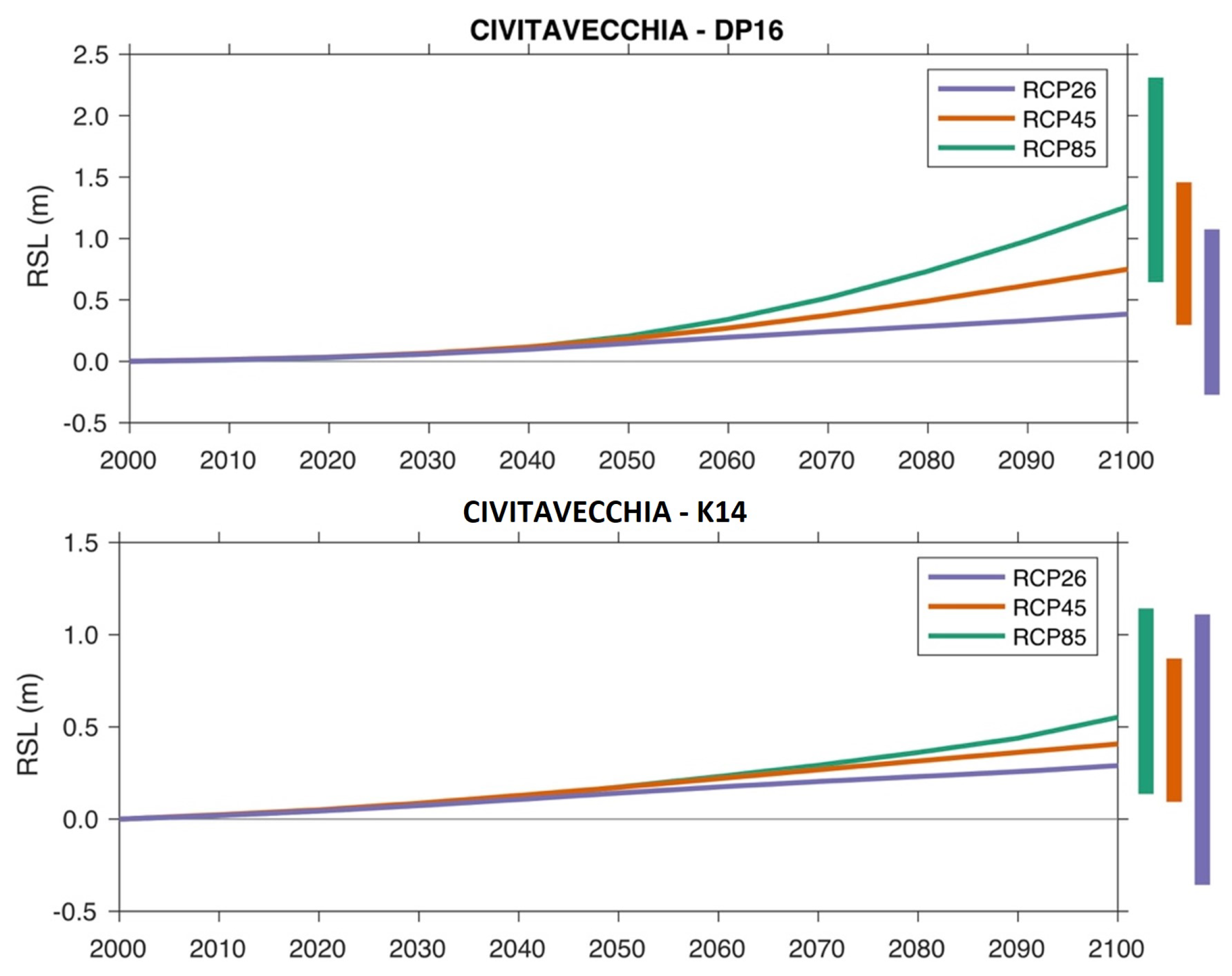
3.3. Sea Level Rise Projections

To obtain the projections for raising the local average sea level, we used the data recorded in Civitavecchia tide gauge which is located in a zone close to that of the study case and having very similar morphological characteristics. Two different projections of mean sea levels were calculated referred to [57] (DP16) and [18] (K14). As shown in Figure 4, the two projections show a substantial variation of the median sea level rise, with regard to the worst-case scenario (RCP 8.5), of more than 1 m in 2100. The two scenarios considered differ mainly in the contribution of the hydro-fracturing of the Arctic ice sheets introduced by [57] in the model developed by [18].

4. Results

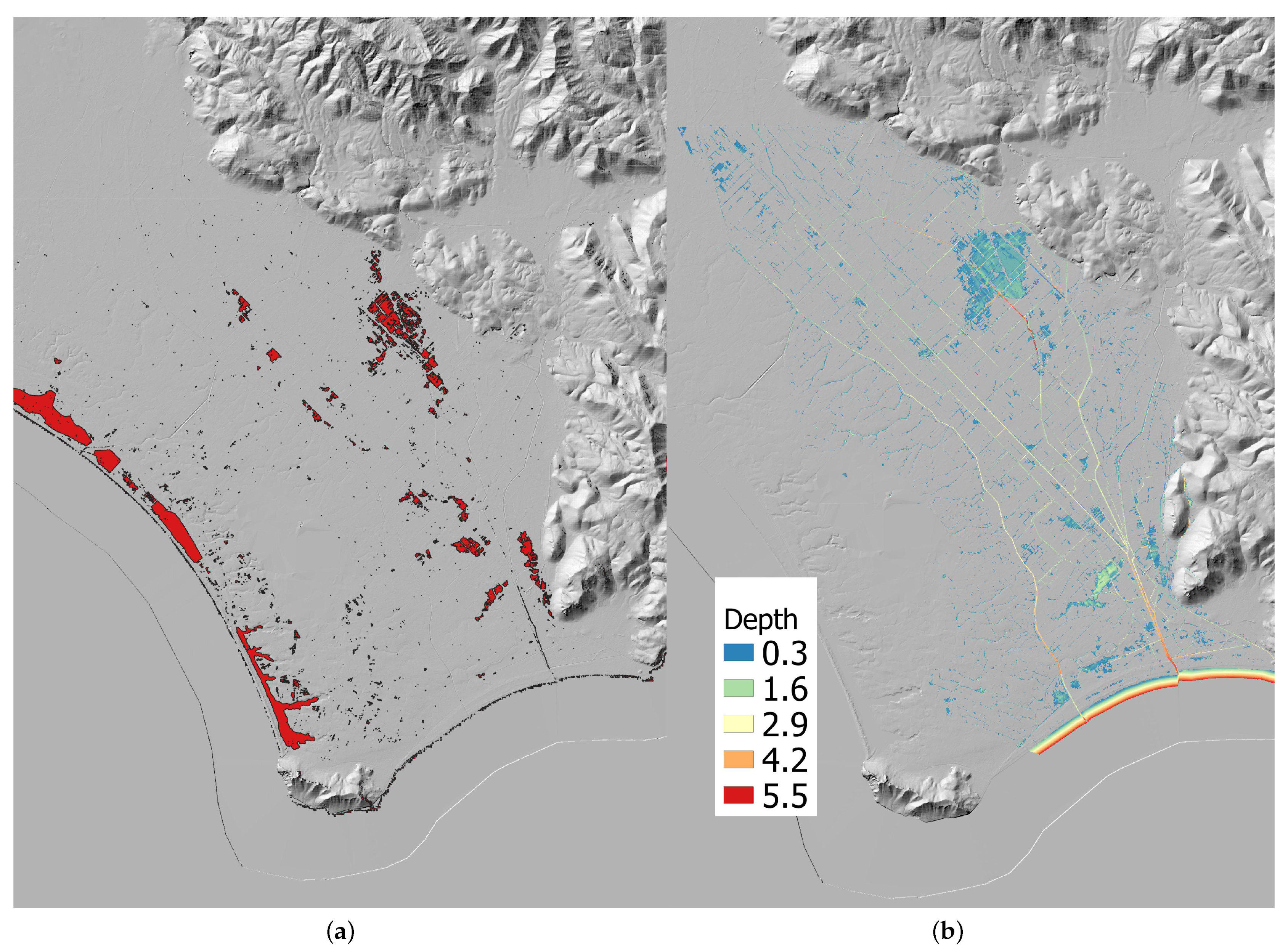
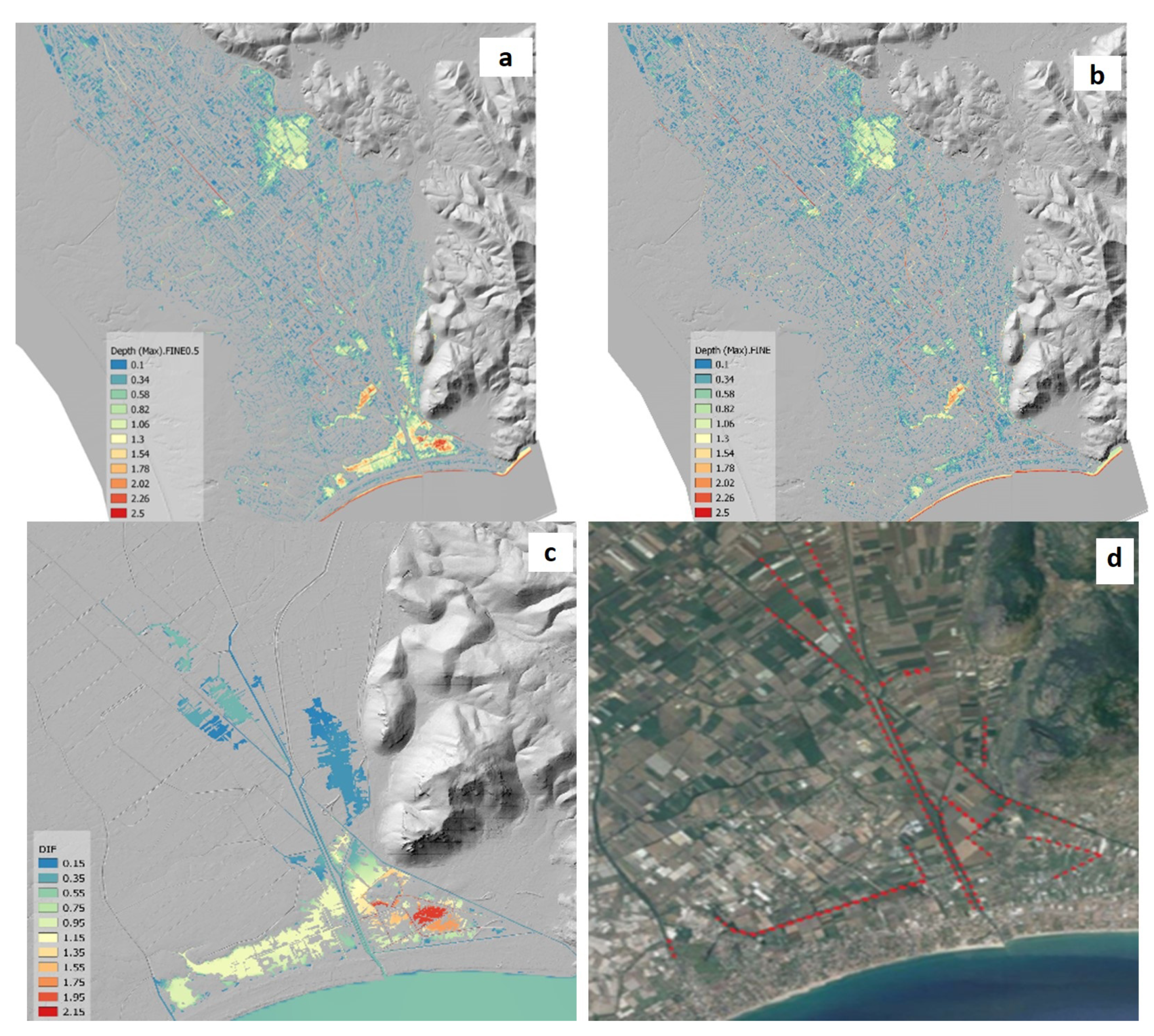
4.1. Hydraulic Simulations

In order to analyze the hydraulic response of the hydraulic network and of the surrounding floodplains of the area and to identify the critical zones to flooding 2D hydraulic simulations were carried out. Due to the large dimensions of the catchments feeding the hydraulic network the integration domain was divided as shown in Figure 5.

Hydrographs at the closing sections of the upstream basins were obtained applying rainfall runoff models. These hydrographs were applied as inputs to the 2D hydraulic model. The rainfall-runoff models as well as the 2D hydraulic model were calibrated using data from the hydrometric and meteorological monitoring system, and Sentinel I satellite image of flooding, recorded during the event of 25 November 2018. The monitoring system consists of eleven hydrometric stations and two meteorological stations, which collect the data and return the hourly averages relating to the water tie, to rainfall, to the wind intensity and direction, atmospheric pressure, etc.

Figure 6a,b show the hyetograph and the sea level trend recorded during the event of 25 November 2018 respectively, and applied as boundary conditions to the rainfall-runoff model as well as to 2D shallow water hydraulic model. Rainfall-runoff models for each of the basins sketched in Figure 5, were calibrated by varying the saturation factor k as defined by Şen (2008)

$$\frac{dR}{dP}=(1-e^{-kP})$$

(12)

where $\frac{dR}{dP}$ is the runoff rate, being R the runoff and P the precipitation amount. Typically, the value of k ranges between 2.54 to 12.7 (mm${}^{-1}$) depending on the land cover and of hydrologic soil group. In the present study case uniform values of k were assumed for the entire integration domain. Figure 7 shows such comparation.

To calibrate k in the part of the basin simulated by 2D hydraulic model, the fit between the flooding areas detected by satellite images $A_{obs}$ and those obtained by simulations $A_{sim}$ was evaluated by the following index:

$$I\left(k\right)=\frac{A_{obs}\cap A_{sim}\left(k\right)}{A_{obs}\cup A_{sim}\left(k\right)}$$

(13)

The best value of the saturation factor k was identified as the one that yields the maximum value of $I\left(k\right)$. In Equation (2) refers only to the flooding areas which are detected by satellite. Therefore coastal lakes and other water bodies, as well as, vegetate and dense urbanized areas were removed ([69,70,71]). After model calibration, a number of simulations were carried out, forced by the same rainfall of the event 25 November 2018, with different values of the pumping rates in Mazzocchio station and of the sea level rise, with the goal to identify the most vulnerable areas to flooding and the type and location of the flood defence constructions, as levees, dikes or flood expansion areas. In order to calculate the damage function $D(l_{c_i}(x,y),\overrightarrow{\xi },\overrightarrow{\chi })$ of Equation (3), related to flooding in the study area, simulations were carried out using the fast simplified model, which takes into account the entire domain shown in Figure 5, and whose parameters were calibrated with reference to same above mentioned heavy rainfall event used in 2D simulations. Hydraulic simulations were carried out considering rainfall events lasting 24 h. Then, 24 h rainfall amounts were distributed hourly according to the synthetic hytographs. Hydraulic simulations were carried out offline to reduce the computation time. Different hydraulic construction states were considered, raising embarkment level in the range of 0 and 4 m, with longitudinal weir level ruling flood expansion areas varying between 2 and 6 m above mean sea level. The scenarios considered consist of five rainfall intensities, five storm surge levels and five average sea level rise scenarios combined to form 625 different simulations with each combination of boundary conditions. For the simulations, extreme rains of intensity from 30 mm per day to 150 mm per day, storm surge levels from 20 cm per day to 100 cm per day and increases in the average marine level from 20 cm to 200 cm were considered. The most depressed areas of the domain are kept dry by groups of pumping stations whose flow rates were related to the water level in the upstream storage tank.

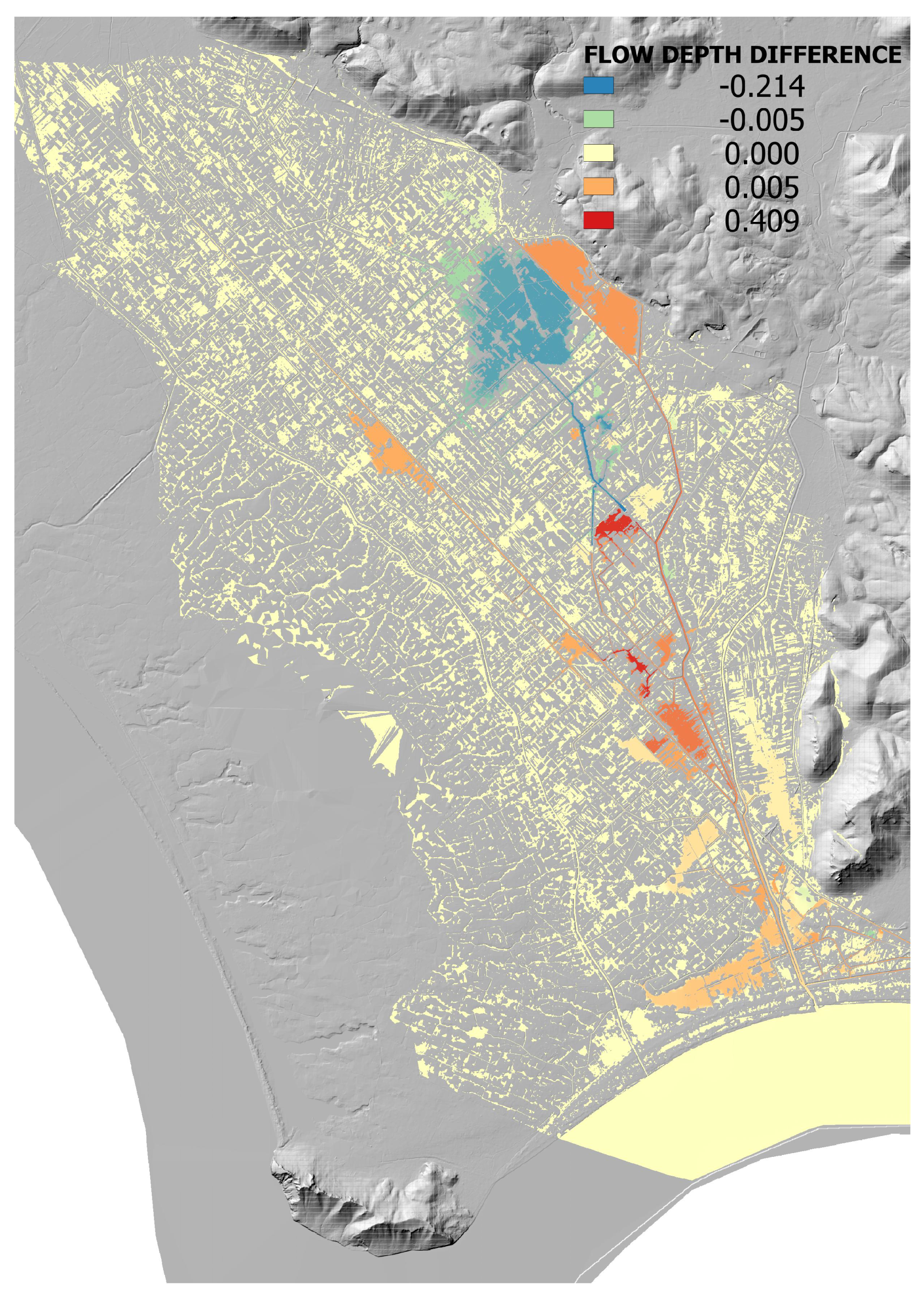
4.2. Effect of the Increase of Pumping Power at Mazzocchio Station and Identification of Flood Defence Constructions by 2D Hydraulic Model Simulations

For the event of 25 November 2018, Figure 8 shows the maximum flow depth difference between the simulated configuration with 9 m${}^3$/s pumping flow rate for each pump of the Mazzocchio Station and with 6 m${}^3$/s ones. In simulations the switch-on and switch off of different group of pumps were considered as a function of different free surface levels in the tank upstream of the Mazzocchio pumping station. The increase of pumping reduces the maximum flow depth of about 0.20 m. in the zones upstream from Mazzocchio Station but increases it in the downstream area up to 0.4 m. in the most depressed zones.

With the aim to identify the areas most prone to flooding, and to define the type and locations of flood defence constructions, a number of hydraulic simulations for different average sea level rise were carried out, applying the same hyetograph of the event of 25 November 2018, as well as the same storm surge trend. Figure 9a–d shows the comparison between the water depth field at the instant of maximum flooding for the current average sea level and that assuming an average sea level rise equal to m. 0.5. As shown in Figure 9c there is a notable worsening of flooding conditions, especially in the urbanized region closer to the coastal line and where there is the convergence of the main watercourses.

To defend such a region different kinds of flood disaster risk reduction measures could be adopted [72]. Here, as shown in Figure 9d, we consider raising the embankment elevation along the drainage network crossing the most vulnerable areas and the construction of flood expansion areas, upstream from such areas, ruled by the level of weir along the channels.

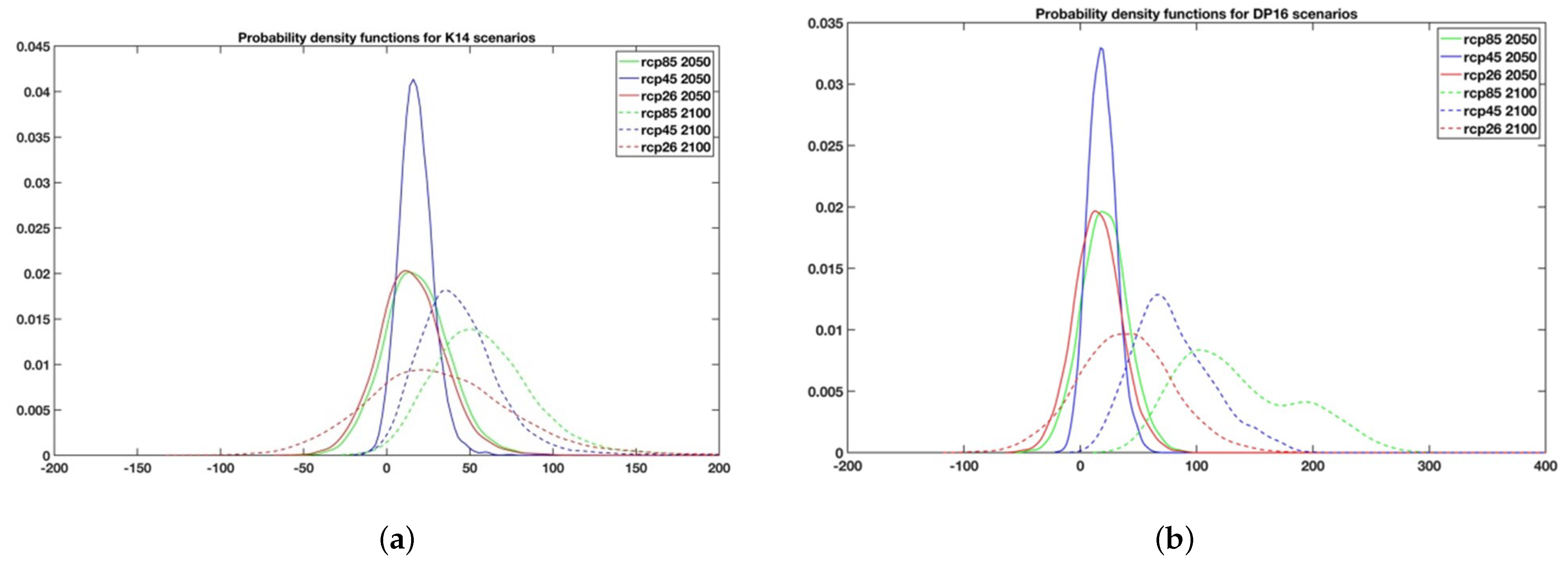
4.3. Probability Density Function for Sea Level Rise Scenarios

To calculate the probability of raising the local sea level, 10,000 simulations were carried out for each RCP emission scenario considered, In the Figure 10a,b the probability density functions at the year 2050 and 2100 for each RCPs, and the total probability density function are shown, for the sea level rise scenarios K14 and DP16 respectively. Figures also show the narrower range of variation of sea level rise in the year 2050 than 2100.

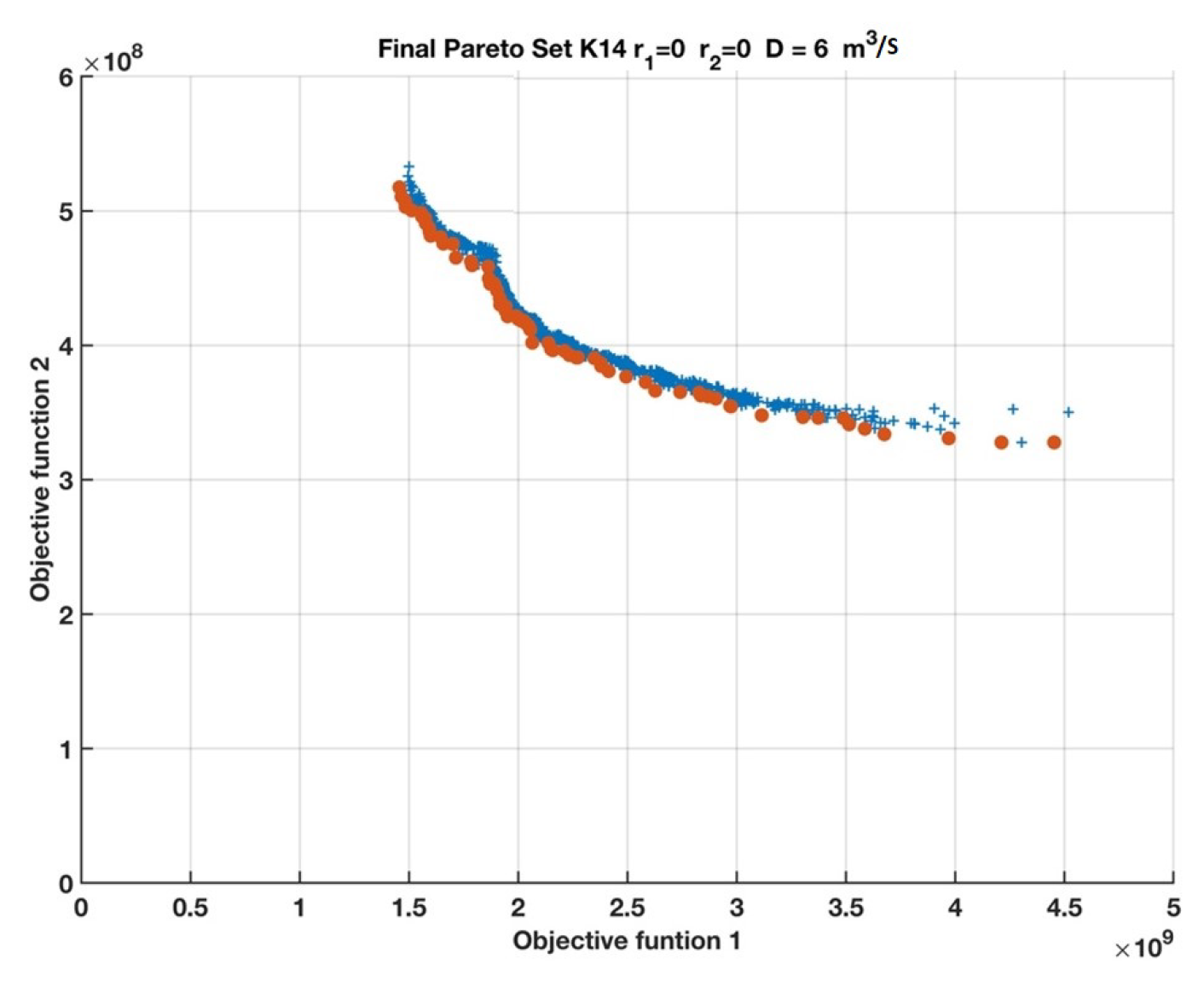
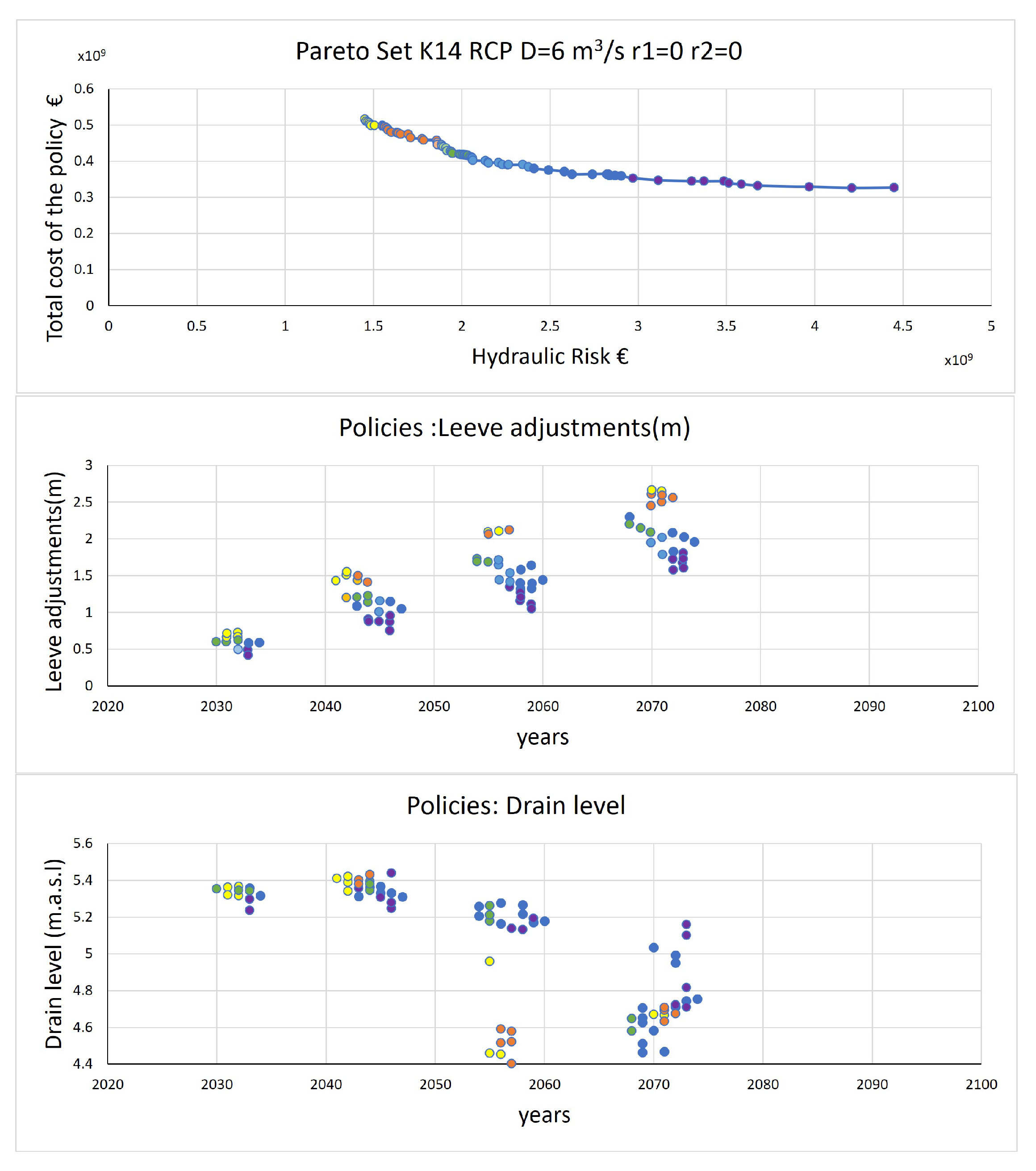
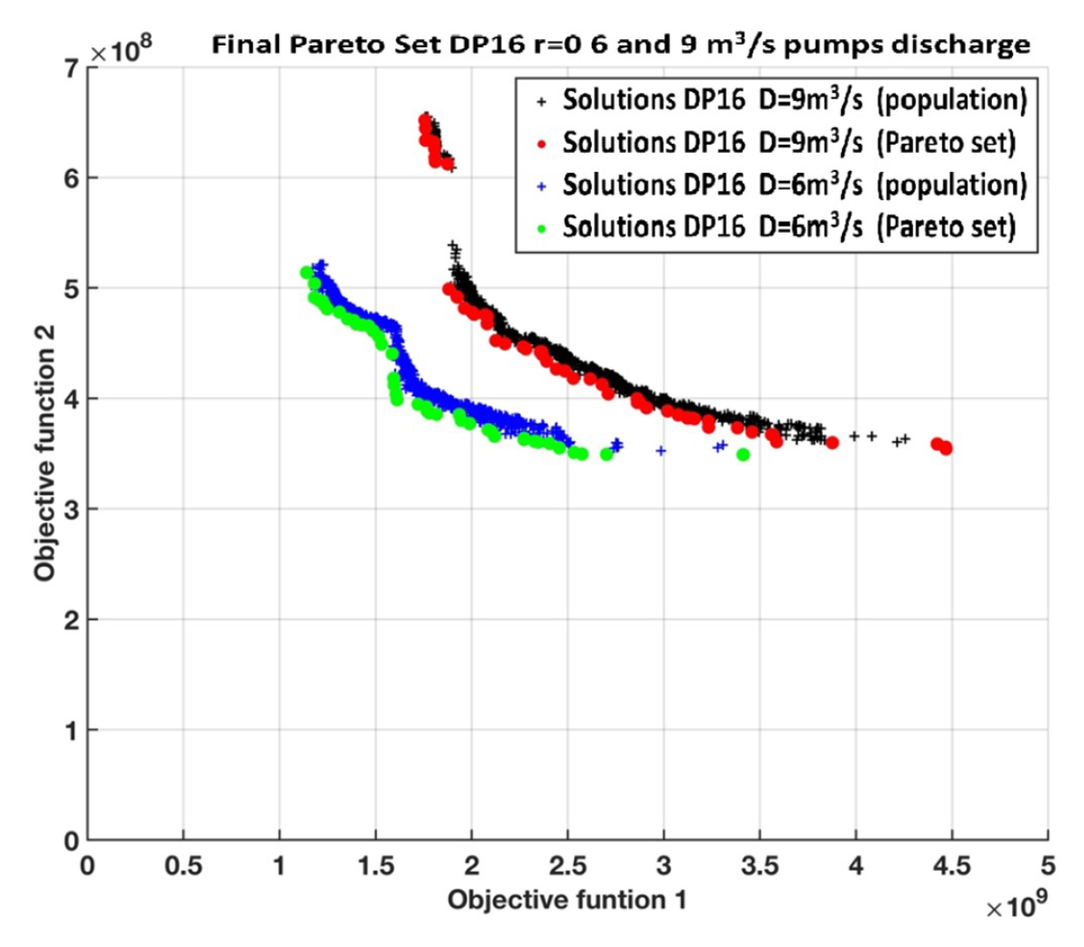
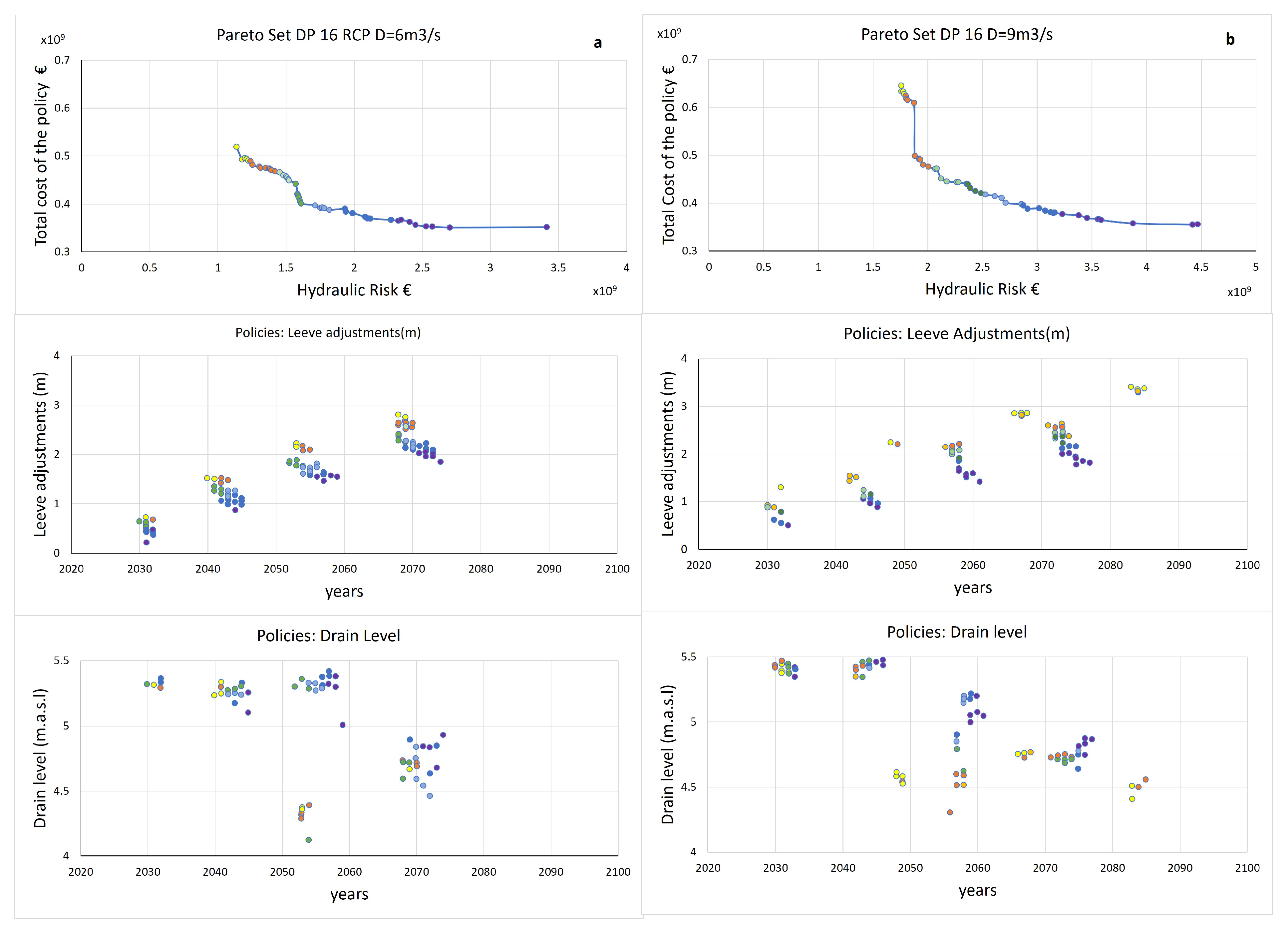
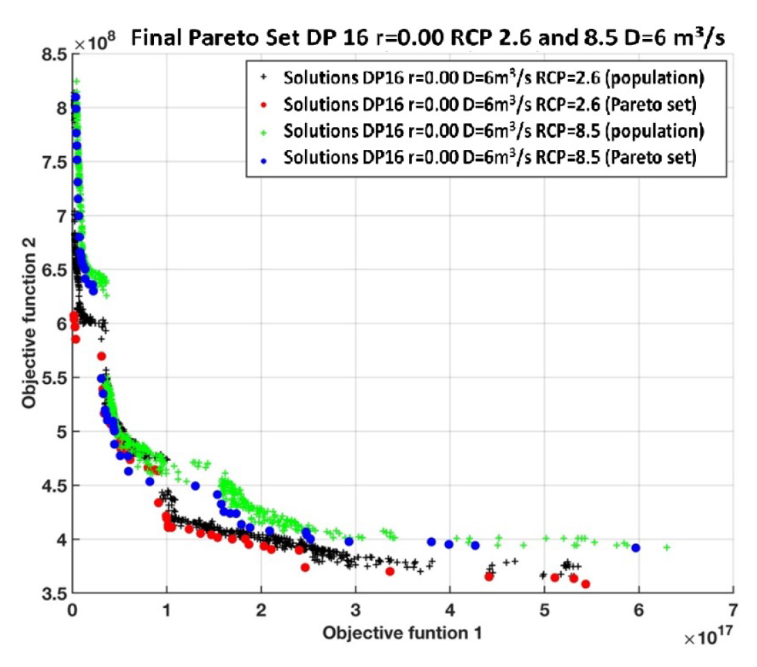
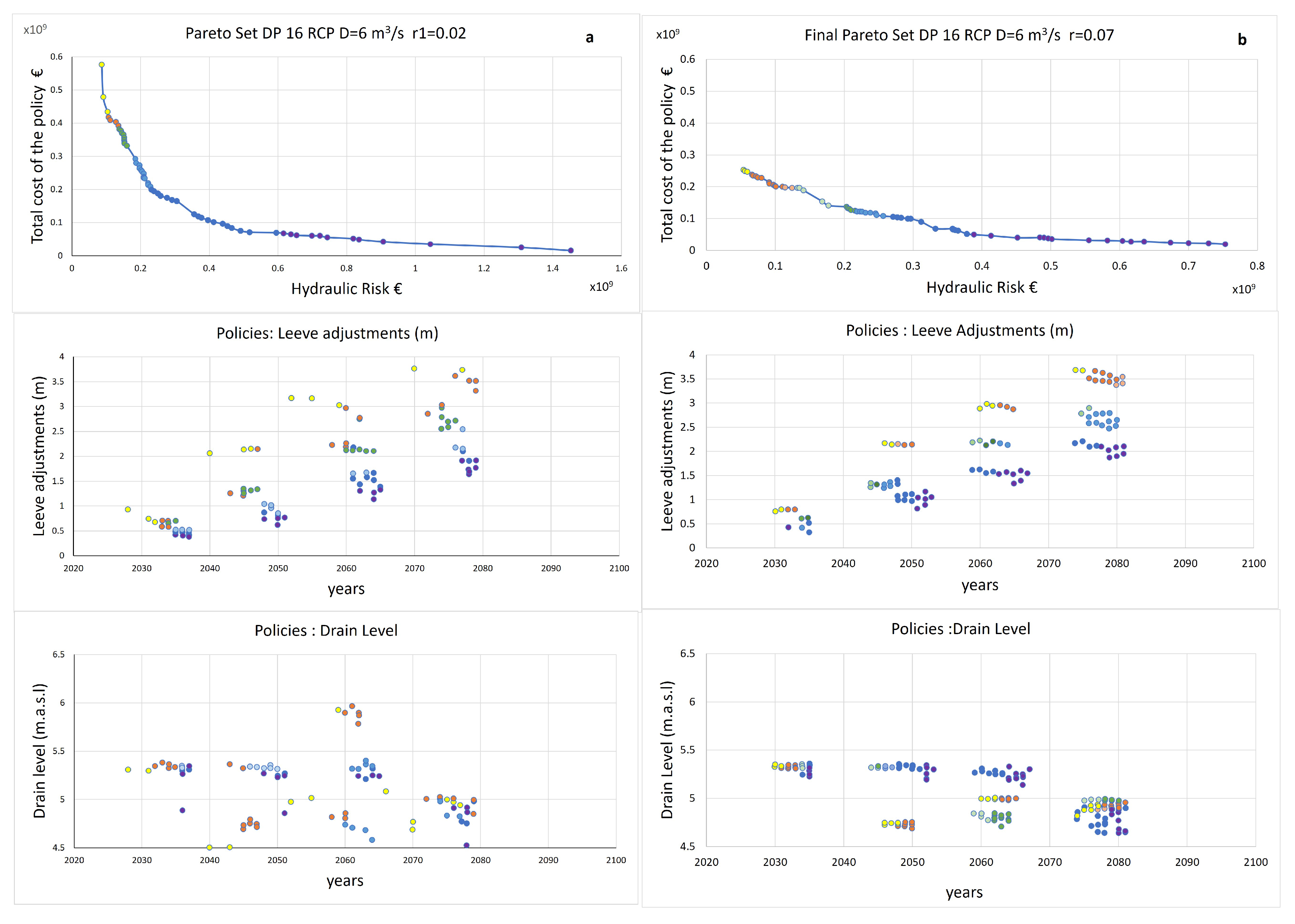
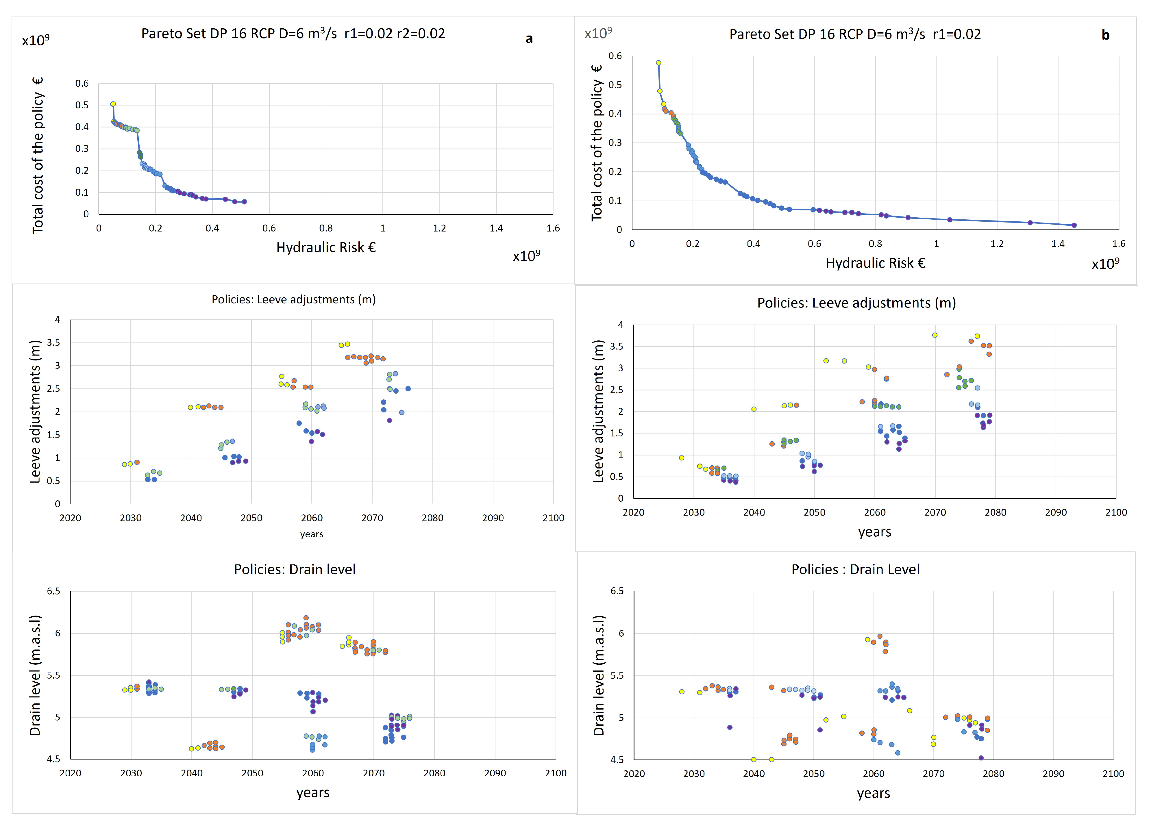
4.4. Application of Multi-Objective Optimization to Case Study

In order to test the reliability of the multiobjective optimization model for identifying the sizing and the timing of the flood defence constructions, five scenarios with different environmental and economic characteristics were taken into into account. These scenarios are listed in the

Table 2. Scenarios description.

	RCPs Considered	Mean Sea Level 2100 Projection	Discount Rate Costs	Discount Rate Damages	Pumping Rate for Each Pump	Selcella Basin’s Damages Accounted
Scenario 1	8.5-4.5-2.6	K14	0	0	6 m3/s	yes
Scenario 2	8.5-4.5-2.6	D16	0	0	6–9 m3/s	yes
Scenario 3	8.5-2.6	D16	0	0	6 m3/s	no
Scenario 4	8.5-4.5-2.6	D16	0.02-0.05-0.07	0	6 m3/s	yes
Scenario 5	8.5-4.5-2.6	D16	0.02	0.02-0.07	6 m3/s	yes

. Scenarios refer to: (a) two sea level rise projections previously discussed capitol k14 and D16; (b) different power of the Mazzocchio pumping station; (c) two different spatial domains to calculate the objective function of Equation (1), the one that takes into account both the areas upstream and downstream from the Mazzocchio pumping station and the one that takes into account only the downstream area; (d) different values of the discount rates $r_d$ and $r_c$. For each of the scenarios considered, Pareto optimal curves were calculated. Each point of Pareto curves identifies the values of decision variables, i.e., the sizing of the flood defence construction and timing.

In the NSGA II algorithm a crowded comparison approach by [47] is used to assure the convergence to the optimal Pareto set and a good spread of solutions. Such approach does not require any user-defined parameter for maintaining diversity among population members. Generally, the algorithm terminates when either a maximum number of generations has been produced, or a satisfactory fitness level has been reached for the population. By performing preliminary runs we selected the minimum number of generations needed to converge to the optimal Pareto set that are reported in

Table 3. NSGA 2 Parameters.

	NSGA II Parameters
Generations	50
Population	1000
Crossover percentage	0.7
Mutation percentage	0.4
Mutation rate	0.02

. In carrying out the multiobjective optimization, 50 generations of 1000 individuals each were assumed. The Table 2 shows the parameters used in the multi-objective optimization algorithm.

The Pareto set obtained solving the multiobjective optimization problem for the scenario 1 of Table 1 is shown in Figure 11. The Pareto curve identifies a set of optimal solutions representing the “best” choices relative to the two objective functions. The curve shows a clear upward concavity: higher costs of flood defence construction reduce the hydraulic risk for the entire period.Each optimal solution belonging to the Pareto set (filled circles) includes the decision variables: size of flood defence works (embankment level and flood expansion area)and timing of their construction. Figure 12 shows the difference among the optimal solutions of Pareto set in term of values of decision variables.

In Figure 12 we explore optimal policy sets by looking at the differences between the safest and most expensive and the most risky and economic ones. The more expensive solutions are characterized by a higher level of banks and time horizons closer to each other (yellow) than the riskier policies (blue) characterized by milder and more distant interventions over time. The solutions (green), positioned in the “elbow” portion of the Pareto Set, are characterized by height levels of the intermediate banks with respect to the solutions that prefer risk or safety.

The second decision variable, that is the level of the drain, presents solutions characterized by an anticipation over time of the more expensive solutions but little variation in terms of altitude up to 2050; the coincidence of the data is due to the contained rise in the sea level up to that date resulting from the K14 projection. In this case, a lower drain level corresponds to higher costs due to a greater portion of land to be allocated to the expansion area. In Figure 13 the Pareto sets obtained for the scenario 2 of Table 2 are shown. The two curves are obtained for two configurations of Mazzocchio pumping station, single pump power of 6 m${}^3$/s and 9 m${}^3$/s. As evidenced in Section 4.2, the increase in the power of pumps reduces the entity of flooding in the basin upstream of Mazzocchio station but at the same time makes worse the hydraulic risk in downstream areas. As it is evident from Figure 13, due to the low economic values of agriculture production in upstream Mazzocchio region, the reduction of the damages in this part of the watershed does not compensate the increased damages in the portion of watershed downstream due to the higher pumping flowrates from Figure 13, the increase of hydraulic risk (Objective function 1) at parity of construction costs is made evident from the translation of the curve associated to the higher values of pumping rates.

As shown in Figure 14a,b, coherently with the higher weight of damage (Objective function 1) in the watershed downstream from Mazzocchio station, the optimal solutions belonging to the Pareto set for 9 m${}^3$/s are characterized by higher top level of levees and larger flood expansion areas than those for 6 m${}^3$/s. Furthermore, the construction times of the defence works in the first case are delayed with respect to the second one. This result suggests to limit the pumping power of Mazzocchio station at 6 m${}^3$/s, since further increase of the pumping power does not produce significant reduction of hydraulic risk for the entire domain, but it makes worse the hydraulic risk in the downstream portion of such domain.

In Figure 15 the Pareto sets obtained for different sea level rise scenarios, referred to RCP 2.6 and RCP 8.5 respectively, are compared. Even if the RCP 2.6 curve presents lower costs than RCP 8.5 curve at parity of hydraulic risk, as expected, the curves are rather close. This is due to the fact that the trends of SLR for RCP2.6 and RCP 8.5 diverge significantly only starting form the 2060. Despite this, the optimal solutions for the two cases are rather different: for RCP8.5 the levee levels are higher than for RCP 2.6. However, construction timings are rather coincident (see Figure 16a,b).

Thus, the model is able to identify the optimal timing in which to implement the planned intervention. Analyzing Figure 16b, it is possible to observe how the more precautionary policies but also the more expensive ones (yellow) foresee more substantial rises of the embankment summits and closer in time, with a maximum time horizon around 2070. The least expensive policies monetary terms but riskier in terms of potential damage from flooding (blue) envisage lower river embankments more distant time horizon with a maximum time horizon of around 2080. In the scenarios 4 and 5 in Table 2, a local projection of sea level rise more severe one in which the phenomenon of the detachment of large portions of ice from the Antarctic polar cap takes place was considered (DP16). For this projection of sea level rise, in scenario 4 in Table 1, the results obtained by varying the cost discount rate $r_c$—equal to $2\%$, $5\%$ and $7\%$ respectively—were compared. We also assume a damage discount rate equal to zero, i.e., the hydraulic risk does not depend on time. Figure 17a,b shows the Pareto sets relating to such scenario in terms of average sea level rise (DP16) by varying, as said, the discounting of the intervention costs and leaving the actualization of the consequent damages unchanged. The main influence of cost discount rate $r_c$ can be inferred comparing Figure 17a,b: greater the cost discount rate is more delayed the flood construction time horizons are. Indeed defence policies, especially the more expensive ones that involve a greater rise in the level of the levees, tend to be anticipated over time by applying the lower cost discount factor $r_c=0.02$ than policies in which a greater costal discount factor $r_c=0.07$ is applied. This is a consequence of the different way in which the cost are weighted in dependence of construction time horizon.

Figure 18a shows the results of the variation of the social discount rate in the case of the DP16 scenario with $r_c=0.02$ and $r_d=0.02$. Comparing with Figure 18b (same case but with $r_d=0$) we observe that, due to the minor weight of the hydraulic risk in future years, the optimal solutions in the case of $r_d=0.02$ are characterized by flood defence works of minor size with construction horizon times anticipated in respect to the case in which rd is assumed equal to zero.

In conclusion, observing the responses of the model to the variations in the social discount rate, both as regards only the costs of carrying out the works, and as regards the associated damages, we note a tendency to anticipate time horizons for the construction of the defence works DP16. Analogous analysis was conducted also for the projections K14, not shown here since results were substantially similar to those of D16 projections. The results presented are intended to offer a tool that the decision maker can rely on to implement planning based for example on a budget limit or on a long-term goal. The input data can be updated from year to year in order to monitor and, if necessary, modify the chosen policy. This is regardless of the RCP scenario that occurs, as the model considers a total probability for each sea level rise and chooses the optimal policies regardless of the RCP scenario. From the results it is possible to observe the model’s ability to grasp differences in the projections of local sea level rise due to a greater contribution from the melting of the Antarctic ice sheet. This difference in the results for the two different projections indicates the model’s ability to adapt even to sudden and significant events, such as the rapid rise in the average sea level due to the fracturing of part of the polar caps with the consequent introduction of huge quantities of water into the ocean. The model is able to identify the optimal time in which to implement the planned intervention. Another aspect evident from the results is the influence of uncertainty on the solutions, it is clear that for modest marine rises and less affected by uncertainty, in which the difference between the 95th and the 5th percentile is small, the solutions tend to concentrate in some very precise instants of time (K14), while with increasing uncertainty (DP16) also the solutions tend to be more varied both as regards the geometric characteristics and for the temporal horizons of realization.

5. Summary and Conclusions

We developed a methodology and related algorithms aimed to identify the size and timing of flood defence constructions to cope with sea level rise, as well as, extreme rainfall regime modification due to climate change. The methodology considers a multi-objective optimization problem. The first objective function is related to the hydraulic risk for the entire climate projection period, while the second one refers to the construction and maintenance costs. Two relevant aspects of the multi-objective optimization problem deserve to be highlighted. First, since the construction timing is considered as a decision variable the projected trend of climate variables, whether it corresponds to uncertain abrupt or smooth changes or in the case in which natural variability shadows climate trend, can be addressed. Second, EAD integrates in its definition the uncertainties in climate projections considering the different RCPs postulated by climate community and for each of these RPCs the structural, parametric and initial condition model uncertainties in climate projections. The relative likelihood of each RCP can be specified by the decision maker, including its possible variation in the future. This way optimism or pessimism as to the ability to mitigate future climate risk can be incorporated. The application to the study case has shown the reliability of the proposed approach which has allowed the identification under different forcing factors of a set of optimal solutions belonging to the Pareto Curve, each of them defining sizing and timing of the flood defence constructions along the entire period of climate projections. There are several areas of potential improvement with future research. First we focused our study just on the flooding over the considered coastal region due to the concomitant action of heavy rainfall, storm surge and sea level rise (SLR) for different global warming scenarios. The SLR also has other impacts on coastal regions which can be equally significant. For instance, coastal erosion that threatens the stability of the shore and dune-coastal lake systems, salt intrusion in coastal aquifers, alteration of ecosystem equilibrium as marshes, or lagoons. Further optimality criteria can be added to the proposed multi-objective optimization scheme without loss of generality. These criteria are not necessarily in monetary terms, since the multi-objective optimization problem can be formulated using incommensurable objectives. In the case study we assumed as flood defences only levees and expansion areas controlled by weirs. Different coastal strategies and policies could be hypothesized to cope sea level rise within the three different categories usually considered and referred as retreat, accommodate and protect [72]. More work needs to be done to assess damages due flooding by hydraulic model simulations to capture the entire landscape of possible options also using water quality or eutrophication models [73], groundwater models [74] or coastal erosion models [75]. A further relevant research suggestion is that proposed by [76], who advocates addressing the unintended negative or positive effects of disaster risk reduction measures and strategies on drought risk. To better design disaster risk reduction (DRR) measures and strategies, it is important to consider interactions between flood and drought which are closely linked hydrological phenomena. The mutual interaction of disaster risk reduction (DRR) measures and strategies aimed to cope the two hydrological risk should be investigated and then formalized within the objective functions. Finally, the proposed approach provides an adaptive and flexible way moving forward the temporal window and then time updating climate projections resulting from future improved GCMs. An ideal application would be as part of an adaptive process where the analysis is updated, for instance, every 5 years with new information and assumptions reflecting the evolution of the climate as well as socio-economic systems, and policy variables such as the discount rate.

References

1. Aerts, J.C.; Botzen, W.W.; Emanuel, K.; Lin, N.; De Moel, H.; Michel-Kerjan, E.O. Evaluating flood resilience strategies for coastal megacities. Science 2014, 344, 473–475. [Google Scholar] [CrossRef] [PubMed]
2. Kron, W. Coasts: The high-risk areas of the world. Nat. Hazards 2013, 66, 1363–1382. [Google Scholar] [CrossRef]
3. Merkens, J.L.; Lincke, D.; Hinkel, J.; Brown, S.; Vafeidis, A.T. Regionalisation of population growth projections in coastal exposure analysis. Clim. Chang. 2018, 151, 413–426. [Google Scholar] [CrossRef] [Green Version]
4. Giorgi, F.; Raffaele, F.; Coppola, E. The response of precipitation characteristics to global warming from climate projections. Earth Syst. Dyn. 2019, 10, 73–89. [Google Scholar] [CrossRef] [Green Version]
5. Lavell, A.; Oppenheimer, M.; Diop, C.; Hess, J.; Lempert, R.; Li, J.; Myeong, S. Managing the risks of extreme events and disasters to advance climate change adaptation. In A Special Report of Working Groups I and II of the Intergovernmental Panel on Climate Change (IPCC); Cambridge University Press: Cambridge, UK, 2012; pp. 25–64. [Google Scholar]
6. Kundzewicz, Z.W.; Kanae, S.; Seneviratne, S.I.; Handmer, J.; Nicholls, N.; Peduzzi, P.; Mechler, R.; Bouwer, L.M.; Arnell, N.; Mach, K.; et al. Flood risk and climate change: Global and regional perspectives. Hydrol. Sci. J. 2014, 59, 1–28. [Google Scholar] [CrossRef] [Green Version]
7. Milly, P.C.; Betancourt, J.; Falkenmark, M.; Hirsch, R.M.; Kundzewicz, Z.W.; Lettenmaier, D.P.; Stouffer, R.J. Stationarity is dead: Whither water management? Science 2008, 319, 573–574. [Google Scholar] [CrossRef] [PubMed]
8. Doss-Gollin, J.; Farnham, D.J.; Steinschneider, S.; Lall, U. Robust adaptation to multiscale climate variability. Earth Future 2019, 7, 734–747. [Google Scholar] [CrossRef] [Green Version]
9. Van Vuuren, D.P.; Edmonds, J.; Kainuma, M.; Riahi, K.; Thomson, A.; Hibbard, K.; Hurtt, G.C.; Kram, T.; Krey, V.; Lamarque, J.F.; et al. The representative concentration pathways: An overview. Clim. Chang. 2011, 109, 5–31. [Google Scholar] [CrossRef]
10. Parker, W.S. Predicting weather and climate: Uncertainty, ensembles and probability. Stud. Hist. Philos. Sci. Part B Stud. Hist. Philos. Mod. Phys. 2010, 41, 263–272. [Google Scholar] [CrossRef]
11. Holt, J.; Harle, J.; Proctor, R.; Michel, S.; Ashworth, M.; Batstone, C.; Allen, I.; Holmes, R.; Smyth, T.; Haines, K.; et al. Modelling the global coastal ocean. Philos. Trans. R. Soc. A Math. Phys. Eng. Sci. 2009, 367, 939–951. [Google Scholar] [CrossRef] [Green Version]
12. Penduff, T.; Juza, M.; Barnier, B.; Zika, J.; Dewar, W.K.; Treguier, A.M.; Molines, J.M.; Audiffren, N. Sea level expression of intrinsic and forced ocean variabilities at interannual time scales. J. Clim. 2011, 24, 5652–5670. [Google Scholar] [CrossRef]
13. Little, C.M.; Urban, N.M. CMIP5 temperature biases and 21st century warming around the Antarctic coast. Ann. Glaciol. 2016, 57, 69–78. [Google Scholar] [CrossRef] [Green Version]
14. Cioffi, F.; Conticello, F.; Lall, U.; Marotta, L.; Telesca, V. Large scale climate and rainfall seasonality in a Mediterranean Area: Insights from a non-homogeneous Markov model applied to the Agro-Pontino plain. Hydrol. Process. 2017, 31, 668–686. [Google Scholar] [CrossRef]
15. Conticello, F.; Cioffi, F.; Merz, B.; Lall, U. An event synchronization method to link heavy rainfall events and large-scale atmospheric circulation features. Int. J. Climatol. 2018, 38, 1421–1437. [Google Scholar] [CrossRef]
16. Orton, P.; Conticello, F.; Cioffi, F.; Hall, T.; Georgas, N.; Lall, U.; Blumberg, A.; MacManus, K. Flood hazard assessment from storm tides, rain and sea level rise for a tidal river estuary. Nat. Hazards 2020, 102, 729–757. [Google Scholar] [CrossRef]
17. Tebaldi, C.; Friedlingstein, P. Delayed detection of climate mitigation benefits due to climate inertia and variability. Proc. Natl. Acad. Sci. USA 2013, 110, 17229–17234. [Google Scholar] [CrossRef] [Green Version]
18. Kopp, R.E.; Horton, R.M.; Little, C.M.; Mitrovica, J.X.; Oppenheimer, M.; Rasmussen, D.; Strauss, B.H.; Tebaldi, C. Probabilistic 21st and 22nd century sea-level projections at a global network of tide-gauge sites. Earth Future 2014, 2, 383–406. [Google Scholar] [CrossRef]
19. Balica, S.F.; Wright, N.G.; Van der Meulen, F. A flood vulnerability index for coastal cities and its use in assessing climate change impacts. Nat. Hazards 2012, 64, 73–105. [Google Scholar] [CrossRef] [Green Version]
20. Muis, S.; Güneralp, B.; Jongman, B.; Aerts, J.C.; Ward, P.J. Flood risk and adaptation strategies under climate change and urban expansion: A probabilistic analysis using global data. Sci. Total. Environ. 2015, 538, 445–457. [Google Scholar] [CrossRef]
21. Ramieri, E.; Hartley, A.; Barbanti, A.; Santos, F.D.; Gomes, A.; Hilden, M.; Laihonen, P.; Marinova, N.; Santini, M. Methods for assessing coastal vulnerability to climate change. ETC CCA Tech. Pap. 2011, 1, 1–93. [Google Scholar]
22. van der Sluijs, J.P.; Dessai, S. Uncertainty and Climate Change Adaptation—A Scoping Study; Copernicus Institute for Sustainable Development and Innovation: Utrecht, The Netherlands, 2007. [Google Scholar]
23. Kwadijk, J.C.; Haasnoot, M.; Mulder, J.P.; Hoogvliet, M.M.; Jeuken, A.B.; van der Krogt, R.A.; van Oostrom, N.G.; Schelfhout, H.A.; van Velzen, E.H.; van Waveren, H.; et al. Using adaptation tipping points to prepare for climate change and sea level rise: A case study in the Netherlands. Wiley Interdiscip. Rev. Clim. Chang. 2010, 1, 729–740. [Google Scholar] [CrossRef]
24. Haasnoot, M.; Kwakkel, J.H.; Walker, W.E.; Ter Maat, J. Dynamic adaptive policy pathways: A method for crafting robust decisions for a deeply uncertain world. Glob. Environ. Chang. 2013, 23, 485–498. [Google Scholar] [CrossRef] [Green Version]
25. Walker, W.E.; Rahman, S.A.; Cave, J. Adaptive policies, policy analysis, and policy-making. Eur. J. Oper. Res. 2001, 128, 282–289. [Google Scholar] [CrossRef] [Green Version]
26. Kwakkel, J.; Haasnoot, M. Computer Assisted Dynamic Adaptive Policy Design for Sustainable Water Management in River Deltas in a Changing Environment; Brigham Young University: Provo, UT, USA, 2012. [Google Scholar]
27. Parry, M.L.; Canziani, O.; Palutikof, J.; Van der Linden, P.; Hanson, C. Climate Change 2007-Impacts, Adaptation and Vulnerability: Working Group II Contribution to the Fourth Assessment Report of the IPCC; Cambridge University Press: Cambridge, UK, 2007; Volume 4. [Google Scholar]
28. Löwe, R.; Urich, C.; Domingo, N.S.; Mark, O.; Deletic, A.; Arnbjerg-Nielsen, K. Assessment of urban pluvial flood risk and efficiency of adaptation options through simulations—A new generation of urban planning tools. J. Hydrol. 2017, 550, 355–367. [Google Scholar] [CrossRef] [Green Version]
29. Woodward, M.; Kapelan, Z.; Gouldby, B. Adaptive flood risk management under climate change uncertainty using real options and optimization. Risk Anal. 2014, 34, 75–92. [Google Scholar] [CrossRef]
30. Lenton, T.M.; Rockström, J.; Gaffney, O.; Rahmstorf, S.; Richardson, K.; Steffen, W.; Schellnhuber, H.J. Climate tipping points too risky to bet against. Nature 2020, 575, 592–595. [Google Scholar] [CrossRef]
31. Cioffi, F.; Gallerano, F. Multi-objective analysis of dam release flows in rivers downstream from hydropower reservoirs. Appl. Math. Model. 2012, 36, 2868–2889. [Google Scholar] [CrossRef] [Green Version]
32. Ngatchou, P.; Zarei, A.; El-Sharkawi, A. Pareto multi objective optimization. In Proceedings of the 13th International Conference on, Intelligent Systems Application to Power Systems, Arlington, VA, USA, 6–10 November 2005; pp. 84–91. [Google Scholar]
33. Arnell, N.W. Expected annual damages and uncertainties in flood frequency estimation. J. Water Resour. Plan. Manag. 1989, 115, 94–107. [Google Scholar] [CrossRef] [Green Version]
34. Deb, K.; Thiele, L.; Laumanns, M.; Zitzler, E. Scalable multi-objective optimization test problems. In Proceedings of the 2002 Congress on Evolutionary Computation—CEC’02 (Cat. No. 02TH8600), Honolulu, HI, USA, 12–17 May 2002; Volume 1, pp. 825–830. [Google Scholar]
35. Nazarnia, H.; Nazarnia, M.; Sarmasti, H.; Wills, W.O. A systematic review of civil and environmental infrastructures for coastal adaptation to sea level rise. Civ. Eng. J. 2020, 6, 1375–1399. [Google Scholar] [CrossRef]
36. Winsemius, H.; Van Beek, L.; Jongman, B.; Ward, P.; Bouwman, A. A framework for global river flood risk assessments. Hydrol. Earth Syst. Sci. 2013, 17, 1871–1892. [Google Scholar] [CrossRef] [Green Version]
37. Coles, S.G.; Tawn, J.A. Modelling extreme multivariate events. J. R. Stat. Soc. Ser. B Methodol. 1991, 53, 377–392. [Google Scholar] [CrossRef]
38. Johnson, L.T.; Hope, C. The social cost of carbon in US regulatory impact analyses: An introduction and critique. J. Environ. Stud. Sci. 2012, 2, 205–221. [Google Scholar] [CrossRef]
39. Gollier, C.; Hammitt, J.K. The long-run discount rate controversy. Annu. Rev. Resour. Econ. 2014, 6, 273–295. [Google Scholar] [CrossRef] [Green Version]
40. Jonkman, S.N.; Bočkarjova, M.; Kok, M.; Bernardini, P. Integrated hydrodynamic and economic modelling of flood damage in the Netherlands. Ecol. Econ. 2008, 66, 77–90. [Google Scholar] [CrossRef]
41. Bossard, M.; Feranec, J.; Otahel, J. CORINE Land Cover Technical Guide: Addendum 2000; European Environment Agency Copenhagen: København, Denmark, 2000; Volume 40. [Google Scholar]
42. Scawthorn, C.; Flores, P.; Blais, N.; Seligson, H.; Tate, E.; Chang, S.; Mifflin, E.; Thomas, W.; Murphy, J.; Jones, C.; et al. HAZUS-MH Flood loss estimation methodology. II: Damage and loss assessment. Nat. Hazards Rev. 2006, 7, 72–81. [Google Scholar] [CrossRef]
43. HAZUS-MH Flood. Flood Model: Technical Manual; Federal Emergency Management Agency: Washington, DC, USA, 2003.
44. Riddell, K.; Green, C. Flood and coastal defence project appraisal guidance: Economic appraisal. In FDCPAG3; Ministry of Agriculture, Food and Fisheries: Tokyo, Japan, 1999. [Google Scholar]
45. Cioffi, F.; De Bonis Trapella, A.; Conticello, F.R. Efficiency assessment of existing pumping/hydraulic network systems to mitigate flooding in low-lying coastal regions under different scenarios of sea level rise: The Mazzocchio area study case. Water 2018, 10, 820. [Google Scholar] [CrossRef] [Green Version]
46. Jonkman, S.N.; Hillen, M.M.; Nicholls, R.J.; Kanning, W.; van Ledden, M. Costs of adapting coastal defences to sea-level rise—New estimates and their implications. J. Coast. Res. 2013, 29, 1212–1226. [Google Scholar] [CrossRef]
47. Deb, K.; Pratap, A.; Agarwal, S.; Meyarivan, T. A fast and elitist multiobjective genetic algorithm: NSGA-II. IEEE Trans. Evol. Comput. 2002, 6, 182–197. [Google Scholar] [CrossRef] [Green Version]
48. Goldberg, D.E.; Deb, K. A comparative analysis of selection schemes used in genetic algorithms. In Foundations of Genetic Algorithms; Elsevier: Amsterdam, The Netherlands, 1991; Volume 1, pp. 69–93. [Google Scholar]
49. Deb, K.; Agrawal, R.B. Simulated binary crossover for continuous search space. Complex Syst. 1995, 9, 115–148. [Google Scholar]
50. Kemp, A.C.; Horton, B.P.; Donnelly, J.P.; Mann, M.E.; Vermeer, M.; Rahmstorf, S. Climate related sea-level variations over the past two millennia. Proc. Natl. Acad. Sci. USA 2011, 108, 11017–11022. [Google Scholar] [CrossRef] [PubMed] [Green Version]
51. Vermeer, M.; Rahmstorf, S. Global sea level linked to global temperature. Proc. Natl. Acad. Sci. USA 2009, 106, 21527–21532. [Google Scholar] [CrossRef] [PubMed] [Green Version]
52. Lian, J.; Xu, K.; Ma, C. Joint impact of rainfall and tidal level on flood risk in a coastal city with a complex river network: A case study of Fuzhou City, China. Hydrol. Earth Syst. Sci. 2013, 17, 679–689. [Google Scholar] [CrossRef] [Green Version]
53. Coles, S.; Heffernan, J.; Tawn, J. Dependence measures for extreme value analyses. Extremes 1999, 2, 339–365. [Google Scholar] [CrossRef]
54. Zheng, F.; Westra, S.; Leonard, M.; Sisson, S.A. Modeling dependence between extreme rainfall and storm surge to estimate coastal flooding risk. Water Resour. Res. 2014, 50, 2050–2071. [Google Scholar] [CrossRef]
55. De Haan, L. A spectral representation for max-stable processes. Ann. Probab. 1984, 12, 1194–1204. [Google Scholar]
56. Kopp, R.E.; DeConto, R.M.; Bader, D.A.; Hay, C.C.; Horton, R.M.; Kulp, S.; Oppenheimer, M.; Pollard, D.; Strauss, B.H. Evolving understanding of Antarctic ice-sheet physics and ambiguity in probabilistic sea-level projections. Earth Future 2017, 5, 1217–1233. [Google Scholar] [CrossRef] [Green Version]
57. DeConto, R.M.; Pollard, D. Contribution of Antarctica to past and future sea-level rise. Nature 2016, 531, 591–597. [Google Scholar] [CrossRef]
58. Milne, G.; Gehrels, W.; Hughes, C.; Tamisiea, M. Identifying the causes of sea-level change. Nat. Geosci. 2009, 2, 471–478. [Google Scholar] [CrossRef] [Green Version]
59. Taylor, K.E.; Stouffer, R.J.; Meehl, G.A. An overview of CMIP5 and the experiment design. Bull. Am. Meteorol. Soc. 2012, 93, 485–498. [Google Scholar] [CrossRef] [Green Version]
60. Rahmstorf, S.; Perrette, M.; Vermeer, M. Testing the robustness of semi-empirical sea level projections. Clim. Dyn. 2012, 39, 861–875. [Google Scholar] [CrossRef]
61. Kopp, R.E. Does the mid-Atlantic United States sea level acceleration hot spot reflect ocean dynamic variability? Geophys. Res. Lett. 2013, 40, 3981–3985. [Google Scholar] [CrossRef]
62. Bamber, J.L.; Aspinall, W. An expert judgement assessment of future sea level rise from the ice sheets. Nat. Clim. Chang. 2013, 3, 424–427. [Google Scholar] [CrossRef]
63. Marzeion, B.; Jarosch, A.; Hofer, M. Past and future sea-level change from the surface mass balance of glaciers. Cryosphere 2012, 6, 1295–1322. [Google Scholar] [CrossRef] [Green Version]
64. Cioffi, F.; Gallerano, F. Management strategies for the control of eutrophication processes in Fogliano lagoon (Italy): A long-term analysis using a mathematical model. Appl. Math. Model. 2001, 25, 385–426. [Google Scholar] [CrossRef]
65. Kimura, N.; Tai, A.; Chiang, S.; Wei, H.P.; Su, Y.F.; Cheng, C.T.; Kitoh, A. Hydrological flood simulation using a design hyetograph created from extreme weather data of a high-resolution atmospheric general circulation model. Water 2014, 6, 345–366. [Google Scholar] [CrossRef] [Green Version]
66. Berrisford, P.; Dee, D.; Poli, P.; Brugge, R.; Fielding, K.; Fuentes, M.; Kallberg, P.; Kobayashi, S.; Uppala, S.; Simmons, A. The ERA-Interim Archive. Era Rep. Ser. 2011, 1, 1–16. [Google Scholar]
67. Milano, V. Idraulica Marittima; Maggioli Editore: Santarcangelo, Italy, 2008; Volume 152. [Google Scholar]
68. Pawlowicz, R.; Beardsley, B.; Lentz, S. Classical tidal harmonic analysis including error estimates in MATLAB using T_TIDE. Comput. Geosci. 2002, 28, 929–937. [Google Scholar] [CrossRef]
69. Scotti, V.; Giannini, M.; Cioffi, F. Enhanced flood mapping using synthetic aperture radar (SAR) images, hydraulic modelling, and social media: A case study of Hurricane Harvey (Houston, TX). J. Flood Risk Manag. 2020, 13, e12647. [Google Scholar] [CrossRef]
70. Farhadi, H.; Najafzadeh, M. Flood Risk Mapping by Remote Sensing Data and Random Forest Technique. Water 2021, 13, 3115. [Google Scholar] [CrossRef]
71. Farhadi, H.; Esmaeily, A.; Najafzadeh, M. Flood monitoring by integration of Remote Sensing technique and Multi-Criteria Decision Making method. Comput. Geosci. 2022, 160, 105045. [Google Scholar] [CrossRef]
72. Doberstein, B.; Fitzgibbons, J.; Mitchell, C. Protect, accommodate, retreat or avoid (PARA): Canadian community options for flood disaster risk reduction and flood resilience. Nat. Hazards 2019, 98, 31–50. [Google Scholar] [CrossRef]
73. Cioffi, F.; Gallerano, F. From rooted to floating vegetal species in lagoons as a consequence of the increases of external nutrient load: An analysis by model of the species selection mechanism. Appl. Math. Model. 2006, 30, 10–37. [Google Scholar] [CrossRef] [Green Version]
74. Giambastiani, B.M.; Antonellini, M.; Essink, G.H.O.; Stuurman, R.J. Saltwater intrusion in the unconfined coastal aquifer of Ravenna (Italy): A numerical model. J. Hydrol. 2007, 340, 91–104. [Google Scholar] [CrossRef]
75. Gallerano, F.; Cannata, G.; De Gaudenzi, O.; Scarpone, S. Modeling bed evolution using weakly coupled phase-resolving wave model and wave-averaged sediment transport model. Coast. Eng. J. 2016, 58, 1650011. [Google Scholar] [CrossRef] [Green Version]
76. Ward, P.J.; de Ruiter, M.C.; Mård, J.; Schröter, K.; Van Loon, A.; Veldkamp, T.; von Uexkull, N.; Wanders, N.; AghaKouchak, A.; Arnbjerg-Nielsen, K.; et al. The need to integrate flood and drought disaster risk reduction strategies. Water Secur. 2020, 11, 100070. [Google Scholar] [CrossRef]
Figure 1. Uncertainties in climate projection due to (a) future CO2 emission scenarios; [18] (b) uncertainties in climate modelling; (c) long period natural cycle [8].
Water 14 01481 g001
Figure 2. Sketch of model system.
Water 14 01481 g002
Figure 3. Hydraulic network of Pontina Plain with maneuvers, pumping stations and gates.
Water 14 01481 g003
Figure 4. Downscaled projections used to calculate the total probability of sea level rise D16 (top) and K14 (bottom).
Water 14 01481 g004
Figure 5. Sketch of integration domain.
Water 14 01481 g005
Figure 6. Hyetograph (top) and the sea level (Bottom) trend recorded during the event of 25 November 2018 respectively.
Water 14 01481 g006
Figure 7. Comparison between flooding areas by Sentinel 1 satellite image (a) and simulated ones (b).
Water 14 01481 g007
Figure 8. Maximum flow depth difference between configuration with 1.5 increase of pumping flow rate of each single pump (9 m3/s) at Mazzocchio pumping station and the current one (6 m3/s).
Water 14 01481 g008
Figure 9. (ad) Comparison of the water depth field at the instant of maximum flooding for the current average sea level and that assuming an average sea level rise equal to m. 0.5.
Water 14 01481 g009
Figure 10. Probability density functions at the year 2050 and 2100 for each RCPs, for the sea level rise scenario K14 (a) and Dp16 (b) respectively.
Water 14 01481 g010
Figure 11. Pareto set for scenario 1. of Table 2.
Water 14 01481 g011
Figure 12. Size and timing of Flood defence constructions for the Pareto set optimal solutions.
Water 14 01481 g012
Figure 13. Pareto set for scenario 2 of Table 2.
Water 14 01481 g013
Figure 14. (a,b) Size and timing of Flood defence constructions for the Pareto set optimal solutions referred to scenario 2 of Table 2.
Water 14 01481 g014
Figure 15. Pareto set for scenario 3 of Table 2.
Water 14 01481 g015
Figure 16. (a,b) Size and timing of Flood defence constructions for the Pareto set optimal solutions referred to scenario 3 of Table 2.
Water 14 01481 g016
Figure 17. (a,b) Size and timing of Flood defence constructions for the Pareto set optimal solutions referred to scenario 4 of Table 1.
Water 14 01481 g017
Figure 18. (a,b) Size and timing of Flood defence constructions for the Pareto set optimal solutions referred to scenario 5 of Table 1.
Water 14 01481 g018