Detection and Quantification of Dam Leakages Based on Tracer Tests: A Field Case Study

Abstract

Leakage is a common phenomenon in dams, and its early detection is critical for dam safety. In the present study, a new method based on tracer tests is applied to detect and quantify leakage in the Wanyao Dam, Jiangshan City, China. The objective is to detect the leakage zone of a dam wall by combining the natural tracer test and the artificial tracer test. Temperature, electrical well-logging tests with nature tracers, and the artificial tracer test with salt (NaCl) were conducted using 48 and 5 pre-existing boreholes, respectively. Using natural tracer tests, the 48 boreholes are categorized into 4 leakage classes: (1) Class 1, high connectivity within whole borehole; (2) Class 2 high connectivity at lower depths; (3) Class 3, weaken connectivity; and (4) Class 4, safe boreholes with no connectivity. Using the proposed method, specific leakage rates of some boreholes were estimated. The results of the new method are validated by comparison with those from natural tracer tests, site-investigation, and historical observation data. Overall, the new tracer test has the following merits: (1) low cost, (2) environment friendliness, and (3) is simple to apply. Moreover, the proposed method improves the accuracy of traditional tracer tests for detecting leakage zones.

1. Introduction

Up to March 2011, the Global Reservoir and Dam Database collected information on 6862 dams and the associated reservoirs with a total storage capacity of 6197 km³ [1]. Leakage is of paramount importance for the safe operation of dams and reservoirs. In hydraulic engineering, leakage is a common phenomenon in dams, which is even considered in the design stage. However, it is difficult and uneconomical to eliminate all potential leakage problems in the engineering design of hydraulic structures such as dams. Yet, even small leakages can develop into erosion and fractures, which may eventually threaten the structural stability of dams. Hence, the early detection and estimation of leakage are critical in facilitating the repair of the leakage zone to ensure safe dam operation.

Geophysical methods such as electrical resistivity tomography, seismic tomography, and ground penetrating radar are commonly used for detecting and locating leakage zones in dams. For example, Ikard et al. [2] and Minsley et al. [3] used the resistivity method and self-potential tomography to investigate seepage in earth dams. Demanet and Jongmans [4] applied seismic tomography to locate the fracture zone while Di Prinzio et al. [5] and Xu et al., [6] used ground penetrating radar to detect voids in river embankments or dams. Al-Fares [7] used superficial electromagnetic, electrical sounding, and electrical resistivity tomography to characterize water leakage in dams. Similarly, Bièvre et al. [8] used electrical resistivity tomography (ERT) to characterize leakage. These approaches estimated the spatial heterogeneity in embankments based on contrasts of physical parameters of different media. Geophysical methods have the advantages of giving high resolution data and are non-destructive. However, these geophysical methods often need expensive equipment, expertise, and complex computation and interpretation algorithms. Moreover, these methods provide indirect evidence based on physical indices reflecting the permeability of earth materials or concrete rather than quantifying the seepage or groundwater flow. Therefore, it is difficult to accurately quantify leakage using geophysical methods.

Compared to geophysical methods, tracer tests have a number of advantages, including low-cost, high efficiency, and provide direct data on the seepage or groundwater flow field. Tracer tests have been used for detecting dam leakages for more than 40 years [9]. Basically, tracers can be classified into natural and artificial tracers. Natural tracers are based on inherent physical or chemical characteristics of the fluid, such as temperature, electrical conductivity (EC), total dissolved solids, and stable isotopes. Temperature, EC, and total dissolved solids are parameters that can be measured easily in situ using a probe attached to a cable. The convenient and low-cost measurement of natural tracers provides geoscientists with an easy method to investigate the source of leakage [10,11,12,13]. The artificial tracers include salt, radioactive isotopes, and dyes (e.g., fluorescein) [13,14,15,16]. Based on the injection of an artificial tracer and subsequent analysis of the data, detailed information on the flow field can be obtained [13,14,15,16,17,18,19,20,21,22]. The common applications of tracers include: (1) calculating flow velocity; (2) confirming the hydraulic connectivity, and (3) estimating relative hydraulic properties based on the concentration curves.

The single borehole dilution test (SBDT) is a type of tracer test using artificial tracers, which is widely used in investigating saturated aquifers. The SBDT is attractive in leakage detection due to its ability to determine seepage velocity. In this regard, SBDT can be used for the following applications: (1) to observe the transport distance of tracers over time between source and receptors [23]; (2) to analyze the distance or amplitude of peak concentration [20,24,25]; and (3) to interpret breakthrough curves based on the convection-dispersion equation [26,27,28,29,30]. SBDT can be applied either as a point injection or uniform injection, but the former is preferred to calculate flow velocity.

The leakage problem in the Wanyao dam poses safety problems, including the malfunctioning of electrical systems. In a previous study using hydrochemical analysis and tracer tests, Huang et al. [21] confirmed the hydraulic connectivity between leakage inside the dam wall and the reservoir and speculated that a leakage path existed inside the dam. However, the earlier study by Huang et al. [21] did not address the following: (1) quantifying the seepage in the different sections of the dam wall; and (2) identifying and characterizing the seepage or fracture zone with the leakage phenomenon. The present study seeks to address these aspects, and a network of standardized observation boreholes inside the dam wall makes this possible using natural and artificial tracer tests.

A review of earlier literature shows that few studies have investigated the use of the SBDT to detect and quantify leakage of hydraulic engineering structures such as dams. The only available studies are limited to the application of SBDT to aquifers [23,28,29,31]. Therefore, in the current paper, an improved method based on the tracer test is developed and applied to detect and estimate leakage from a dam wall. The method applies the concept of squeeze theorem in mathematics [32], and the law of Conservation of Mass in physics. The objectives of this study are to: (1) detect the leakage zone in the dam wall; (2) make qualitative and quantitative analysis of leakage rates by applying the natural tracer test and the new approach based on SBDT; (3) test the limitations and accuracy of the new approach. This present study is a typical case for locating leakage paths and calculating the flow rate with the tracer test after the source of leakage is determined.

2. Theoretical Background

2.1. Natural Tracer

The present study uses temperature and EC, which are used as common natural tracers of seepage patterns in the dam wall. The rationale is that the depth distributions of water temperature and electric conductivity of weak and slow leakage are more stable and smoother than that of severe and quick seepage. In other words, severe and quick seepage is characterized by rapid or abrupt changes in the depth distribution of water temperature and EC. In hydraulic engineering, slow seepage is acceptable, because it is accounted for in the design stage. If water flows slowly inside the dam, it interacts with, and its hydrochemistry is fully affected by, the surrounding rocks, resulting in a smooth variation in the temperature field. On the contrary, the severe leakage in the dam wall maintains its inherent temperature or hydrochemical properties because of the less contact time and interaction with the surrounding rocks. Hence, the severe leakage often makes obvious and sharp changes in the original temperature or EC field. This difference in temperature or hydrochemical behavior is used by engineers and geoscientists to locate flow paths or zones with high fracture density in hydraulic structures such as dams [10,11,12,13,14,15,16,17,18,19,20].

Thus, similar to temperature, the EC of water is also an index that can represent the degree of interactions between seepage water and the surrounding rocks. The EC of water increases with the contact time and interaction with rocks owing to the release of solutes from rocks, including via acid-based reactions with carbonic acid [33]. Samples with larger EC often have a longer contact time with rocks [10] while those with a low EC indicate a short contact time or interaction with surrounding rocks.

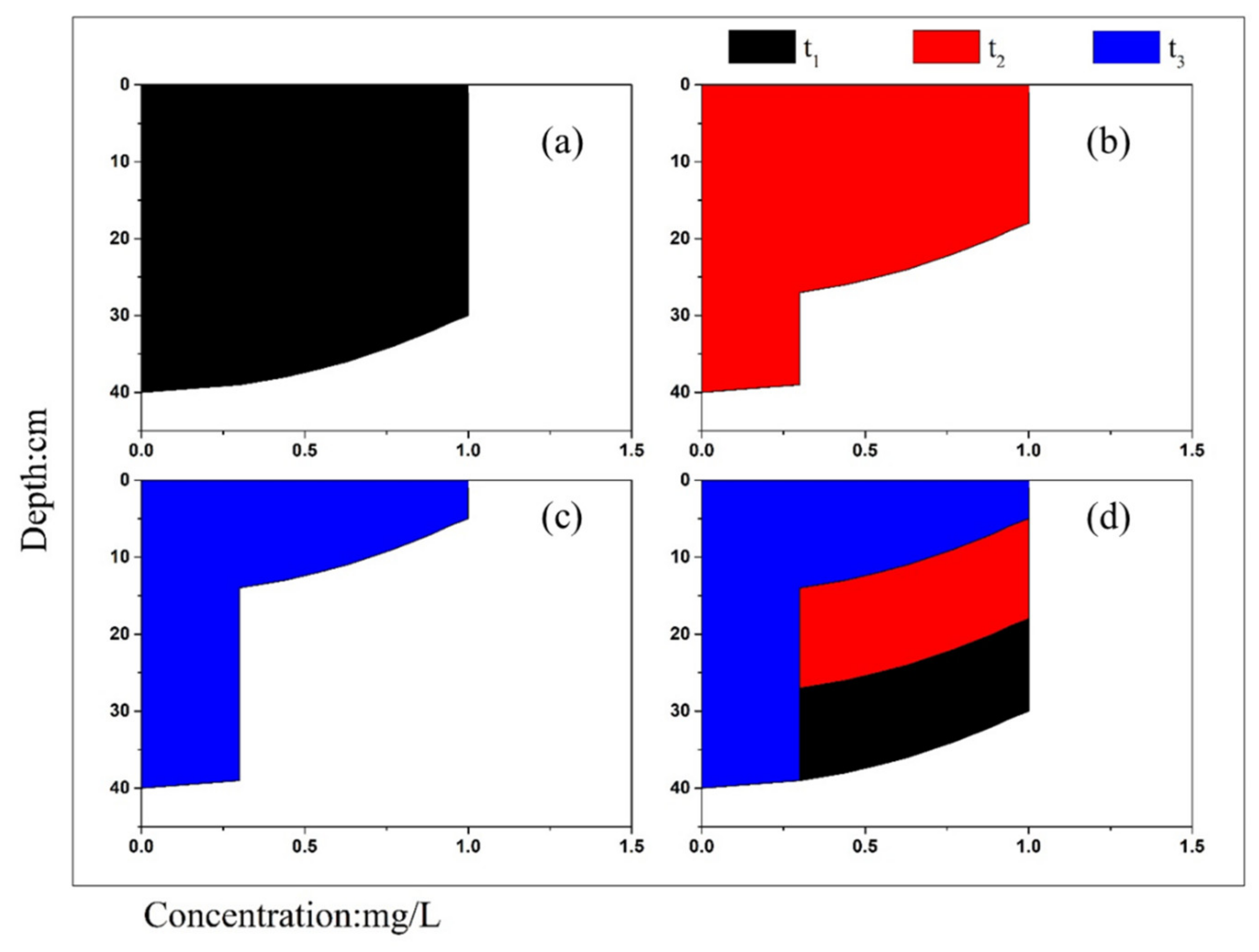
2.2. Singe Borehole Dilution Tests

SBDT characterizes the hydraulic properties and flow field within a depth by analyzing tracer variations during dilution. It is used widely to investigate saturated aquifers due to easy measurement and low-cost. As early as the late 1960s, Walter et al., [34] used the SBDT to compare the hydraulic conductivity of aquifer media. Using the measurement probe and theory discussed earlier, SBDT was utilized to characterize zones with high fracture density, identify ambient flows, estimate flux or flow velocity, and detect leakages or voids in aquifers and fractured rocks [23,26,28,29,30,34,35]. However, limited studies have applied the SBDT method to determine seepage zones and flow rates in hydraulic structures such as dams.

Point and uniform injection methods are the two common types of SBDT. Point injection releases tracer in part of a borehole. By monitoring the movement of the tracer or peak EC concentration of water, the flow velocity (v) can be calculated using Equation (1):

$$v=\frac{\Delta L}{\Delta t},$$

(1)

where $\Delta L$ is the distance of tracer migration, and $\Delta t$ is the time difference between two observations.

Point injection can also be used to calculate the horizontal flow velocity by using radioactive isotopes [36]. Using a packer system, analysis of point dilution can even be used to estimate hydraulic conductivity and the flux of groundwater [26,30]. However, in terms of showing flow field, the uniform injection is obviously better than point injection. This is because the former releases tracer in the whole borehole to achieve a uniform concentration field to capture leakage effects at different depths in a single test. Hence, it is common to use a combination of the two, where the uniform injection test reveals flow field while the point injection is used to calculate velocity [20].

Compared to heterogeneous aquifers, non-leaking concrete dam walls without fractures or leakage paths are often homogeneous and isotropic, owing to the use of standard construction materials. On the one hand, without the interconnected fractures or leakage paths, the seepage in a dam wall is drained out via designated drain holes or boreholes with slow velocity. On the other hand, when a leakage problem occurs in the dam wall, a mass of water will flow rapidly under high pressure from the upstream reservoir into the drain hole or borehole. In such a case, leakage flows rapidly from the top of the drain hole or borehole. Figure 1 depicts the hypothetical concentration curves of uniform dilution with constant velocity of upper flow. This characteristic shape of curves is also reported in earlier publications [20]. The lower part of the curve appears at the location of the leakage path after injecting the tracer. Then, the lower part gets larger when seepage flows up to the borehole exit point. In some published papers, the calculation of vertical velocity needs additional data from the point injection [20,28]. In this study, a novel algorithm is developed and applied to calculate the range of flow velocities based only on using uniform injection without the point injection data. Note that this algorithm neglects the loss of salt under the effect of dispersion to concrete.

In Figure 2, the dashed area is the integral of concentration curves at different observation times. The residual mass of tracer $m_n$ is obtained by the following Equation (2):

$${\left.{{\displaystyle \int }}_{x_0}^{x_e}C\left(x,t\right)\right|}_{t_n}dx\times A=m_n,$$

(2)

where $C\left(x,t\right)$ is the concentration at observation time $t_n$ at different depths, $x_0$ is the depth at the top of a borehole, $x_e$ is the depth at the bottom of a borehole, and $A$ is the cross-sectional area of a borehole. This suggests that one needs the data on depth and time intervals at which C was measured in the tracer methods.

The mass of flowing out tracer $m_c$ is equal to the difference of residual mass at different observation times estimated by the following Equation (3):

$$m_c=m_{n-1}-m_n,$$

(3)

where, $m_{n-1}$ and $m_n$ are the residual masses for the previous and the current observation times, respectively.

Based on the law of conservation of mass, the difference in dissolved salt at different observation times is equal to the integral of the concentration curve of water that flowed out. Thus, for a concentration curve at previous observation $t_{n-1}$, the minimum distance of outflow $x_{min}$ is given by Equation (4):

$${\left.{{\displaystyle \int }}_{x_0}^{x_0+x_{min}}C\left(x,t\right)\right|}_{t_{n-1}}dx\times A=m_c,$$

(4)

Similarly, based on the concentration curve at the next observation time $t_n$, the maximum distance of outflow $x_{max}$ is calculated approximately by following Equation (5):

$${\left.{{\displaystyle \int }}_{x_0}^{x_0+x_{max}}C\left(x,t\right)\right|}_{t_n}dx\times A=m_c$$

(5)

when diffusion occurs in the borehole, the distance $x$ calculated based on the concentration curve at previous observation time $t_{n-1}$ is smaller than the real distance. Contrary, the distance calculated based on the concentration curve at the next observation time $t_n$ is larger than the real distance.

Therefore, the range of mean flow velocities can be expressed as Equation (6):

$$\frac{x_{min}}{t_n-t_{n-1}}\le v_{mean}\le \frac{x_{max}}{t_n-t_{n-1}}.$$

(6)

2.3. The Effect of Using EC

The EC probe used automatically recorded the EC rather than concentration. Therefore, the relationship between concentration and EC needs to be clarified herein. Although the relationship between EC and concentration is complex, for simplicity this can be approximated using a linear relationship assuming a low salt concentration, under ambient temperature, and atmospheric pressure [37,38]. Neglecting the effect of temperature and pressure, the concentration of NaCl can be calculated from EC as in Equation (7)

$$C=EC\times \frac{M_{\mathrm{mol}}}{{\Lambda }_{\mathrm{m}}},$$

(7)

where, $C$ is the concentration ($\mathrm{g}/{\mathrm{dm}}^3$) of, $M_{\mathrm{mol}}$ is molar mass ($\mathrm{g}/\mathrm{mol}$), and ${\Lambda }_{\mathrm{m}}$ is the molar conductivity ($\frac{\mathrm{S}/\mathrm{m}}{\mathrm{mol}/{\mathrm{dm}}^3}$). For NaCl, $\frac{M_{\mathrm{mol}}}{{\Lambda }_{\mathrm{m}}}$ is 0.46 [39].

In light of this background theory and assumptions, the effect of using EC is derived by following the analysis described below. When the concentration of salt has a linear relationship with EC, the concentration $C$ at different depths $x$ is written as:

$$C\left(x\right)=f·G\left(x\right),$$

(8)

where $f$ is 0.46 as a constant, and $G\left(x\right)$ is the value EC at $x$ depth.

The residual mass of salt $m_n$ in a borehole at time observation time $t_n$ can be obtained by Equation (9):

$$m_n=f·{\left.{{\displaystyle \int }}_{x_0}^{x_e}G\left(x,t\right)\right|}_{t_n}dx\times A,$$

(9)

where $x_0$ is the top of borehole, and $x_e$ is the bottom of the borehole.

Similar to using concentration, the range of mean velocity calculated based on EC can be obtained by Equation (6). When only the EC data exists, the effect of the constant $f$ and the cross-sectional area of a borehole $A$ are offset. For example, if the EC is used to calculate minimum distance $x_{min}$ by Equation (4), both sides of Equation (10) are divided by $f$ and $A$ and the $f$, $A$ term disappears:

$$f·A·{\left.{{\displaystyle \int }}_{x_0}^{x_0+x_{min}}G\left(x,t\right)\right|}_{t_n}dx=f·A\left({\left.{{\displaystyle \int }}_{x_0}^{x_e}G\left(x,t\right)\right|}_{t_n}dx-{\left.{{\displaystyle \int }}_{x_0}^{x_e}G\left(x,t\right)\right|}_{t_{n+1}}dx\right).$$

(10)

In other words, the range of flow velocity can be calculated from EC curves directly without translating the EC data to concentration and measuring the cross-sectional area of boreholes under conditions of low salt concentration and ambient temperature.

3. Materials and Methods

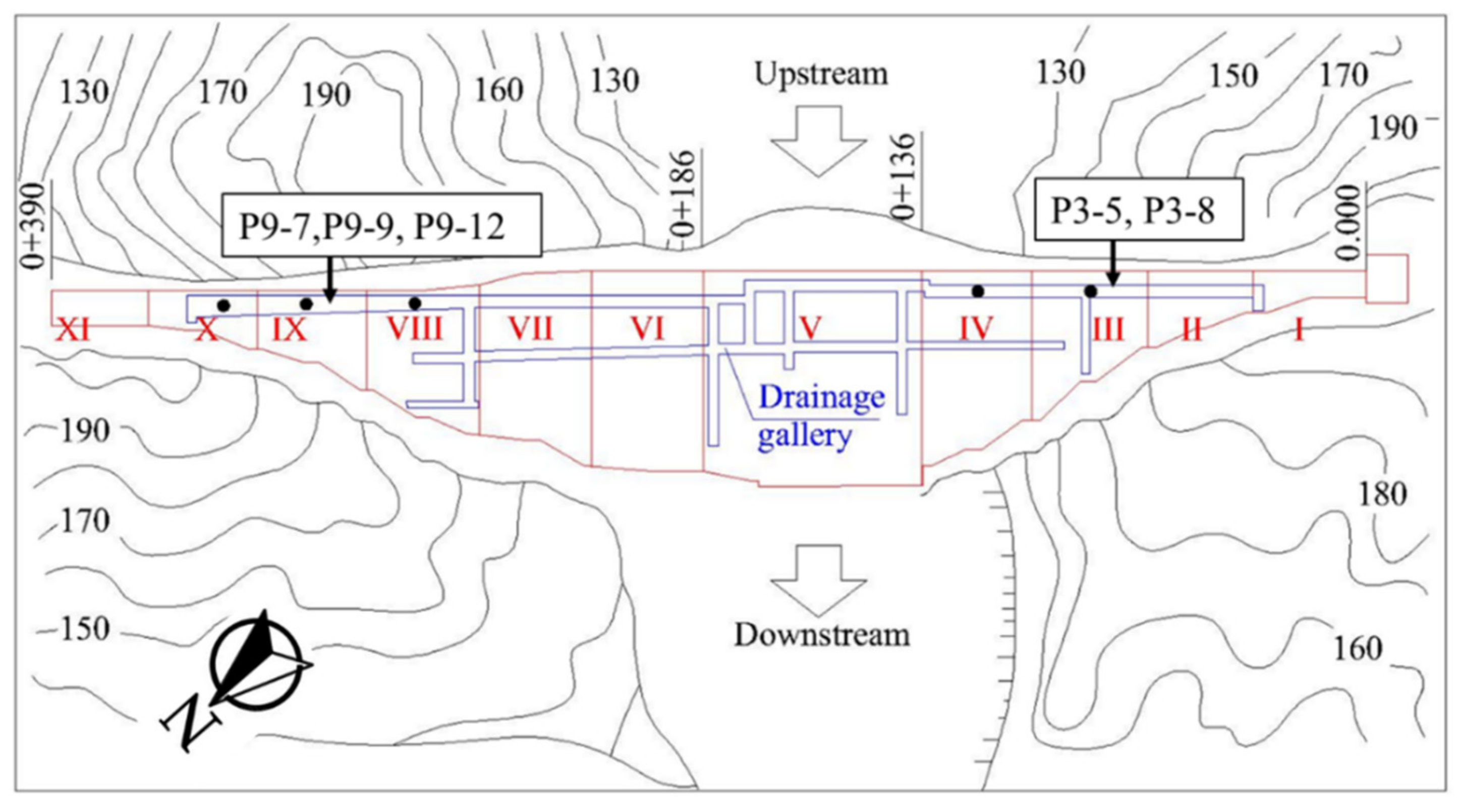
3.1. Dam Engineering and Geological Background

The Wanyao reservoir is located in a U-shaped valley on the Dahe river, about 225 km southwest of Jiangshan City, Zhejiang province, China. Its main functions are water supply, hydroelectric power generation, and preventing floods. The roller compacted concrete dam wall surround the normal concrete core to impound the water. A tunnel and electric equipment are included inside the dam wall. The reservoir harvests surface and groundwater from a 2.12 × ${10}^2$ km² drainage basin. The mean annual rainfall and runoff are about 1.84 × ${10}^3$ mm and 1.10 × ${10}^3$ mm, respectively. The maximum reservoir capacity is approximately 2.23 × ${10}^8$ m³. The reservoir can supply the irrigation water for 2.23 × ${10}^4$ ha farmland, which is significant for the local agriculture. The installed hydro-electric power station behind the dam has a capacity of about 1.26 × ${10}^4$ kW. The mean annual hydro-electricity production is 3.07 × ${10}^7$ kW·h.

The dam is a gravity dam, with 390 m length, constructed with roller compacted concrete and normal concrete. The bottom and top parts of the dam wall are filled with the normal concrete, which is used as the impermeable material on the upstream surface. The roller compacted concrete has the advantages of easy mixing, requiring less construction time, and low-cost materials compared to normal concrete, which is used to construct the core of the dam wall. To reduce the water seepage, an impermeable normal concrete with a thickness of 2 m is placed at the upstream face of the dam wall. The sketch of dam structure is provided on Figure S1. According to the design information, the elevations of observation boreholes range from about 130 to 160 m, and most of them are more than 10 m deep. The water level of the reservoir ranges between 149 and 194 m during different seasons. At the time of conducting the field investigation, the water level was about 190 m. Note that, dam sections I to IX are in contact with an unconfined aquifer while sections X and XI are in contact with an unsaturated zone overlying an unconfined aquifer.

A drainage gallery is constructed inside the dam wall like a tunnel (Figure 3). The boreholes distributed on the gallery are designed to drain away the potential leakage and reduce the uplift pressure. Site geological investigations showed the following [21]: (1) the geological stratum of the dam foundation is mostly pyroclastic rock of Upper Jurassic period; (2) the bedrock is white-gray rigid tuff-lava, which covers alluvial, diluvial, and deluvium, for larger than 100 m thickness; (3) the dam foundation is an aquitard with low permeability; (4) faults in the dam foundation had been grouted during the construction stage. Detailed geological characterization is available in a previous paper [21].

3.2. Field Test Methods

3.2.1. Natural Tracers

To locate the major leakage paths on the dam wall, a field test entailing well-logging using natural tracers (temperature, EC) and the SBDT was conducted in December 2015. Boreholes on dam sections III, IV, VIII, and IX, which showed severe leakage symptoms, were logged in the present study (Figure 3). In total, 48 boreholes with observed leakage were subjected to well-logging using natural tracers. The elevation of most dam sections (III, IV, V, VI, VII, VIII, IX) were below 170 m (Figure 3). Note that, the borehole number represents its location, e.g., P3-9 is the 9th borehole in the dam section III of the dam wall.

An automatic probe provided by Solinst Canada Ltd. was used to record temperature, EC, and water level at every second with a high precision level of 99.5%. Figure 4a is an on-site photo depicting the well-logging procedure. The probe connected to a cable was placed into the bottom of each borehole to log temperature and EC at various depths (Figure 4b).

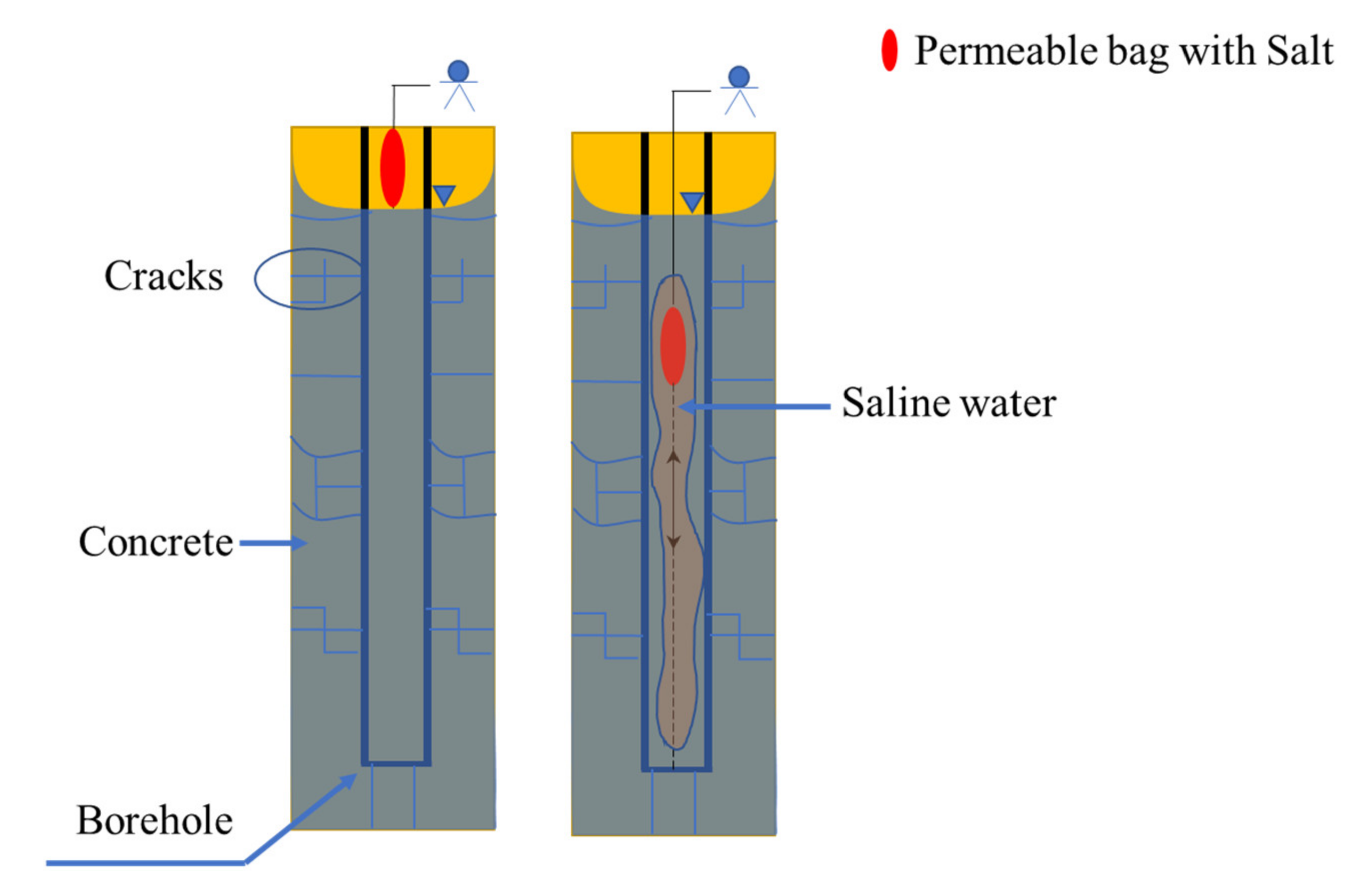
3.2.2. Injection Tracer

In this study, a permeable bag filled with approximately 150 g solid salt was attached to a rope and lowered into the boreholes. A fine-meshed bag (pore size: 1 mm) was filled with a common salt to enable the salt to dissolve quickly into the borehole water. After several up- and downward movements over the whole water column in the borehole, the salt was dissolved and distributed uniformly within the borehole, thereby increasing the EC (Figure 5).

Before the injection, the amount of salt to be applied per borehole needs to be calculated to achieve a concentration higher than the background value. Once the salt is injected, the concentration increases above the original value to the expected concentration. Assuming that the concentration of saline water on borehole is uniform, the lower limit of consumed salt $m_{min}$ (mg) is calculated based on Equation (11):

$$m_{min}=\Delta C·A·L,$$

(11)

where $\Delta C$ is the difference between the original concentration and the expected concentration, and L is the depth of borehole (dm). If the concentration of saline water is non-uniform in the vertical direction, the concentration of salt is a function of the height of the borehole, as shown in the integral form (Equation (12)):

$$m_{min}=A{{\displaystyle \int }}_{x_0}^{x_e}\Delta C\left(x\right)dx.$$

(12)

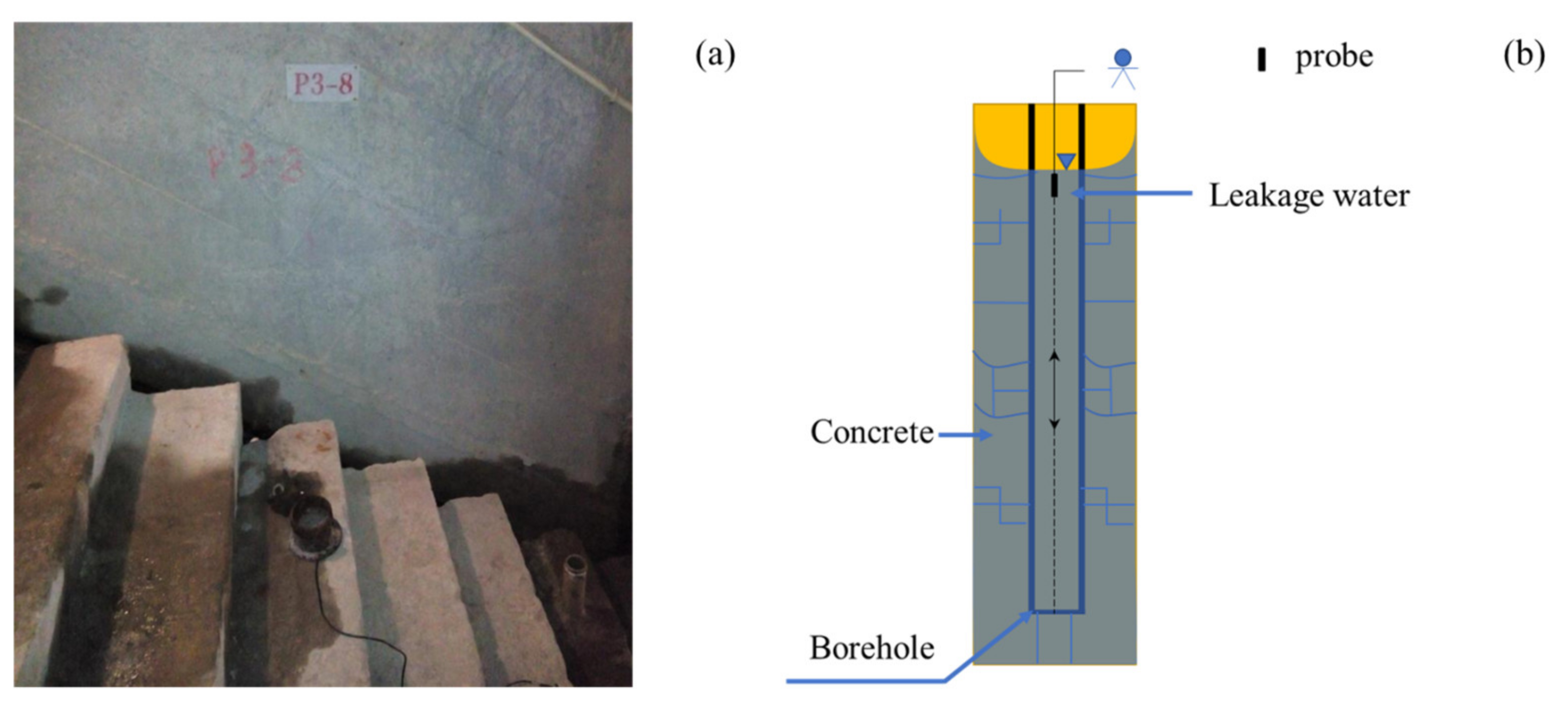
3.2.3. Single Borehole Dilution Tests

In March 2015, with an average ambient air temperature of 14 °C, the SBDT was conducted on sections III and IX of the dam, where the severe leakage existed, based on a previous study [21]. A total of 5 boreholes were used for SBDT: P3-5, P3-8, P9-7, P9-9, and P9-12 and their locations are shown in Figure 3. After injecting common salt for 5 min, the auto-recording probe was slowly lowered into the borehole. When the probe reached the bottom of boreholes, it was slowly pulled out of the water. The recording procedure was repeated to log the EC and the corresponding depth in the boreholes at different times.

4. Results

4.1. Natural Tracer

Temperature and EC profiles of all boreholes inside the dam are given in the Supplementary Material. These are illustrated the following figures: (1) Figure S2 for dam section III, (2) Figure S3 for dam section IV, (3) Figure S4 for dam section VIII and X, and (4) Figure S5 for dam section IX. Comparison of temperature and EC profiles show that temperature profiles have better performance in revealing the flow field in boreholes than EC. The EC of most of the boreholes are even lower than the detection limit of the test equipment.

From temperature logging curves, the highest temperature of the reservoir water was 14 °C (Figure S6), and the water on deeper positions had lower temperature than that in the top positions. This observation means that the temperature of the leakage water with high velocity in the dam wall should be lower than 14 °C. If the leakage source is deeper, the temperature would be closer to 12 °C. Based on previous analysis, temperature profiles shows that the hydraulic behaviors of boreholes can be classified into four clusters: (1) Class 1, characterized by strong connectivity to water reservoir and rapid seepage rate (Figure 6a); (2) Class 2, with strong connectivity to the water reservoir but with a slower seepage rate (Figure 6b); (3) Class 3, having weak connectivity with the shallow part of the reservoir (Figure 6c); and (4) Class 4, with almost no obvious connectivity with the reservoir (Figure 6d).

Table 1. Classification result of boreholes by seepage severity.

Hydraulic Behavior Class	Borehole Numbers
Class 1: High Connectivity on Whole Borehole	P3-6, P4-5, P9-7
Class 2: high connectivity on specific depths	P3-8, P3-12, P3-13, P4-1, P4-2, P9-6, P9-9, P9-10, P9-11, P9-12, P9-13
Class 3: weaken connectivity	P4-3, P4-4, P4-6, P4-7, P4-8, P4-9, P4-10, P4-11, P4-12, P8-2
Class 4: safe boreholes with no obvious connectivity	P3-1, P3-2, P3-3, P3-4, P3-5, P3-9, P3-10, P3-11, P8-1, P8-3, P8-4, P8-5, P8-6, P9-1, P9-2, P9-3, P9-4, P9-5, P9-8, P10-1, P10-2, P10-3, P10-4

. shows the result of the classification of boreholes into the four hydraulic behaviors.

Figure 6 shows the representative profiles of the four classifications of hydraulic behaviors. The categorized borehole temperature profiles are provided in the Supplementary Material (Figures S7–S10). Well-logging data is provided in the Supplementary Material. A summarized description of each class and typical temperature profiles is presented below.

Class 1 has the most obvious seepage behavior (Figure 6a). The shape of the temperature profiles presents a quasi-straight line characteristic. The range of temperature fluctuations with different depths is below 1 °C. For this class, it is difficult to locate the depth of leakage path based on the shape of the temperature profile. In Figure 6a, the curve shows a similar temperature, indicating that the water has little interaction with the surrounding rock. Hence, the water is mainly from fast leakage with high pressure.

Class 2 has a weaker leakage phenomenon than Class 1. Some parts of the temperature profile were higher than 14 °C (the maximum temperature of the reservoir water), but the abrupt or inflection point with obvious fluctuation is evident. The points with low temperature in Class 2 can be used to locate the leakage zone. In Figure 6b, the low temperature zone shows leakage water with high-speed flow into the borehole, and the leakage zone of P3-8 is located at about 250 cm depth. The fast leakage implies that the upper half water in the borehole has limited interaction with the surrounding rocks. However, the rest of the water column in borehole strongly interacts with the surrounding rocks. The leakage zones of Class 2 are summarized in Table S1.

Class 3 has even lower hydraulic connectivity with the reservoir than Classes 1 and 2. Meanwhile, the temperature profile often has a constant slope (Figure 6c). Some parts of the temperature profiles are lower than 14 °C, but the inflection point is not apparent, indicating that no obvious leakage path can be located. In Figure 6c, the part of the curve with a constant slope shows that the water on the boreholes has slow velocity, which means that the water comes from the slow seepage in the dam wall or dam foundation. The strong interaction with the surrounding rock is evident in Figure 6c.

The Class 4 has contrasting hydraulic behaviors relative to the previous three classes. The temperature of Class 4 is higher than 14 °C at every depth, which is the same as that of the upper limit of the reservoir water temperature. This contrasting behavior indicates that boreholes of this class have little connectivity with the reservoir, which means that only limited or no leakage may occur in this class of boreholes (Figure 6d). Water in the boreholes of Class 4 mainly comes from slow seepage, which has a strong interaction with the surrounding rocks.

4.2. Single Borehole Dilution Tests

The well-logging with natural tracers not only showed the flow field of the boreholes, but also provided the background values of temperature and EC. Most of the boreholes have low EC values, which are suitable to conduct SBDT. Note that, in Figure 7, Figure 8 and Figure 9, $t_0$ represents the initial time for the background curve, and $t_1$, $t_2$, $t_3$, $t_4$, $t_5$, represent the subsequent time-steps for the observed curves after injecting tracer at different times in a sequence. The time intervals of every logging are shown in Table S2.

Figure 7 shows little variations of EC in the P3-5 and P3-8 curves at different times, but these have different meanings. After injecting the tracer, the breakthrough curves of the boreholes get obviously larger, which indicates that the salt injection and mixing was successful. For P3-5, the slight variation reveals a little change in EC, which means that the leakage brings little tracer-laden water out. In other words, the leakage in P3-5 is weak. For P3-8, the little variation is similar to that in P3-5, but it has a low EC zone at the top. The result from the permeable bag was always pulled out of the borehole, as it is difficult to form a low EC zone on a shallow part. A possible reason was that the tracer-free water quickly replaced the tracer-laden water, thus the little short-lived changes were missed during the observations. The movement of vertical flow on a shallow part of P3-8 should be higher than the length of the low EC zone between the injection time and the first observation. As mentioned in the methods section, the first observation was made 5 min after the injection. Hence, the vertical mean velocity of the shallow zone of P3-8 should be higher than 1.66 cm/s, which is calculated by the distance of the borehole ratio observation time interval. This situation is an extreme scenario of Equation (6), because the upper limit is unknown.

EC profiles of dam section IX (P9-7, P9-9, P9-12) show more obvious changes in EC, especially P9-7. The curve of EC for borehole P9-7 decreases to values below the detection limit at the second observation time $t_2$, which means that the whole water column is replaced by fresh water. Similar to P3-8, the movement of vertical flow of P9-7 is longer than the length of the borehole between the first and second observations times. In other words, the vertical mean velocity of P9-7 is higher than 0.95 cm/s. The calculation is similar to P3-8, which is the extreme scenario of Equation (6). The EC profiles of boreholes P9-9 and P9-12 appear obvious, with differences that would be beneficial to analyze further. The EC curve of P9-9 is a typical case of upper vertical flow. For P9-12, the EC curve is a typical shape with high flow velocity, which can be found in a tracer-related study [20]. Figure 8 and Figure 9 show the breakthrough curves of P9-9 and P9-10 at different times. In these two boreholes, the time interval and EC curves are used to calculate the distance ranges of flow by Equation (6). Based on Equation (6), the mean velocity value of P9-9 and P9-12 are derived (

Table 2. The effective vertical velocity of P9-9 and P9-12 calculated using Equation (6).

Boreholes	Test	Lower Limit of Velocity: cm/s	Upper Limit of Velocity: cm/s	Mean Velocity: cm/s	Stand Deviation:	Overall Mean of Tests: cm/s
P9-9 (Class 2)	1	0.20	0.28	0.24	0.04	0.255
	2	0.26	0.28	0.27	0.01
	3	0.21	0.22	0.215	0.005
	4	0.27	0.32	0.295	0.025
P9-12 (Class 2)	1	0.17	0.71	0.44	0.27	0.505
	2	0.27	0.82	0.545	0.275
	3	0.38	0.71	0.545	0.165
	4	0.37	0.61	0.49	0.12

). A detailed limit of distance for each test is provided in Table S3.

For Figure 9, three fluctuation points are evidently found in the curve at the first observation time $t_1$ but only two of them still exist in the next observation. Therefore, two locations around 450 and 600 cm depth are speculated to have a more severe leakage zone than the location around 1200 cm depth.

4.3. Validation

The validation results are based on the comparison of results from the natural tracer test and SBDT. Meanwhile, the site investigation of leakage and historical observation data are also used. Figure 10 shows the temperature profiles of boreholes used to conduct SBDT. According to the four hydraulic clusters identified based on the natural tracer test in the previous section, the five boreholes are classified into: (1) Class 1 with high connectivity on whole borehole (P9-7); (2) Class 2 with high connectivity at some parts of borehole (P3-8, P9-9, P9-12); (3) Class 4: safe boreholes with no evident connectivity (P3-5).

In summary, the SBDT shows similar results to those of the natural tracer test. Specifically, P3-5 has a weak connectivity with the reservoir, which is consistent with the results for the temperature profiles (Figure 10). P9-7 has a high vertical velocity, which is similar to the results from natural tracers. P3-8 and P9-9 are located in the leakage zone with clear infection points, which are similar to the results from the natural tracer test (Table S1). In borehole P9-12, one leakage point, which is located at 600 cm, was found in both the temperature profile (Figure 10) and SBDT (Figure 9), while another weaker leakage point located at 450 cm was only detected by the SBDT (Figure 9). A comparison of the natural tracer test to SBDT shows that the latter has a more powerful ability to detect potential leakage zones than the former. In addition, unlike the natural tracer test, SBDT provided the range of vertical flow velocities in P9-9 and P9-12.

Results of on-site investigation showed that P9-7 had obvious leakage phenomenon with gushing water. In addition, the historical observation shows that sections VII and IX of the dam wall had large leakage. These field observations further corroborate the results of the SBDT method. However, field data on leakage rates were not available for the other individual boreholes where the seepage rates were estimated using the SBDT method.

5. Discussion

The detection and estimation of seepage is critical in the operation and maintenance of hydraulic structures such as dams, but existing techniques have a number of limitations. The low-cost, environmental friendliness, and relative simplicity of natural and artificial tracer tests render them attractive for detecting and quantifying seepage in hydraulic structures. Yet, until now, tracer tests have been limited to the detection of seepage flow paths in groundwater systems, but their application to understanding seepage problems in dams has received limited attention. Moreover, a single tracer test and corresponding algorithm that enable the determination of both seepage flow paths and seepage rates have been lacking. Therefore, the present field-based study addressed these limitations by developing and applied a new tracer technique for quantifying seepage—the single borehole dilution test (SBDT). The present study makes three key contributions to the current knowledge on seepage problems. Firstly, a novel algorithm was developed and then applied to analyze the SBDT data. Secondly, using the case study of a dam, the application of the SBDT to determine seepage under field conditions is demonstrated. Finally, a qualitative validation of the SBDT results against other field data, including observed seepage, is conducted.

The SBDT, including the novel algorithm was demonstrated to have the unique capacity to serve a dual function: (1) detection of seepage flow paths, and (2) quantifying seepage flow velocities. In addition, the SDBT had better capacity to detect leakage zones which were not evident in analysis based on conventional tracer tests. This indicates a key novelty compared to earlier studies based on conventional tracer tests and analysis [10,20,28]. While conventional tracer tests require both uniform and point injection data to estimate seepage rates, the SBDT estimates the range of seepage flow velocities based only on uniform injection data. For example, compared to earlier studies using tracer tests on dam leakage detection [10,25], the SBDT has the ability to calculate the range of mean seepage velocity. Thus, due to its dual function, the SBDT requires putatively lower data, equipment, and costs than conventional tracer-based tests based on both uniform and point injection data.

Note that, in the present study, the SBDT was limited to dam leakage detection, because of the ease of measurement and the homogeneity of the concrete material. However, besides dams, a few studies also exist on the application of SBDT for characterization or quantification on aquifer [27,28,29,31]. This points to the possibility to extend and adapt the SBDT to other seepage problems in hydraulic structures. As demonstrated in the present paper, the SBDT and its algorithm are a tractable technique. This is because, without a complex derivation, the foundational theory of this SBDT and the analytical algorithm can be understood easily. The necessary equipment only includes an auto-recording probe, a permeable bag, ropes/cables, and soluble salt. In the future, the development on professional equipment would improve this method. Thus, the SBDT provides both researchers and practitioners another potential tool for the determination of seepage in hydraulic structures.

In the present study, validation was limited to a qualitative comparison of the SBDT results to that of natural tracers and historical seepage data. However, a quantitative validation entailing the use of statistical tests was not feasible due to a number of potential difficulties. In the case of dam leakage investigated in the present study, these difficulties include: (1) unlike aquifers, additional boreholes cannot be installed in the pre-existing concrete dam to validate the results; and (2) the tracer test in the boreholes in the dam wall includes the solute transport in the subsurface water and surface water, which makes it difficult to develop a numerical experiment consistent with the reality. To our knowledge, there is no available code to simulate such a complex solute mixing and flow scenario.

Further research is necessary to validate the new approach on other hydraulic structures with the seepage phenomenon. Moreover, a comparison of the results of the new SBDT method to conventional seepage analysis methods is required. In the future, we intend to conduct further studies of this problem in the laboratory with a synthetic model or prototype of a dam with the leakage phenomenon, coupled with 2-D and 3-D numerical simulations. In such future studies, several seepage scenarios can be investigated, including: (1) varying the location or depth of the leakage zone in the dam wall, (2) altering the water level in the dam, and (3) simulating changes in material hydraulic properties due to aging and weathering. Moreover, future 3-D modelling may also investigate the leakage, structural stability, and safety of the whole dam rather than specific dam sections, as investigated in the present study.

6. Conclusions

The present study investigated the leakage problem on the Wanyao dam based on tracer tests. The spatial distribution of temperature and EC on 48 boreholes are obtained based on well-logging technique with natural tracers. A new way of calculating range of mean vertical velocity on open borehole is proposed, which is based on the Law of Mass. The proposed approach compares the residual tracers to obtain the losing mass, and solving the integral Equation of EC to get the range of the mean vertical velocity.

Using well-logging of natural tracers, boreholes are categorized into four classes based on hydraulic behavior. Classes 1 and 2 had strong connectivity and a severe leakage problem compared to Classes 3 and 4, which had limited to negligible seepage. The application of the SBDT to five boreholes revealed the following: (1) P3-5 is confirmed to have weak evidence of leakage; (2) The vertical velocity of P3-8 and P9-7 is more than 1.66 cm/s and 0.95 cm/s, respectively; (3) In boreholes P9-9 and P9-12, the mean velocities of the tests are 0.26 and 0.51 cm/s, respectively; and (4) For P9-12, an extra leakage path is located at a depth of 450 cm, which is easy to miss in the curves of the natural tracers. Taken together, these findings provide further insights into the seepage problem, which are not evident when using the conventional tracer method, as described in Huang et al. [21].

Finally, we conclude that:

(1)

The natural tracer test is an effective method for detecting the leakage of hydraulic engineering structures such as dams. In this study, the leakage path of a borehole is located by the temperature profiles. The EC of boreholes is too low to analyze, but it also provides background value for SBDT. Hence, it is recommended that the tracer test coupled well-logging technique can detect or investigate leakage problems;

(2)

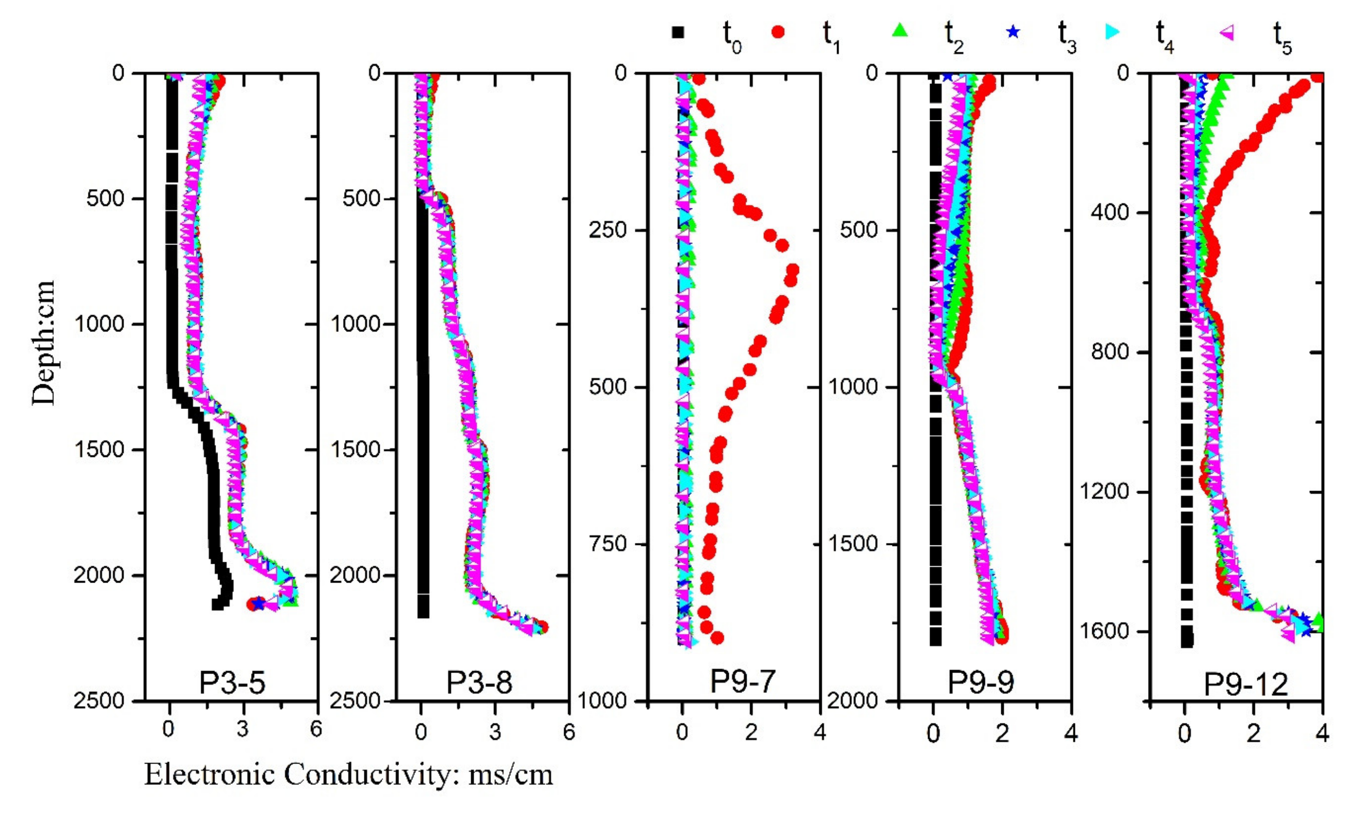
Based on background value, SBDT has good performance on locating and quantifying leakage than conventional tracer methods. Specifically, SBDT locates an extra leakage path in P9-12, which is not apparent in the natural temperature profile. The results of SBDT were also validated by the natural tracer test, and field observations;

(3)

The proposed SBDT method is successful in calculating the range of mean vertical velocity in open boreholes, which demonstrates its feasibility. Based on the proposed method, the quantitative comparison of leakage severity between two boreholes is possible;

(4)

Although the present study provides interesting findings, the proposed SBDT method still requires further improvement. To this end, future directions, including quantitative validation, and 2-D and 3-D modelling were highlighted. In addition, there is a need to adapt the method to enable it to estimate the specific range of vertical velocities, and whether or not such velocities are consistent with field observations.

References

1. Lehner, B.; Liermann, C.R.; Revenga, C.; Vörömsmarty, C.; Fekete, B.; Crouzet, P.; Döll, P.; Endejan, M.; Frenken, K.; Magome, J.; et al. High-Resolution Mapping of the World’s Reservoirs and Dams for Sustainable River-Flow Management. Front. Ecol. Environ. 2011, 9, 494–502. [Google Scholar] [CrossRef]
2. Ikard, S.J.; Revil, A.; Schmutz, M.; Karaoulis, M.; Jardani, A.; Mooney, M. Characterization of Focused Seepage Through an Earthfill Dam Using Geoelectrical Methods. Groundwater 2014, 52, 952–965. [Google Scholar] [CrossRef] [PubMed]
3. Minsley, B.J.; Burton, B.L.; Ikard, S.; Powers, M.H. Hydrogeophysical Investigations at Hidden Dam, Raymond, California. J. Environ. Eng. Geophys. 2011, 16, 145–164. [Google Scholar] [CrossRef]
4. Demanet, D.; Jongmans, D. Seismic Tomography Survey under the La Gileppe Dam. Geol. Soc. Eng. Geol. Spec. Publ. 1997, 12, 175–182. [Google Scholar] [CrossRef]
5. Di Prinzio, M.; Bittelli, M.; Castellarin, A.; Pisa, P.R. Application of GPR to the Monitoring of River Embankments. J. Appl. Geophys. 2010, 71, 53–61. [Google Scholar] [CrossRef]
6. Xu, X.; Zeng, Q.; Li, D.; Wu, J.; Wu, X.; Shen, J. GPR Detection of Several Common Subsurface Voids inside Dikes and Dams. Eng. Geol. 2010, 111, 31–42. [Google Scholar] [CrossRef]
7. Al-Fares, W. Contribution of the Geophysical Methods in Characterizing the Water Leakage in Afamia B Dam, Syria. J. Appl. Geophys. 2011, 75, 464–471. [Google Scholar] [CrossRef]
8. Bièvre, G.; Lacroix, P.; Oxarango, L.; Goutaland, D.; Monnot, G.; Fargier, Y. Integration of Geotechnical and Geophysical Techniques for the Characterization of a Small Earth-Filled Canal Dyke and the Localization of Water Leakage. J. Appl. Geophys. 2017, 139, 1–15. [Google Scholar] [CrossRef]
9. Bair, E.S.; Parizek, R.R. Detection of Permeability Variations by a Shallow Geothermal Technique. Groundwater 1978, 16, 254–263. [Google Scholar] [CrossRef]
10. Wang, T.; Chen, J.; Li, P.; Yin, Y.; Shen, C. Natural Tracing for Concentrated Leakage Detection in a Rockfill Dam. Eng. Geol. 2019, 249, 1–12. [Google Scholar] [CrossRef]
11. Gubareva, T.S.; Boldeskul, A.G.; Gartsman, B.I.; Shamov, V. V Analysis of Natural Tracers and Genetic Runoff Components in Mixing Models: Case Study of Small Basins in Primor’e. Water Resour. 2016, 43, 629–639. [Google Scholar] [CrossRef]
12. Hilberg, S. Review: Natural Tracers in Fractured Hard-Rock Aquifers in the Austrian Part of the Eastern Alps—Previous Approaches and Future Perspectives for Hydrogeology in Mountain Regions. Hydrogeol. J. 2016, 24, 1091–1105. [Google Scholar] [CrossRef]
13. Mudarra, M.; Andreo, B.; Marín, A.I.; Vadillo, I.; Barberá, J.A. Combined Use of Natural and Artificial Tracers to Determine the Hydrogeological Functioning of a Karst Aquifer: The Villanueva Del Rosario System (Andalusia, Southern Spain). Hydrogeol. J. 2014, 22, 1027–1039. [Google Scholar] [CrossRef]
14. Robert, T.; Caterina, D.; Deceuster, J.; Kaufmann, O.; Nguyen, F. A Salt Tracer Test Monitored with Surface ERT to Detect Preferential Flow and Transport Paths in Fractured/Karstified Limestones. Geophysics 2012, 77, B55–B67. [Google Scholar] [CrossRef]
15. Ravbar, N.; Barberá, J.A.; Petrič, M.; Kogovšek, J.; Andreo, B. The Study of Hydrodynamic Behaviour of a Complex Karst System under Low-Flow Conditions Using Natural and Artificial Tracers (the Catchment of the Unica River, SW Slovenia). Environ. Earth Sci. 2012, 65, 2259–2272. [Google Scholar] [CrossRef]
16. Yilmaz, S.; Koksoy, M. Electrical Resistivity Imaging and Dye Tracer Test for the Estimation of Water Leakage Paths from Reservoir of Akdeğirmen Dam in Afyonkarahisar, Turkey. Environ. Earth Sci. 2017, 76, 829. [Google Scholar] [CrossRef]
17. Poulsen, D.L.; Cook, P.G.; Simmons, C.T.; McCallum, J.M.; Noorduijn, S.L.; Dogramaci, S. A Constant Rate Salt Tracer Injection Method to Quantify Pumped Flows in Long-Screened or Open Borehole Wells. J. Hydrol. 2019, 574, 408–420. [Google Scholar] [CrossRef]
18. Binet, S.; Joodi, A.; Joigneaux, E.; Albéric, P.; Gutierrez, A. Localisation of a Reactive Transport Zone in a Saturated Karstic Conduit Deduced from Natural and Artificial Tracer Tests. In Advances in Research in Karst Media; Andreo, B., Carrasco, F., Durán, J.J., LaMoreaux, J.W., Eds.; Springer: Berlin/Heidelberg, Germany, 2010; pp. 123–129. ISBN 978-3-642-12486-0. [Google Scholar]
19. Lee, J.-Y.; Kim, H.-S.; Choi, Y.-K.; Kim, J.-W.; Cheon, J.-Y.; Yi, M.-J. Sequential Tracer Tests for Determining Water Seepage Paths in a Large. Eng. Geol. 2007, 89, 300–315. [Google Scholar] [CrossRef]
20. Maurice, L.; Barker, J.A.; Atkinson, T.C.; Williams, A.T.; Smart, P.L. A Tracer Methodology for Identifying Ambient Flows in Boreholes. Ground Water 2011, 49, 227–238. [Google Scholar] [CrossRef]
21. Huang, Y.; Hou, X.; Fu, Z.; Wang, J. Detection of Leakage Paths at the Wanyao Dam Body in Southwest China by Hydrochemical Analysis and Tracer Testing. Environ. Earth Sci. 2018, 77, 791. [Google Scholar] [CrossRef]
22. Medici, G.; West, L.J. Groundwater Flow Velocities in Karst Aquifers; Importance of Spatial Observation Scale and Hydraulic Testing for Contaminant Transport Prediction. Environ. Sci. Pollut. Res. 2021, 28, 43050–43063. [Google Scholar] [CrossRef] [PubMed]
23. Pitrak, M.; Mares, S.; Kobr, M. A Simple Borehole Dilution Technique in Measuring Horizontal Ground Water Flow. Groundwater 2007, 45, 89–92. [Google Scholar] [CrossRef] [PubMed]
24. Maurice, L.D.; Atkinson, T.C.; Barker, J.A.; Williams, A.T.; Gallagher, A.J. The Nature and Distribution of Flowing Features in a Weakly Karstified Porous Limestone Aquifer. J. Hydrol. 2012, 438–439, 3–15. [Google Scholar] [CrossRef]
25. Dong, H.; Chen, J.; Li, X. Delineation of Leakage Pathways in an Earth and Rockfill Dam Using Multi-Tracer Tests. Eng. Geol. 2016, 212, 136–145. [Google Scholar] [CrossRef]
26. Jamin, P.; Goderniaux, P.; Bour, O.; Le Borgne, T.; Englert, A.; Longuevergne, L.; Brouyère, S. Contribution of the Finite Volume Point Dilution Method for Measurement of Groundwater Fl Uxes in a Fractured Aquifer. J. Contam. Hydrol. 2015, 182, 244–255. [Google Scholar] [CrossRef]
27. Maldaner, C.H.; Munn, J.D.; Coleman, T.I.; Molson, J.W.; Parker, B.L. Groundwater Flow Quantification in Fractured Rock Boreholes Using Active Distributed Temperature Sensing Under Natural Gradient Conditions. Water Resour. Res. 2019, 55, 3285–3306. [Google Scholar] [CrossRef]
28. Agbotui, P.Y.; West, L.J.; Bottrell, S.H. Characterisation of Fractured Carbonate Aquifers Using Ambient Borehole Dilution Tests. J. Hydrol. 2020, 589, 125191. [Google Scholar] [CrossRef]
29. Fahrmeier, N.; Goeppert, N.; Goldscheider, N. Comparative Application and Optimization of Different Single-Borehole Dilution Test Techniques. Hydrogeol. J. 2020, 29, 199–211. [Google Scholar] [CrossRef]
30. Maldaner, C.H.; Quinn, P.M.; Cherry, J.A.; Parker, B.L. Improving Estimates of Groundwater Velocity in a Fractured Rock Borehole Using Hydraulic and Tracer Dilution Methods. J. Contam. Hydrol. 2018, 214, 75–86. [Google Scholar] [CrossRef]
31. Gomo, M. Effects of Artefacts on Natural Gradient Single-Borehole Tracer Dilution Tests. Nat. Resour. Res. 2020, 29, 2227–2235. [Google Scholar] [CrossRef]
32. Lewis, A.S.; Lucchetti, R.E. Nonsmooth Duality, Sandwich, and Squeeze Theorems. SIAM J. Control Optim. 2000, 38, 613–626. [Google Scholar] [CrossRef]
33. Balk, M.; Bose, M.; Ertem, G.; Rogoff, D.A.; Rothschild, L.J.; Freund, F.T. Oxidation of Water to Hydrogen Peroxide at the Rock–Water Interface Due to Stress-Activated Electric Currents in Rocks. Earth Planet. Sci. Lett. 2009, 283, 87–92. [Google Scholar] [CrossRef]
34. Walter, D.; Dietmar, K.; Arnd, K.; Heribert, M.; Ferdinand, N.; Werner, R. Point Dilution Methods of Investigating Ground Water Flow by Means of Radioisotopes. Water Resour. Res. 1968, 4, 125–146. [Google Scholar]
35. Brouyère, S.; Batlle-aguilar, J.; Goderniaux, P.; Dassargues, A. A New Tracer Technique for Monitoring Groundwater Fluxes: The Finite Volume Point Dilution Method. J. Contam. Hydrol. 2008, 95, 121–140. [Google Scholar] [CrossRef] [PubMed]
36. Kolesnikova, L.N. Guidebook on Nuclear Techniques in Hydrology. At. Energ. 1984, 57, 413–414. [Google Scholar]
37. Lewis, E. The Practical Salinity Scale 1978 and Its Antecedents. IEEE J. Ocean. Eng. 1980, 5, 3–8. [Google Scholar] [CrossRef]
38. Widodo, C.S.; Sela, H.; Santosa, D.R. The Effect of NaCl Concentration on the Ionic NaCl Solutions Electrical Impedance Value Using Electrochemical Impedance Spectroscopy Methods. AIP Conf. Proc. 2018, 2021, 050003. [Google Scholar] [CrossRef]
39. Lide, D.R. CRC Handbook of Chemistry and Physics; CRC Press: Boca Raton, FL, USA, 2004; Volume 85. [Google Scholar]
Figure 1. Theoretical concentration profiles of uniform injection at: (a) initial time t 0 ; (b) first observation time t 1 ; (c) second observation time t 2 ; (d) at third observation time t 3 . (e) the overlay chart of (bd). Note that the time interval between two observation times is equal.
Water 14 01448 g001
Figure 2. Illustration of the integral of concentration curve versus depth at: (a) first observation time t 1 ; (b) second observation time t 2 ; (c) third observation time t 3 ; (d) is the overlap of previous curves.
Water 14 01448 g002
Figure 3. Top view of the dam. The black circles represent the boreholes where tracer tests were conducted. Locations of boreholes where SBDT was conducted are shown by two black circles which represent P9-7, P9-9, P9-12, and P3-5, P3-8, respectively.
Water 14 01448 g003
Figure 4. Illustration of well-logging with natural tracer: (a) on-site photo; (b) sketch of the logging process.
Water 14 01448 g004
Figure 5. Illustration of injections with permeable bag containing salt.
Water 14 01448 g005
Figure 6. Representative temperature profiles of Classes 1, 2, 3, and 4 of the boreholes based on hydraulic behaviors. (ad) represent the typical curves of Classes 1, 2, 3, and 4, respectively.
Water 14 01448 g006
Figure 7. Overlapped EC profiles of boreholes P3-5, P3-8, P9-7, P9-9, and P9-12 at different times.
Water 14 01448 g007
Figure 8. EC profiles of P9-9 at different times.
Water 14 01448 g008
Figure 9. EC profiles of P9-12 at different times.
Water 14 01448 g009
Figure 10. Temperature profiles of boreholes from the natural tracer test.
Water 14 01448 g010