Article

Analysis of Climate Variability in a Time Series of Precipitation and Temperature Data: A Case Study in Cartagena de Indias, Colombia

by
Alfonso Arrieta-Pastrana
,
Manuel Saba
* and
Adriana Puello Alcázar
Civil Engineering Program Faculty of Engineering, University of Cartagena, Cartagena de Indias 130001, Colombia
*
Author to whom correspondence should be addressed.
Water 2022, 14(9), 1378; https://doi.org/10.3390/w14091378
Submission received: 15 March 2022 / Revised: 22 April 2022 / Accepted: 22 April 2022 / Published: 24 April 2022

Abstract

:
Anthropogenic climate change is a global trend, hitherto incontrovertible, causing immense social and economic damage. Although the this is evident at the global level, at the local level, there is still debate about the most appropriate analyses to support this fact. This debate is particularly relevant in developing countries, such as Colombia, where there is a significant lack of data at the local level that require analysis and interpretation. Consequently, studies are often superficially conducted to support climate change theory at the local level. However, such studies are then used to design hydraulic infrastructure, with potential catastrophic errors for human and environmental health. In this study, we sought evidence of climate change through an analysis of a series of data on temperature (maximum, mean and minimum), as well as total annual and maximum rainfall in 24 h registered at the Rafael Nuñez Airport station in the city of Cartagena, Colombia, from 1941 to 2015. The hypotheses of homogeneity, trend, stationarity and non-stationarity were analyzed. Problems of non-homogeneity and the presence of periodicity in the analyzed series were found, showing a trend and apparent non-stationarity in the original series. This could be associated with the effects of climate change. In this case, no correlation was found between temperatures and rainfall. Spectral analysis was performed for all series, and residual series were generated by extracting the harmonics of greatest significance. It was found that the series data generated from the third harmonic are generally stationary and without trend. Therefore, the trend and non-stationarity of the original series are due to problems of non-homogeneity and periodicity in the series. In the results of the stationarity test conducted according to the Phillips–Perron criterion, all series were non-stationary. For the two additional criteria of stationarity tests, 40% were shown to be stationary, and 60% were non-stationary. Specifically, non-homogeneity problems and apparent trends associated with climate change could have negative implications for the design of drainage systems.

1. Introduction

The effects of climate change have been mainly associated with the gradual change in long-term average temperature. This hypothesis, which has been internationally proposed and discussed [1], impacts the magnitude of average and extreme rainfall, as well as the maximum intensities that are used in the design of engineering works. It has been argued that climate change has increased the change in the natural limits of the environment, creating more frequent extreme climate events.
Furthermore, it has been claimed that the effect of climate change on hydrological series ruins the stationarity hypothesis, which has been questioned in recent years by some authors, who stated that it has died and that it is impossible to revive it because anthropogenic effects on the climate are increasing [2]. The concern is so great that in 2010, an interinstitutional workshop involving entities that manage water in the United States was proposed to discuss the issue of stationarity [3]. Some think that it was a premature death [4], but other authors believe that stationarity is immortal, stating that the change criterion has been confused with “non-stationarity” and that all hydrological models are affected by uncertainty and must include a random component that is stationary [5]. The concept that stationarity is dead was reaffirmed and clarified by several authors [6]; it was argued that the term “non-stationarity” has been misused as a synonym for change and that the stochastic dependence of the models has been interpreted as non-stationarity [7].
Germán Poveda and Álvarez (2012) [8] stated that “climate change, climate variability and deforestation contribute to the collapse of the stationarity hypothesis”, generating important implications for hydrological design. As an emergent criterion of analysis, Obeysekera and Salas (2014) [9] proposed the criterion of non-stationarity and non-homogeneous distribution. The concept of the frequency of extreme events is created when the extreme values are non-stationary [8,9,10]. Examples of these theories have been applied in sectors of the city of Cartagena [11], considering non-stationary series.
In some regions [12], the local average temperature has been related to the extreme daily values of precipitation, revealing that extreme rainfall events are related, with a high probability, to temperatures of 30 °C. In most South Asian countries, general changes in precipitation and temperature have produced alterations in water availability. As a general phenomenon, it has been argued that in most countries in South Asia, the intensity of rainfall has increased [13].
The rainfall patterns used for the design of drainage works [14] have been proposed without considering climate change. However, it has been shown that rainfall can be affected by temperature and that the maximum flow used for designs can also be affected. In this study, we found that if an area is warmer, the rain pattern is less uniform, leading to more intense peaks. In a study carried out in India [15], the authors suggested that temporal trends in temperature affect the frequency and magnitude of the intensity of rain, modifying the uniformity of rainfall.
According to a report of the Economic Commission for Latin America and the Caribbean (CEPAL, abbreviated from the Spanish name) [16], gradual changes now occur that make it difficult to separate climate change from the climate variability experienced in the past.
In the case of Colombia, several authors have searched for evidence of climate change in the hydrological and climatic records [17], finding warming trends in the minimum and average temperatures; however, the precipitation series did not show evidence of climate change.
In response to the effect that climate change may have on hydrological design parameters, the Ministry of Housing, City and Territory of the Republic of Colombia, in Article 135 of Resolution 0330 of 8 June 2017, highlighted the need to consider the intensity, the effects of variability and climate change in Colombia in the calculations used for the design of engineering works.
In the present study, we proposed to search for evidence of effects associated with climate change in the records of the precipitation time series that could produce alterations in the hydrological design parameters of engineering works at the local level. It should be considered that Cartagena’s monitoring station suffered several changes in its location instrumentation in the past. The data considered are time series of maximum rainfall in 24 h, total annual rainfall, annual minimum temperature, annual average temperature and annual maximum temperature from 1941 to 2015 taken at the Rafael Núñez Airport station in the city of Cartagena, Colombia, provided by the Institute of Hydrology, Meteorology and Environmental Studies (IDEAM, abbreviated from its name in Spanish).

2. Location of the Study Area

The study zone chosen was the city of Cartagena, located in the central region of the Colombian Caribbean, at approximately 10°25′20″ N, 75°32′25″ W. Cartagena is a tourist city and has been declared a Historical and Cultural Heritage of Humanity by UNESCO (Figure 1).
According to the climatological atlas of Colombia from the Colombian Institute of Hydrology, Meteorology and Environmental Studies (IDEAM, for its initials in Spanish), precipitation registers low volumes that do not exceed 1000 mm per year. The intra-annual regime is approximately bimodal, with a main rainy season in September, October and November and two dry seasons from December to April and in June–July. The average number of rainy days during the year is 50 to 100. Due to its physiognomy, without major mountainous accidents, the temperature distribution is very homogeneous, registering a little more than 28 °C. According to the Caldas–Lang indices for climatic classification, the climate presented is warm, semi-arid and semi-humid.

3. Methodology

For the study, the time series of the IDEAM station with the code name 14015020, located at the Rafael Núñez Airport in the city of Cartagena, Colombia, were selected. The series of total annual rainfall, maximum rainfall in 24 h, minimum annual temperature, mean annual temperature and maximum annual temperature were selected for the period between 1941 and 2015. For statistical analysis of the series, XLSTAT® software was used.
The data were reviewed. There were some missing data, such as the maximum temperature and minimum temperature for the years 1941, 1942 and 1960, as well as the minimum temperature for the years 1951 and 1952. The missing data were filled using the principle of conservation of the mean and variance to calculate the descriptive statistics of all series. The initial trend of the series was analyzed with the original data, filling in the missing data. A homogeneity test was performed on all series, considering the criteria of Pettitt [18,19], SNHT [20,21], Buishand [22] and Von Neuman [23]. Additionally, three stationarity tests were carried out: the Dickey–Fuller test [24], the Phillips–Perron test [25] and the KPSS test [26,27]. The series were corrected for non-homogeneity. The Mann–Kendall test was applied to analyze the trend [19,28,29]. A spectral analysis was performed on the series after correction for homogeneity to determine the significant periodicities of the series.
In addition, the eight harmonic components that showed the greatest significance in each of the series were selected. Residual series of analysis were generated by extracting the periodic functions with the two most significant frequencies from the original series, with three, four and eight significant frequencies. Finally, the stationarity and trend tests used in the original series were applied to the series adjusted for non-homogeneity and to the generated residual functions. In the literature, the Mann–Kendall test has been used to execute analyses of hydroclimatic trends and to detect seasonal and annual droughts in a basin, revealing significant warming throughout the basin [30]. On the other hand, the Mann–Kendall test has been used to detect the trend and change point in hydroclimatic variables during a specific period in a basin, demonstrating good performance [31].

4. Results

The data series taken from IDEAM are shown in Appendix A, with the original data presented in the series on the left. The values shaded in blue represent doubtful values, whereas those in gray are the missing data. The series in green were filled with random data that met the mean and variance.
In Table 1, the descriptive statistical parameters of the original series provided by IDEAM are presented. It can be seen that the coefficients of variation of the maximum rainfall in 24 h (P24) and the total annual rainfall (PT) are similar (0.40 and 0.46), and the temperatures (mean, maximum and minimum) are lower (0.02, 0.05 and 0.06). The temporal correlation coefficient shows an intermediate value for P24 and PT (0.39 and 0.45), a significant value for the minimum temperature (Tmin) (0.66) and a very low correlation with the mean and maximum temperature.
In Figure 2, the IDEAM data are presented for the maximum precipitation in 24 h (P24) and the total annual precipitation (PT), plotted as a function of time, to which a linear function was fitted in order to visualize the trend. The results show low correlation coefficients and an increase in the mean values of 0.68 mm per year for maximum precipitation in 24 h (P24), as well as an increase of 8.85 mm per year for total annual precipitation (PT).
Figure 3 presents the maximum, mean and minimum temperatures, in degrees Celsius, recorded at the Rafael Núñez Airport station. To visualize the possible trends, a linear function is presented. The series of maximum rainfall shows a very slight decreasing trend of 0.0068 degrees per year. The series of mean temperatures tends to be constant, with a slight decrease of 0.00004 degrees per year and very low correlations. The minimum temperature shows a significant increase of 0.0357 °C per year and a significant coefficient of determination (R2 = 0.4327).

4.1. Homogeneity Tests

To evaluate the consistency of the historical data, XLSTAT software was used, and the Pettitt, SNHT, Buishand and Von Neuman homogeneity tests were performed on the P24, PT, Tmax, Tmean and Tmin series. In all cases, the results of the Pettitt, SNHT and Buishand tests showed that the data are not homogeneous, with days on which there were changes in the data. In one case, the tests showed homogeneity (P24, Von Neumann) (Table 2).
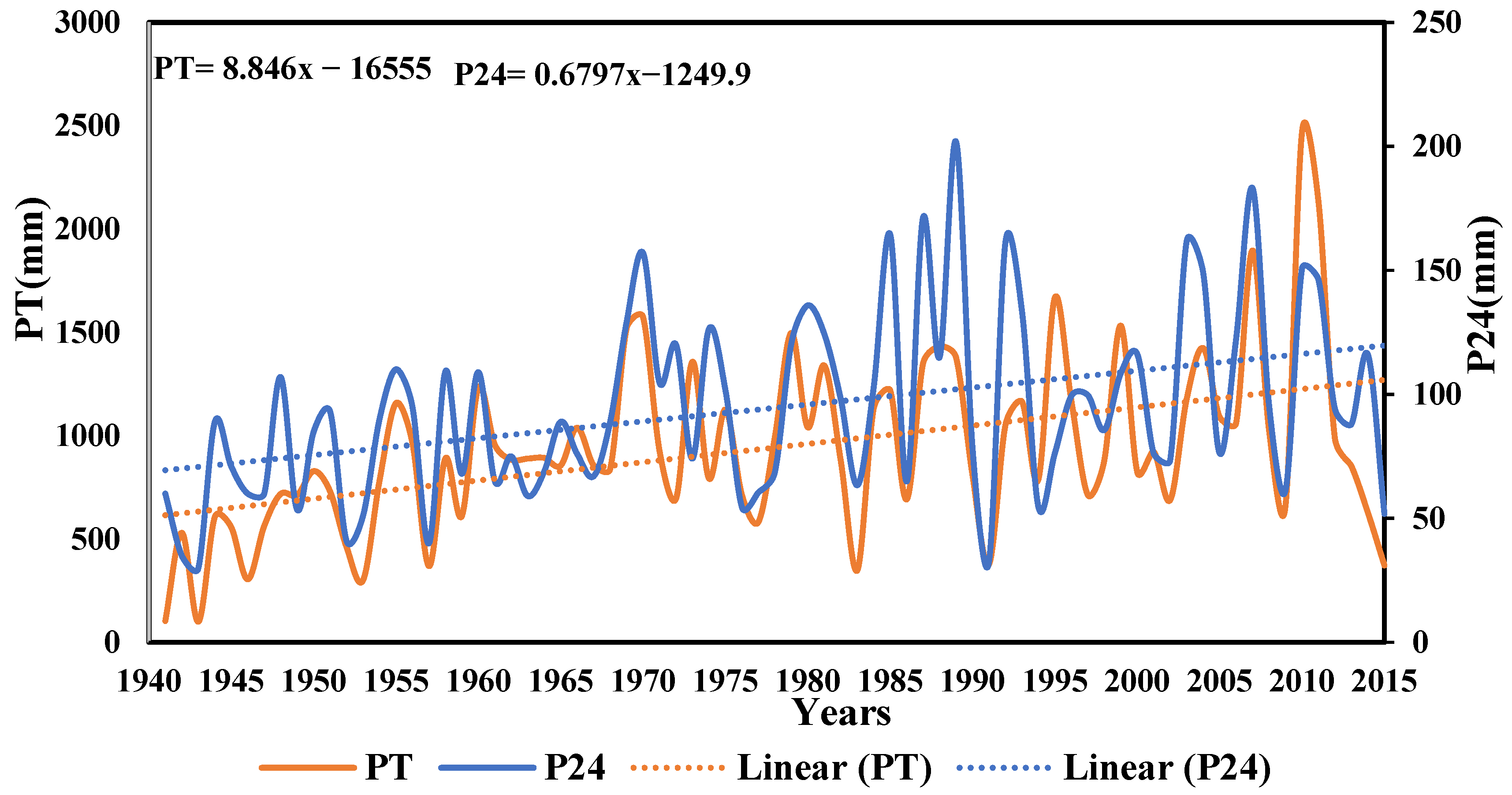
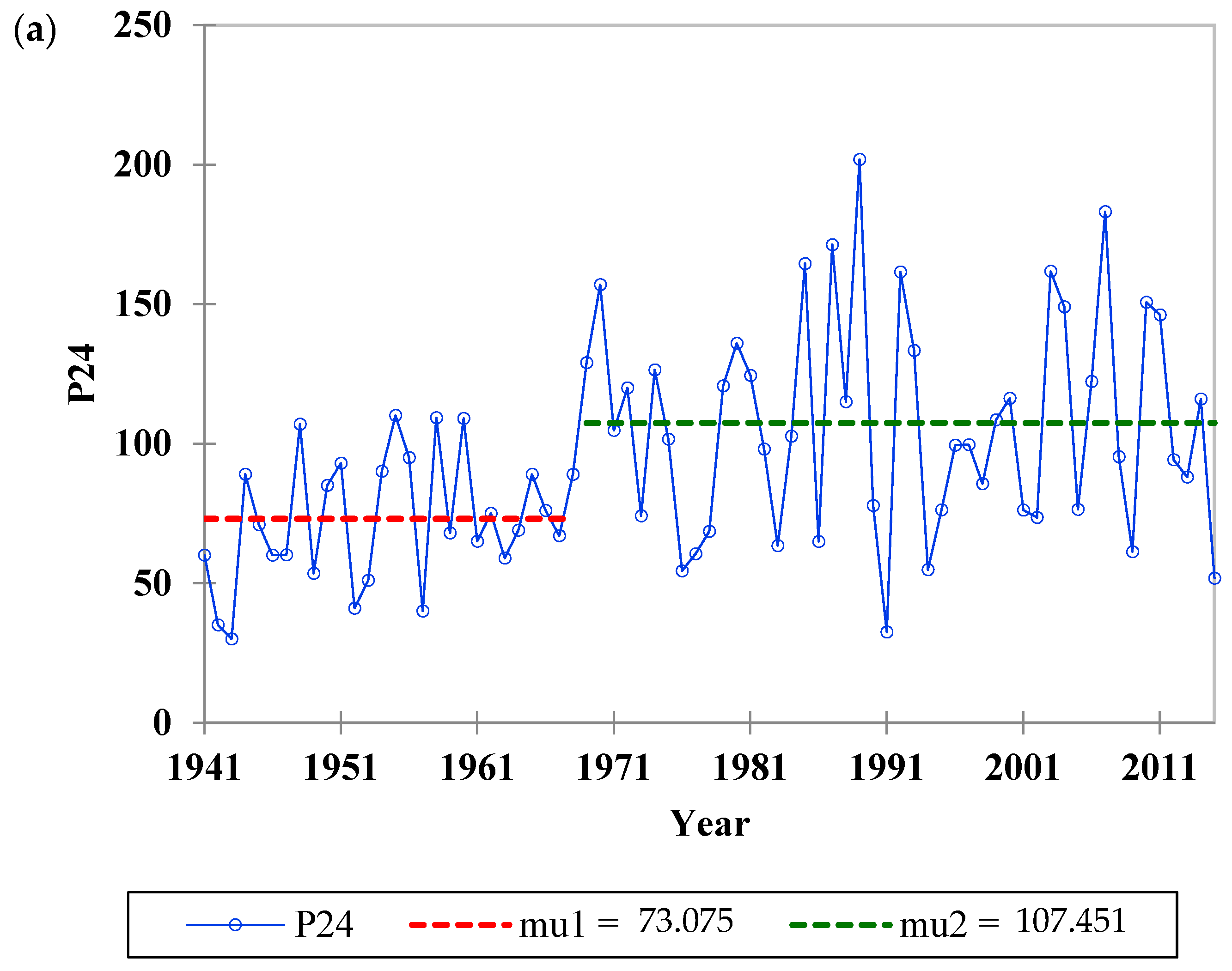
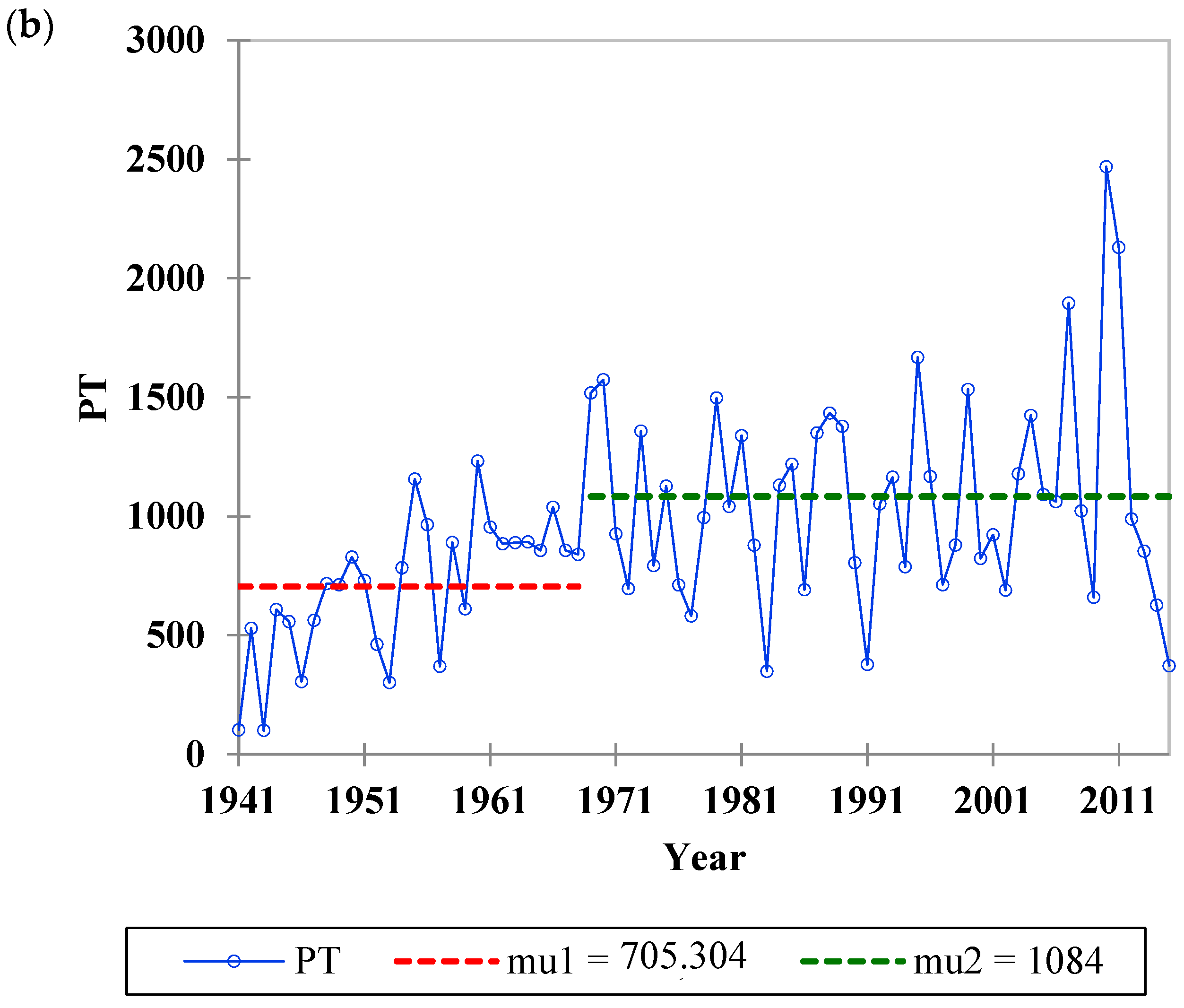
The results of the Buishand homogeneity test for P24 and PT are shown in Figure 4. The mean P24 in the period between 1941 and 1968 was 73.075 mm, and for the period from 1969 to 2015, it was 107.451 mm. For the PT, in the period from 1941 to 1968, the mean value was 705.304 mm (μ1), and between 1969 and 2015, the mean value was 1084 mm (μ2).
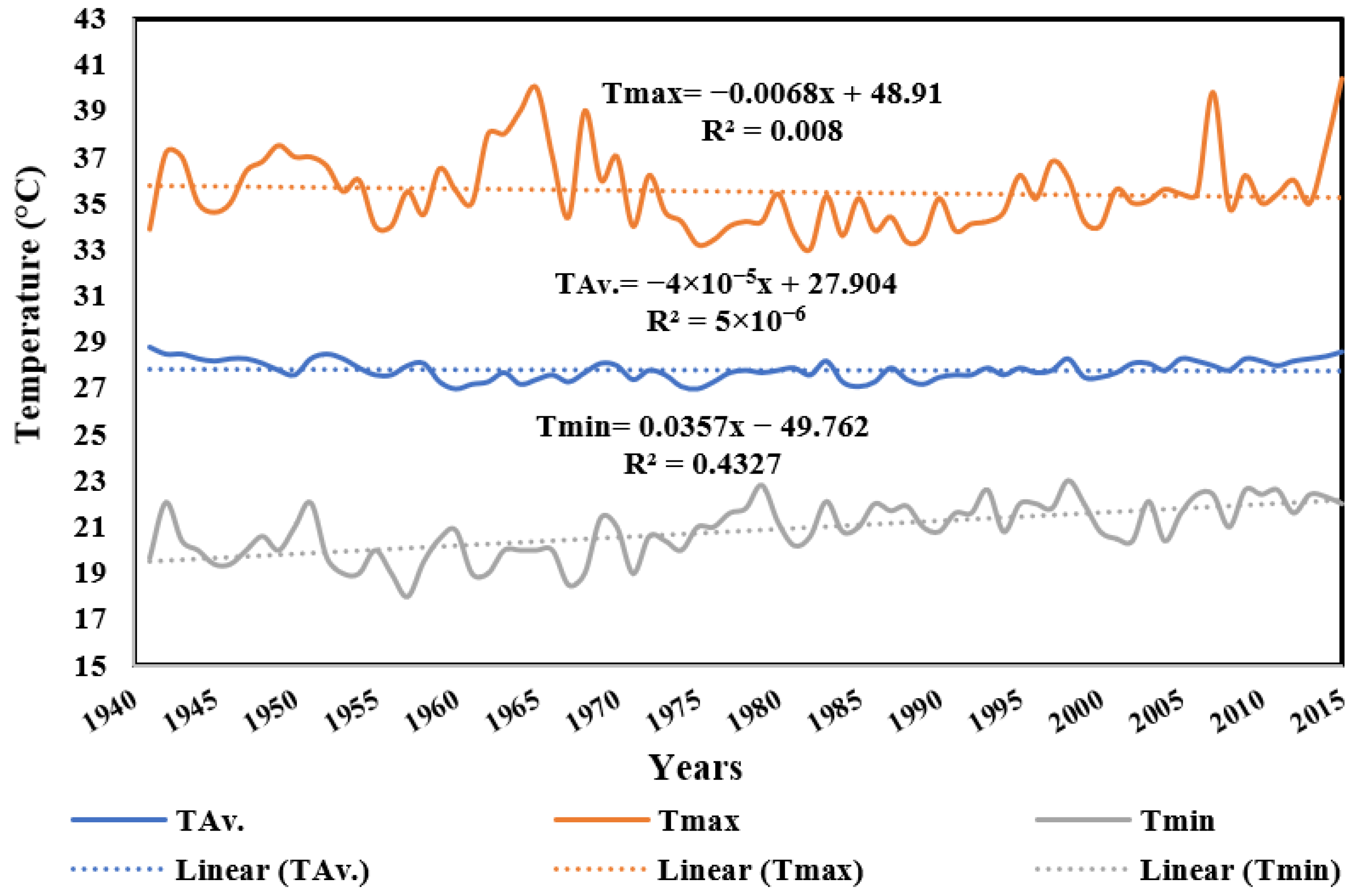
The results of the Buishand homogeneity test are shown for Tmax and Tmean. The mean value of Tmax between 1941 and 1970 was 36.296 °C, and between 1971 and 2015, it was 35.016 °C. For the Tmean, in the period between 1941 and 1958, it showed a mean value of 28.150 °C (μ1), and for the period from 1959 to 2015, the mean value was 27.716 °C (μ2).
The results of the Buishand homogeneity test are shown for the minimum temperature (Tmin). The mean value of Tmin between 1941 and 1974 was 19.882 °C (μ1), and between 1975 and 2015, the mean value was 21.620 °C (μ2).
These results show the non-homogeneity of the series, in which the total annual rainfall (PT) and the maximum rainfall in 24 h (P24) increased significantly (mean value) around the year 1968. The maximum temperature shows a sharp decline around the year 1970. Similarly, the average temperature shows a sharp decrease around 1958. However, the minimum temperature shows a sharp increase around the year 1974. These non-homogeneities are associated with changes in the location of the station or in instrumentation, among other aspects [32].

4.2. Tests of Stationarity and Trend

Using XLSTAT software, three tests of stationarity were performed (the Dickey–Fuller test, the Phillips–Perron test and the KPSS test) on the PT, P24, Tmax, Tmean and Tmin series. The results are shown in Table 3. According to the test results for the PT series, for two criteria (Dickey–Fuller and KPSS), the series was stationary, but for the Phillips–Perron criterion, the series was non-stationary. For the P24 series, two criteria showed results of non-stationarity (Dickey–Fuller and Phillips–Perron), and one showed stationarity (KPSS). For the maximum and mean temperature series, all the criteria showed non-stationarity results. For the minimum temperature series, two criteria showed non-stationarity (Dickey–Fuller and Phillips–Perron), and the KPSS criterion showed that the series was stationary.
According to the Mann–Kendall criterion, the series of total precipitation (PT), maximum precipitation in 24 h (P24) and minimum temperature (Tmin) showed trends, whereas the series of maximum temperature (Tmax) and average temperature (Tmean) showed no trend.
According to the results of the stationarity test obtained with the Phillips–Perron criterion, all series were non-stationary. For the two additional stationarity tests, 40% were shown to be stationary and 60% were non-stationary. For the Mann–Kendall trend test, 60% had a trending series, and 40% were trendless.
It is interesting to compare some case studies in the literature with the present results. Viloria-Marimón et al. (2019) evaluated the trend of 19 registered series of maximum rainfall in 24 h from the department of Atlántico, Colombia. They found that 10 series showed increasing trends, and eight series showed decreasing trends. Additionally, they estimated the maximum rainfall in 24 h, applying the criteria of stationarity and non-stationarity regardless of whether the series were stationary or not. In a similar way, Tekleab et al. (2013) analyzed the hydroclimatic trends in the upper part of the Blue Nile basin in Ethiopia. They found heterogeneous results, where the mean temperature had increased (0.3 °C in the rainy season and 0.6 °C in the dry season) but the time series of precipitation did not show statistically significant trends. Finally, Gonzalez-Alvarez et al. (2018), analyzing the 24 h precipitation series at the Rafael Núñez Airport station of Cartagena (the same series analyzed in this work), identified a trend over time. Therefore, they proposed the use of the frequency criterion for evaluating non-stationary and stationary conditions, showing that the non-stationary condition better represented the series. The estimates of the maximum precipitation in 24 h were higher (6–44%) than the estimates with stationarity. However, the series presented homogeneity problems (Figure 3), which generated the apparent trend.

4.3. Correction for Non-Homogeneity

Considering that all the analyzed series presented homogeneity problems, they were adjusted to coincide with the final section of the series. The series of adjusted temperatures were labeled as Tmax-R, -R, Tmin-R, P24-C and PT-C. To correct the series for non-homogeneity, the following equation was used (1):
x t = x t X 1 S 1 ( X ) S 2 ( X ) + X 2
where X t is the value adjusted for non-homogeneity, x t is the initial value of the subseries used to adjust for non-homogeneity, X 1 is the mean value of subseries 1, X 2 is the mean value of subseries 2, S 1 ( X ) is the standard deviation of subseries 1 and S 2 ( X ) is the standard deviation of subseries 2.
Table 4 shows how the temporal correlation of the minimum temperature decreases to almost zero after correction for homogeneity. The correlations of the maximum rainfall in 24 h and the total rainfall with the minimum temperature, after correcting for non-homogeneity, decreased by more than 100%. A higher temporal correlation value appears for the maximum (0.26) and mean (0.35) temperatures after correcting for non-homogeneity. For the correlation of the maximum rainfall in 24 h and the total annual rainfall with the mean temperature, the two analyses showed similar results. The correlation of the maximum precipitation in 24 h and the total annual precipitation with the maximum temperature tended to zero after adjusting the series for non-homogeneity.
Non-homogeneity alters the statistical parameters of the series and the cross-correlations between them, which can lead to biased interpretations.
In analyses of the series of total annual precipitation and maximum precipitation in 24 h, as well as maximum, average and minimum temperatures, at the Rafael Núñez Airport station in the city of Cartagena from 1941 to 2015, it can be seen that there is a significant correlation between maximum rainfall in 24 h and total annual precipitation (0.66).
Additionally, all the series presented non-homogeneity problems. The non-homogeneity of the minimum temperature series suggests a significant temporal correlation (0.66) and an intermediate correlation (0.33, 0.38) with the maximum precipitation in 24 h and with the total annual precipitation. These correlations tended to low values when non-homogeneity correction was applied.
The mean temperature showed an intermediate temporal correlation (0.35) and negative correlations with the maximum precipitation in 24 h (−0.24) and with the total annual precipitation (−0.28). Ultimately, non-homogeneity tests are one of the most important tests in climate studies. To obtain reliable results, meteorological data must be homogeneous [32].

4.4. Periodicity Analysis

To identify the periodic components of the series corrected for homogeneity, we subjected them to spectral analysis using XLSTAT software.
In Table 5, the results for each series of the periodograms are shown. The most important values for determining the periodic frequencies are highlighted in different colors. The highest values are shown in red, the second highest values in yellow and the third highest values in green. The values shaded in blue represent doubtful values, whereas those in gray are the missing data, the values shaded in blue represent doubtful values, finally, the series in light green were filled with random data that met the mean and variance.
The results show predominant periodicities in the series for periods of 75 and 37.5 years, around 15 and 18.75 years, around 10 years, around 5 years and around 3.75 years. The weighted sum column refers to the sum of the values of the maximum precipitation in 24 h plus the values corresponding to the total precipitation plus the values corresponding to the average of the values recorded for average, maximum and minimum temperatures. According to this criterion, the frequency of greatest significance is 3.75 years, followed by 37.5 years and, in descending order, 75, 4.69 and 6.25 years.
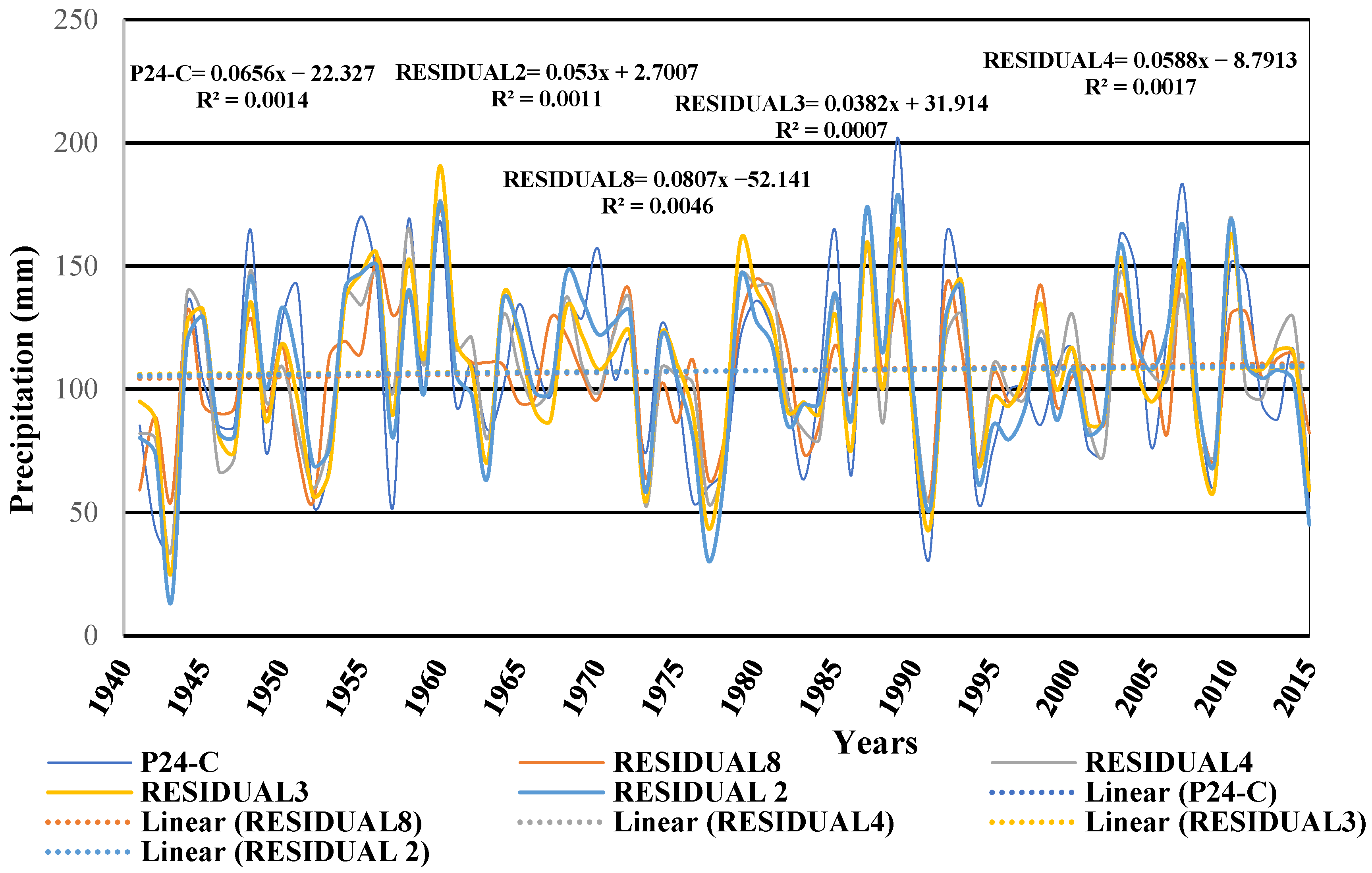
The eight frequencies with the highest intensities were selected for analysis. For each of the selected frequencies, its harmonic components were calculated, and the periodic functions of each frequency were generated. A residual function consisting of the original function minus the periodic functions selected from the spectral analysis was generated. For example, the Residual 8 function was obtained as the original series minus the eight periodic series generated with the eight highest-valued frequencies. Similarly, Residual Series 4 was the result of subtracting the four most important periodic series obtained from the spectral analysis from the original series. Residual series were generated and named Residual 8, Residual 4, Residual 3 and Residual 2 for each of the variables.
For the specific case of the series of maximum rainfall in 24 h (P24-C), the order of importance of the frequencies existing in the series according to the spectral analysis, from highest to lowest, is 3.75 years, 15.22 and 2.42 years, 7.68 and 18.75 years, 7.42 and 4.69 years, 6.57 and 3.41 years, 5.84 and 5 years, 4.13 and 2.08 years, 4.71 and 3.26 years, and 3.7 years. Therefore, the Residual 8 series is equal to the series of maximum precipitation in 24 h (P24-C) minus the eight periodic series with frequencies of 3.75, 2.42, 18.75, 4.69, 3.41, 5, 2.08 and 3.26 years. The Residual 4 series corresponds to the series of maximum precipitation in 24 h (P24-C) minus the four periodic series with frequencies of 3.75, 2.42, 18.75 and 4.69 years, and so on for the Residual 3 and Residual 2 series.
The frequencies that showed the strongest signals in the spectral analysis for all the series were 75, 37.5, 18.75, 15.6. 25, 5, 4.69, 3.75, 3.41, 2.88 and 2.42 years.
By considering the weighted sum of the signal of each series, we found that the periodic frequencies of greatest significance, in descending order, were 3.75 years, followed by 37.5, 75, 4.69 and 6.25 years (the five largest). All the series analyzed from the second harmonic showed no trend.
A significant presence of frequencies of 3.75 and 4.69 years was found, which could be considered to be part of the anomalies of the Pacific and tropical Atlantic. In the maximum rainfall in 24 h, the frequency of 2.42 years appears, which could be associated with the quasi-biennial oscillation of the zonal wind in the lower stratosphere, whereas the frequency of 18.75 is associated with the Pacific decadal oscillation. The 4–5-year signal associated with the tropical Pacific and Atlantic anomalies is marked in the minimum temperature series with frequencies of 3.95, 4.41 and 4.69 years. The frequency of 37.5 years is marked in the series for total annual precipitation, as well as maximum and mean temperature.
In studies of the time series of aquifers [33] using piezometers, for example, cyclicities (11–22 years) related to solar cycles of 11 and 3.2 years associated with the North Atlantic oscillation (NAO) were found.
Rodríguez and Llasat (1997) [34] analyzed the monthly precipitation series of Barcelona (Spain) between 1850 and 1991. They found a trend of increasing precipitation. A semi-annual periodicity (0.5 years) and two periodicities between 6.0 and 7.2 years and 19 to 24 years with little amplitude and no real meaning were found.
Figure 5 shows the curves of maximum precipitation in 24 h and Residuals 8, 4, 3 and 2 with their respective trend lines. The smallest slope of the residual series is represented by Residual 3.
For the series of total annual precipitation, the frequencies with the greatest intensity are, in decreasing order, 37.5, 3.75, 6.25, 2.88, 5, 25, 3.13 and 15 years. The Residual 8 series for total annual precipitation is the total annual precipitation series (PT-C) minus the eight periodic series with frequencies of 37.5, 3.75, 6.25, 2.88, 5, 25, 3.13 and 15 years. The other residual series are constructed in a similar way.
Similar analyses were carried out for the other series. The results for the total annual precipitation and Residuals 8, 4, 3 and 2 are shown, with their respective trend lines and the linear function calculated for each series. The smallest slope of the residual series is represented by Residual 2, followed by Residual 3.
For the mean temperature, the predominant frequencies, in order of importance, are 75, 37.5, 5, 12.5, 5.77, 3.57, 15 and 6.25 years. The slopes of the lines of the residual series are lower than the slope of the original series.
For maximum temperature, the frequencies of the greatest significance, in descending order, are 37.5, 15, 75, 10.71, 2.78, 2.5, 3.57 and 25 years. The decrease in the slopes of the residual series is appreciable compared with the original series.
For the minimum temperature, the frequencies of the greatest significance determined by spectral analysis are 4.69, 9.38, 3.41, 3.95, 6.82, 75, 4.41 and 2.03 years. The slopes of the original function and the residual functions remained at values of a similar magnitude. The minimum temperatures showed different frequency signals from the other series in general terms.
In summary (Table 5), the total annual precipitation, the maximum temperature and the average temperature showed a significant frequency of 37.5 years. Maximum rainfall in 24 h and minimum temperature showed significant frequency signals of 4.69 and 3.41 years, respectively.
The slope of the trend line showed a general trend of a decrease compared with the number of harmonics considered (Table 6). Only the maximum precipitation in 24 h showed different behavior. Up to the third harmonic, all slopes decreased.

4.5. Effect of Periodicity on Stationarity and Trends

Here, we describe the results of the stationarity and trend tests applied to all the initial series (PT, P24, Tmax, Tmean and Tmin), those adjusted for non-homogeneity (PT-C, P24-C, Tmax-R, Tmean-R and Tmin-R) and their corresponding residuals (Residual 2 (R2), Residual 3 (R3), Residual 4 (R4) and Residual 8 (R8)).
In Appendix B, the results of the stationarity and trend tests are shown for total precipitation (PT); adjusted total precipitation (PT-C); and the corresponding residual functions with two harmonics (PTC-R2), three harmonics (PTC-R3), four harmonics (PTC-R4) and eight harmonics (PTC-R8). Likewise, stationarity and trend tests were carried out for the other series under study (P24, P24-C, P24-C-R2, P24-C-R3, P24-C-R4 and P24-C-R8 for total rainfall in 24 h and all temperature series (maximum, mean and minimum)), as shown in Appendix B. According to the results of the Phillips–Perron test, all the series are non-stationary. Therefore, this test was not sensitive in the case of our study and was considered in the analysis of the results.
According to the Dickey–Fuller test, the original series of total precipitation was stationary after adjustment for non-homogeneity. When the periodicities (two, three, four and eight harmonics) were extracted, stationary series were revealed. According to the KPSS test, all total precipitation series were stationary. The Mann–Kendall trend tests showed that the original series of total precipitation had a trend, but after adjustment for non-homogeneity, no trend was recorded for any of the residual series.
The original series of maximum precipitation in 24 h was non-stationary according to the Dickey–Fuller test. On the other hand, when it was adjusted for non-homogeneity, the result was stationary, and when the periodicities (two, three, four and eight harmonics) were extracted, the result showed a stationary series. According to the KPSS test, all 24 h precipitation series were stationary. The Mann–Kendall trend test showed that the original 24-h precipitation series had a trend, but after it was adjusted for non-homogeneity, no trend was recorded in any of the residual series.
Moreover, according to the Dickey–Fuller test for the original maximum temperature series adjusted for non-homogeneity and after two harmonics (Residual 2) had been extracted, a non-stationary series was found. The series corresponding to Residuals 3, 4 and 8 are stationary. The KPSS test gave non-stationary results both for the original maximum temperature series and the series adjusted for non-homogeneity. The series of Residuals 2, 3, 4 and 8 gave stationary results. The Mann–Kendall trend tests showed that for all series, no trends were recorded.
The results of the Dickey–Fuller test showed a non-stationary series both for the original mean temperature series, as well as the series adjusted for non-homogeneity. The series corresponding to Residuals 2, 3, 4 and 8 provided stationary results. According to the KPSS test, the original mean temperature series and the series adjusted for non-homogeneity showed non-stationarity results. The series of Residuals 2, 3, 4 and 8 showed stationary results. The Mann–Kendall trend tests showed that in the series of mean temperature adjusted for non-homogeneity, there was a trend, whereas in the other series, no trend was found.
Finally, according to the Dickey–Fuller test for the minimum temperature series adjusted for non-homogeneity, the result was a stationary series. The other series gave non-stationary results. According to the KPSS test, all the minimum temperature series gave results of stationarity. The series of Residuals 2, 3, 4 and 8 gave stationary results. The Mann–Kendall trend tests showed a trend in the original minimum temperature series, whereas in the other cases, no trend was shown.
In summary, all the series were insensitive to the Phillips–Perron criterion because all the series in any condition were non-stationary. Here, 60% of the original series (PT, P24, Tmax, Tmean and Tmin) were shown to be non-stationary, and 40% were stationary. In 60% of the cases, a trend was shown. When the series were adjusted for non-homogeneity (PT-C, P24-C, Tmax-R, Tmean-R and Tmin-R), 50% remained non-stationary, and the other 50% were stationary. In this case, only 20% showed a trend, revealing the strong impact of non-homogeneity on the trend.
After extraction of the two harmonics of the greatest significance from the series, the percentage of non-stationary series was 20%, 80% were stationary and no series showed a trend. After extraction of the three, four and eight harmonics of greatest significance from the series, 10% of the series displayed non-stationarity, and 90% were stationary. None of the series showed a trend (Appendix C).
In earlier work, Viloria-Marimón et al. (2019) [35] studied the maximum precipitation data in 19 pluviographs in a region of Colombia. They evaluated the trends of the series and found positive and negative trends. Additionally, they applied the concepts of frequency for stationary and non-stationary series, estimating the values of maximum precipitation in 24 h for different return periods. However, the homogeneity of the series and the periodicity contained in the records, which could affect the reliability of the results, were not considered [32]. When these adjustments are not applied, apparent trends can be obtained. In the case of negative trends, this could lead to underestimations of the design parameters, leaving communities exposed and vulnerable to the original problem. In the opposite case, an overestimation of the design parameters could lead to negative economic consequences for the designs [36].

5. Discussion

For the stationarity test, we applied several criteria. The results obtained with the Phillips–Perron criterion were all non-stationary series; when the two additional criteria were applied, the results obtained were 40% stationary and 60% non-stationary; and when the Mann–Kendall criterion was applied, 60% were found to be trending series, and 40% were trendless.
It is interesting to compare some case studies in the literature with the present results. As previously mentioned, the work by Viloria-Marimón et al. (2019) [35] evaluated the trend of 19 registered series of maximum rainfall in 24 h in the department of Atlántico, Colombia. They found that 10 series showed increasing trends, whereas eight series showed decreasing trends. Additionally, they estimated the maximum rainfall in 24 h by applying criteria of stationarity and non-stationarity, regardless of whether the series were stationary or not. In a similar way, Tekleab et al. (2013) [19] analyzed the hydroclimatic trends in the upper part of the Blue Nile basin in Ethiopia. They found heterogeneous results, where the mean temperature had increased (0.3 °C in the rainy season and 0.6 °C in the dry season) but the time series of precipitation did not show statistically significant trends. Finally, Gonzalez-Alvarez et al. (2018) [11] evaluated the 24 h precipitation series at the Rafael Núñez Airport station of Cartagena and identified a trend over time. Consequently, they proposed the use of the frequency criterion for non-stationary and stationary conditions, showing that the non-stationary condition better represents the series. Nevertheless, according to the results of this research, this is an apparent trend.
Therefore, non-homogeneity problems and apparent trends associated with climate change could have negative implications for the design of drainage systems. There is a growing tendency to claim that the theory of non-stationarity has died due to the effects of climate change. This has led to inadequate legislation in some countries, such as Colombia, forcing engineers to apply new and developing calculation hypotheses.
The main limitation of this study is the data, as they were obtained from a single station.

6. Conclusions

The objective of the present work was to analyze descriptive statistical parameters as basic elements for making decisions about the effects of climate change in an undeveloped area in Latin America and to realize a statistical analysis of a time series of the basic weather parameters in the city of Cartagena normally used to design drainage systems. Currently, the stationarity criterion is in force for calculating the hydrological design parameters of the Rafael Núnez Airport station in the city of Cartagena. In the case of this study, a non-homogeneity problem was highlighted, producing apparent trends possibly associated with climate change effects. Nevertheless, the studied series are non-stationary, and a new paradigm is most likely required for estimating the design parameters of engineering works.
The series are non-stationary due to the omission of homogeneity and a periodicity analysis of the original series. This could lead to misevaluated engineering design parameters, which could result in unpredictable negative consequences. Finally, the apparent trend shown by the original series is due to problems of non-homogeneity and the influence of periodicity (climate variability), whereby no evidence of climate change effects was found.

Author Contributions

Conceptualization, A.A.-P., M.S. and A.P.A.; methodology, A.A.-P., M.S. and A.P.A.; software, A.A.-P.; validation, A.A.-P.; formal analysis, A.A.-P.; investigation, A.A.-P., M.S. and A.P.A.; resources, A.A.-P., M.S. and A.P.A.; data curation, M.S.; writing—original draft preparation, A.A.-P. and M.S.; writing—review and editing, M.S.; visualization, M.S.; supervision, M.S.; project administration, M.S.; funding acquisition, A.A.-P. All authors have read and agreed to the published version of the manuscript.

Funding

This research received no external funding.

Institutional Review Board Statement

Not applicable.

Informed Consent Statement

Not applicable.

Data Availability Statement

Data are available upon reasonable request.

Acknowledgments

The authors would like to acknowledge the IDEAM for providing the data on which this study was based.

Conflicts of Interest

The authors declare no conflict of interest.

Appendix A

Table A1. Complete data of the series.
Information Taken from IDEAMInformation Taken from IDEAM (Filling in Missing Data)
YearsP24PTTmeanTmaxTminYearsP24PTTmeanTmaxTmin
194160103.428.8 194160103.428.833.8719.67
194235530.228.5 194235530.228.537.1822.05
194330100.928.53720.4194330100.928.53720.4
194489608.228.33520194489608.228.33520
194571557.628.234.619.4194571557.628.234.619.4
194660305.228.33519.4194660305.228.33519.4
194760.1564.128.336.420194760.1564.128.336.420
1948107717.828.136.820.61948107717.828.136.820.6
194953.5712.727.837.520194953.5712.727.837.520
195085829.127.63721195085829.127.63721
195193730.328.337 195193730.328.33722.05
195241462.328.536.6 195241462.328.536.619.67
195351301.228.335.519195351301.228.335.519
195490.1784.427.93619195490.1784.427.93619
1955110.11157.327.634201955110.11157.327.63420
195695964.727.63419195695964.727.63419
195740369.92835.518195740369.92835.518
1958109.3890.628.134.519.51958109.3890.628.134.519.5
195968611.627.336.520.5195968611.627.336.520.5
19601091232.227 19601091232.22735.5320.86
196165955.627.23519196165955.627.23519
196275884.827.33819196275884.827.33819
196359889.227.73820196359889.227.73820
196469892.427.23920196469892.427.23920
196589856.827.44020196589856.827.44020
1966761039.127.637201966761039.127.63720
196767856.927.334.418.5196767856.927.334.418.5
19688984027.7391919688984027.73919
19691291518.128.13621.419691291518.128.13621.4
19701571574.428372119701571574.4283721
1971104.7926.427.434191971104.7926.427.43419
1972120697.127.836.220.61972120697.127.836.220.6
197374.11358.327.634.620.4197374.11358.327.634.620.4
1974126.4793.827.134.2201974126.4793.827.134.220
1975101.61126.82733.2211975101.61126.82733.221
197654.4711.727.333.421197654.4711.727.333.421
197760.5582.227.73421.6197760.5582.227.73421.6
197868.6994.627.834.221.8197868.6994.627.834.221.8
1979120.71497.527.734.222.81979120.71497.527.734.222.8
1980135.91041.427.835.421.21980135.91041.427.835.421.2
1981124.41340.127.933.720.21981124.41340.127.933.720.2
198298878.327.63320.6198298878.327.63320.6
198363.4349.128.235.322.1198363.4349.128.235.322.1
1984102.71130.927.333.620.81984102.71130.927.333.620.8
1985164.51219.227.135.2211985164.51219.227.135.221
198664.9692.527.333.822198664.9692.527.333.822
1987171.31350.827.934.421.71987171.31350.827.934.421.7
19881151433.727.433.321.919881151433.727.433.321.9
1989201.8137827.233.5211989201.8137827.233.521
199077.8805.627.535.220.8199077.8805.627.535.220.8
199132.5378.327.633.821.6199132.5378.327.633.821.6
1992161.5105327.634.121.61992161.5105327.634.121.6
1993133.41165.227.934.222.61993133.41165.227.934.222.6
199454.8788.527.634.620.8199454.8788.527.634.620.8
199576.31668.627.936.222199576.31668.627.936.222
199699.4116827.735.222199699.4116827.735.222
199799.6712.727.836.821.8199799.6712.727.836.821.8
199885.6880.228.336.123199885.6880.228.336.123
1999108.51532.927.534.2221999108.51532.927.534.222
2000116.2823.327.53420.82000116.2823.327.53420.8
200176.2922.827.735.620.5200176.2922.827.735.620.5
200273.5689.628.13520.4200273.5689.628.13520.4
2003161.81178.928.135.122.12003161.81178.928.135.122.1
20041491423.927.835.620.420041491423.927.835.620.4
200576.41091.328.335.421.6200576.41091.328.335.421.6
2006122.31061.728.235.422.42006122.31061.728.235.422.4
2007183.11895.92839.822.42007183.11895.92839.822.4
200895.31022.727.834.821200895.31022.727.834.821
200961.3660.728.336.222.6200961.3660.728.336.222.6
2010150.72469.228.23522.42010150.72469.228.23522.4
2011146.12130.22835.422.62011146.12130.22835.422.6
201294.2988.528.23621.6201294.2988.528.23621.6
201388853.728.33522.4201388853.728.33522.4
2014116627.228.437.422.32014116627.228.437.422.3
201551.8372.328.640.422201551.8372.328.640.422

Appendix B

Table A2. Results of the stationarity and trend tests for total precipitation (PT-C) and the residual functions with two harmonics (PTC-R2), three harmonics (PTC-R3), four harmonics (PTC-R4) and eight harmonics (PTC-R8).
StationarityTrend
Description of the VariableVariableDickey–FullerPhillips–PerronKPSSMann–Kendall
Total precipitationPTStationaryNot stationaryStationaryTrend
Total precipitation adjusted for homogeneityPT-CNot stationaryNot stationaryStationaryNo trend
Total precipitation adjusted for homogeneity, Residual 2PT-C-R2StationaryNot stationaryStationaryNo trend
Total precipitation adjusted for homogeneity, Residual 3PT-C-R3StationaryNot stationaryStationaryNo trend
Total precipitation adjusted for homogeneity, Residual 4PT-C-R4StationaryNot stationaryStationaryNo trend
Total Precipitation adjusted for homogeneity, Residual 8PT-C-R8StationaryNot stationaryStationaryNo trend
Maximum rainfall in 24 hP24Not stationaryNot stationaryStationaryTrend
Maximum rainfall in 24 h adjusted for homogeneityP24-CStationaryNot stationaryStationaryNo trend
Maximum precipitation in 24 h (P24) adjusted for homogeneity, Residual 2P24-C-R2StationaryNot stationaryStationaryNo trend
Maximum precipitation in24 h (P24) adjusted for homogeneity, Residual 3P24-C-R3StationaryNot stationaryStationaryNo trend
Maximum precipitation in 24 h (P24) adjusted for homogeneity, Residual 4P24-C-R4StationaryNot stationaryStationaryNo trend
Maximum precipitation in 24 h (P24) adjusted for homogeneity, Residual 8P24-C-R8StationaryNot stationaryStationaryNo trend
Annual maximum temperatureTmaxNot stationaryNot stationaryNot stationaryNo trend
Annual maximum temperature adjusted for homogeneityTmax-RNot stationaryNot stationaryNot stationaryNo trend
Annual maximum temperature adjusted for homogeneity, Residual 2Tmax-R-R2Not stationaryNot stationaryStationaryNo trend
Annual maximum temperature adjusted for homogeneity, Residual 3Tmax-R-R3StationaryNot stationaryStationaryNo trend
Annual maximum temperature adjusted for homogeneity, Residual 4Tmax-R-R4StationaryNot stationaryStationaryNo trend
Annual maximum temperature adjusted for homogeneity, Residual 8Tmax-R-R8StationaryNot stationaryStationaryNo trend
Annual mean temperatureTmeanNot stationaryNot stationaryNot stationaryNo trend
Annual mean temperature adjusted for homogeneityTmean-RNot stationaryNot stationaryNot stationaryTrend
Annual mean temperature adjusted for homogeneity, Residual 2Tmean-R-R2StationaryNot stationaryStationaryNo trend
Annual mean temperature adjusted for homogeneity, Residual 3Tmean-R-R3StationaryNot stationaryStationaryNo trend
Annual mean temperature adjusted for homogeneity, Residual 4Tmean-R-R4StationaryNot stationaryStationaryNo trend
Annual mean temperature adjusted for homogeneity, Residual 8Tmean-R-R8StationaryNot stationaryStationaryNo trend
Annual minimum temperatureTminNot stationaryNot stationaryStationaryTrend
Annual minimum temperature adjusted for homogeneityTmin-RStationaryNot stationaryStationaryNo trend
Annual minimum temperature adjusted for homogeneity, Residual 2Tmin-R-R2Not stationaryNot stationaryStationaryNo trend
Annual minimum temperature adjusted for homogeneity, Residual 3Tmin-R-R3Not stationaryNot stationaryStationaryNo trend
Annual minimum temperature adjusted for homogeneity, Residual 4Tmin-R-R4Not stationaryNot stationaryStationaryNo trend
Annual minimum temperature adjusted for homogeneity, Residual 8Tmin-R-R8Not stationaryNot stationaryStationaryNo trend

Appendix C

Table A3. Series Adjusted for Non-Homogeneity.
Series Adjusted for Non-Homogeneity
YearsP24-CPT-CTmean-RTmax-RTmin-R
194185.3171.628.532.721.4
194243.0818.828.135.923.3
194334.5167.828.135.722.0
1944134.4937.027.933.821.7
1945103.9860.327.833.421.2
194685.3477.627.933.821.2
194785.5870.227.935.121.7
1948164.91103.227.735.522.1
194974.31095.527.336.221.7
1950127.61272.027.135.722.5
1951141.21122.227.935.723.3
195253.1715.828.135.321.4
195370.1471.527.934.320.9
1954136.31204.227.434.720.9
1955170.11769.627.132.821.7
1956144.61477.627.132.820.9
195751.5575.727.534.320.1
1958168.81365.227.733.321.3
195998.9942.227.335.222.1
1960168.31883.127.034.322.4
196193.81463.827.233.820.9
1962110.71356.427.336.620.9
196383.61363.127.736.621.7
1964100.61367.927.237.621.7
1965134.41314.027.438.521.7
1966112.41590.427.635.721.7
196797.21314.127.333.220.5
1968134.41288.527.737.620.9
1969129.01518.128.134.722.8
1970157.01574.428.035.722.5
1971104.7926.427.434.020.9
1972120.0697.127.836.222.1
197374.11358.327.634.622.0
1974126.4793.827.134.221.7
1975101.61126.827.033.221.0
197654.4711.727.333.421.0
197760.5582.227.734.021.6
197868.6994.627.834.221.8
1979120.71497.527.734.222.8
1980135.91041.427.835.421.2
1981124.41340.127.933.720.2
198298.0878.327.633.020.6
198363.4349.128.235.322.1
1984102.71130.927.333.620.8
1985164.51219.227.135.221.0
198664.9692.527.333.822.0
1987171.31350.827.934.421.7
1988115.01433.727.433.321.9
1989201.81378.027.233.521.0
199077.8805.627.535.220.8
199132.5378.327.633.821.6
1992161.51053.027.634.121.6
1993133.41165.227.934.222.6
199454.8788.527.634.620.8
199576.31668.627.936.222.0
199699.41168.027.735.222.0
199799.6712.727.836.821.8
199885.6880.228.336.123.0
1999108.51532.927.534.222.0
2000116.2823.327.534.020.8
200176.2922.827.735.620.5
200273.5689.628.135.020.4
2003161.81178.928.135.122.1
2004149.01423.927.835.620.4
200576.41091.328.335.421.6
2006122.31061.728.235.422.4
2007183.11895.928.039.822.4
200895.31022.727.834.821.0
200961.3660.728.336.222.6
2010150.72469.228.235.022.4
2011146.12130.228.035.422.6
201294.2988.528.236.021.6
201388.0853.728.335.022.4
2014116.0627.228.437.422.3
201551.8372.328.640.422.0

References

  1. IPCC. Climate Change 2022: Impacts, Adaptation and Vulnerability|Climate Change 2022: Impacts, Adaptation and Vulnerability. 2022. Available online: https://www.ipcc.ch/report/ar6/wg2/ (accessed on 14 March 2022).
  2. Milly, P.C.D.; Betancourt, J.; Falkenmark, M.; Hirsch, R.M.; Kundzewicz, Z.W.; Lettenmaier, D.P.; Stouffer, R.J. Climate change: Stationarity is dead: Whither water management? Science 2008, 319, 573–574. [Google Scholar] [CrossRef]
  3. Kiang, J.E.; Olsen, J.R.; Waskom, R.M. Workshop on Nonstationarity, Hydrologic Frequency Analysis, and Water Management. Color. Water Inst. Inf. Ser. 2010, 1, 4–299. [Google Scholar]
  4. Matalas, N.C. Comment on the announced death of stationarity. J. Water Resour. Plan. Manag. 2012, 138, 311–312. [Google Scholar] [CrossRef]
  5. Montanari, A.; Koutsoyiannis, D. Modeling and mitigating natural hazards: Stationarity is immortal! Water Resour. Res. 2014, 50, 9748–9756. [Google Scholar] [CrossRef]
  6. Milly, P.C.D.; Betancourt, J.; Falkenmark, M.; Hirsch, R.M.; Kundzewicz, Z.W.; Lettenmaier, D.P.; Stouffer, R.J.; Dettinger, M.D.; Krysanova, V. On Critiques of ‘stationarity is Dead: Whither Water Management’? Water Resour. Res. 2015, 51, 7785–7789. [Google Scholar] [CrossRef] [Green Version]
  7. Koutsoyiannis, D.; Montanari, A. Negligent killing of scientific concepts: The stationarity case|Meurtre par imprudence de concepts scientifiques: Le cas de la stationnarité. Hydrol. Sci. J. 2015, 60, 7–8. [Google Scholar] [CrossRef]
  8. Poveda, G.; Álvarez, D.M. El colapso de la hipótesis de estacionariedad por cambio y variabilidad climática: Implicaciones para el diseño hidrológico en ingeniería. Rev. Ing. 2012, 36, 65–76. [Google Scholar] [CrossRef]
  9. Obeysekera, J.; Salas, J.D. Quantifying the uncertainty of design floods under nonstationary conditions. J. Hydrol. Eng. 2014, 19, 1438–1446. [Google Scholar] [CrossRef]
  10. Obeysekera, J.; Salas, J.D. Frequency of recurrent extremes under nonstationarity. J. Hydrol. Eng. 2016, 21, 1–9. [Google Scholar] [CrossRef]
  11. Gonzalez-Alvarez, A.; Coronado-Hernández, O.E.; Fuertes-Miquel, V.S.; Ramos, H.M. Effect of the non-stationarity of rainfall events on the design of hydraulic structures for runoff management and its applications to a case study at Gordo Creek watershed in Cartagena de Indias, Colombia. Fluids 2018, 3, 27. [Google Scholar] [CrossRef] [Green Version]
  12. Sharma, S.; Mujumdar, P.P. On the relationship of daily rainfall extremes and local mean temperature. J. Hydrol. 2019, 572, 179–191. [Google Scholar] [CrossRef]
  13. Naveendrakumar, G.; Vithanage, M.; Kwon, H.-H.; Chandrasekara, S.; Iqbal, M.; Pathmarajah, S.; Fernando, K.; Obeysekera, J. South Asian perspective on temperature and rainfall extremes: A review. Atmos. Res. 2019, 225, 110–120. [Google Scholar] [CrossRef]
  14. Fadhel, S.; Rico-Ramirez, M.A.; Han, D. Sensitivity of peak flow to the change of rainfall temporal pattern due to warmer climate. J. Hydrol. 2018, 560, 546–559. [Google Scholar] [CrossRef] [Green Version]
  15. Dey, P.; Mujumdar, P.P. On the uniformity of rainfall distribution over India. J. Hydrol. 2019, 578, 124017. [Google Scholar] [CrossRef]
  16. Samaniego, J.L. Cambio climático y desarrollo en América Latina y el Caribe: Una reseña; Cepal, Giz: Santiago de Chile, Chile, 2009. [Google Scholar]
  17. Pérez, C.; Poveda, G.; Mesa, O.; Carvajal, L.F.; Ochoa, A. Evidencias de cambio climático en Colombia: Tendencias y cambios de fase y amplitud de los ciclos anual y semianual. Bull. L’institut Français D’études Andin. 1998, 27, 537–546. [Google Scholar]
  18. Rougé, C.; Ge, Y.; Cai, X. Detecting gradual and abrupt changes in hydrological records. Adv. Water Resour. 2013, 53, 33–44. [Google Scholar] [CrossRef] [Green Version]
  19. Tekleab, S.; Mohamed, Y.; Uhlenbrook, S. Hydro-climatic trends in the Abay/Upper Blue Nile basin, Ethiopia. Phys. Chem. Earth 2013, 61–62, 32–42. [Google Scholar] [CrossRef]
  20. Mahmoud, S.H.; Gan, T.Y. Urbanization and climate change implications in flood risk management: Developing an efficient decision support system for flood susceptibility mapping. Sci. Total Environ. 2018, 636, 152–167. [Google Scholar] [CrossRef]
  21. Taxak, A.K.; Murumkar, A.R.; Arya, D.S. Long term spatial and temporal rainfall trends and homogeneity analysis in Wainganga basin, Central India. Weather Clim. Extrem. 2014, 4, 50–61. [Google Scholar] [CrossRef] [Green Version]
  22. Buishand, T.A.; Brandsma, T. Comparison of circulation classification schemes for predicting temperature and precipitation in The Netherlands. Int. J. Climatol. 1997, 17, 875–889. [Google Scholar] [CrossRef]
  23. Färe, R.; Primont, D.; Weber, W.L. Technical change and the von Neumann coefficient of uniform expansion. Eur. J. Oper. Res. 2020, 280, 754–763. [Google Scholar] [CrossRef]
  24. Steland, A. Weighted Dickey-Fuller processes for detecting stationarity. J. Stat. Plan. Inference 2007, 137, 4011–4030. [Google Scholar] [CrossRef] [Green Version]
  25. Escobari, D.; Garcia, S.; Mellado, C. Identifying bubbles in Latin American equity markets: Phillips-Perron-based tests and linkages. Emerg. Mark. Rev. 2017, 33, 90–101. [Google Scholar] [CrossRef] [Green Version]
  26. Lee, D.; Schmidt, P. On the power of the KPSS test of stationarity against fractionally-integrated alternatives. J. Econom. 1996, 73, 285–302. [Google Scholar] [CrossRef]
  27. De Jong, R.M.; Amsler, C.; Schmidt, P. A robust version of the KPSS test based on indicators. J. Econom. 2007, 137, 311–333. [Google Scholar] [CrossRef]
  28. Hamed, K.H. Trend detection in hydrologic data: The Mann-Kendall trend test under the scaling hypothesis. J. Hydrol. 2008, 349, 350–363. [Google Scholar] [CrossRef]
  29. Sun, S.; Fang, C. Water use trend analysis: A non-parametric method for the environmental Kuznets curve detection. J. Clean. Prod. 2018, 172, 497–507. [Google Scholar] [CrossRef]
  30. Shahid, M.; Rahman, K.U. Identifying the Annual and Seasonal Trends of Hydrological and Climatic Variables in the Indus Basin Pakistan. Asia-Pac. J. Atmos. Sci. 2020, 57, 191–205. [Google Scholar] [CrossRef]
  31. Shahid, M.; Cong, Z.; Zhang, D. Understanding the impacts of climate change and human activities on streamflow: A case study of the Soan River basin, Pakistan. Theor. Appl. Climatol. 2017, 134, 205–219. [Google Scholar] [CrossRef]
  32. Yozgatligil, C.; Yazici, C. Comparison of homogeneity tests for temperature using a simulation study. Int. J. Climatol. 2016, 36, 62–81. [Google Scholar] [CrossRef]
  33. Espinar, J.A.L.; Igúzquiza, E.P.; Olmo, M.C. Análisis de Ciclicidades de Series Hidrogeológicas en el Estudio de los Procesos de Recarga. 2005, pp. 451–458. Available online: https://dialnet.unirioja.es/servlet/articulo?codigo=5182254 (accessed on 10 March 2022).
  34. Rodríguez, R.; Llasat, M.C. Análisis Temporal y Espectral de la Serie de Precipitación Mensual de Barcelona España. Ing. Agua. 1997, 4, 19–28. [Google Scholar] [CrossRef] [Green Version]
  35. Viloria-Marimón, O.M.; González-Álvarez, Á.; Mouthón-Bello, J.A. Analysis of the behavior of daily maximum rainfall within the department of Atlántico, Colombia. Water 2019, 11, 2453. [Google Scholar] [CrossRef] [Green Version]
  36. Castro, L.M.; Escobar, Y.C. Análisis de tendencia y homogeneidad de series climatológicas. Ing. Recur. Nat. Ambient. 2010, 9, 15–25. [Google Scholar]
Figure 1. Location of the study area.
Water 14 01378 g001
Figure 2. Representation of the IDEAM series for total precipitation in 24 h (P24) and for total annual precipitation (PT).
Water 14 01378 g002
Figure 3. Representation of the time series of the maximum, mean and minimum temperatures recorded at the Rafael Núñez Airport station.
Water 14 01378 g003
Figure 4. Results of the Buishand test for (a) P24 and (b) PT.
Water 14 01378 g004aWater 14 01378 g004b
Figure 5. Maximum precipitation in 24 h and Residuals 2, 3, 4 and 8.
Water 14 01378 g005
Table 1. Descriptive statistical parameters of the series under analysis.
P24 (mm)PT (mm)Tmean (°C)Tmax (°C)Tmin (°C)
Mean94.62942.7827.8235.5320.86
Standard deviation37.71429.060.421.651.18
Variation coefficient0.400.460.020.050.06
Temporal correlation0.390.450.00−0.090.66
P24 correlation-0.71−0.20−0.150.33
PT correlation--−0.27−0.110.38
Table 2. Results of the homogeneity tests.
PettittSNHTBuishandVon Neumann
P240.00160.00270.00030.0685
PT0.00040.00260.00070.0005
Tmax0.00360.02760.0052<0.0001
Tmean0.0120.0000.005<0.0001
Tmin<0.0001<0.0001<0.0001<0.0001
α > 0.05: data are homogeneous; α < 0.05: there is a day when there is a change in the data.
Table 3. Results of the stationarity and trend tests for the PT, P24, Tmax, Tmean and Tmin series.
StationarityTrend
VariableDickey–FullerPhillips–PerronKPSSMann–Kendall
Total Precipitation (PT)(mm)StationaryNot stationaryStationaryTrend
Maximum rainfall in 24 h (P24)(mm)Not stationaryNot stationaryStationaryTrend
Annual maximum temperature (Tmax)(°C)Not stationaryNot stationaryNot stationaryNo trend
Average annual temperature (Tmean)(°C)Not stationaryNot stationaryNot stationaryNo trend
Annual minimum temperature (Tmin)(°C)Not stationaryNot stationaryStationaryTrend
Table 4. Effects of non-homogeneity on the statistical parameters of the series. See Table 1 for the original series and Appendix A for the complete data.
Series Adjusted for Non-Homogeneity
P24-C (mm)PT-C (mm)Tmean-R (°C)Tmax-R (°C)Tmin-R (°C)
Mean107.451084.2527.7235.0221.62
Standard deviation38.78435.530.391.490.74
Variation coefficient0.360.400.010.040.03
Temporal correlation0.040.120.350.260.08
Correlation with P24-C 0.66−0.24−0.030.10
Correlation with PT-C −0.280.040.17
Table 5. Summary of the periodogram resulting from the spectral analysis, expressed as a percentage for each series analyzed (based on XLSTAT results).
Periodicity (Years)P24-C (%)PT-C (%)Tmax-R (%)Tmean-R (%)Tmin-R (%)Weighted Sum (%)
0.000.000.000.000.000.000.00
75.000.611.886.8033.105.0117.46
37.502.3012.6611.7315.243.1825.01
25.003.285.813.920.823.6211.87
18.757.423.781.770.252.5412.72
15. 000.225.288.464.723.3611.01
12.501.332.771.425.592.807.37
10.713.402.956.332.221.199.60
9.380.160.073.032.1510.495.46
8.332.573.493.641.760.137.90
7.500.392.561.480.051.003.79
6.820.410.660.490.255.773.25
6.253.367.932.212.812.0713.65
5.770.051.030.895.340.543.33
5.362.250.372.410.870.613.92
5.004.136.131.086.112.4213.46
4.696.573.420.780.7112.2914.59
4.412.170.210.101.314.164.24
4.170.470.243.241.110.802.43
3.951.982.000.910.826.596.75
3.7515.228.471.821.563.5225.99
3.572.742.184.574.960.688.33
3.415.841.341.510.217.0610.10
3.263.701.301.540.681.776.33
3.131.825.640.780.071.408.21
3.003.061.780.760.360.495.38
2.880.316.453.662.041.019.00
2.780.630.385.960.030.463.15
2.681.710.901.240.023.064.05
2.591.661.101.080.260.743.46
2.500.860.845.281.161.284.27
2.427.680.212.590.760.949.31
2.341.090.800.200.483.233.20
2.272.590.840.400.040.083.60
2.210.731.120.530.740.052.29
2.140.170.673.040.831.242.54
2.084.710.651.180.160.686.03
2.032.412.093.170.423.726.94
Table 6. Slope of the trend line of each series analyzed.
HarmonicsTmin-RTmax-RTmean-RPT-CP24-C
00.00260.01760.00622.38240.0656
20.00340.00580.00030.13080.053
30.00170.00840.00040.41910.0382
40.00210.00570.00090.56880.0588
80.00190.00440.0003−1.19960.0807
Publisher’s Note: MDPI stays neutral with regard to jurisdictional claims in published maps and institutional affiliations.

